2 Methodology used for numerical simulation

The simulation data analysed in this paper are produced with a combination of implicit large-eddy simulation (ILES) and direct numerical simulation (DNS), both using the Navier–Stokes equations subject to the Boussinesq approximation. First, an ILES of each wake is run for a very long time in a computational domain sufficiently deep and wide to allow for the radiation and near-field propagation of wake-radiated internal waves, and with fine enough resolution to capture most of the turbulent motions. Next, selected snapshots in time of the full wake velocity and density fields are interpolated onto a very high-resolution DNS grid and advanced in time until the small-scale motions are in quasi-equilibrium with respect to the large-scale motions.

Before giving details of the ILES and DNS, let us consider the efficacy of studying DNS snapshots initialized with ILES. Since the wakes discussed in this paper are at much higher Reynolds number than those measured in the laboratory, no direct validations of the current results are possible. However, the ILES methodology has been demonstrated to reproduce important characteristics of laboratory wakes at lower Reynolds number (Spedding Reference Spedding1997, Reference Spedding2002; Diamessis, Spedding & Domaradzki Reference Diamessis, Spedding and Domaradzki2011). Additionally, Lalescu, Meneveau & Eyink (Reference Lalescu, Meneveau and Eyink2013) find that turbulent motions at scales smaller than 20 times the Kolmogorov length scale, ${\it\eta}$ , are slaved to the chaotic motions of the larger scales. So, provided the ILES is sufficiently resolved, the smaller scales of the DNS fill in without changing the larger scales. By comparing the DNS and ILES results, it is observed that the ILES grid spacing is never more than $20{\it\eta}$ . We conclude, therefore, that the DNS can be expected to produce the correct dynamics of the wakes considered.

The numerical method and configuration of the ILES are discussed in detail in Diamessis et al. (Reference Diamessis, Spedding and Domaradzki2011), Abdilghanie & Diamessis (Reference Abdilghanie and Diamessis2013) and Zhou (Reference Zhou2015). Briefly, the computational domain is a box that is periodic in both horizontal directions and has free-slip top/bottom walls. A Cartesian coordinate system $(x,y,z)$ is defined, with $x$ in the direction of the sphere tow, $z$ in the vertical direction, $y$ in the horizontal direction perpendicular to $x$ and $z$ , and $(y,z)=(0,0)$ is along the centreline of the wake. Sponge layers wrap around all of the boundaries of the domain, preventing the spurious re-entry and reflection of wake-radiated internal waves through the lateral and top/bottom boundaries, respectively. The flow is initialized to approximate the wake close behind a sphere without including the sphere in the computational domain. This is done by starting with the self-similar assumption of Meunier, Diamessis & Spedding (Reference Meunier, Diamessis and Spedding2006), which provides expressions for the initial streamwise-averaged mean and r.m.s.-fluctuating velocity profiles for chosen values of reference sphere diameter, $D$ , and tow speed, $U$ . The velocity field is initialized with random noise, which is windowed on the above profiles; then turbulence is allowed to develop over the course of a preliminary relaxation run in a background of homogeneous density. 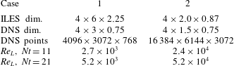Following the progressive imposition of a constant mean density gradient, $\text{d}\bar{{\it\rho}}/\text{d}z$ with gravitational acceleration $g$ , the wake flow field develops freely such that the mean velocity profile evolves according to the power laws observed in the laboratory (Spedding Reference Spedding1997, Reference Spedding2002). The spatial discretization of the numerical solution relies on a Fourier pseudospectral method in the horizontal directions and on a spectral multidomain penalty method based on Legendre polynomials in the vertical (Diamessis, Domaradzki & Hesthaven Reference Diamessis, Domaradzki and Hesthaven2005). Numerical stability is maintained by the penalty method and by spectral filtering in all three spatial directions. It is this spectral filter that serves as a surrogate for a subgrid scale model in the ILES. As needed, the wake is gradually interpolated onto a larger domain with a coarser grid to accommodate the propagation of internal waves radiating from the turbulent core and also to prevent spurious interactions with the wake’s spanwise periodic counterpart. The domain dimensions, and the Reynolds numbers for the cases and times considered, are given in table 1.

Table 1.

Simulation parameters; dimensions are in metres. The diameter and tow speed of the reference sphere are $D=0.15$  m and $U=0.0336~\text{m}~\text{s}^{-1}$ . The Reynolds number in the simulations is changed by adjusting the kinematic viscosity ${\it\nu}$ . Here $Re_{L}=u^{\prime }L/{\it\nu}$ , where $u^{\prime }$ and $L$ are the centreline r.m.s. axial velocity and the longitudinal integral scale of the axial velocity, respectively. The Prandtl number, $Pr={\it\nu}/{\it\kappa}$ where ${\it\kappa}$ is the mass diffusivity, is taken to be 1 in the DNS.

To initialize the DNS, snapshots of the ILES are taken at $Nt=9$ and 19, and interpolated onto uniformly spaced grids with dimensions given in table 1. Here $t$ is time, $N=\sqrt{-(g/{\it\rho}_{0})(\text{d}\bar{{\it\rho}}/\text{d}z)}$ is the buoyancy frequency and ${\it\rho}_{0}$ a constant reference density. The times shown in the table are the end times after the snapshot has been advanced in time for $Nt=2$ using the fully periodic pseudospectral scheme described in Hebert & de Bruyn Kops (Reference Hebert and de Bruyn Kops2006). The resolution of the DNS is such that the maximum wavenumber (after dealiasing) times ${\it\eta}$ is at least 3.0. This criterion is shown in de Bruyn Kops (Reference de Bruyn Kops2015) and the references therein to enable accurate local small-scale quantities and converged statistics of at least the fourth-order moments of the velocity and scalar fluctuations. The DNS are advanced in time for $Nt=2$ because it is observed that all terms in the enstrophy equation are quasi-stationary (in the sense that the wake evolves in time) within $Nt=1.5$ after the time the DNS is started.

3 Detection of the T/NT interface

For non-stratified flows, for which the T/NT interface is defined as that separating strong vortical from irrotational flow, many methods have been used to set a threshold value for vorticity magnitude that can then be used to determine the interface. For example, Taveira et al. (Reference Taveira, Diogo, Lopes and da Silva2013) have computed the total volume of a turbulent region as a function of the vorticity threshold ${\it\omega}_{th}$ . They found that a plateau exists in the total volume for a range of values of ${\it\omega}_{th}$ . By examining the turbulent region graphically, they found very little variation in the location of the T/NT interface as the threshold was varied throughout this range; this implied that the vorticity threshold could be located in this range, and the threshold could be used in determining the T/NT interface. This technique has since been employed successfully to detect the T/NT interface in studies using direct numerical simulation of planar turbulent jets (Watanabe et al. Reference Watanabe, Sakai, Nagata, Ito and Hayase2014) and turbulent mixing layers (Attili, Cristancho & Bisetti Reference Attili, Cristancho and Bisetti2014).

We here extend this method of identifying the T/NT interface to stably stratified flows by using, in addition to vorticity, the potential vorticity defined as ${\it\Pi}=\boldsymbol{{\it\omega}}\cdot \boldsymbol{{\rm\nabla}}{\it\rho}$ , where $\boldsymbol{{\it\omega}}$ is the vorticity and ${\it\rho}$ is the density. Potential vorticity satisfies the equation

(3.1) $$\begin{eqnarray}\frac{\text{D}{\it\Pi}}{\text{D}t}=\frac{1}{Re}\frac{\partial }{\partial x_{k}}\biggl(g_{i}\frac{\partial {\it\omega}_{i}}{\partial x_{k}}+\frac{1}{Pr}{\it\omega}_{i}\frac{\partial g_{i}}{\partial x_{k}}\biggr)-\frac{1}{Re}\biggl(1+\frac{1}{Pr}\biggr)\frac{\partial {\it\omega}_{i}}{\partial x_{k}}\frac{\partial g_{i}}{\partial x_{k}}\,,\end{eqnarray}$$

where $g_{i}\equiv \partial {\it\rho}/\partial x_{i}$ and $\text{D}/\text{D}t$ is the usual substantial derivative. Here the equation has been non-dimensionalized using the sphere diameter $D$ , tow speed $U$ and a reference density ${\it\rho}_{r}=-D(\text{d}\overline{{\it\rho}}/\text{d}z)$ . Neglecting viscous and diffusive effects, ${\it\Pi}$ is conserved following the flow. This implies that, in a turbulent region for which the external flow is initially irrotational, the irrotational flow can only obtain potential vorticity by viscous and diffusive effects, and in particular not by internal wave propagation. The internal wave region outside the turbulent wake, therefore, although it contains vorticity through the propagation of the internal waves, can contain no potential vorticity.

Figure 1.

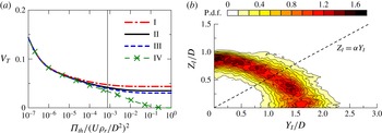
(a) Dependence of volume fraction of turbulent regions $V_{T}$ on the threshold ${\it\Pi}_{th}$ calculated at $Nt=21$ (Case 1) for (I) ${\it\omega}_{th}=0.05\langle {\it\omega}^{2}\rangle$ , (II) ${\it\omega}_{th}=0.1\langle {\it\omega}^{2}\rangle$ , (III)  ${\it\omega}_{th}=0.15\langle {\it\omega}^{2}\rangle$ and (IV) ${\it\omega}_{th}=\infty$ , where $\langle {\it\omega}^{2}\rangle$ is used as a reference value, with $\langle \cdot \rangle$ indicating the average along the centreline of the wake. The thresholds ${\it\omega}_{th}=0.1\langle {\it\omega}^{2}\rangle$ and ${\it\Pi}_{th}=0.023\langle {\it\Pi}^{2}\rangle$ are used for detecting turbulent regions. The vertical solid line in the figure indicates the threshold ${\it\Pi}_{th}=0.023\langle {\it\Pi}^{2}\rangle$ . (b) Joint p.d.f. of the location of the wake edge $(Y_{I},Z_{I})$ at $Nt=21$ for Case 1. The broken line in panel (b) shows $Z_{I}={\it\alpha}Y_{I}$ , where ${\it\alpha}=\langle Z_{I}\rangle /\langle Y_{I}\rangle$ is the aspect ratio defined by the mean locations of the wake edges $\langle Y_{I}\rangle$ at $z=0$ and $\langle Z_{I}\rangle$ at $y=0$ .

Thresholds are simultaneously applied for both the vorticity squared (enstrophy) and the potential vorticity squared (potential enstrophy), and the vorticity/potential vorticity (turbulent) region is computed as a function of both thresholds. In particular, a local region is considered turbulent if either ${\it\omega}^{2}>{\it\omega}_{th}$ or ${\it\Pi}^{2}>{\it\Pi}_{th}$ . In doing so a plateau is found, as a function of both variables, where the turbulent volume is somewhat insensitive to variations in both. Figure 1(a) is a typical plot, here for Case 1 at $Nt=21$ , of the volume fraction of the turbulent region as a function of the potential enstrophy threshold for a range of enstrophy thresholds. It is seen that indeed a significant plateau region does exist. Using this approach the core regions of the wake are detected by vorticity whereas the wake edge is detected by potential vorticity. The wake edge identified based on the thresholds is located within the T/NT interface layer, and is used for investigating the flows near the interface.

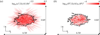
Figure 1(b) gives the joint probability density (p.d.f.) function of the location of the wake edge on cross-sectional ( $y$ – $z$ ) planes for the same case and time. The plot shows how the turbulent region spreads more horizontally than vertically, and gives some idea of the spatial variation of the turbulent boundary along the length of the wake. Some perspective on the enstrophy and potential enstrophy fields, along with the use of the T/NT detection criterion, can be seen in figure 2(a,b), which are cross-sectional plots of enstrophy and potential enstrophy for a typical cross-plane for this same case. In figure 2(a) giving the enstrophy, both the turbulent wake region and the internal wave region are easily identified. In figure 2(b) the potential enstrophy region is seen to be very compact, and well defined by the T/NT detection scheme.

Figure 2.

Vertical cross-sections of (a) enstrophy and (b) potential enstrophy fields at $Nt=21$ for Case 1. The solid black line shows the wake edge.

4 Results conditioned on the location of the interface

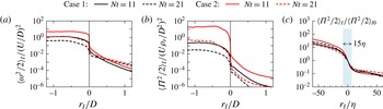
Having developed a method for detecting the T/NT interface, it is of interest to examine the behaviour of the flow properties in the vicinity of this interface. This is done by considering averages, conditioned on the location from the wake edge, $\langle \ast \rangle _{I}$ . In the results presented here, the entire interface, along the length of the wake and around its circumference, is used for conditioning. Figure 3(a,b) give plots of the conditional enstrophy and potential enstrophy, respectively, where $r_{I}=0$ is the location of the interface, $r_{I}$ positive indicates the region outside the wake and $r_{I}$ negative indicates the region inside the wake. $r_{I}$ is taken in the radial direction. The dependences of the enstrophy and potential enstrophy on the Reynolds number and on decay time are clearly visible, as well as the sharp decrease in both quantities across the interface. In addition it is seen that the potential enstrophy decays much more rapidly with distance away from the turbulent region, as expected from the discussion of (3.1).

Figure 3.

Conditional mean profiles of (a) enstrophy ${\it\omega}^{2}/2$ and (b) potential enstrophy ${\it\Pi}^{2}/2$ . (c) Conditional mean potential enstrophy ${\it\Pi}^{2}/2$ against the distance from the wake edge normalized by the Kolmogorov length scale ${\it\eta}$ . In (c), the conditional mean potential enstrophy is normalized by the value at the wake edge $\langle {\it\Pi}^{2}/2\rangle _{I0}$ at $r_{I}=0$ .

Of fundamental importance is the thickness of the interface itself. To determine this the conditional potential enstrophy, normalized by its value at the T/NT interface ( $r_{I}=0$ ), was plotted versus $r_{I}$ scaled by several potentially relevant length scales. Figure 3(c) is a plot of the conditional potential enstrophy versus $r_{I}$ scaled by the Kolmogorov length scale. The data collapse rather well, indicating that the width of the T/NT interface scales with the Kolmogorov length scale, the same result as for the non-stratified case (Watanabe et al. Reference Watanabe, Sakai, Nagata, Ito and Hayase2015). In both cases the turbulent region grows into the non-turbulent region by the diffusion of vorticity; this diffusion process depends on the fluid viscosity ${\it\nu}$ as well as on the local strain rate, of order $({\it\epsilon}/{\it\nu})^{1/2}$ , leading dimensionally to the dependence on the Kolmogorov scale ${\it\eta}=({\it\nu}^{3}/{\it\epsilon})^{1/4}$ .

Figure 4.

Conditional averaged profiles of the radial energy flux $pu_{r}$ . The line types are the same as in figure 3. The table shows values of the total kinetic energy dissipation rate ${\it\epsilon}_{T}$ and the total energy flux $F_{T}$ normalized by $U_{0}$ and $D$ .

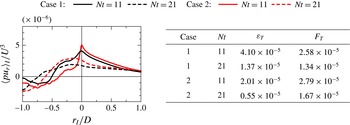
Of particular interest is the rate at which energy is being lost from the turbulent wake in the form of internal waves. Assuming the existence of internal waves, the pressure–velocity product $pu_{i}$ determines the energy flux of the internal waves in the $x_{i}$ direction. Figure 4 is a plot of the conditional radial energy flux for the four cases considered. For the early time, at $Nt=11$ , the energy flux is very similar for the two cases of different Reynolds number, indicating some insensitivity to the Reynolds number. When the kinetic energy equation is integrated over the turbulent wake region, the term ${\it\epsilon}_{T}=(1/L_{x})\int _{{\mathcal{V}}}{\it\epsilon}\,\text{d}V$ represents the rate at which kinetic energy is being lost to heat per unit length of wake, while the term $\displaystyle F_{T}=L_{p}\langle pu_{r}\rangle _{I}$ represents the conditional energy flux per unit length across the wake boundary. Here ${\mathcal{V}}$ is the wake volume, $L_{x}$ is the simulation length in the direction of the tow and $L_{p}$ is the length of the perimeter of the average cross-section of the wake, assuming that the mean wake is of approximately elliptical shape with the minor and major radii of $\langle Z_{I}\rangle$ and $\langle Y_{I}\rangle$ and the aspect ratio ${\it\alpha}$ in figure 1(b). The table in figure 4 contains the values of both ${\it\epsilon}_{T}$ and $F_{T}$ . Note that the values are very similar, especially at the later times and for the case of higher Reynolds number. These results indicate that the energy loss to internal wave radiation is of the same order as that lost due to the dissipation of kinetic energy into heat.

Figure 5.

Conditional statistics of turbulence characteristics near the wake edge: (a) Kolmogorov length scale ${\it\eta}$ , Ozmidov length scale $L_{O}$ and buoyancy Reynolds number $R_{b}$ calculated from the conditional mean dissipation rate of kinetic energy $\langle {\it\epsilon}\rangle _{I}$ at $Nt=11$ for Case 1 and (b) logarithmic plots of buoyancy Reynolds number. (c) Conditional joint p.d.f. of potential enstrophy ${\it\Pi}^{2}/2$ and the viscous/molecular-diffusion term $D_{{\it\Pi}}$ at $r_{I}/D=-0.1$ . (d) Conditional joint p.d.f. of potential enstrophy ${\it\Pi}^{2}/2$ and the production/dissipation term ${\it\epsilon}_{{\it\omega}g}$ at $r_{I}/D=-0.1$ . The results at $Nt=11$ for Case 1 are presented. In this figure, the hats denote variables normalized by $U_{0}$ , $D$ and ${\it\rho}_{r}=D(-\text{d}\overline{{\it\rho}}/\text{d}z)$ .

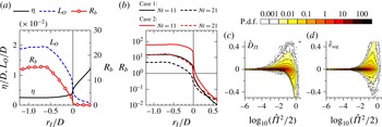
To determine the strength of the turbulence in the wake, of particular interest is the behaviour of both the Ozmidov scale $L_{O}=({\it\epsilon}/N^{3})^{1/2}$ and the Kolmogorov scale ${\it\eta}$ , and their ratio in terms of the buoyancy Reynolds number $R_{b}=(L_{O}/{\it\eta})^{4/3}={\it\epsilon}/{\it\nu}N^{2}$ . The Ozmidov scale is often interpreted as the largest horizontal scale that can overturn in a turbulent flow in a stably stratified fluid (see e.g. Riley & Lindborg Reference Riley, Lindborg, Davidson, Kaneda and Sreenivasan2013). Gibson (Reference Gibson1980) has argued that three-dimensional turbulence cannot exist when $R_{b}$ is sufficiently small. In figure 5(a) are plotted both the conditional Ozmidov and Kolmogorov length scales as well as the buoyancy Reynolds number for Case 1 at the time $Nt=11$ . Three regions are visible in the plots. First of all, in the interior of the wake, for $r_{I}/D$ less than about $-0.5$ , all three parameters are somewhat uniform, indicative of an active turbulent region. Nearer the wake edge, in the range of about $-0.5\leqslant r_{I}/D\leqslant 0$ , both the Ozmidov scale and the buoyancy Reynolds number decrease monotonically, possibly indicating the existence of internal waves as well as turbulence. At about the wake edge, the Ozmidov and Kolmogorov scales become about equal, indicating the suppression of the turbulence at the wake edge. The buoyancy Reynolds number is then effectively zero outside the wake. The values of the buoyancy Reynolds number are plotted for all four cases in figure 5(b). Again the dependences on the Reynolds number and the decay time are clearly evident. At the earlier times, and at later times for Case 2, $R_{b}$ is sufficiently large inside the wake, above a value of about 20 (Rohr et al. Reference Rohr, Itsweire, Helland and Van Atta1988; Ivey & Imberger Reference Ivey and Imberger1991; Itsweire et al. Reference Itsweire, Koseff, Briggs and Ferziger1993), that the turbulence is probably actively mixing. At the later time for Case 1, however, $R_{b}$ has dropped below 10, which indicates that the flow is probably not exhibiting active mixing.

It is of interest to examine the behaviour near the T/NT interface of the potential enstrophy itself, ${\it\Pi}^{2}/2$ . For this case with $Pr=1$ , multiplying (3.1) by ${\it\Pi}$ and rearranging gives the equation for the potential enstrophy:

(4.1) $$\begin{eqnarray}\frac{\text{D}}{\text{D}t}{\it\Pi}^{2}/2=\frac{1}{Re}{\rm\nabla}^{2}{\it\Pi}^{2}/2-\frac{1}{Re}\boldsymbol{{\rm\nabla}}{\it\Pi}\boldsymbol{\cdot }\boldsymbol{{\rm\nabla}}{\it\Pi}-\frac{2}{Re}{\it\Pi}\boldsymbol{{\rm\nabla}}{\it\omega}_{i}\boldsymbol{\cdot }\boldsymbol{{\rm\nabla}}g_{i}.\end{eqnarray}$$

The first term on the right-hand side is the viscous/molecular-diffusion term, $D_{{\it\Pi}}$ , the second is the dissipation-rate term, ${\it\epsilon}_{{\it\Pi}}$ , while the third is a mixed production/dissipation term, ${\it\epsilon}_{{\it\omega}g}$ . The latter term can take on either sign. Some idea of the behaviour of these terms is found in figure 5(c,d), which give conditional joint probability density functions of $D_{{\it\Pi}}$ and ${\it\Pi}^{2}/2$ , and of ${\it\epsilon}_{{\it\omega}g}$ and ${\it\Pi}^{2}/2$ , respectively. These two figures are taken from Case 1 at $Nt=11$ , and at the location inside the wake of $r_{I}/D=-0.1$ , but are representative of plots of the same quantities at other points in the wake turbulence. From figure 5(c) one sees, in particular, that for low values of ${\it\Pi}^{2}/2$ , the fluid acquires potential enstrophy primarily by viscous/molecular diffusion. For larger values of ${\it\Pi}^{2}/2$ , potential enstrophy is both increased and decreased by viscous/molecular diffusion, but $D_{{\it\Pi}}$ tends to negative values for very large ${\it\Pi}^{2}/2$ , indicating the transport of potential enstrophy from the turbulent wake region with large ${\it\Pi}^{2}/2$ to the entrained fluid with small ${\it\Pi}^{2}/2$ . From figure 5(d) one sees that the joint production/dissipation term ${\it\epsilon}_{{\it\omega}g}$ , representing the effects of molecular diffusion on the alignment of ${\it\omega}_{i}$ and $\boldsymbol{{\rm\nabla}}{\it\rho}$ , takes on both positive and negative values, is effective at larger values of ${\it\Pi}^{2}/2$ and has a preference for positive values.

Since the isosurface of potential enstrophy is used for detecting the wake edge, the local entrainment velocity $v_{e}$ (Holzner & Lüthi Reference Holzner and Lüthi2011) is obtained as the propagation velocity of the isosurface, $v_{e}=(\text{D}{\it\Pi}^{2}/\text{D}t)/|\boldsymbol{{\rm\nabla}}{\it\Pi}^{2}|$ . We find that the average value of $v_{e}$ is very near zero for all four cases. Average entrainment velocities of the order of the Kolmogorov velocity have been found in non-stratified shear flows (Wolf et al. Reference Wolf, Holzner, Lüthi, Krug, Kinzelbach and Tsinober2013; Watanabe et al. Reference Watanabe, da Silva, Yasuhiko, Nagata and Hayase2016). It appears that, for these later times in the wake (2–3 buoyancy periods), the stratification is inhibiting entrainment across the T/NT interface.