



1. Introduction
The Blasius solution is one of the most remarkable solutions in fluid mechanics. It describes the steady, two-dimensional laminar boundary layer that forms over a semi-infinite flat plate held parallel to a constant unidirectional flow. While surprisingly accurate for many engineering purposes, the Blasius solution is only an approximate (first-order) solution, as it predicts a non-zero normal velocity at the outer edge of the boundary layer, which is physically inconsistent with the outer flow assumptions. In spite of this shortcoming, the Blasius solution remains a valuable asset as a benchmark for validating numerical simulations of boundary layer flows and as the base flow profile for boundary layer stability analysis. It must be emphasised that the steady Blasius boundary layer is physically unstable via different mechanisms such as Tollmien–Schlichting waves; the present work does not attempt to predict transition, but rather focuses strictly on the exact mathematical structure of the steady adjoint boundary layer equations.
Linearised perturbations to a Blasius boundary layer have been considered in many contexts. The most relevant to us is the work of Libby & Fox (Reference Libby and Fox1963), who identified an infinite tower of two-dimensional (steady) perturbation modes, and obtained the discrete eigenvalues and eigenfunctions of the perturbation equation, and applied them to the analysis of first-order boundary layer solutions deviating slightly from the Blasius solution. Subsequent work clarified the mathematical problem, provided more eigenvalues, and derived approximate and asymptotic formulae for the eigenvalues. A comprehensive review of those early developments can be found in Libby (Reference Libby1970). More recent work has generalised the Libby–Fox eigenmodes to more complex scenarios (Luchini Reference Luchini1996, Reference Luchini2000; Hewitt & Duck Reference Hewitt and Duck2018).
One of the interesting features of the Libby–Fox analysis is that it is possible to develop a Green’s function solution that will enable us to directly link the perturbative and adjoint approaches. Adjoint equations have many applications across mathematics, engineering and the sciences. Of particular interest to us are applications related to adjoint-based sensitivity analysis (Peter & Dwight Reference Peter and Dwight2010), where adjoint techniques are highly efficient in determining the sensitivity of output quantities (such as lift and drag) to a large number of input data variables. This interpretation is at the heart of most engineering applications of adjoint techniques in fluid dynamics, including flow stability (Luchini & Bottaro Reference Luchini and Bottaro2014), aerodynamic design (Jameson Reference Jameson1988; Giles & Pierce Reference Giles and Pierce2000), flow control (Lions Reference Lions1971; Liu & MacArt Reference Liu and MacArt2024) and error estimation (Fidkowski & Darmofal Reference Fidkowski and Darmofal2011). Another interpretation, more technical in nature but directly related to the previous one, will be of primary concern here: the adjoint variable at a specific location is precisely the value of the linearised objective function evaluated with the appropriate Green’s function of the original problem (Giles & Pierce Reference Giles and Pierce2001). This link with the Green’s function has been used to obtain exact adjoint solutions (Lozano & Ponsin Reference Lozano and Ponsin2022) and will be exploited here for the analysis of the adjoint solution to the boundary layer equations.
Adjoint methods have been applied to boundary layer flows in a variety of contexts. The adjoints of the Navier–Stokes, parabolised stability, Orr–Sommerfeld or boundary layer equations have been used in shape optimisation, flow control, boundary layer stability, adjoint-based global-mode stabilisation, boundary layer receptivity, structural sensitivity, identification of optimal perturbations and resolvent analysis. The literature is too vast to be properly summarised here, but Luchini & Bottaro (Reference Luchini and Bottaro2014) contains a comprehensive overview of adjoint applications to hydrodynamic stability up to 2014.
Directly related to the present paper is the recent work by Kühl et al. (Reference Kühl, Müller and Rung2021), where a thorough analysis of the complete adjoint boundary layer equations and dynamics is presented, including a proposal for an analytic adjoint solution for the Blasius boundary layer. It also contains the intriguing idea that the adjoint solution develops a boundary layer structure that emanates from the end of the plate, as corresponds to the reversed convective characteristics relative to the primal flow. Their analysis differs from ours in several aspects, and their proposed solution appears to be in conflict with the solution that we will present below except under special circumstances.
The present paper explicitly casts the solution to the adjoint of the Prandtl boundary layer equations on a flat plate as a Libby–Fox eigenfunction expansion, and discusses its convergence properties. The restricted scope of the paper poses a clear limitation of this work, its direct relevance to more complex geometries, unsteady perturbations or fully turbulent flows being debatable. On the other hand, an improved understanding of the adjoint solution corresponding to the Blasius boundary layer is relevant in several regards. First, even though assembling the solution requires significant numerical work, it can be used as a validation case for adjoint Navier–Stokes or boundary layer solvers, and can also help to guide the proper formulation of the adjoint problem and its boundary conditions in numerical implementations. In this regard, sample solutions for the Blasius and Falkner–Skan cases (with pressure gradient parameter
 $\beta =1/2$
) are collected in two tables in Appendix F. The solution can also be used to understand the mathematical structure of the adjoint problem in a simplified, yet fundamental, case.
Likewise, an analytic solution facilitates theoretical developments, such as deriving constraints on the eigenvalues and eigenfunctions of the primal problem, and analysing the adjoint transpose convection (ATC) term, whose actual value is hard to determine from the viewpoint of the original partial differential equations. Finally, an explicit adjoint solution can be used to directly compute gradients and sensitivities with respect to various control parameters such as initial velocity profiles, plate shape and wall-normal velocity distributions.
To make the subject as accessible as possible, the paper is organised as follows. Section 2 reviews some basic facts about the Libby–Fox analysis of perturbations to the Blasius solution. Section 3 introduces the adjoint equations and derives the adjoint eigenvalue problem. Section 4 applies the Green’s function approach to compute the semi-analytic adjoint solution. The solution is shown to obey the adjoint boundary conditions, and the possibility that it can be written in a simple similarity form is explicitly refuted. Section 5 presents some numerical experiments, including sample solutions evaluated from numerical integration of the adjoint Libby–Fox equation, and presents empirical convergence properties and comparisons with numerical solutions obtained by discretising the adjoint equations directly. Section 6 applies the analytic solution to the analysis of the ATC term, and to the sensitivity analysis of the drag coefficient in initial-value, shape design and active flow control (via blowing–suction) problems. Section 7 briefly examines the extension to Falkner–Skan flows. Section 8 summarises the findings of the paper and outlines future research.
2. Perturbations to the boundary layer equations
This section contains a brief review of some well-known facts about linearised perturbations to the Blasius boundary layer solution as originally developed by Libby & Fox (Reference Libby and Fox1963). There is much more to say about this topic than can be found here. Aside from the original reference, Libby (Reference Libby1970) contains an excellent review, and we also found the introduction in Luchini (Reference Luchini1996) particularly useful.
The equations for the incompressible boundary layer along a flat plate with zero pressure gradient are
 \begin{align} u u_x + v u_y - \nu u_{yy} &= 0,\nonumber\\ u_x + v_y &= 0, \end{align}
where
 $(x,y)$
are Cartesian coordinates chosen such that the plate extends along the positive
 $x$
axis,
 $(u,v)$
are the Cartesian components of the velocity, and
 $\nu$
is the constant (kinematic) viscosity. In (2.1) and in the remainder of the paper, we will denote derivatives by subscripts, so
 $u_y = \partial _y u$
. Equation (2.1) can be equivalently written in terms of a streamfunction
 $\psi (x,y)$
as
 \begin{equation} \psi _y \psi _{xy} - \psi _x \psi _{yy} - \nu \psi _{yyy}=0, \end{equation}
where
 $\psi (x,y)$
is related to the velocity as
 $(u,v) = (\psi _y, -\psi _x)$
.
An equivalent equation describing the boundary layer can be obtained by changing variables to
 $\psi (x,y) = \sqrt {2 \textit{Re}_m\, \nu ^2 x}\, F(x,\eta )$
, where
 $\eta = y \sqrt {\textit{Re}_m / (2x)}$
is the Blasius similarity variable,
 $\textit{Re}_m = \rho U / \mu = U / \nu$
is the Reynolds number per unit length (Reynolds number per metre), and
 $\mu$
,
 $\rho$
and
 $U$
are the viscosity, density and velocity at the edge of the boundary layer, respectively. With these definitions, (2.2) is transformed into
 \begin{equation} F_{\eta \eta \eta }(x,\eta ) + F(x,\eta )\, F_{\eta \eta }(x,\eta ) = 2x \left (F_\eta (x,\eta )\, F_{x\eta }(x,\eta ) - F_{\eta \eta }(x,\eta )\, F_x(x,\eta )\right ), \end{equation}
where now
 $x$
and
 $\eta$
have to be understood as formally independent variables. Equation (2.3) admits the particular solution
 $ F(x,\eta ) = F_0(\eta )$
, where
 $F_0$
is the Blasius similarity function obeying
 \begin{equation} F_{0,\eta \eta \eta }(\eta ) + F_0(\eta )\, F_{0,\eta \eta }(\eta ) = 0, \end{equation}
with
 $F_0(0) = 0$
,
 $F_{0,\eta }(0) = 0$
and
 $F_{0,\eta }(\infty ) = 1$
. Libby and Fox investigated non-similar solutions to (2.3) of the form
 $F(x,\eta ) = F_0(\eta ) + \delta\, F(x,\eta )$
, where
 $\delta F$
is a small perturbation. The equation for
 $\delta F$
is obtained by linearising (2.3) about
 $F_0$
, and is
 \begin{equation} \delta F_{\eta \eta \eta } + F_0\, \delta F_{\eta \eta } + F_{0,\eta \eta }\, \delta F + 2x (F_{0,\eta \eta }\, \delta F_x - F_{0,\eta }\, \delta F_{x\eta }) = 0. \end{equation}
Equation (2.5) has separable solutions of the form
 \begin{equation} \delta F(x,\eta ) = x^{-\lambda /2}\, N(\eta ), \end{equation}
where the functions
 $N$
are solutions to the eigenvalue problem
 \begin{equation} N_{\eta \eta \eta } + F_0 N_{\eta \eta }+ \lambda F_{0,\eta } N_\eta +(1- \lambda ) F_{0,\eta \eta } N = 0, \end{equation}
with the conditions
 $N(0)=0$
,
 $N_\eta (0)=0$
,
 $N_\eta (\infty )=0$
as well as the scaling condition
 $N_{\eta \eta }(0)=1$
.
Imposing the additional condition that
 $N_\eta$
vanishes exponentially fast at infinity allowed Libby and Fox to transform the eigenvalue problem (2.7) into a second-order Sturm–Liouville equation:
 \begin{equation} \left ( \frac {F_{0,\eta }^3}{F_{0,\eta \eta }} H_{\eta } \right )_\eta + \lambda \frac {F_{0,\eta }^4}{F_{0,\eta \eta }} H - F_0 F_{0,\eta }^2 H = 0, \end{equation}
where
 $H = (N/F_{0,\eta })_\eta$
. Consequently, the eigenvalues form an infinite discrete sequence of positive real numbers
 $\lambda _k \gt 0$
,
 $k=1,2,\ldots$
, and the eigenfunctions form a complete orthogonal set obeying
 \begin{equation} \int _0^\infty \frac {F_{0,\eta }^4}{F_{0,\eta \eta }} \left (\frac {N_k}{F_{0,\eta }}\right )_\eta \left (\frac {N_j}{F_{0,\eta }}\right )_\eta {\rm d}\eta = \delta _{kj} C_k, \end{equation}
and can be used to represent any physically admissible perturbation to the Blasius boundary layer.
The first eigenvalue can be determined exactly as
 $\lambda _1 = 2$
, and its corresponding eigenfunction is
 \begin{equation} N_1 = (\eta F_{0,\eta } - F_0)/\alpha, \end{equation}
where
 $\alpha = F_{0,\eta \eta }(0)$
, such that
 $N_1/x$
is a solution to (2.5) that corresponds to a simple translation of the origin of coordinates (Stewartson 1957). The higher (
 $k\gt 1$
) eigenvalues and eigenfunctions are hard to obtain, and are only amenable to numerical treatment. The next few eigenvalues are 3.774, 5.629, 7.513, so that the general solution has the form
 \begin{equation} \begin{aligned} \delta F(x,\eta ) &= \sum _{k=1}^\infty A_k x^{-\lambda _k/2}\, N_k(\eta ) \\ &= A_1 x^{-1} (\eta F_{0,\eta } - F_0)/\alpha + A_2 x^{-1.887} N_2 + A_3 x^{-2.814} N_3 + A_4 x^{-3.757} N_4 + \cdots. \end{aligned} \end{equation}
The eigenvalue problem (2.7) is singular in that the boundary conditions, alone, are not sufficient to determine the spectrum. Determination of the spectrum requires imposing on the eigenfunctions an exponential decay at infinity. A variety of techniques has been used to determine the eigenvalues and eigenfunctions of (2.7) (see Libby (Reference Libby1970) for a review of early developments). The original work of Libby & Fox (Reference Libby and Fox1963) only gave the first 10 eigenvalues. Libby (Reference Libby1965), Wilks & Bramley (Reference Wilks and Bramley1977) and Luchini (Reference Luchini1996) listed the first twenty eigenvalues. These are all exact approaches. The Libby–Fox and Luchini approaches are based on the matching of a forward integration (
 $\eta$
increasing) of the full equation (2.7) with a backward integration (
 $\eta$
decreasing) of the asymptotic form of (2.7), while the Wilks and Bramley approach is based on a Riccati transformation of the perturbation equations (Wilks Reference Wilks1979).
On the other hand, Kotorynski (Reference Kotorynski1968) derived approximate values for the eigenvalues replacing the coefficient functions of (2.7) by the sum of its asymptotic terms near the wall and far from the wall. Kemp (Reference Kemp1970) improved the Kotorynski formula, giving approximate values for the norms as well, and additionally applied the results of a WKB approximation to obtain a more accurate approximation for the eigenvalues. Finally, Brown (Reference Brown1968), using matched asymptotic expansions, obtained the following asymptotic formula for the eigenvalues:
 \begin{equation} \lambda _k = 2(k-1) - 0.2705\sqrt {2(k-1)} + 2.203 - \frac {0.076}{\sqrt {2(k-1)}} + \mathcal{O}\left (\frac {1}{2(k-1)}\right ) \end{equation}
(valid for
 $k\gt 1$
), which works surprisingly well, yielding a relative error of 0.18 % already at
 $k=2$
.
3. Adjoint boundary layer problem formulation
There are several ways to define the adjoint equations associated with the Blasius solution. One can consider the adjoint to the full Navier–Stokes equations about the Blasius solution, the adjoint to the boundary layer equations, or finally, the adjoint to Prandtl’s boundary layer equations for the flat plate (2.1). We will consider the last option. The corresponding derivation of the adjoint equations and boundary conditions has been discussed at length in Kühl et al. (Reference Kühl, Müller and Rung2021) and will not be repeated here.
The application of the adjoint approach in sensitivity analysis is based on the premise that one wishes to compute the sensitivity of a certain quantity of interest or objective function to flow perturbations. This can be done directly by solving the linearised flow equations. However, if the number of perturbations is large (as in e.g. a shape design problem with many design variables), then the cost soon becomes prohibitive. The adjoint approach is designed to bypass the need to compute the linearised flow equations for each independent perturbation, requiring instead the solution of a single partial differential equation for each independent objective function.
In the present case, the selected objective function is the integrated friction drag coefficient along a section of length
 $L$
of the plate, which is defined as
 \begin{equation} C_D(L) = \tilde {\kappa } \int _0^L (u_y)_{y=0} {\rm d}x, \end{equation}
where
 $\tilde {\kappa } = 2\mu /(\rho U^2 L) = 2/(\textit{Re}_m L U)$
is a normalisation constant. Rewriting (3.1) in terms of the streamfunction, and using a Lagrange multiplier
 $\tilde {\psi }$
to enforce the flow equation (2.2), yields the Lagrangian
 \begin{equation} \mathcal{L} = \tilde {\kappa } \int _0^L (\psi _{yy})_{y=0} {\rm d}x - \int _0^L \int _0^\infty \tilde {\psi } (\psi _y \psi _{xy} - \psi _x \psi _{yy} - \nu \psi _{yyy})\, {\rm d}x {\rm d}y. \end{equation}
Equation (3.2) sets the basis for the adjoint treatment and also helps to fix notation as well as the normalisation of the adjoint field
 $\tilde {\psi }$
. Notice that by using the streamfunction formulation, there is no need to add to (3.2) a term to enforce the incompressibility condition.
Linearising (3.2) with respect to flow perturbations
 $\delta \psi$
, integrating by parts and rearranging yields
 \begin{equation} \begin{aligned} \delta \mathcal{L} = \delta C_D(L) &= \tilde {\kappa } \int _0^L (\delta \psi _{yy})_{y=0}\, {\rm d}x \\ &\quad - \int _0^L \int _0^\infty \delta \psi\, (\psi _y \tilde {\psi }_{xy} - \psi _x \tilde {\psi }_{yy} - 2\psi _{xy} \tilde {\psi }_y + 2\psi _{yy} \tilde {\psi }_x + \nu \tilde {\psi }_{yyy})\, {\rm d}x {\rm d}y \\ &\quad + \int _0^L {\rm d}x\, \big[ \tilde {\psi } \psi _x\, \delta \psi _y - 2\tilde {\psi } \psi _{xy}\, \delta \psi - \tilde {\psi }_y \psi _x\, \delta \psi - \tilde {\psi } \psi _y\, \delta \psi _x\big]_{y=0}^{y=\infty } \\ &\quad + \int _0^L {\rm d}x\, \big[ \nu \tilde {\psi }\, \delta \psi _{yy} - \nu \tilde {\psi }_y\, \delta \psi _y + \nu \tilde {\psi }_{yy}\, \delta \psi \big]_{y=0}^{y=\infty } \\ &\quad + \int _0^\infty{\rm d}y\, \big[ \tilde {\psi }_y \psi _y\, \delta \psi + 2\tilde {\psi } \psi _{yy}\, \delta \psi \big]_{x=0}^{x=L}. \end{aligned} \end{equation}
For design applications, (3.3) contains an additional term that corresponds to the perturbation of the plate geometry. This term does not play any role in the derivation of the adjoint equations and is not included here, but it will be briefly discussed in § 6.2.
The adjoint problem is defined to eliminate the dependence of (3.3) on
 $\delta \psi$
and its derivatives so that the sensitivity of the cost function to flow perturbations can be computed without having to solve the linearised perturbation equation. Vanishing of the domain integral requires that
 $\tilde {\psi }$
obeys the adjoint equation
 \begin{equation} \psi _y \tilde {\psi }_{xy} - \psi _x \tilde {\psi }_{yy} - 2\psi _{xy} \tilde {\psi }_y + 2\psi _{yy} \tilde {\psi }_x + \nu \tilde {\psi }_{yyy} = 0. \end{equation}
The boundary terms are tackled in a similar fashion. In some of them,
 $\delta \psi$
and its derivatives cannot be computed without solving the linearised flow equations. Others are completely specified by the linearised boundary conditions. The former are eliminated by imposing the following boundary conditions on the adjoint variable:
 \begin{align} \tilde {\psi }(x,0) = \frac {\tilde {\kappa }}{\nu } &= \frac {2}{L U^2},\nonumber\\ \tilde {\psi }(L,y) &= 0,\nonumber\\ \tilde {\psi }(x,\infty ) &= 0. \end{align}
The remaining boundary terms yield the sensitivity derivatives. We will use some of them in § 6.
It may be useful at this stage to compare (3.4) to more conventional adjoint treatments. Equation (3.4) is a single, third-order equation for one adjoint variable, when in view of (2.1) one would expect two adjoint variables obeying two equations of second order at most. In fact, the adjoint equations corresponding to (2.1) can be easily shown to be
 \begin{align} \tilde {\psi }_{p,x} + u \tilde {\psi }_x + v \tilde {\psi }_y - \tilde {\psi } u_x + \nu \tilde {\psi }_{yy} &= 0,\nonumber\\ \tilde {\psi }_{p,y} - \tilde {\psi } u_y &= 0, \end{align}
where
 $\tilde {\psi }_p$
is the adjoint variable (the Lagrange multiplier) that corresponds to the continuity equation (usually known as the adjoint pressure). This
 $\tilde {\psi }_p$
can be eliminated from (3.6) by applying
 $\partial _y$
to the first equation,
 $\partial _x$
to the second, and subtracting the second equation from the first. The resulting equation, after setting
 $(u,v) = (\psi _y, -\psi _x)$
, is precisely (3.4). Once (3.4) is solved,
 $\tilde {\psi }_p$
can be obtained from (3.6).
We now change variables to
 $(x,\eta )$
, and write
 $\psi (x,y) = \sqrt {2 \textit{Re}_m\, \nu ^2 x}\, F(x,\eta )$
. In the new variables, the drag can be computed as
 \begin{equation} C_D(L) = \kappa \int _0^L \frac {1}{\sqrt {2x}} F_{\eta \eta }(x,0)\, {\rm d}x, \end{equation}
where
 $\kappa = 2/(\sqrt {\textit{Re}_m} L)$
, and the penalty term in (3.2) gets converted to
 \begin{align} & \int _0^L \int _0^\infty \tilde {\psi } (\psi _y \psi _{xy} - \psi _x \psi _{yy} - \nu \psi _{yyy})\, {\rm d}x {\rm d}y\nonumber\\&\quad = \iint {\rm d}x {\rm d}\eta \tilde {\varPsi } \big ( F_{\eta \eta \eta } + \textit{FF}_{\eta \eta } - 2x(F_\eta F_{x\eta } - F_{\eta \eta } F_x) \big ), \end{align}
where
 \begin{equation} \tilde {\varPsi }(x,\eta ) = - \frac {U^2}{\sqrt {2 \textit{Re}_m\, x}} \tilde {\psi }(x,\eta ) \end{equation}
is the adjoint variable in the new formulation. Setting
 $F = F_0 + \delta F$
in (3.8), where
 $F_0(\eta )$
is the Blasius solution, linearising with respect to the small perturbation
 $\delta F$
, and integrating by parts in
 $x$
and
 $\eta$
, yields the adjoint equation
 \begin{equation} -\tilde {\varPsi }_{\eta \eta \eta } + F_0 \tilde {\varPsi }_{\eta \eta } - 2x F_{0,\eta } \tilde {\varPsi }_{x\eta } - 4x F_{0,\eta \eta } \tilde {\varPsi }_x - 2F_{0,\eta \eta } \tilde {\varPsi } = 0, \end{equation}
with boundary conditions
 \begin{equation} \tilde {\varPsi }(x,0) = - \frac {\kappa }{\sqrt {2x}},\quad \tilde {\varPsi }(L,\eta ) = 0,\quad \tilde {\varPsi }(x,\infty ) = 0. \end{equation}
Consider the solution for
 $\tilde {\varPsi }(x,\eta )$
. Separation of variables so that
 $\tilde {\varPsi }(x,\eta ) = x^{\lambda /2-1}\,D(\eta )$
yields
 \begin{equation} -D_{\eta \eta \eta } + F_0 D_{\eta \eta } + (2 - \lambda ) F_{0,\eta } D_\eta + 2(1 - \lambda ) F_{0,\eta \eta } D = 0, \end{equation}
which happens to be adjoint to the flow eigenvalue problem (2.7). The solution to (3.12) can be found by exploiting the underlying Sturm–Liouville structure of the Libby–Fox problem. As shown in § 2, the third-order primal equation for
 $N$
(2.7) can be transformed into a Sturm–Liouville equation (2.8) for the auxiliary variable
 $H(\eta )$
. Both equations are related by an overall weight
 $W=F_{0,\eta \eta }/F_{0,\eta }^2$
. Since the Sturm–Liouville equation is formally self-adjoint, a standard continuous adjoint argument shows that if
 $H_k$
is an eigensolution with eigenvalue
 $\lambda _k$
, then
 $D_k(\eta )=H_k/W$
is an eigensolution of the adjoint equation with the same eigenvalue. Hence
 \begin{equation} D_k(\eta ) = \frac {1}{C_k} \frac {F_{0,\eta }^2}{F_{0,\eta \eta }} H_k(\eta ) = \frac {1}{C_k} \left ( \frac {F_{0,\eta }}{F_{0,\eta \eta }} N_{k,\eta } - N_k \right ), \end{equation}
where
 $C_k$
(the square of the norm of the
 $k$
th Libby–Fox eigenfunction) has been inserted for future convenience. Using the explicit representation given by (3.13), it is easy to see that
 $D_k$
obeys the third-order equation (3.12) for
 $\lambda =\lambda _k$
. We can also deduce that the adjoint eigenfunctions diverge polynomially as
 $\eta \rightarrow \infty$
(see Appendix B), while at the wall, they obey the boundary conditions
 $D_k(0) = 0$
,
 $D_{k,\eta }(0) = 0$
,
 $D_{k,\eta \eta }(0) = 1/C_k$
.
Likewise, substituting (3.13) into (2.8), it is straightforward to verify that the adjoint eigenfunctions
 $D_k$
obey the Sturm–Liouville equation
 \begin{equation} \left ( \frac {F_{0,\eta \eta }}{F_{0,\eta }} D_{k,\eta } \right )_\eta + (\lambda _k - 1) F_{0,\eta \eta } D_k = 0. \end{equation}
Hence the adjoint eigenfunctions form a complete set and are mutually orthogonal with respect to the weight
 $F_{0,\eta \eta }$
:
 \begin{equation} \int _0^\infty F_{0,\eta \eta } D_k D_j {\rm d}\eta = C_k^{-1} \delta _{kj}, \end{equation}
where the normalisation constant is inherited directly from (2.9). Likewise, the full adjoint solution can be represented as an infinite sum over
 $D_k$
. The coefficients of the modes must be fixed from the adjoint boundary conditions, which may prove to be a formidable task. Instead, we will determine them in the next section using the Green’s function approach.
4. Analytic adjoint solution from the Green’s function approach
It is a well-established fact that the adjoint variable at a particular point is equal to the value of the corresponding linearised cost function evaluated using the Green’s function for the same point (Giles & Pierce Reference Giles and Pierce2001). Libby & Fox (Reference Libby and Fox1963) found that the Green’s function that corresponds to (2.5) is
 \begin{equation} G(x',\eta '; x,\eta ) = -\mathcal{H}(x'-x) \sum _{k=1}^\infty \frac {D_k(\eta )}{2x} \left (\frac {x'}{x}\right )^{-\lambda _k/2} N_k(\eta '), \end{equation}
where
 $\mathcal{H}$
is the Heaviside function. As explained above, the adjoint variable
 $\tilde {\varPsi }$
at
 $(x,\eta )$
is equal to the linearised drag associated with the Green’s function (4.1). Using (3.7), we have
 \begin{equation} \tilde {\varPsi }(x,\eta ) =\int _0^L \frac {\kappa }{\sqrt {2x'}} G_{\eta '\eta '}(x',\eta '; x,\eta )_{\eta '=0}{\rm d}x'. \end{equation}
Inserting (4.1) into (4.2), integrating over
 $x$
and rearranging yields
 \begin{equation} \tilde {\varPsi }(x,\eta ) = \frac {\kappa }{\sqrt {2x}} (\varphi (\xi ,\eta ) - 1), \end{equation}
where
 \begin{equation} \varphi (\xi ,\eta ) = \sum _{k=1}^\infty \frac {D_k(\eta )}{\lambda _k - 1} \xi ^{\tfrac{\lambda _k - 1}{2}} \end{equation}
and
 $\xi = x/L$
. In the derivation of (4.3), we have used that
 \begin{equation} \sum _{k=1}^\infty \frac {D_k(\eta )}{\lambda _k - 1} =1, \end{equation}
a proof of which can be found in Appendix C. Equation (4.3) is the drag-based adjoint solution for the equation (2.5) describing linearised perturbations to a Blasius base state. The corresponding
 $x$
-momentum adjoint solution for the boundary layer equation (3.4) is, using (3.9),
 \begin{equation} \tilde {\psi }(x,\eta ) = \frac {2}{L U^2} \left ( 1 - \varphi (\xi ,\eta ) \right ). \end{equation}
4.1. Analysis of the adjoint boundary conditions
Let us analyse the adjoint solutions (4.3) and (4.6). It can be verified that they obey their respective adjoint equations (3.10) and (3.4). We can also verify that (4.3) obeys the adjoint boundary conditions (3.11). The constraints on (4.6) are trivially satisfied as a direct consequence.
At the plate’s end,
 $\xi =1$
, and we have
 \begin{equation} \tilde {\varPsi }(L,\eta ) = \frac {\kappa }{\sqrt {2L}} (\varphi (1,\eta ) - 1) = 0, \end{equation}
since
 $\varphi (1,\eta ) = 1$
from (4.5).
At the wall,
 $\eta = 0$
. Since
 $D_k(0) = 0$
for all
 $k$
, we have that
 $\varphi (\xi ,0) = 0$
,
 $0 \leq \xi \lt 1$
, which yields
 \begin{equation} \tilde {\varPsi }(x,0) = - \frac {\kappa }{\sqrt {2x}}, \end{equation}
as expected.
At
 $\xi = 1$
, there seems to be a contradiction since the wall boundary conditions seem to demand
 $\varphi (1,0) = 0$
, while (4.5) yields
 $\varphi (1,\eta ) = 1$
. From a physical viewpoint, this simply reflects the conflicting boundary conditions at the corner point between the outlet and the wall, and is identical to the behaviour of the Blasius function
 $F_0(y/\sqrt {x})$
as
 $x\to 0$
for
 $y\neq 0$
and
 $y=0$
.
Finally, vanishing of (4.3) at the far field
 $\eta \rightarrow \infty$
requires that
 $\lim _{\eta \rightarrow \infty } \varphi (\xi ,\eta ) = 1$
. This is demonstrated in Appendix D.
4.2. Adjoint similarity solution
A fundamental question arises regarding the similarity properties of the adjoint solution (4.6). Self-similarity of the adjoint solution would have implications for the flow sensitivities, which would be universal up to scaling, and for the structure of the Green’s function, which would likely enjoy analogous similarity properties. Since the adjoint equations are directly derived from the linearisation of the self-similar Blasius equations, one might expect the dual solution to inherit this self-similarity. If the base flow is self-similar, does the adjoint solution naturally reduce to a self-similar form as well? This question is actually very hard to answer, since it depends on the base flow, the objective function and the domain. We will therefore focus on the current setting (integrated viscous drag on a plate of finite length), and start by acknowledging a simplified system for which the answer is positive, then move on to consider the Blasius case.
Let us consider the Oseen linearisation of the boundary layer equations, which is described in more depth in Appendix A. The adjoint solution – which can be written as an eigenfunction expansion – can be put in the similarity form
 \begin{equation} \tilde {\psi }(x,y) = \frac {2}{LU^2} \left [ 1 - \mathrm{erf}\left (\frac {\hat {\eta }}{\sqrt {2}}\right ) \right ]\!, \end{equation}
where
 $\mathrm{erf}(t) = 2\pi ^{-1/2} \int _0^t \exp (-z^2)\,{\rm d}z$
is the error function, and
 $\hat {\eta } = y\sqrt {\textit{Re}_m/(2(L-x))}$
is the Blasius variable measured from the end of the plate.
Turning to the adjoint Blasius equation, if a self-similar solution existed, then it would be natural to assume that the similarity variable would be
 $\hat {\eta }$
as well. This is, in fact, the proposal of Kühl et al. (Reference Kühl, Müller and Rung2021), where it is claimed that under suitable approximations, the
 $x$
-momentum drag-based adjoint variable
 $\tilde {\psi }$
is self-similar, with similarity variable
 $\hat {\eta }$
and similarity function
 $F_{0,\eta }$
, such that
 \begin{equation} \tilde {\psi }(x,y) = \frac {2}{LU^2} [ 1 - F_{0,\eta }(\hat {\eta }) ]. \end{equation}
However, (4.10) does not obey the adjoint boundary layer equation (3.4) as can be checked by direct substitution. We can further prove this fact using the eigenfunction expansion. For the Oseen equation, the eigenfunction expansion collapses to
 $\text{erf}(\hat {\eta }/\sqrt {2})$
. For the Blasius equation, the ansatz (4.10) requires that
 \begin{equation} \sum _{k=1}^\infty \frac {D_k(\eta )}{\lambda _k - 1} \xi ^{(\lambda _k - 1)/2} = F_{0,\eta } \left ( \sqrt {\frac {\xi }{1-\xi }}\, \eta \right )\!. \end{equation}
To test (4.11), let us consider the adjoint eigenfunction expansion of
 $F_{0,\eta }(\eta )$
, i.e.
 \begin{equation} F_{0,\eta }(\eta ) = \sum _{k=1}^\infty a_k\, D_k(\eta ). \end{equation}
The coefficients
 $a_k$
can be obtained by integrating
 $F_{0,\eta }$
against the corresponding eigenfunction with the Sturm–Liouville weight
 $F_{0,\eta \eta }$
:
 \begin{equation} a_k = C_k \int _0^\infty F_{0,\eta \eta }(\eta )\, F_{0,\eta }(\eta )\, D_k(\eta )\, {\rm d}\eta. \end{equation}
We quote the results for the first 10 eigenfunctions obtained from the numerical integration of the Blasius and adjoint equations in table 1. If (4.11) held, then we could set
 $\xi = 1/2$
, and
 $F_{0,\eta }$
should obey the identity
 \begin{equation} F_{0,\eta }(\eta ) = \sum _{k=1}^\infty \frac {D_k(\eta )}{2^{(\lambda _k - 1)/2} (\lambda _k - 1)}. \end{equation}
Equality of (4.14) and (4.12) requires that
 $a_k = 2^{-(\lambda _k - 1)/2} (\lambda _k - 1)^{-1}$
. This is clearly not the case, as can be seen in table 1.
Coefficients of the adjoint eigenfunction expansion of
 $F_{0,\eta }$
.

Table 1. Long description
A table with three columns and ten rows. The columns are labeled ‘k’, ‘ak’, and ‘2^{-(λ_k-1)/2}(λ_k-1)^{-1}’. The rows present numerical values for these columns. Row 1: k, 1; ak, 0.78629152; 2^{-(λ_k-1)/2}(λ_k-1)^{-1}, 0.707106781. Row 2: k, 2; ak, 0.19995432; 2^{-(λ_k-1)/2}(λ_k-1)^{-1}, 0.137871733. Row 3: k, 3; ak, 0.09182893; 2^{-(λ_k-1)/2}(λ_k-1)^{-1}, 0.043435906. Row 4: k, 4; ak, 0.05407272; 2^{-(λ_k-1)/2}(λ_k-1)^{-1}, 0.016064568. Row 5: k, 5; ak, 0.03668328; 2^{-(λ_k-1)/2}(λ_k-1)^{-1}, 0.006434176. Row 6: k, 6; ak, 0.02716455; 2^{-(λ_k-1)/2}(λ_k-1)^{-1}, 0.002702378. Row 7: k, 7; ak, 0.02129176; 2^{-(λ_k-1)/2}(λ_k-1)^{-1}, 0.001171264. Row 8: k, 8; ak, 0.01734642; 2^{-(λ_k-1)/2}(λ_k-1)^{-1}, 0.000518991. Row 9: k, 9; ak, 0.01453172; 2^{-(λ_k-1)/2}(λ_k-1)^{-1}, 0.000233942. Row 10: k, 10; ak, 0.01239230; 2^{-(λ_k-1)/2}(λ_k-1)^{-1}, 0.000106789.
The mismatch between the coefficients rules out (4.10). This is also confirmed by direct numerical evaluation of the semi-analytic adjoint solution in § 5, which does not show similarity with respect to either
 $\hat {\eta }$
or
 $\eta$
, nor do any computations carried out to date by the authors using a variety of different Navier–Stokes solvers.
The fundamental reason that explains why the drag-based Blasius adjoint solution cannot collapse into a simple backward-facing similarity variable (or any other similarity variable) lies in the lack of translation symmetry. In the linear Oseen approximation, the constant background velocity
 $U$
makes the problem translation-invariant in
 $x$
; consequently, the adjoint solution depends solely on the distance from the trailing edge (
 $L-x$
), and a similarity variable like
 $\hat {\eta } \sim y/\sqrt {L - x}$
can be expected. The Blasius solution breaks this picture. The leading edge at
 $x = 0$
is a privileged point, and the boundary layer evolves continuously downstream. Since the adjoint equations are built around the linearisation of this base state, their coefficients explicitly depend on the distance from this origin. The adjoint equations thus have two conflicting longitudinal scales,
 $x$
and
 $L - x$
. A single similarity variable cannot simultaneously reconcile the forward-evolving flow and the backward-propagating adjoint field, precluding a self-similar collapse.
5. Numerical analysis
Here, we focus on explicitly building the adjoint solution (4.6) in order to verify its properties and to compare it to numerical adjoint solutions. The evaluation of these expressions requires the construction of the adjoint eigenfunctions and their corresponding eigenvalues and norms.
In order to build the eigenfunctions, we proceed as follows. Eigenvalues up to
 $n=20$
are taken from Luchini (Reference Luchini1996) and Wilks & Bramley (Reference Wilks and Bramley1977), while for
 $n\gt 20$
, Brown’s asymptotic relation (2.12) is used. These values are used to compute the adjoint eigenfunctions by numerical integration of either (2.7) or (3.12). The normalising constants
 $C_n$
are obtained by numerical evaluation of integrals (2.9) or (3.15). Their values are found to be reasonably well correlated by the equation
 \begin{equation} C_n \sim 1.443 n^{-0.672} \end{equation}
(or
 $C_n \sim 2.2441 \lambda _n^{-0.669}$
in terms of the eigenvalues), which compares favourably with Kemp’s approximate formula
 $C_n = 1.37 n^{-2/3}$
(Kemp Reference Kemp1970).
Using these computed eigenvalues and norms, we construct the sample solutions. Figure 1 shows the adjoint solution (4.6) computed with
 $N_{eigen} = 2800$
eigenfunctions. The solution is plotted against
 $\eta$
and
 $\hat {\eta }$
. It is clear that there is no similarity in either variable, even though the solution only depends on
 $x$
and
 $y$
through the dimensionless variables
 $\xi$
and
 $\eta$
. Notice also that
 $LU^2\tilde {\psi }/2$
seems to be bounded between 0 and 1, which means that the function
 $\varphi (\xi ,\eta )$
defined in (4.4) is also bounded between 0 and 1. We show this to be the case in Appendix D.
Approximate values of the adjoint solution
 $L U^2 \tilde {\psi }/2$
computed with 2800 eigenfunctions plotted against (a)
 $\eta$
and (b)
 $\hat {\eta }$
.

The spatial structure of the solution is actually more involved than expected. Instead of a simple boundary layer structure emanating from the trailing edge, the adjoint contours plotted in figure 2 show a parabolic-like shape peaking at approximately one-third of the plate’s length, and decaying towards the leading and trailing edges. This behaviour is likely a direct physical manifestation of the two streamwise length scales
 $x$
and
 $L-x$
that we discussed in § 4.2.
Contour levels of the adjoint solution
 $L U^2 \tilde {\psi }/2$
computed with 2800 eigenfunctions.

It is interesting to ask about the rate of convergence of the eigenfunction expansion. Libby & Fox (Reference Libby and Fox1963) pointed out the slow convergence of the expansion in various perturbation problems. Figure 3 focuses on this issue, plotting the function
 $\varphi (\xi ,\eta )$
evaluated with different numbers
 $N_{eigen}$
of eigenfunctions. The convergence is rapid except near the end of the plate, even though for
 $\xi =0.9$
the solution with 100 eigenfunctions is virtually indistinguishable from the solution with 2800 eigenfunctions, while for
 $\xi =0.7$
, the expansion is nearly converged with only 20 eigenfunctions for the range
 $0\leq \eta \leq 6$
. On the other hand, for
 $\xi =1$
, the convergence is quite slow, with strong oscillations typical of the Gibbs phenomenon even with 2800 eigenfunctions, which, however, show a convergence trend towards the desired value 1.
Analysis of the convergence of the eigenfunction expansion. Approximate values of the function
 $\varphi (\xi ,\eta )$
for different numbers of eigenfunctions and several positions along the plate: (a)
 $\xi =x/L=1$
, (b)
 $\xi =0.1, 0.3, 0.5, 0.7, 0.9$
.

Figure 3. Long description
Two line graphs depict the analysis of the convergence of the eigenfunction expansion. Panel A: A line graph shows the function φ(1, η) plotted against η. The x-axis represents η ranging from 0 to 4, and the y-axis represents φ(1, η) ranging from 0 to 1.4. The graph includes four lines representing different numbers of eigenfunctions: 20, 100, 500, and 2800. The lines show oscillatory behavior with varying amplitudes and frequencies. Panel B: Another line graph shows the function φ(ξ, η) plotted against η. The x-axis represents η ranging from 0 to 6, and the y-axis represents φ(ξ, η) ranging from 0 to 1.6. The graph includes multiple lines representing different values of ξ: 0.9, 0.7, 0.5, 0.3, and 0.1. The lines show different rates of increase and oscillatory behavior.
In order to verify the proposed semi-analytic adjoint solution, we compare the theoretical profiles against numerical data obtained by discretising the adjoint incompressible boundary layer and full Navier–Stokes equations, respectively. Both solvers have been assembled from H. Nishikawa’s edu solver (Nishikawa 2020), using a cell-centred finite-volume discretisation with Roe’s flux and the alpha-damping viscous flux (Nishikawa Reference Nishikawa2010). In both cases, the simulation has been performed at
 $\textit{Re}_m=10\,000$
on a
 $272 \times 192$
mesh representing a
 $2L \times 2L$
computational domain with total plate length
 $L=2$
and an equal buffer zone upstream of the plate. For the flow solvers, total pressure and velocity direction are imposed at the inlet (left-hand) boundary, while static pressure is extrapolated from the interior. At the outer (top and right-hand) boundaries, static pressure is prescribed, and velocity is extrapolated from the interior. Symmetry conditions are used along the part of the bottom boundary upstream of the plate. For the adjoint solvers, dual inlet and outlet conditions are imposed as explained in Lozano & Ponsin (Reference Lozano and Ponsin2012). A scheme of the computational domain and the boundary conditions is shown in figure 4.
Sketch of the computational domain with boundary conditions: inlet (red), outlet (blue), symmetry (orange), wall (green).

Figure 5 shows the comparison between the semi-analytic solution and the numerical solutions obtained with the boundary layer (figure 5 a) and Navier–Stokes (figure 5 b) solvers, respectively. We see that the theoretical solution shows excellent agreement with the adjoint boundary layer results, while also remaining highly robust when compared against the full Navier–Stokes system.
Semi-analytic adjoint solution versus numerical incompressible adjoint solutions: (a) boundary layer (BL) data; (b) full Navier–Stokes (NS) data.

Compressible flat plate computation. (a) Detail of computational domain with boundary conditions: inlet (red), outlet (blue), symmetry (orange), wall (green). (b) Comparison of numerical and semi-analytic adjoint solutions.

Finally, figure 6 shows a comparison against numerical results obtained with a compressible Navier–Stokes solver (INTA’s finite-volume NENS2D solver described and validated in Castro et al. Reference Castro, Lozano, Palacios and Zuazua2007) using a central scheme with Jameson–Schmidt–Turkel-type scalar artificial dissipation and Weiss et al. (Reference Weiss, Maruszewski and Smith1997) node-gradient-based viscous fluxes. The simulation was carried out at
 $\textit{Re}_m=15\,000$
and
 $M=0.2$
on a
 $437 \times 313$
mesh representing a
 $1.55L \times 0.375L$
domain with total plate length
 $L=4$
. A buffer zone of length
 $0.55L$
with symmetry boundary condition along the bottom boundary was set upstream of the plate. Total pressure and temperature and flow direction are imposed at the inlet (left-hand) boundary, while Mach number is extrapolated from the interior. At the outlet (top and right-hand) boundary, static pressure is imposed, and density and velocity are extrapolated from the interior. For the adjoint solver, the corresponding dual boundary conditions are used. Details of the computational domain are shown in figure 6. While this is a completely different problem, the agreement of the semi-analytic solution with this low-Mach-number compressible computation is nevertheless quite good, demonstrating that the proposed solution is an acceptable tool for validation of compressible adjoint Navier–Stokes solvers as well. In order to facilitate this task, converged values of the semi-analytic adjoint solution
 $\tilde \psi$
at different
 $(\xi ,\eta )$
values are given in table 2 in Appendix F (computed, like figures 5 and 6, with 2800 eigenfunctions, though 100, and often 20, suffice in practice away from the trailing edge, as figure 3(b) shows).
6. Applications
In this section, the adjoint solution is applied to analyse the ATC term and to evaluate flow sensitivities for shape design, initial-value perturbations and active flow control.
6.1. Analysis of the ATC term
The ATC term is a specific cross-coupling term that appears in the continuous adjoint formulation of the Navier–Stokes momentum equations. For the full incompressible Navier–Stokes equations, this term has the form
 \begin{equation} ATC = \begin{pmatrix} u\tilde {\psi }_x + v\tilde {\zeta }_x \\ u\tilde {\psi }_y + v\tilde {\zeta }_y \end{pmatrix}, \end{equation}
where
 $(\tilde {\psi }, \tilde {\zeta })$
are the
 $x$
- and
 $y$
-momentum adjoint variables, linked by the adjoint continuity equation
 $\tilde {\psi }_x + \tilde {\zeta }_y = 0$
. In (6.1), the two rows correspond to the
 $x$
- and
 $y$
-momentum adjoint equations, respectively.
The ATC term is often a source of numerical instabilities in adjoint solvers on typical industrial meshes (Soto & Löhner Reference Soto and Löhner2004; Othmer Reference Othmer2014). Various numerical strategies, including damping or neglecting the ATC, have been used at the cost of trading robustness for accuracy while preserving the qualitative correctness of the sensitivities. Neglecting this term causes the adjoint problem to have the same convective structure as the primal flow so that the same numerical technique can be used to solve both the flow and adjoint equations.
The ATC was discussed in Kühl et al. (Reference Kühl, Müller and Rung2021), where it was concluded that for the Blasius problem, the ATC actually disappears, and that its vanishing was linked to the adjoint solution being self-similar with a similarity profile equal to that of the primal flow. As argued in § 4.2, this assumption does not hold.
Since we have the semi-analytic solution at our disposal, we can evaluate the ATC directly to quantify its true magnitude. While our solution provides the
 $x$
-momentum adjoint variable
 $\tilde {\psi }$
, the
 $y$
-momentum adjoint variable
 $\tilde {\zeta }$
is constrained by the continuity equation
 $\tilde {\psi }_x + \tilde {\zeta }_y = 0$
. This means that the
 $y$
-momentum ATC can be estimated as
 $u\tilde {\psi }_y - v\tilde {\psi }_x$
, while the
 $x$
-momentum ATC
 $u\tilde {\psi }_x + v\tilde {\zeta }_x$
still contains the unknown contribution
 $\tilde {\zeta }_x$
. Applying standard boundary layer scaling, we find that
 $\tilde {\psi } \sim (L/\delta )\tilde {\zeta }$
, where
 $\delta$
is the boundary layer thickness. Therefore, the terms involving
 $v\tilde {\zeta }_x$
and
 $v\tilde {\zeta }_y$
are smaller by a factor
 $(\delta /L)^2$
relative to the primary terms, making them physically negligible at high Reynolds numbers.
This scaling is explicitly confirmed in figure 7, which compares the ATC against the standard convective terms for
 $\textit{Re}_m = 10\,000$
. Figure 7(a) demonstrates that the dominant
 $x$
-momentum ATC component,
 $ATC_{x,1}=u\tilde {\psi }_x$
, is of the same order of magnitude as the full standard convective term
 $Conv_x=u\tilde {\psi }_x + v\tilde {\psi }_y$
. According to the boundary layer scaling argument, the missing
 $v\tilde {\zeta }_x$
contribution is 10 000 times smaller than
 $u\tilde {\psi }_x$
.
(a) The ATC and convective terms for the
 $x$
-momentum adjoint equation. (b) The ATC for the
 $y$
-momentum adjoint equation.

Figure 7. Long description
Panel A: A line graph shows the relationship between convective terms and the variable eta for different values of xi. The x-axis is labeled with eta, and the y-axis is labeled with Convective terms. The graph includes solid black lines representing Conv_x and dashed red lines representing ATC_x,1. Three different values of xi (0.25, 0.5, and 0.75) are shown, each with distinct curves. Panel B: Another line graph displays the ATC for the y-momentum adjoint equation. The x-axis is labeled with eta, and the y-axis is labeled with Convective terms. The graph includes solid black lines representing ATC_y and dashed red lines representing ATC_y,1. Three different values of xi (0.25, 0.5, and 0.75) are shown, each with distinct curves.
Figure 7(b), on the other hand, compares the full
 $ATC_y = u\tilde {\psi }_y + v\tilde {\zeta }_y = u\tilde {\psi }_y - v\tilde {\psi }_x$
with its largest contributing part
 $ATC_{y,1} = u\tilde {\psi }_y$
. The term depending on the
 $y$
-momentum variable,
 $v\tilde {\zeta }_y$
, is again 10 000 times smaller than
 $u\tilde {\psi }_y$
, so both lines are virtually indistinguishable. The convective term for the
 $y$
-momentum equation,
 $Conv_y = u\tilde {\zeta }_x + v\tilde {\zeta }_y$
, is not shown here, even though it can be seen to be
 $\mathcal{O}(\delta /L)^2 \approx 1/10\,000$
smaller than the ATC for
 $\textit{Re}_m=10\,000$
by the same scaling argument.
The preceding analysis shows that even in the simplified context of the Blasius boundary layer, the ATC term computed with the semi-analytic adjoint solution is comparable in size to the regular adjoint convective term and cannot be neglected. Similar analysis carried out with the numerical solution, which we do not present here, shows analogous conclusions. Therefore, our findings suggest that the omission of the ATC in numerical solvers should be done with care, as it significantly alters the adjoint momentum balance.
6.2. Shape sensitivity of the integrated friction drag coefficient
The semi-analytic adjoint solution can be used to evaluate the sensitivity of the total wall drag coefficient to infinitesimal changes in the shape of the plate. It must be borne in mind that introducing geometric deformations to the plate’s geometry can induce instabilities and trigger transition to turbulence. The present analysis is thus based on the assumption that the geometric deformations are smooth and sufficiently small so that the perturbed flow is laminar and deviates only slightly from the Blasius solution.
Under these assumptions, and provided that (3.4) and (3.5) hold, the shape sensitivity derivative can be computed from (3.3) as (see also Soto & Löhner Reference Soto and Löhner2004; Castro et al. Reference Castro, Lozano, Palacios and Zuazua2007)
 \begin{align} \delta C_D(L) = & -\int _0^L \nu\, k (\tilde {\psi } \psi _{yy})_{y=0}\, \delta x_n\, {\rm d}x - \int _0^L \nu (\tilde {\psi } \psi _{yyy})_{y=0}\, \delta x_n\, {\rm d}x \nonumber \\& + \int _0^L \nu ( \tilde {\psi }_y \psi _{yy})_{y=0}\, \delta x_n\, {\rm d}x, \end{align}
where
 $k$
is the curvature of the unperturbed geometry (Castro et al. Reference Castro, Lozano, Palacios and Zuazua2007), and
 $\delta x_n$
is the shape deformation in the local normal direction. The first two terms in (6.2) come from the geometric variation of the cost function (with the adjoint wall boundary conditions (3.5) used to replace
 $\tilde {\kappa } = \nu \tilde {\psi }_{wall}$
as in Soto & Löhner Reference Soto and Löhner2004), while the last term comes from the integration by parts required to derive the adjoint equation (3.4), and is proportional to the product of the flow and adjoint shears (Kühl et al. Reference Kühl, Müller and Rung2021).
The leftmost term on the right-hand side of (6.2) is zero for the flat plate since the curvature is zero. The middle term is also zero since
 $\psi _{yyy}$
is proportional to
 $F_{0,\eta \eta \eta }$
, which vanishes at the wall. Finally, the rightmost term also vanishes because
 ${\tilde {\psi }}_y(x,0) = 0$
for all
 $x \lt L$
(as follows from (4.6)). Consequently, at this formal level of approximation and within the steady two-dimensional boundary layer framework, the sensitivity of the integrated friction drag to infinitesimal changes in the shape of the plate is zero.
6.3. Initial-value problem
The analysis of Libby and Fox (Reference Libby and Fox1963) originated from the study of the initial-value problem of the laminar boundary layer, which investigated the boundary layer development downstream of an arbitrarily specified initial velocity profile that deviates only slightly from the Blasius solution. One of the cases discussed by Libby and Fox concerned the flow over a two-dimensional, permeable plate followed at
 $x=x_i$
by an impermeable surface. The perturbation to the skin friction along the impermeable surface was found to be given, to first order, by an expansion of the form
 $\delta c_f = \sqrt {2\nu /(Ux)} \sum _{k=1}^\infty A_k (x/x_i)^{-\lambda _k/2}$
, where
 $A_k$
represents the weight of the mode
 $N_k$
in the eigenfunction expansion of the perturbation
 $\delta F$
at
 $x=x_i$
. Integrating this over a section of length
 $L$
yields the total drag perturbation
 \begin{equation} \delta C_D = \frac {2}{L} \sqrt {\frac {2\nu }{U}} \sum _{k=1}^\infty \frac {A_k x_i^{\lambda _k/2}}{\lambda _k - 1} \big( x_i^{(1-\lambda _k)/2} - (x_i+L)^{(1-\lambda _k)/2} \big). \end{equation}
This classical problem can also be approached from the adjoint viewpoint. Considering a domain extending from
 $x=x_i$
to
 $x=x_i+L$
, the perturbation to the integrated drag resulting from an initial perturbation
 $\delta \psi$
at
 $x=x_i$
can be computed directly from the boundary terms of the linearised Lagrangian (3.3) as
 \begin{equation} \delta C_D = \int _0^\infty {\rm d}y \big[ \tilde {\psi } \psi _{y}\, \delta \psi _y \big]_{x_i} - \int _0^\infty {\rm d}y \big[ \tilde {\psi } \psi _{yy}\, \delta \psi \big]_{x_i}. \end{equation}
Setting
 $\psi = \sqrt {2 \textit{Re}_m\, \nu ^2 x}\, F_0(\eta )$
and
 $\delta \psi = \sqrt {2 \textit{Re}_m\, \nu ^2 x}\, \delta F(x,\eta )$
, inserting the analytic adjoint solution (4.6), and changing the integration variable to
 $\eta$
yields exactly the Libby–Fox result (6.3). This result confirms that the semi-analytic adjoint solution correctly reproduces the sensitivities derived via perturbation theory.
6.4. Sensitivity to blowing and suction
The adjoint solution can also be used to evaluate the sensitivity of the drag coefficient to active flow control via steady wall-normal suction or blowing (Zymaris et al. Reference Zymaris, Papadimitriou, Papoutsis-Kiachagias, Giannakoglou and Othmer2013). Let us examine this issue from the framework presented in this paper. As with the shape sensitivity, we must note that introducing a non-zero normal velocity
 $v_w(x)$
at the wall can alter the stability characteristics of the boundary layer. The following analysis formally assumes that the imposed
 $v_w(x)$
is continuous and sufficiently small such that the flow remains close to the Blasius solution.
Introducing a perturbation streamfunction
 $\delta \psi$
such that
 $(\delta \psi _y, -\delta \psi _x) = (0, v_w(x))$
at the wall, the drag sensitivity is given by the following boundary terms in the linearised Lagrangian (3.3):
 \begin{equation} \delta C_D = -\int _0^L {\rm d}x\, \nu \big[ \tilde {\psi }_{yy}\, \delta \psi \big]_{y=0}. \end{equation}
Using (4.6) to evaluate the adjoint wall shear explicitly, we obtain from (6.5) that
 \begin{equation} \delta C_D = -\frac {1}{LU} \int _0^L \frac {{\rm d}x}{x} \sum _{k=1}^\infty \frac {(x/L)^{(\lambda _k - 1)/2}}{C_k (\lambda _k - 1)} \int _0^x v_w(x')\, {\rm d}x'. \end{equation}
We can validate this expression by considering two test cases analysed by Libby and Fox.
Case 1: similar suction/blowing profile. We assume
 $v_w = v_w^* (U\nu /x)^{1/2}$
, where
 $v_w^*$
is the non-dimensional suction–blowing parameter, ensuring that the perturbed boundary layer remains self-similar (White Reference White1991). Substituting this continuous distribution into (6.6) and integrating yields
 \begin{equation} \delta C_D = -\frac {4 v_w^*}{\textit{Re}_L^{1/2}} \sum _{k=1}^\infty \frac {1}{C_k \lambda _k (\lambda _k - 1)} \approx -2.892 \frac {v_w^*}{\textit{Re}_L^{1/2}}. \end{equation}
This agrees nicely with the first-order perturbation solution obtained by Libby & Fox (Reference Libby and Fox1963) and Libby (Reference Libby1970),
 $\delta C_D = -4 v_w^*\, \hat {F}_{\eta \eta }(0) / \textit{Re}_L^{1/2}$
, with
 $\hat {F}_{\eta \eta }(0) = 0.723483$
, where the function
 $\hat {F}(\eta )$
is the solution to the equation
 $\hat {F}_{\eta \eta \eta } + F_0 \hat {F}_{\eta \eta } + F_{0,\eta \eta } \hat {F} = 0$
, with
 $\hat {F}(0) = 1,\ \hat {F}_\eta (0) = \hat {F}_\eta (\infty ) = 0$
. Comparison with (6.7) yields the exact numerical identity
 \begin{equation} \sum _{k=1}^\infty \frac {1}{C_k \lambda _k (\lambda _k - 1)} = \hat {F}_{\eta \eta }(0) = 0.723483. \end{equation}
Case 2: uniform continuous suction. We assume
 $v_w = \text{const} \lt 0$
along the entire plate. In this case, (6.6) integrates to
 \begin{equation} \delta C_D = -\frac {2 v_w}{U} \sum _{k=1}^\infty \frac {1}{C_k (\lambda _k - 1)(\lambda _k + 1)} \approx -1.224 \frac {v_w}{U}. \end{equation}
Again, this result is in excellent agreement with the Libby–Fox first-order solution (Libby & Fox Reference Libby and Fox1963)
 $\delta C_D = -v_w\, N_{3,1,\eta \eta }(0)/U$
, with
 $N_{3,1,\eta \eta }(0) = 1.2243$
, where
 $N_{3,1}(\eta )$
is the solution to the eigenvalue problem
 $ N_{3,\eta \eta \eta } + F_0 N_{3,\eta \eta } - \lambda F_{0,\eta } N_{3,\eta } + (1 + \lambda ) F_{0,\eta \eta }{} N_3 = 0$
, with
 $N_3(0) = 1,\ N_{3,\eta }(0) = N_{3,\eta }(\infty ) = 0$
for
 $\lambda = 1$
. Comparison with (6.9) yields a second explicit identity for the norms and eigenvalues:
 \begin{equation} \sum _{k=1}^\infty \frac {1}{C_k (\lambda _k - 1)(\lambda _k + 1)} = N_{3,1,\eta \eta }(0) / 2 = 0.61215. \end{equation}
7. Extension to Falkner–Skan flows
In Chen & Libby (Reference Chen and Libby1968a
,Reference Chen and Libby
b
) and Kotorynski (Reference Kotorynski1969), the analysis of perturbations to boundary layers with uniform external streams was extended to flows described by the Falkner–Skan equation. This section briefly outlines how our adjoint formulation can be extended to these non-zero pressure gradient flows, and documents a smooth semi-analytic benchmark for the favourable-gradient case. As we will see, the eigenfunction expansion inherited from the Green’s function is a valid solution but converges slowly if summed naively. We show that this behaviour is an artefact of the infinite-series representation of the leading,
 $\xi$
-independent term of the expansion, and that replacing this representation by the solution to an associated boundary-value problem (BVP) recovers a smooth, well-defined adjoint field.
The eigenvalue problem for the Falkner–Skan boundary layer is
 \begin{equation} N_{k,\eta \eta \eta } + F_\beta N_{k,\eta \eta } + (\lambda _k - 2\beta )F_{\beta ,\eta }N_{k,\eta } + (1 - \lambda _k)F_{\beta ,\eta \eta }N_k = 0, \end{equation}
with boundary conditions
 $N_k(0)=0$
,
 $N_{k,\eta }(0)=0$
and
 $N_{k,\eta } \rightarrow 0$
exponentially as
 $\eta \rightarrow \infty$
. Here,
 $F_\beta (\eta )$
is the solution to the Falkner–Skan equation
 \begin{equation} F_{\beta ,\eta \eta \eta } + F_\beta F_{\beta ,\eta \eta } + \beta (1 - F_{\beta ,\eta }^2) = 0, \end{equation}
with the same boundary conditions as for the flat plate. Equation (7.2) corresponds, essentially, to a boundary layer along a flat plate with the outer velocity varying as
 $U(x) = Kx^m$
(where
 $m\gt 0$
is associated with a favourable external pressure gradient), or as the boundary layer flow over a wedge of half-angle
 $\beta \pi /2$
, where
 $m$
and
 $\beta$
are related as
 $\beta = 2m/(m+1)$
. The similarity variable in this case is (White 1991)
 \begin{equation} \eta = y \sqrt {\frac {m+1}{2} \frac {U(x)}{\nu x}}. \end{equation}
The corresponding system for the Blasius problem is recovered from either (7.1) or (7.2) by setting
 $\beta =0$
.
The eigenvalues and eigenfunctions for this case depend non-trivially on the pressure gradient parameter
 $\beta$
. Solutions for physically relevant flows only exist in a limited range
 $\beta _0\leq \beta \leq 2$
, where
 $\beta _0=-0.1988$
. For
 $\beta \lt 0$
, the adverse pressure gradient can lead to boundary layer separation. As for the perturbation equation, for positive
 $\beta$
, the situation is in all respects as in the Blasius case, with discrete, real and positive eigenvalues and orthogonal eigenfunctions. For negative
 $\beta \gt \beta _0$
, the base flow has two solution branches. For the upper branch, the eigenvalues are again real and positive, while for the lower branch, infinite sets of positive and negative eigenvalues exist. In the critical case
 $\beta =\beta _0$
,
 $F_{\beta ,\eta \eta }(0) = 0$
gives rise to separation profiles. This case is pathological because
 $F_{\beta ,\eta }$
is an eigenfunction for any eigenvalue.
The Green’s function for this case has been determined by Chen & Libby (Reference Chen and Libby1968a ) as
 \begin{equation} G(s',\eta '; s,\eta ) = -\mathcal{H}(s' - s) \sum _{k=1}^\infty D_k(\eta ) \frac {1}{2s} \left ( \frac {s'}{s} \right )^{-\lambda _k/2} N_k(\eta '), \end{equation}
where
 $s(x) = U(x)\,x/\nu$
is the streamwise Levy–Lees variable (Chen & Libby Reference Chen and Libby1968a
), and
 \begin{equation} D_k(\eta ) = \frac {1}{C_k} \frac {w(\eta )}{F_{\beta ,\eta }} \left ( \frac {N_k}{F_{\beta ,\eta }} \right )_\eta \end{equation}
are the adjoint eigenfunctions obeying
 \begin{equation} -D_{k,\eta \eta \eta } + F_\beta D_{k,\eta \eta } + (2 - \lambda _k + 2\beta )F_{\beta ,\eta } D_{k,\eta } + (2 + 2\beta - 2\lambda _k)F_{\beta ,\eta \eta } D_k = 0, \end{equation}
which is adjoint to (7.1). In (7.5),
 \begin{equation} C_k = \int _0^\infty F_{\beta ,\eta }\, w(\eta ) \left ( \frac {N_k}{F_{\beta ,\eta }} \right )_\eta ^2 {\rm d}\eta \end{equation}
are the normalising constants, and
 \begin{equation} w(\eta ) = F_{\beta ,\eta }^3(\eta )\exp\left(\int _0^\eta F_\beta (\eta ')\, {\rm d}\eta '\right) \end{equation}
is the Sturm–Liouville weight. The adjoint eigenfunctions obey the identity
 \begin{equation} \sum _{k=1}^\infty \frac {1 + \beta\, N_k(\infty )}{\lambda _k - \beta - 1} D_k = 1, \end{equation}
which can be obtained by integrating the corresponding adjoint Sturm–Liouville equation. From (7.9), the following relationship involving the normalisation constants and the eigenvalues can be derived:
 \begin{equation} \int _0^\infty \exp\left(-\int _0^\eta F_\beta\, {\rm d}\eta '\right) {\rm d}\eta = \sum _{k=1}^\infty \frac {(1 + \beta\, N_k(\infty ))^2}{C_k (\lambda _k - \beta - 1)^2}. \end{equation}
The integral on the left-hand side of (7.10) has the value
 $1.85536$
, providing a constraint for the eigenvalues.
Using (7.4)–(7.8), we can again work out the corresponding semi-analytic adjoint solution for the integrated friction drag:
 \begin{equation} C_D(L) = \frac {2\nu }{L} \int _0^L \frac {u_y}{U(x)^2}\, {\rm d}x. \end{equation}
Inserting the Green’s function (7.4) into (7.11) and integrating over the Levy–Lees variable
 $s'$
, we recover the
 $x$
-momentum adjoint variable for the Falkner–Skan flow:
 \begin{equation} \tilde {\psi }(x,\eta ) = \frac {2}{LU(x)^2}\bigl (\chi (\eta )-\varphi _\beta (\xi ,\eta )\bigr ), \end{equation}
where
 $\xi = x/L$
,
 \begin{equation} \varphi _\beta (\xi ,\eta )=\sum _{k=1}^{\infty }\frac {D_k(\eta )}{\lambda _k+\beta -1}\, \xi ^{p_k},\quad p_k = {\frac {\lambda _k+\beta -1}{2-\beta }} \end{equation}
and
 \begin{equation} \chi (\eta )=\varphi _\beta (1,\eta )=\sum _{k=1}^{\infty }\frac {D_k(\eta )}{\lambda _k+\beta -1}. \end{equation}
Notice that (7.12) reduces to the Blasius case (4.6) for
 $\beta =0$
. Here,
 $\chi$
is the Falkner–Skan analogue of the constant term retained explicitly in the Blasius solution (4.6). To illustrate the shape of the adjoint solution (7.12), we plot in figure 8 the result obtained for
 $\beta =1/2$
using the first 20 eigenfunctions and eigenvalues reported by Chen & Libby (Reference Chen and Libby1968a
), along with results obtained with the finite-volume (FV) incompressible solver described in § 5, and a direct solution of the adjoint boundary layer equation (3.4) using a line-BVP marching algorithm. Taking advantage of the parabolic character of the adjoint equation in the streamwise direction, the equation was integrated upstream from the zero trailing-edge condition, solving at each station the two-point wall-normal BVP for
 $\tilde \psi$
subject to
 $\tilde \psi =2/LU(x)^2$
at the wall and homogeneous conditions at the outer boundary. Convergence with respect to the outer boundary location
 $y=y_{max}$
was carefully verified owing to the algebraic decay of the endpoint solution. The agreement is remarkably poor, the semi-analytic results are highly oscillatory, and the situation does not improve much by adding more modes to the sum. This highlights a clear limitation of the eigenfunction expansion approach in the presence of pressure gradients: the convergence is extremely slow and oscillatory. This issue is caused by
 $\chi$
. In the Blasius case,
 $\chi \equiv 1$
, as shown in (4.6), but when naively represented through its truncated sum, one also obtains a highly oscillatory pattern (see figure 3
a); in the Falkner–Skan case,
 $\chi$
is a non-trivial function of
 $\eta$
. Since every discrete adjoint eigenfunction obeys
 $D_k(0)=0$
, the truncated series (7.14) evaluates to zero at the wall for any finite number of modes, while the exact
 $\chi$
has to satisfy
 $\chi (0)=1$
, as follows from the adjoint wall boundary condition. Reconstructing
 $\chi$
from the modal sum therefore forces the truncation to approximate a function with a wall jump, which is the origin of the strong oscillations shown in figure 8. Fortunately,
 $\chi$
can be obtained independently of the naive sum over modes as the solution to the problem
 \begin{align} -\chi _{\eta \eta \eta } + F_\beta \chi _{\eta \eta } + (3\beta + 1) F_{\beta ,\eta } \chi _{\eta } + 4\beta F_{\beta ,\eta \eta } \chi = 0, \end{align}
subject to the wall conditions
 $\chi (0)=1$
,
 $\chi _{\eta }(0)=-\beta /F_{\beta ,\eta \eta }(0)$
, and to the requirement that
 $\chi$
contains no exponentially growing component as
 $\eta \to \infty$
. Equation (7.15) can be obtained by substituting (7.12) into the adjoint equation (3.4), and is actually (7.6) for
 $\lambda =1-\beta$
. The wall boundary conditions follow from a Frobenius expansion of the second-order adjoint Sturm–Liouville equation for
 $\lambda =1-\beta$
about
 $\eta =0$
. The three boundary conditions determine
 $\chi$
completely on the upper branch, irrespective of the sign of
 $\beta$
. For
 $\beta \neq 0$
, they force the far field of
 $\chi$
to be the purely algebraic branch
 $\chi \sim (\eta -c_\beta )^{-3\beta }$
, with no constant part, where
 $c_\beta = \int _0^\infty (1-F_{\beta ,\eta })\,{\rm d}\eta$
; this is explained in Appendix E, where it is also shown that the far-field behaviour of
 $\chi$
does not conflict with the far-field condition on the adjoint solution (7.12). The algebraic branch decays for
 $\beta \gt 0$
, in which case
 $\chi (\infty )=0$
; it grows sublinearly for
 $\beta \lt 0$
, since
 $|3\beta |\lt 0.6$
on the upper branch. In the Blasius case (
 $\beta =0$
), the algebraic branch degenerates into the constant mode: any constant solves (7.15), and the wall conditions
 $\chi (0)=1$
,
 $\chi _{\eta }(0)=0$
select
 $\chi =1$
everywhere, consistent with (4.6).
Semi-analytic adjoint solution for Falkner–Skan flow with
 $\beta =1/2$
computed with the first 20 eigenfunctions described in Chen & Libby (Reference Chen and Libby1968a
).

Using (7.15),
 $\chi$
can be numerically evaluated and used to replace the
 $\xi$
-independent sum over modes in (7.12). The resulting semi-analytic solution, using 30 modes to represent
 $\varphi _\beta$
, is compared against the finite-volume and line-BVP solutions in figure 9, showing very good agreement. Representing
 $\chi$
as the solution to (7.15) removes the Gibbs oscillations of figure 8 and yields a smooth field. The line-BVP curves are indistinguishable from the modal curves at this scale. As in the Blasius case, converged values of the semi-analytic adjoint solution
 $\tilde \psi$
at different
 $(\xi ,\eta )$
values are given in table 3 in Appendix F.
(a) Plot of
 $\chi$
. (b) Semi-analytic adjoint solution for Falkner–Skan flow with
 $\beta =1/2$
computed with 30 eigenfunctions and
 $\chi$
obtained from (7.15). A finite-volume solution of the incompressible Navier–Stokes equations and a line-BVP solution of the adjoint boundary layer equation (3.4) are shown for comparison.

7.1. Effect of the pressure gradient parameter
 $\beta$

The convergence of the eigenfunction expansion, as well as the validity of the semi-analytic solution, can be discussed in a broader setting, encompassing the Blasius and general Falkner–Skan cases. The main obstacle is the
 $\xi$
-independent part
 $\chi$
, which has been circumvented by identifying
 $\chi$
as the solution to the BVP (7.15), which correctly yields
 $\chi =1$
in the Blasius case. The remaining piece is the modal sum
 $\varphi _\beta$
in (7.13), which converges under a non-zero pressure gradient in the same manner as the Blasius series (4.4), rapidly for
 $\xi$
away from unity, with the familiar slow, Gibbs-type approach towards the outlet corner
 $\xi =1$
. We can discuss two separate problems here. The first is the mode count, or the number of terms required in the expansion of
 $\varphi _\beta$
at a fixed
 $\xi$
. This is set by the gap between consecutive exponents
 $p_{k+1}-p_{k}$
. The second problem is the adjoint relaxation length. The dimensionless adjoint solution
 $LU^2\tilde \psi$
is self-similar near the leading edge, and the self-similar profile is precisely
 $2\chi$
. The departure of the adjoint solution from its leading-edge self-similar form is driven by the outlet condition
 $\tilde \psi =0$
at
 $\xi =1$
, where
 $\varphi _\beta =\chi$
, and dies out as one moves upstream. How fast it dies out upstream is set by the slowest mode
 $\sim \xi ^{p_1}$
.
For the upper branch, all eigenvalues are positive, and the lowest eigenvalue for each
 $\beta$
follows the nearly linear trend
 $\lambda _1\approx 2(1+\beta )$
on the favourable and mildly adverse range, and steepens down near
 $\beta _0=-0.1988$
, ranging from
 $\lambda _1=1.328$
at
 $\beta = \beta _0$
to
 $\lambda _1=6.131$
at
 $\beta =2$
(Chen & Libby Reference Chen and Libby1968a
). For fixed
 $\beta$
, the higher eigenvalues
 $\lambda _k$
also follow an almost linear trend with
 $k$
, with asymptotic
 $\beta$
-independent slope 2 (Kotorynski Reference Kotorynski1969). Hence the exponent gap satisfies
 $p_{k+1}-p_k\approx 2/(2-\beta )$
, while the lowest exponent is
 $p_1=(\lambda _1+\beta -1)/(2-\beta )\approx (1+3\beta )/(2-\beta )$
. Both share the same factor
 $(2-\beta )^{-1}$
and are singular as
 $\beta \to 2$
, the limit in which the similarity scaling degenerates as
 $m=\beta /(2-\beta )\to \infty$
. On the favourable side, the exponents grow rapidly with
 $\beta$
– at
 $\beta =1$
,
 $p_1\approx 4$
and
 $p_{k+1}-p_k\approx 2$
, so successive terms fall by
 $\xi ^{2}$
– so
 $\varphi _\beta$
is negligible over the interior of the domain, and the expansion is effectively exhausted by its first term: convergence only sharpens with increasing
 $\beta$
. This is also the trend for smaller, positive values of
 $\beta$
, except that the modal expansion retains a few more terms, and more still in the vicinity of the trailing edge. This is the behaviour observed in the Blasius case (
 $p_1 = 0.5$
,
 $p_{k+1}-p_k\approx 1$
), where 20 modes give a nearly converged result even at
 $\xi =0.7$
for
 $0\leq \eta \leq 6$
(figure 3). On the adverse upper branch,
 $-0.1988\lt \beta \lt 0$
, the exponent gap barely changes with
 $\beta$
(falling only to
 $0.91$
at
 $\beta =-0.1988$
), so convergence stays Blasius-like. But in that regime, it is
 $p_1$
that matters most:
 $\lambda _1$
descends to
 $1.328$
, so
 $p_1$
collapses from
 $0.5$
for Blasius to
 $\approx 0.06$
(so that
 $\xi ^{p_1}$
varies by less than 13 % between
 $\xi =1$
and
 $\xi =0.1$
), and the departure from self-similarity decays over an ever-longer upstream stretch. This is the adjoint mirror of the Chen–Libby finding that the downstream length for an initial deviation to decay increases as
 $\beta \to \beta _0^+$
(Chen & Libby Reference Chen and Libby1968a
). The modal expansion thus stays convergent throughout the upper branch. On the lower branch, the situation is entirely different. First, as shown in Appendix E, the ordinary differential equation (ODE) for
 $\chi$
does not immediately carry over to the lower branch. Likewise, Chen & Libby (Reference Chen and Libby1968a
) showed that lower-branch solutions have at least one positive and one negative eigenvalue, that the existence of other positive and negative values for these solutions is certain, and that there are likely infinite numbers of positive and negative eigenvalues. Negative eigenvalues give
 $p_k\lt 0$
for some (and likely for infinitely many)
 $k$
, so that
 $\xi ^{p_k}$
grows as
 $\xi \to 0$
, and the summation loses meaning. That case requires a different treatment and lies beyond the scope of this paper.
8. Conclusions
In this paper, the drag-based adjoint solution for the two-dimensional momentum equation for a zero-pressure laminar boundary layer along a flat plate has been investigated. Using the Green’s function approach, the adjoint solution is written as an expansion over the algebraically developing steady disturbance modes described by Libby and Fox. The analysis of this solution has revealed a number of interesting facts, not only about the adjoint equations, but also about Libby–Fox theory.
First, the solution can be used to analyse the spatial structure of the adjoint field, making it possible to answer questions that have been raised in recent literature. For example, it has recently been claimed that under suitable approximations, the adjoint Blasius solution collapses into a simple backward-facing similarity profile. Our analysis demonstrates that this is not the case. Since the Blasius base flow possesses a privileged origin at the leading edge, the adjoint equations lack the translation invariance required to sustain a backward-facing similarity variable (a property that is enjoyed by translationally invariant cases such as the Oseen–Blasius flow).
Second, the solution can be used to analyse the ATC terms. Frequently cited as a source of numerical instability, and sometimes neglected in industrial solvers, our analysis shows that at least for this simplified setting, the ATC is of the same order of magnitude as the standard adjoint convective terms, so its omission is not theoretically justified. The impact that its omission can have on the sensitivities or on specific applications (such as in optimal aerodynamic shape design) under the present scenario or more complex scenarios is a separate issue that has not been addressed here.
Third, this formulation offers a new way to address topics covered in the original Libby–Fox study. Applying the adjoint approach to a steady two-dimensional active flow control case involving wall suction and blowing, we recover the solutions obtained by Libby and Fox in 1963. As in the original work, these results assume that the perturbed flow is laminar and remains sufficiently close to the Blasius solution, and potential instability issues are ignored. However, the obtained agreement provides support for the present formulation, and leads to a number of numerical identities involving the Libby–Fox eigenfunctions and eigenvalues.
Sample solutions have been generated that compare extraordinarily well with numerical adjoint solutions and are provided as tables in an appendix for reference, thus confirming the potential of the semi-analytic solution as a benchmarking tool for verification of adjoint solvers. The approach has focused on the integrated skin friction, but the Green’s function can be used to compute the adjoint solution for any conceivable quantity of interest that is sensitive to changes in the streamwise momentum.
Finally, we have outlined the analysis for the case of non-zero pressure gradient boundary layers obeying the Falkner–Skan equations. While the Green’s function approach successfully yields an exact adjoint solution, the resulting eigenfunction expansion at first appears severely limited by slow convergence and Gibbs oscillations. This problem is caused entirely by the
 $x$
-independent term
 $\chi$
in the eigenfunction expansion, which can be replaced by the solution to an associated BVP amenable to numerical computation. The remaining eigenfunction expansion converges as in the zero-pressure (Blasius) case. The resulting semi-analytic adjoint solution has been evaluated for the representative upper branch, favourable pressure gradient, case
 $\beta =1/2$
, and is in good agreement with independent numerical computations of the adjoint boundary layer and incompressible Navier–Stokes equations. Analysis of the behaviour of the eigenmode expansion for different values of
 $\beta$
shows that convergence is Blasius-like or better across the entire upper branch. Towards the lower edge of the physical range
 $\beta \to -0.1988$
, which corresponds to separation profiles, the leading exponent in the eigenfunction expansion collapses towards zero, so the adjoint grows more non-similar near separation, not less convergent. Hence the eigenfunction expansion is also a valid tool for generalised, upper-branch pressure-gradient boundary layers. The genuinely inaccessible case is the lower branch, where negative eigenvalues give negative exponents, so the eigenfunction expansion grows as
 $\xi \to 0$
; this case requires a different approach and is not addressed here.
There are several possible avenues for future work. Fox and Libby also studied perturbations to the energy equation in Blasius boundary layers, and similar analyses exist concerning the equation of species concentrations. The associated eigenvalue problems are somewhat simpler than the one considered here, being inherently second-order and linear in the absence of coupling between velocity and energy and/or composition (decoupling that has precluded the application of those results to the computation of the drag-based adjoint energy variable here), and can be used to generate adjoint solutions in those settings. Finally, the fact that the adjoint eigenfunctions obey a second-order ODE (as opposed to the Libby–Fox third-order ODE) in which exponential decay of the solutions is replaced by polynomial growth may offer an alternative method for determining the eigenvalues. Unfortunately, the equation appears to be poorly conditioned, which has hampered progress along this line. Some of these themes will be pursued elsewhere.
Acknowledgements
Some of the computations described in this paper were carried out with an incompressible adjoint boundary layer/Navier–Stokes solver built upon the edu2D solver developed by Dr H. Nishikawa, which is freely available at his ResearchGate profile https://www.researchgate.net/profile/Hiroaki-Nishikawa-2?ev=brs_overview.
Funding
The research described in this paper has been supported by INTA under grant IDATEC (IGB21001).
Declaration of interests
The authors report no conflict of interest.
Appendix A. Explicit adjoint solution for the Oseen–Blasius equation
Here, we apply the Green’s function approach to the Oseen linearisation of the boundary layer equations (also known as the Oseen–Blasius equation). This equation arises as the first approximation in perturbative approaches to the Blasius solution such as in Kusukawa et al. (Reference Kusukawa, Suwa and Nakagawa2014), but it can also be understood as the limit of the Blasius equation near the edge of the boundary layer. Unlike the Blasius flow, which possesses a privileged origin at the plate’s leading edge, the Oseen approximation assumes a constant base velocity profile, rendering the problem translationally invariant. This physical distinction fundamentally alters the mathematical structure of the adjoint solution, and allows for a closed-form similarity solution.
The Oseen–Blasius equation is
 \begin{equation} (U,0)\boldsymbol{\cdot }\boldsymbol{\nabla }u - \nu\, \partial _{yy}^2 u = 0, \end{equation}
with
 $u=0$
at the wall, and
 $u\to U$
as
 $y\to \infty$
. This problem admits the exact self-similar solution
 $u/U = \text{erf}(\eta /\sqrt {2})$
, where
 $\text{erf}(x)$
is the error function, and
 $\eta$
is the standard Blasius variable.
The corresponding adjoint equation for the integrated drag objective function is
 \begin{equation} (U,0)\boldsymbol{\cdot }\boldsymbol{\nabla }\tilde {\psi } + \nu\, \partial _{yy}^2 \tilde {\psi } = 0, \end{equation}
with boundary conditions (3.5). In the Oseen approximation, the assumption of a uniform background velocity renders the flow translation-invariant. Because the physical system retains no memory of the plate’s leading edge, the upstream-propagating adjoint information is governed solely by the distance from the trailing edge
 $L-x$
. It is precisely this spatial symmetry that allows the adjoint field to collapse into the self-similar solution (4.9) with a profile identical to the primal flow and similarity variable
 $\hat {\eta } \propto y/\sqrt {L-x}$
.
To verify our Green’s function methodology, we can derive the adjoint solution using an eigenfunction expansion. The corresponding eigenvalue problem is formally identical to the one described by Chen (Reference Chen1971) for the laminar boundary layer on a continuous moving plate. The eigenvalues are even integers
 $\lambda _k = 2k$
, with
 $k = 1,2,\ldots$
, and the eigenfunctions are
 $He_{2k-1}(\eta )\,{\rm e}^{-\eta ^2/2}$
, where
 $He_k(\eta )$
are the Chebyshev–Hermite polynomials. Chen also derived the corresponding Green’s function, which can be used to cast the drag-based adjoint solution as the eigenfunction expansion
 \begin{equation} \tilde {\psi }({x},y) = \frac {2}{L U^2} \left ( 1-\sum _{k=1}^\infty \frac {1}{2k-1} \frac {(-1)^{k-1}\, He_{2k-1}({\eta })}{2^{k-3/2}(k-1)!\,\sqrt {\pi }} \left (\frac {{x}}{L}\right )^{k-1/2}\right ). \end{equation}
Noting that
 $\hat {\eta }=\sqrt {x/(L-x)}\,\eta$
, the infinite series on the right-hand side of (A3) is precisely the Taylor expansion of
 $\text{erf}({\hat {\eta }}/\sqrt {2})$
in powers of
 $x$
around
 $x=0$
. Thus the eigenfunction expansion strictly recovers the exact similarity solution (4.9). This confirms that while the eigenfunction expansion perfectly collapses into a simple self-similar profile for the translation-invariant Oseen flow, it does not do so for the nonlinear Blasius flow due to the lack of translation invariance.
Appendix B. Asymptotic behaviour of the Blasius adjoint eigenfunctions for large
$\eta$

To establish the bounding properties of the full adjoint solution, we must determine the asymptotic behaviour of the adjoint eigenfunctions
 $D_k(\eta )$
as
 $\eta \rightarrow \infty$
.
As
 $\eta \rightarrow \infty$
, the base Blasius functions behave asymptotically as
 $F_0 \rightarrow \eta - c$
, where
 $c \approx 1.21678$
. The primal Libby–Fox eigenfunctions behave as
 $N_k \rightarrow \beta _k$
, where
 $\beta _k$
are non-zero constants depending on
 $k$
, and
 $N_{k,\eta } \sim (\eta - c)^{\lambda _k - 1}\,{\rm e}^{-(\eta - c)^2 / 2}$
(Libby & Fox Reference Libby and Fox1963; Kotorynski Reference Kotorynski1968).
For sufficiently large
 $\eta$
, substituting these asymptotic base flow values into the adjoint Sturm–Liouville equation (3.14) yields
 \begin{equation} D_{k,\eta \eta } - (\eta - c)D_{k,\eta } + (\lambda _k - 1)D_k = 0. \end{equation}
Equation (B1) is a variation of Hermite’s differential equation. For non-integer eigenvalues
 $\lambda _k$
, the general solution is a linear combination of a Hermite function and a confluent hypergeometric function of the first kind:
 \begin{equation} D_k(\eta ) \sim A_1\, H_{\lambda _k - 1}\left (\frac {\eta -c}{\sqrt {2}}\right ) + A_2\, {_1}F_1 \left ( \frac {1-\lambda _k}{2}; \frac {1}{2}; \frac {(\eta -c)^2}{2} \right ), \end{equation}
where
 $A_1$
and
 $A_2$
are integration constants. As
 $\eta \rightarrow \infty$
, the Hermite function scales as
 $(\eta - c)^{\lambda _k - 1}$
, while the hypergeometric function contains a severely divergent branch scaling as
 $(\eta - c)^{-\lambda _k}\,{\rm e}^{(\eta - c)^2 / 2}$
. The divergent exponential branch is absent for the adjoint eigenfunctions, as follows directly from the representation (3.13) together with the asymptotic behaviour of
 $F_0$
and
 $N_k$
, so
 $A_2 = 0$
. Therefore, the acceptable asymptotic behaviour for the adjoint eigenfunctions at the boundary layer edge is strictly polynomial:
 \begin{equation} D_k(\eta ) \sim b_k (\eta - c)^{\lambda _k - 1}, \end{equation}
where
 $b_k$
are modal constants. This polynomial scaling directly governs the boundedness of the eigenfunction expansion
 $\varphi (\xi ,\eta )$
as discussed in Appendix D.
Appendix C. Proof of (4.5)
In order to prove (4.5), we begin by integrating both sides of the adjoint Sturm–Liouville equation (3.14) over
 $\eta \in [0,\infty )$
:
 \begin{equation} \left . \frac {F_{0,\eta \eta }}{F_{0,\eta }} D_{k,\eta } \right |_0^\infty = -(\lambda _k - 1) \int _0^\infty F_{0,\eta \eta } D_k\, {\rm d}\eta. \end{equation}
The left-hand side evaluates to
 $-1/C_k$
, so rearranging gives
 \begin{equation} C_k \int _0^\infty F_{0,\eta \eta } D_k\, {\rm d}\eta = \frac {1}{\lambda _k - 1}. \end{equation}
Using the orthogonality properties of the adjoint eigenfunctions, it is easy to see that the left-hand side of (C2) is the coefficient of
 $D_k$
in the eigenfunction expansion of the constant function 1, so that
 $\sum_k D_k/(\lambda _k-1)=1$
(except at
 $\eta =0$
, where every partial sum vanishes).
C.1 A constraint on the eigenvalues
Equation (4.5) can also be used to prove the identity
 \begin{equation} \sum _{n=1}^\infty \frac {1}{C_n (\lambda _n - 1)^2} = 1. \end{equation}
To show this, consider the following relation that follows from (4.5):
 \begin{equation} \int _0^\infty F_{0,\eta \eta }(\eta ) \left ( \sum _{n=1}^\infty \frac {D_n(\eta )}{\lambda _n - 1} \right )^2 {\rm d}\eta = \int _0^\infty F_{0,\eta \eta }(\eta )\, {\rm d}\eta = F_{0,\eta }(\eta ) \Big |_0^\infty = 1. \end{equation}
On the other hand, expanding the squared term on the left-hand side of (C4), and using the orthogonality relations (3.15), yields
 \begin{equation} \int _0^\infty F_{0,\eta \eta } \left ( \sum _{n=1}^\infty \frac {D_n}{\lambda _n - 1} \right )^2 {\rm d}\eta = \sum _{n=1}^\infty \frac {1}{C_n (\lambda _n - 1)^2}, \end{equation}
from which (C3) readily follows. No closed form is known for the eigenvalues and the norms, apart from Brown’s asymptotic result (2.12), but (C3), which is simply Parseval’s identity for the expansion of the constant function, is a nice constraint.
We have checked (C3) with the values of
 $\lambda _n$
and
 $C_n$
determined in § 5. With 2800 terms, the approximate value is 0.9615.
Appendix D. Properties of the eigenfunction expansion
$\varphi$

The semi-analytic adjoint solution is governed by the expansion function
 $\varphi (\xi ,\eta )$
defined in (4.4). This appendix establishes its mathematical properties – specifically, its asymptotic limits and boundedness – which are required to satisfy the global adjoint boundary conditions and to bound the expansion.
From (4.5) and the standard properties of Dirichlet series (Serre Reference Serre1973), the series defining
 $\varphi (\xi ,\eta )$
converges for all
 $\xi \in [0,1]$
and all
 $\eta$
, yielding an analytic function. Furthermore, we can use the Sturm–Liouville orthogonality (C5) to bound the norm of
 $\varphi$
:
 \begin{align} \|\varphi\|^2 &= \int _0^\infty F_{0,\eta \eta } \varphi ^2\,{\rm d}\eta = \int _0^\infty F_{0,\eta \eta } \sum _{k,j=1}^\infty \frac {D_k(\eta )\,D_j(\eta )}{(\lambda _k - 1)(\lambda _j - 1)} \xi ^{({\lambda _k - 1})/{2}} \xi ^{({\lambda _j - 1})/{2}}\,{\rm d}\eta \nonumber\\ &= \sum _{k=1}^\infty \frac {1}{C_k(\lambda _k - 1)^2} \xi ^{\lambda _k - 1} \leq \sum _{k=1}^\infty \frac {1}{C_k(\lambda _k - 1)^2} = 1. \end{align}
D.1 Asymptotic behaviour for large
$\eta$

As demonstrated in Appendix B, the adjoint eigenfunctions scale asymptotically as
 $D_k \sim b_k (\eta - c)^{\lambda _k - 1}$
for large
 $\eta$
. Substituting this into the expansion formally yields the asymptotic behaviour of
 $\varphi$
:
 \begin{equation} \varphi (\xi ,\eta ) \sim \sum _{k=1}^\infty \frac {b_k}{\lambda _k - 1} \left ( \xi ^{1/2}(\eta - c) \right )^{\lambda _k - 1} \equiv f\big (\xi ^{1/2}(\eta - c)\big ), \end{equation}
where
 $f(z)$
represents the infinite series in terms of the composite variable
 $z = \xi ^{1/2}(\eta - c)$
.
Evaluating this at
 $\xi = 1$
yields
 $\varphi (1,\eta ) \sim f(\eta - c)$
. Since
 $\varphi (1,\eta )=1$
for all
 $\eta$
, the function
 $f(z)$
must approach
 $1$
as
 $z \rightarrow \infty$
. Consequently, for any fixed
 $\xi \gt 0$
,
 \begin{equation} \lim _{\eta \rightarrow \infty } \varphi (\xi ,\eta ) = \lim _{\eta \rightarrow \infty } f\big (\xi ^{1/2}(\eta - c)\big ) = 1. \end{equation}
Inserting this limit back into the definition of the adjoint variable (4.3) proves that
 $\lim _{\eta \rightarrow \infty } \tilde {\varPsi }(x,\eta ) = 0$
, as expected.
D.2 Boundedness via the maximum principle
Numerical evaluations in § 5 suggested that
 $0 \leq \varphi \leq 1$
. We can prove this analytically by showing that the eigenfunction expansion obeys a diffusion equation and invoking the maximum principle (Evans Reference Evans2010).
Consider the individual terms of the expansion
 $T_n(\xi ,\eta ) = D_n(\eta )\, \xi ^{(\lambda _n - 1)/2} / (\lambda _n - 1)$
. Introducing a pseudo-time variable
 $t = -({1}/{2})\ln \xi$
to map the domain
 $\xi \in (0,1]$
to
 $t \in [0,\infty )$
, we obtain
 $\partial _t T_n = -(\lambda _n - 1) T_n$
, which combined with the Sturm–Liouville equation (3.14) yields
 \begin{equation} \partial _t T_n = \frac {1}{F_{0,\eta \eta }} \left ( \frac {F_{0,\eta \eta }}{F_{0,\eta }} T_{n,\eta } \right )_\eta. \end{equation}
Defining
 $w = F_{0,\eta }(\eta )$
maps the semi-infinite physical domain
 $\eta \in [0,\infty )$
to a bounded domain
 $w \in [0,1]$
. Under this transformation, (D4) simplifies to a standard diffusion equation
 $\partial _t T_n = \partial _w ( \mathcal{K}(w)\, \partial _w T_n )$
with a variable diffusivity
 $\mathcal{K}(w) = F_{0,\eta \eta }^2 / w$
.
Summing over all modes
 $n$
shows that
 $\varphi$
obeys the same diffusion equation,
 \begin{equation} \partial _t \varphi = \partial _w \left ( \mathcal{K}(w)\, \partial _w \varphi \right ), \end{equation}
defined on the bounded domain
 $w \in [0,1]$
and
 $t \in [0,\infty )$
, and subject to the conditions
 $\varphi (t=0,w) = 1$
,
 $\varphi (t,0) = 0$
and
 $\varphi (t,1) = 1$
.
The effective diffusivity
 $\mathcal{K}(w)$
is strictly positive in the interior of the domain, so the maximum principle for parabolic partial differential equations applies (Evans Reference Evans2010), according to which the maximum and minimum values of
 $\varphi$
are attained either on the spatial boundaries or at the initial state
 $t=0$
. Hence
 \begin{equation} 0 \leq \varphi (\xi ,\eta ) \leq 1. \end{equation}
Appendix E. Properties of
$\chi$

Consider values of
 $\eta$
sufficiently large that the Falkner–Skan function and its derivatives take on their asymptotic values
 $F_\beta \approx \eta -c_\beta$
,
 $F_{\beta ,\eta }\approx 1$
and
 $F_{\beta ,\eta \eta }\approx 0$
. Equation (7.15) then becomes
 \begin{equation} -\chi _{\eta \eta \eta } + (\eta -c_\beta )\,\chi _{\eta \eta } + (3\beta +1)\,\chi _{\eta } \approx 0, \end{equation}
with asymptotic solution
 \begin{equation} \chi \approx \chi _\infty + C_1(\eta -c_\beta )^{-3\beta } + C_2(\eta -c_\beta )^{3\beta -1}\,{\rm e}^{(\eta -c_\beta )^2/2}, \end{equation}
where the constant mode
 $\chi _\infty$
arises naturally because (E1) contains only derivatives of
 $\chi$
. The far-field condition sets
 $C_2=0$
, thus removing the exponential branch. The constant mode is not an independent degree of freedom, but is related to the wall conditions, for
 $\beta \neq 0$
, by the identity
 \begin{equation} F_{\beta ,\eta \eta }(0)\,\chi _{\eta }(0) + \beta \,\chi (0) = 3\beta \,\chi _\infty , \end{equation}
obtained by evaluating at the wall and at infinity the bilinear concomitant of
 $\chi$
and
 $F_{\beta ,\eta }$
. The concomitant is constant in
 $\eta$
because
 $F_{\beta ,\eta }$
solves the formal adjoint of (7.15), as follows from differentiating the Falkner–Skan equation (Ince Reference Ince1956). The identity (E3) can be shown to be valid for every
 $\beta \neq 0$
on the upper branch, irrespective of its sign. Once the exponentially growing branch has been discarded, the evaluation at infinity involves only the constant mode: the contributions of the algebraic branch cancel identically, leaving a remainder
 $\mathcal{O}\bigl ((\eta -c_\beta )^{-3\beta -2}\bigr )$
that vanishes whenever
 $\beta \gt -2/3$
, and thus on the whole upper branch.
It can be checked that the wall conditions
 $\chi (0)=1$
and
 $\chi _{\eta }(0)=-\beta /F_{\beta ,\eta \eta }(0)$
annihilate the left-hand side of (E3), so that
 $\chi _\infty =0$
and the far field of
 $\chi$
reduces to the algebraic branch. Conversely, suppressing both the exponential and the constant branches at infinity leaves a one-parameter family of purely algebraic solutions, of which the single wall condition
 $\chi (0)=1$
selects the one whose wall slope is fixed by (E3). Either way, three conditions are imposed on a third-order equation, and (7.15) is thus well posed on the upper branch, for either sign of
 $\beta$
.
The above analysis does not generalise to the lower branch. The wall conditions are derived from the second-order adjoint Sturm–Liouville equation, whose coefficient carries
 $F_{\beta ,\eta \eta }/F_{\beta ,\eta }$
. Lower-branch profiles are the reversed-flow solutions, with
 $F_{\beta ,\eta \eta }(0)\lt 0$
and hence
 $F_{\beta ,\eta }\lt 0$
near the wall; since
 $F_{\beta ,\eta }\to 1$
at infinity,
 $F_{\beta ,\eta }$
must vanish at an interior point. The Sturm–Liouville form is singular there, so the Frobenius expansion that produces
 $\chi _\eta (0)=-\beta /F_{\beta ,\eta \eta }(0)$
has no lower-branch counterpart, and the third condition required is not available.
E.1 The Blasius limit
In the Blasius case,
 $\beta =0$
and (E1) reads
 $-\chi _{\eta \eta \eta }+(\eta -c)\chi _{\eta \eta }+\chi _{\eta }\approx 0$
, which admits the approximate solution
 \begin{equation} \chi \approx \chi _\infty + C_1\ln (\eta -c) + C_2(\eta -c)^{-1}\,{\rm e}^{(\eta -c)^2/2} , \end{equation}
which does not follow from (E2) by the naive limit
 $\beta \to 0$
. The far-field condition again forces
 $C_2=0$
, annihilating the exponential branch. To address the remaining constant and logarithmic branches, we need the counterpart of (E3), which in the Blasius case is replaced by
 \begin{equation} F_{0,\eta \eta }(0)\,\chi _{\eta }(0) = C_1 , \end{equation}
so the wall condition
 $\chi _{\eta }(0)=0$
forces
 $C_1=0$
, leaving
 $\chi \sim \chi _\infty$
. The additional wall condition
 $\chi (0)=1$
selects
 $\chi \equiv 1$
everywhere, consistent with (4.6).
E.2 The adjoint far-field boundary condition
For
 $\beta \neq 0$
, the far field of
 $\chi$
is algebraic, and for adverse pressure gradients it is unbounded. Neither conflicts with the far-field condition, which constrains the adjoint solution (7.12) as a whole and not
 $\chi$
separately: exactly as in the Blasius case, where
 $\lim _{\eta \to \infty }\varphi (\xi ,\eta )=1$
cancels
 $\chi \equiv 1$
in (4.6) (Appendix D), the eigenfunction sum
 $\varphi _\beta$
reproduces the far field of
 $\chi$
as
 $\eta \to \infty$
at any fixed
 $\xi \gt 0$
and cancels it, so that
 $\tilde \psi$
vanishes irrespective of the far-field behaviour of
 $\chi$
(the semi-analytic solution for
 $\beta =1/2$
shown in figure 9 is consistent with this). The cancellation follows from the large-
 $\eta$
behaviour of the adjoint eigenfunctions
 $D_k\sim b_k(\eta -c_\beta )^{\lambda _k-1-2\beta }$
, which can be obtained from the large-
 $\eta$
reduction of (7.6) or directly from the explicit representation (7.5), and reduces to the Blasius result for
 $\beta =0$
. Note that setting
 $\lambda =1-\beta$
yields the exponent
 $-3\beta$
of the algebraic tail of
 $\chi$
. In this regime, each term of the modal sum depends on
 $(\xi ,\eta )$
only through
 $\xi ^{p_k}(\eta -c_\beta )^{\lambda _k-1-2\beta } =\xi ^{ {3\beta }/({2-\beta })}\,z^{\lambda _k-1-2\beta }$
, with
 $z=\xi ^{1/(2-\beta )}(\eta -c_\beta )$
. Summing the asymptotic terms as in Appendix D, the far field of
 $\varphi _\beta$
at fixed
 $\xi$
is therefore
 $\xi ^{3\beta /(2-\beta )}$
times its far field at the outlet, evaluated at
 $z$
; and at the outlet
 $\varphi _\beta (1,\eta )=\chi (\eta )$
, whose tail is
 $C_1(\eta -c_\beta )^{-3\beta }$
. The
 $\xi$
powers then cancel exactly,
 $\xi ^{{3\beta }/({2-\beta })}\,C_1\bigl (\xi ^{1/(2-\beta )}(\eta -c_\beta )\bigr )^{-3\beta } =C_1(\eta -c_\beta )^{-3\beta }$
, so that
 $\varphi _\beta$
reproduces the far-field tail of
 $\chi$
, with the same amplitude, at every fixed
 $\xi \gt 0$
.
Appendix F. Reference adjoint solutions
F.1 Blasius
Semi-analytic adjoint variable
 $\tilde \psi (\xi ,\eta )$
with
 $L=1=U$
for the Blasius boundary layer at three streamwise stations
 $\xi$
.

Table 2. Long description
A table with 26 data rows and 4 columns. The columns are labeled with eta, psi-tilde (xi = 0.382), psi-tilde (xi = 0.447), and psi-tilde (xi = 0.544). The table presents values of the semi-analytic adjoint variable for the Blasius boundary layer at three streamwise stations. Row 1: eta, 0.0; psi-tilde (xi = 0.382), 2.0000; psi-tilde (xi = 0.447), 2.0000; psi-tilde (xi = 0.544), 2.0000. Row 2: eta, 0.2; psi-tilde (xi = 0.382), 1.9840; psi-tilde (xi = 0.447), 1.9812; psi-tilde (xi = 0.544), 1.9763. Row 3: eta, 0.4; psi-tilde (xi = 0.382), 1.9361; psi-tilde (xi = 0.447), 1.9252; psi-tilde (xi = 0.544), 1.9053. Row 4: eta, 0.6; psi-tilde (xi = 0.382), 1.8571; psi-tilde (xi = 0.447), 1.8327; psi-tilde (xi = 0.544), 1.7890. Row 5: eta, 0.8; psi-tilde (xi = 0.382), 1.7485; psi-tilde (xi = 0.447), 1.7064; psi-tilde (xi = 0.544), 1.6313. Row 6: eta, 1.0; psi-tilde (xi = 0.382), 1.6138; psi-tilde (xi = 0.447), 1.5508; psi-tilde (xi = 0.544), 1.4402. Row 7: eta, 1.2; psi-tilde (xi = 0.382), 1.4576; psi-tilde (xi = 0.447), 1.3726; psi-tilde (xi = 0.544), 1.2266. Row 8: eta, 1.4; psi-tilde (xi = 0.382), 1.2865; psi-tilde (xi = 0.447), 1.1807; psi-tilde (xi = 0.544), 1.0043. Row 9: eta, 1.6; psi-tilde (xi = 0.382), 1.1079; psi-tilde (xi = 0.447), 0.9851; psi-tilde (xi = 0.544), 0.7881. Row 10: eta, 1.8; psi-tilde (xi = 0.382), 0.9301; psi-tilde (xi = 0.447), 0.7958; psi-tilde (xi = 0.544), 0.5909. Row 11: eta, 2.0; psi-tilde (xi = 0.382), 0.7605; psi-tilde (xi = 0.447), 0.6218; psi-tilde (xi = 0.544), 0.4225. Row 12: eta, 2.2; psi-tilde (xi = 0.382), 0.6053; psi-tilde (xi = 0.447), 0.4695; psi-tilde (xi = 0.544), 0.2876.
F.2 Falkner–Skan
Semi-analytic adjoint variable
 $\tilde \psi (\xi ,\eta )$
for the Falkner–Skan boundary layer (
 $\beta =1/2$
) with
 $L=1$
and
 $U=\xi ^{1/3}$
at
 $\xi =0.3,0.5,0.7$
.

Table 3. Long description
A table with 26 data rows and 4 columns. The columns are labeled with eta values ranging from 0.0 to 5.0 in increments of 0.2, and three different xi parameters: 0.3, 0.5, and 0.7. Each row corresponds to a specific eta value and lists the corresponding semi-analytic adjoint variable values for the three xi parameters. Row 1: eta 0.0, Psi xi 0.3 4.4629, Psi xi 0.5 3.1748, Psi xi 0.7 2.5369. Row 2: eta 0.2, Psi xi 0.3 3.9613, Psi xi 0.5 2.8137, Psi xi 0.7 2.2386. Row 3: eta 0.4, Psi xi 0.3 3.4516, Psi xi 0.5 2.4382, Psi xi 0.7 1.9102. Row 4: eta 0.6, Psi xi 0.3 2.9679, Psi xi 0.5 2.0734, Psi xi 0.7 1.5745. Row 5: eta 0.8, Psi xi 0.3 2.5284, Psi xi 0.5 1.7335, Psi xi 0.7 1.2492. Row 6: eta 1.0, Psi xi 0.3 2.1399, Psi xi 0.5 1.4258, Psi xi 0.7 0.9495. Row 7: eta 1.2, Psi xi 0.3 1.8026, Psi xi 0.5 1.1534, Psi xi 0.7 0.6879. Row 8: eta 1.4, Psi xi 0.3 1.5128, Psi xi 0.5 0.9168, Psi xi 0.7 0.4727. Row 9: eta 1.6, Psi xi 0.3 1.2657, Psi xi 0.5 0.7155, Psi xi 0.7 0.3070. Row 10: eta 1.8, Psi xi 0.3 1.0558, Psi xi 0.5 0.5476, Psi xi 0.7 0.1878. Row 11: eta 2.0, Psi xi 0.3 0.8780, Psi xi 0.5 0.4107, Psi xi 0.7 0.1081. Row 12: eta 2.2, Psi xi 0.3 0.7277, Psi xi 0.5 0.3016, Psi xi 0.7 0.0585. Row 13: eta 2.4, Psi xi 0.3 0.6009, Psi xi 0.5 0.2169, Psi xi 0.7 0.0297. Row 14: eta 2.6, Psi xi 0.3 0.4941, Psi xi 0.5 0.1525, Psi xi 0.7 0.0141. Row 15: eta 2.8, Psi xi 0.3 0.4044, Psi xi 0.5 0.1049, Psi xi 0.7 0.0063. Row 16: eta 3.0, Psi xi 0.3 0.3293, Psi xi 0.5 0.0706, Psi xi 0.7 0.0027. Row 17: eta 3.2, Psi xi 0.3 0.2667, Psi xi 0.5 0.0464, Psi xi 0.7 0.0011. Row 18: eta 3.4, Psi xi 0.3 0.2147, Psi xi 0.5 0.0298, Psi xi 0.7 0.0004. Row 19: eta 3.6, Psi xi 0.3 0.1718, Psi xi 0.5 0.0187, Psi xi 0.7 0.0002. Row 20: eta 3.8, Psi xi 0.3 0.1366, Psi xi 0.5 0.0115, Psi xi 0.7 0.0001. Row 21: eta 4.0, Psi xi 0.3 0.1078, Psi xi 0.5 0.0069, Psi xi 0.7 0.0001. Row 22: eta 4.2, Psi xi 0.3 0.0845, Psi xi 0.5 0.0041, Psi xi 0.7 0.0001. Row 23: eta 4.4, Psi xi 0.3 0.0657, Psi xi 0.5 0.0024, Psi xi 0.7 0.0000. Row 24: eta 4.6, Psi xi 0.3 0.0508, Psi xi 0.5 0.0015, Psi xi 0.7 0.0000. Row 25: eta 4.8, Psi xi 0.3 0.0390, Psi xi 0.5 0.0009, Psi xi 0.7 0.0000. Row 26: eta 5.0, Psi xi 0.3 0.0302, Psi xi 0.5 0.0005, Psi xi 0.7 0.0000.

 F0,η

 LU2ψ~/2
 η
 η^

 LU2ψ~/2

 φ(ξ,η)
 ξ=x/L=1
 ξ=0.1,0.3,0.5,0.7,0.9


 x
 y

 β=1/2

 χ
 β=1/2
 χ
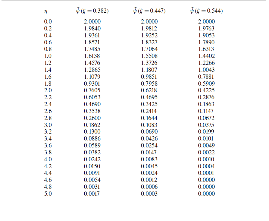
 ψ~(ξ,η)
 L=1=U
 ξ
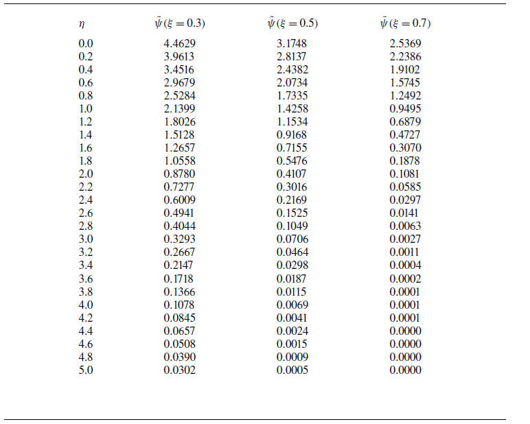
 ψ~(ξ,η)
 β=1/2
 L=1
 U=ξ1/3
 ξ=0.3,0.5,0.7


