


“A key characteristic of democracy,” Dahl (Reference Dahl1971, 1) noted, is the “responsiveness of the government to the preferences of its citizens.” Two mechanisms play central roles in promoting responsiveness, thereby fostering congruence between the preferences of voters and the policy positions of candidates. Voters in a democracy can select candidates that represent their views, and candidates can compete for votes by strategically taking positions that appeal to the electorate. Both mechanisms are important; each depends on the criteria voters use to judge politicians on the issues.
A lively debate has focused on three theories about how voters judge the policy stances of candidates. The first, proximity theory, assumes that citizens prefer candidates whose positions are closest to their own. For example, a voter who favors a 5% increase in government spending on health care will be happiest with a candidate who advocates the same level of spending. The more a candidate's position diverges from the voter's, the less satisfied the voter will feel. The presumed positive relationship between proximity and satisfaction, or utility, underlies the dominant framework political scientists have used in models of voting and electoral competition for more than half a century (Downs Reference Downs1957; see Grofman Reference Grofman2004 for a review of this voluminous literature).
The second theory, discounting, posits that candidates cannot fully deliver on their promises. Believing this, voters “discount” campaign pledges and judge each candidate based on the policies they expect the government to adopt if the candidate wins office (e.g., Adams, Bishin, and Dow Reference Adams, Bishin and Dow2004; Adams, Merrill, and Grofman Reference Adams, Merrill and Grofman2005; Fiorina Reference Fiorina1992; Grofman Reference Grofman1985; Kedar Reference Kedar2005). Unlike proximity voters, discounters do not necessarily prefer candidates whose stated positions match their own. Discounters may favor candidates unlike themselves, if such candidates stand the best chance of producing the most desirable policy outcomes.
In a seminal contribution to discounting theory, Grofman (Reference Grofman1985) emphasized the role of the status quo (existing government policy) in shaping expectations about what candidates can realistically achieve. According to Grofman, voters expect candidates to produce policies that fall somewhere between the status quo and the candidate's announced platform. Consider, once again, a voter who favors a 5% rise in government spending. Believing that elected officials typically move policy only part of the distance that they advocate, the voter might seek a candidate who proposes an increase of greater than 5%, rather than a candidate who advocates an increase of exactly 5%.
Directional theory, the third leading logic of issue voting, says that voters perceive political issues as two sided and want candidates who take their side or “direction” (Rabinowitz and Macdonald Reference Rabinowitz and Macdonald1989). Directional theory offers two related hypotheses. First, citizens prefer candidates on their own side of an issue over candidates on the opposite side. Second, given a choice between candidates on their side, voters support the most intense candidate because they regard intense candidates as more reliable and more committed to their cause. Directional theorists qualify this hypothesis, however, by noting that voters sometimes penalize extremely intense candidates for being beyond the “region of acceptability.”
These directional hypotheses potentially clash with other issue voting theories. Suppose, for example, that a voter takes a side but does not feel strongly about it. A directionalist would seek a highly intense proponent of their side. A proximilist, in contrast, would choose the closest candidate, even if that candidate were on the opposite side.Footnote 1
The relative frequency with which voters employ proximity, discounting, and directional criteria affects the selection mechanism at the heart of democracy. Scholars, political pundits, campaign professionals, and interested citizens often discuss whether candidates are taking winning or losing positions, whether candidates are advocating policies with enough intensity to impress voters, and the like. Such analyses rest on assumptions—usually implicit and untested—about how the policy pronouncements of candidates affect the choices of voters. Likewise, claims about the effects of political context rely on controversial assumptions about voters' decision rules. Changes in the status quo, for example, will have no electoral impact if voters are proximilists or directionalists but could shift the electoral tide if voters discount. To appreciate how issues get translated into votes, we must know what rules voters have in mind.
The mix of proximity, discounting, and directional voting should also affect candidate strategies. If voters follow a pure proximity rule, the optimal strategy for candidates is to locate at the ideal point of the median voter. If voters instead hew to a discounting criterion, candidates will prove most successful when they take positions on the side of the median voter opposite from the status quo. Finally, if voters make decisions consistent with directional theory, candidates will be most successful with policy stances near one extreme of the issue space. Of course, strategies also depend on nonissue considerations, which may lead candidates to deviate from these theoretically ideal locations. Nevertheless, the relative prevalence of each issue voting criterion in the electorate should guide candidates when running for office and constrain them while holding power.
More than 50 articles in peer-reviewed political science journals have attempted to adjudicate among these theories, and empirical analyses have involved public opinion polls from more than 20 countries around the world.Footnote 2 Despite this prolific academic debate, progress in estimating the prevalence of these decision rules in electorates has been limited by widely recognized roadblocks (Adams, Bishin, and Dow Reference Adams, Bishin and Dow2004; Lewis and King Reference Lewis and King1999; Merrill Reference Merrill1995).
One obstacle to progress has been the endogeneous relationship between candidate positions and voter behavior. This two-way relationship, so central to democratic theory, makes issue voting difficult to study. Ironically, the more candidates converge on the electorally optimal position, the less variation we see in candidate policies, and thus the less we can learn about issue voting by studying how people respond to the (small) remaining differences in candidate policies.
Previous research has also been limited by problems of measurement. Voters choose candidates not only on the issues, but also on charisma, competence, trustworthiness, and other factors that are hard to quantify, making it difficult to isolate the issue criteria that voters use. The standard method of measuring the issue positions of candidates—asking citizens where they think candidates stand—only exacerbates the problem by creating spurious relationships: voters project favorable positions onto candidates they prefer on other grounds. In addition, research has been impeded by the failure of surveys to measure the location of the status quo, a central concept in discounting theory.
We contribute to existing theoretical and empirical analyses in two ways. First, we formally derive the complete set of conditions under which the theories lead to distinctive predictions about how people vote. Second, we systematically test all three theories by conducting experiments that are tailored to our formal derivations. The experiments, embedded in public opinion surveys, avoid problems of endogeneity and measurement that have impeded previous research. Our experiments also use a unique and efficient method of assigning treatments. By adapting the questionnaire to each respondent's own report of his or her policy preferences, we obtain precise estimates with less than one-tenth the sample size and cost of conventional experimental methods.
Using data from the experiments, we estimate the proportion of a nationally representative random sample of adults whose choices about federal health care policy are consistent with each of the three issue voting logics. We find that, on this important issue, voters typically employ proximity-based decision rules: they either choose the closest candidate or select the one who, in their estimation, will bring policy nearest to their ideal point. More precisely, 57.7% of respondents in our study behave as if they are following a pure proximity rule. Another significant proportion, 27.6%, discounts the announced positions of candidates by taking into account the location of the status quo when voting. Finally, 14.7% of respondents appear to follow directional logic.
These results establish an important benchmark: they show the distribution of decision rules under ideal conditions in which citizens know the views of candidates and vote entirely on the issues. To the extent that voters in actual elections are unsure about the policy preferences of candidates or are swayed by nonissue considerations, their behavior may diverge from the patterns in our experiments. Our findings can, therefore, be interpreted as showing how voters would behave in a purely issue-oriented campaign, or as isolating the issue voting component of a potentially more complicated utility function.
To deepen our findings and further validate our experimental method, we investigate how the characteristics of voters affect the decision rules they use. We find that discounting is more common, and directionalism less common, among ideological centrists and nonpartisans. This suggests that centrist voters, who often find themselves choosing between polarized candidates in contemporary American politics, make relatively sophisticated judgments that help align policy with their preferences (see also Fiorina Reference Fiorina1992). Moreover, the widespread practice of discounting by moderate voters should draw public policy toward the political center because when policy deviates from the center, these voters choose candidates who counterbalance the shift.
In summary, we find that the electorate is not single minded when it comes to policy voting. Some voters reward intense candidates, others reward candidates who take positions most like their own, and still others waver between these two extremes, depending on the current state of policy. Moreover, the attributes of individuals systematically predict which rule they employ. These findings offer a richer understanding of democratic elections and political competition.
OBSTACLES TO EMPIRICAL ANALYSIS
There are several widely recognized problems with using nonexperimental data and methods to test theories of issue voting. First, the positions of candidates are endogenous to the decision rules that voters employ. Rational candidates adopt positions that they regard as conducive to winning elections. The pressure to attract voters reduces variation in candidate locations, precluding researchers from studying the full range of candidate configurations that would be useful for testing theories of issue voting. Taken to an extreme, electoral pressures could drive candidates to converge, leaving voters to decide on nonissue criteria.
The standard procedure for measuring the issue positions of candidates—asking voters where they think candidates stand—introduces additional endogeneity. If voters project locations onto candidates they prefer for nonspatial reasons, researchers will overstate the importance of whatever issue voting rule the voter has in mind. Some authors confront this problem by assuming that each candidate has a single location, equal to the average of all voters' individual assessments. This, however, biases estimates of proximity voting downward by introducing measurement error in the distance voters perceive between themselves and candidates, and by reducing the sample variation in this distance (Lewis and King Reference Lewis and King1999; see also Merrill Reference Merrill1995).
A second shortcoming of existing studies is the lack of critical tests: configurations of candidates and voters in which the theories predict different choices. The most commonly used data, seven-point issue scales from the National Election Study (NES), provide almost no critical tests of directional versus proximity voting. With integer scales running from 1 to 7, we cannot test the hypothesis that voters choose candidates on their side of the issue over candidates who are closer but on the opposite side.Footnote 3 Moreover, only eight scenarios pit more intense candidates against less intense candidates that are closer to the voter. Six of these involve candidates at the most extreme points on the scale, arguably beyond the region of acceptability. The only two uncontroversial tests arise when respondents at 5 face candidates at 5 (favored by proximity theory) and 6 (favored by directional theory), and the mirror image in which respondents at 3 face candidates at 2 and 3. Thus, of the 196 permutations of individual and candidate positions on a seven-point scale, only two (approximately 1%) provide strong tests of directional versus proximity theory. In practice, the proportion of critical tests is even smaller because voters often perceive candidates as taking competing sides of an issue, and therefore being on opposite sides of the neutral point.
Of course, even when voters and candidates are arrayed such that all three theories favor the same candidate, the mix of voting rules is crucial for strategy and selection in a democracy. The electorally optimal position for candidates depends on the frequency of each rule, even though the resulting configuration of candidates may provide few opportunities for using individual-level survey data to determine which rules voters employ. Notwithstanding the paucity of critical tests in existing polls, the mix of voting rules affects how sensitive candidates are to changes in voter positions, how sensitive the electorate is to changes in candidate positions, how movements in the status quo shape elections, and the kinds of policies a democracy produces.
A third roadblock to inference is multidimensionality. In standard surveys such as the NES, respondents report an overall feeling score or vote choice for each candidate, rather than saying which candidate they prefer on each policy issue. Without strong assumptions about the weight respondents place on each issue in the survey, it is difficult to infer what decision rule they are using. Behavior that appears consistent with one voting rule could, in many contexts, be made consistent with other rules by changing the presumed importance of each dimension. Moreover, existing data offer little opportunity to discover whether voters apply different decision rules to different issues, and estimates about the “average” decision rule necessarily depend on the set of items in the survey.
A fourth obstacle to empirical analysis is the presence of nonissue considerations. In actual elections, voters weigh not only the policy platforms of candidates but also their charisma, competence, trustworthiness, and other intangibles. These extra considerations make it difficult to isolate the issue criteria that voters use. The problem of identification is particularly serious when nonspatial considerations correlate with candidate locations and are difficult to hold constant in statistical analyses. Recognizing these problems, Adams, Bishin, and Dow (Reference Adams, Bishin and Dow2004, 357) concluded that with existing data, “no crucial test distinguishing the models is possible on the basis of voting behavior in a single election.”
Finally, standard data sets typically do not contain the quantities necessary to distinguish discounting from the leading alternatives. The problem arises either because surveys imply that the neutral point is also the status quo (e.g., decrease taxes, keep taxes the same, increase taxes), or because they fail to ask about the location of the status quo. Merrill and Grofman (Reference Merrill and Grofman1997, 45), for example, could not test discounting vis-à-vis the alternatives because they “did not have a good operationalization of . . . the status quo point.” Likewise, Adams, Bishin, and Dow (Reference Calvert2004, 351) were “unable to distinguish between the directional and discounting models,” and therefore could “make no claims about the individual-level decision-making” that gave rise to their results. On occasion, researchers have asked what survey respondents expect candidates to deliver (Lacy and Paolino Reference Lacy and Paolino1998) or have exploited variation in political institutions that affect the ability of candidates to shape policy (Kedar Reference Kedar2005). These valuable studies have found support for discounting theory but have not estimated the prevalence of all three voting rules in the electorate.
In summary, previous research has been hampered by problems of endogeneity, the paucity of critical tests, the curse of high dimensionality, the presence of nonissue considerations, and inadequate measures of the status quo. As Lewis and King (Reference Lewis and King1999, 31) noted, “until survey researchers or experimentalists produce better measurement devices, or political methodologists generate better methodological approaches, the impasse will remain.” In the next section, we offer a theoretical and empirical way forward.Footnote 4
DERIVATION OF CRITICAL TESTS
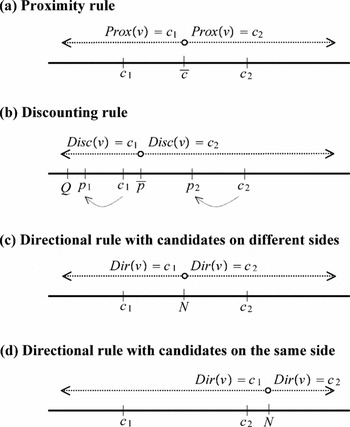
We now derive the conditions under which the three decision rules lead to distinct voting patterns. Consider a one-dimensional policy space: a number line that increases in value from left to right. The voter, whose position is denoted by v, faces a choice between candidates c 1 and c 2, with c 1 to the left of c 2. We use the functions Prox(v), Disc(v), and Dir(v) to indicate which candidate—c 1 or c 2—the voter at v would prefer if he or she were a proximilist, a discounter, or a directionalist.
Figure 1(a) displays how voters would behave if they were following the proximity rule. Recall that proximity voters prefer closer candidates to more distant ones. To express this idea formally, define the candidate mean, c =(c 1+c 2)/2, as the midpoint between the two candidates. Voters to the left of c are closer to c 1 than to c 2, and therefore prefer c 1 on proximity grounds. Voters to the right of c, however, are closer to c 2, making that candidate their proximity favorite. Finally, voters who stand exactly on c are equidistant between the candidates, and therefore have no preference for one over the other.
Proximity, Discounting, and Directional Rules

We use opposing arrows to summarize these predictions. Proximity voters who stand in the range covered by the left-pointing arrow, labeled Prox(v)=c 1, prefer c 1. Likewise, proximity voters with ideal points in the range covered by the right-pointing arrow, labeled Prox(v)=c 2, prefer c 2. The open circle above c means that, when a voter is equidistant between the candidates, proximity theory makes no prediction.
In the version of discounting theory that we examine, the policy that results from electing a candidate is a weighted average of the candidate's position and the status quo. Formally, p 1=αQ+(1−α)c 1 and p 2=αQ+(1−α)c 2, where Q is the location of the status quo and α ∈ (0,1) is the weight discounters assign to it. Let p =(p 1+p 2)/2 represent the midpoint between the policy outcomes that would result from choosing candidates 1 and 2, respectively. Voters to the left of p are closer to p 1 (the policy outcome associated with candidate c 1) than to p 2 (the policy outcome associated with candidate c 2), and would therefore favor c 1 under a discounting rule. Voters to the right of p would favor c 2, and voters at p would be indifferent between the two candidates.
Figure 1(b) illustrates these predictions for a scenario in which the status quo is to the left of the candidates. In such a configuration, the status quo pulls p 1 to the left of c 1 and pulls p 2 to the left of c 2, as indicated by the curved arrows below the number line. The straight arrows above the number line show how voters in different locations would behave if they were applying the discounting rule. Discounters in the region covered by the left-pointing arrow labeled Disc(v)=c 1 would opt for c 1, whereas discounters in the region spanned by the right-pointing arrow labeled Disc(v)=c 2 would choose c 2.
The location of the status quo is crucial to expectations about p 1 and p 2, and therefore to the choices of discounters. Had the status quo in our example been between the candidates, it would have played a moderating role by moving p 1 to the right of c 1 and moving p 2 to the left of c 2. If the status quo had been on the far right, in contrast, it would have tugged both policy outcomes to the right of the candidates' announced positions, thereby shifting p to the right and expanding the set of discounters who would have chosen c 1.
Directional theory emphasizes how candidates and voters are arrayed with respect to the neutral point, N, which may differ from the location of the status quo. When candidates are on opposite sides of the neutral point, as in Figure 1(c), directional voters prefer the candidate who advocates their side. Rabinowitz and Macdonald (Reference Rabinowitz and Macdonald1989) formalized this intuition by stipulating that each voter favors the candidate whose product (v−N)(c−N) is largest. If a voter takes the left side of the issue, then (v−N)(c 1−N) > (v−N)(c 2−N), and therefore c 1 is the better choice. If a voter takes the right side of the issue, the inequality reverses, and directional theory favors c 2. Neutral voters, who stand exactly on N, have no directional basis for choosing one candidate over the other. The opposing arrows mark the regions in which directional voters would prefer one of the candidates.
What happens when both candidates take the same side of an issue? Directional voters on that side prefer the more intense candidate, whereas directional voters on the opposite side prefer the less intense candidate. We illustrate this pattern in Figure 1(d), where both candidates endorse the left side of the issue. Applying the directional criterion, voters to the left of N would have (v−N)(c 1−N) > (v−N)(c 2−N) and choose c 1. Voters to the right of N, however, would have the reverse inequality and select c 2.
Having introduced our notation, we offer two propositions, which are proven in Appendix A.
Proposition 1. Proximity and discounting theories make distinct predictions if and only if the voter is between the status quo and the midpoint of the two candidates, and the discounter places a sufficiently high weight on the status quo. In symbols, let α* = (v − c)/(Q−c. Then Prox(v) ≠ Disc(v) iff α > α* and either Q < v < cor its reflection, c < v < Q.
Proposition 2. Proximity and directional theories make distinct predictions if and only if the voter is between the neutral point and the midpoint of the two candidates. In symbols, Prox(v) ≠ Dir(v) iff either N < v < cor c < v < N.
Proposition 1 distinguishes proximity from discounting theory. According to proximity theory, voters to the left of c prefer c 1, whereas voters to the right of c prefer c 2. The policy midpoint p plays an analogous role in discounting theory: voters to the left of p support c 1, but voters to the right of p support c 2. Consequently, the proximity and discounting rules imply different voting behavior only when the voter is between c and p. Proposition 1 establishes the necessary and sufficient conditions for “sandwiching” the voter between c and p. A key element in Proposition 1 is the weight of the status quo. If the voter placed no weight on the status quo, then p would coincide with c and the theories would make identical predictions. As the weight of the status quo increases, p shifts away from c in the direction of Q.Footnote 5 The value α* marks the transition point at which p crosses to the opposite side of v, causing discounters and proximilists to part ways.
As Proposition 2 shows, proximity and directional theories diverge under a different sandwich condition, in which the voter stands between c and N. Consider, for example, the configuration in which c < v < N. A directional voter would prefer c 1, the more intense candidate on the voter's side, whereas a proximity voter would prefer c 2, who is closer to the voter's ideal point.
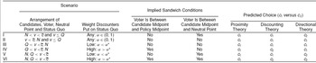
From these two propositions, we derive predictions for all possible arrangements of candidates, voters, the neutral point, and the status quo, for all possible weights that discounters could assign to current policy (see Appendix A for proofs). Table 1 lists the six key scenarios.Footnote 6 For each scenario, we give the implied sandwich conditions and indicate the choices a proximilist, a discounter, and a directionalist would make. Each scenario has an unlisted reflection—reversing the arrangement of candidates, the voter, the neutral point, and the status quo—that would lead to the opposite voting behavior. For example, the first row shows that with arrangement N < v < c and v ≤ Q, proximilists and discounters would prefer c 1, whereas directionalists would prefer c 2. In the mirror image arrangement, c < v < N and Q ≤ v, proximilists and discounters would favor c 2, but directionalists would incline toward c 1.
Predicted Choices in Six Scenarios

Note: α* =(v−c)/(Q−c).
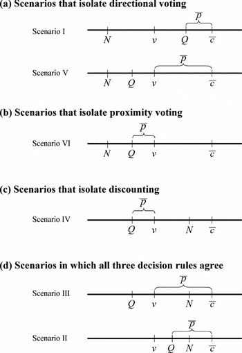
Figure 2 illustrates our predictions. Each panel in Figure 2 can be interpreted in light of our sandwich conditions: whether the voter is sandwiched between p and c (such that proximity and discounting theories disagree), and whether the voter is sandwiched between N and c (such that proximity and directional theories disagree). To isolate directional voting, for example, one must find scenarios in which the second sandwich condition holds but the first one does not. Figure 2(a) shows examples of the two scenarios that achieve this effect. To isolate proximity voting, both sandwich conditions must hold, as in Figure 2(b). To isolate discounting, the first sandwich condition must be true while the second must be false, as in Figure 2(c). Finally, when neither sandwich condition holds, all three decision rules agree, per Figure 2(d).
Scenarios That Isolate Each Decision Rule

EXPERIMENTAL DESIGN
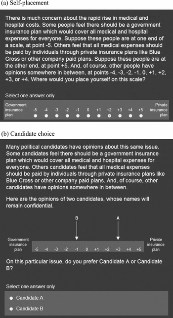
We designed an experiment that placed voters in the various scenarios and recorded the choices they made. The experiment, administered to a representative sample of U.S. adults over the Internet, began by measuring respondents' views about federal health care policy (Figure 3(a)). We chose health care because it is central to national policy debates,Footnote 7 is used to illustrate the differences between directional and proximity theories (e.g., Rabinowitz and Macdonald Reference Rabinowitz and Macdonald1989, 97), and does not require the status quo to be located at the neutral point.
Measuring the Voter's Position and Preferences About Candidates

The question format in Figure 3(a) was especially suitable for testing all three theories. Following the NES, we labeled only the end points of the scale. Assigning verbal labels to every point might have reduced ambiguity and increased reliability (Krosnick Reference Krosnick1999), but Rabinowitz and Macdonald (Reference Rabinowitz and Macdonald1989, 95) argued that labeling only the end points is best for comparing the theories. Such a scale not only “corresponds very nicely to the requirements of the traditional spatial model,” but also “permits directional thinking. Respondents thinking in directional terms would have little difficulty responding to this question. They would simply choose their preferred policy direction and how intensely they favored it.” In summary, NES-type scales “allow for either a directional or proximity interpretation, which is important for . . . empirical work” (Macdonald, Listhaug, and Rabinowitz Reference Macdonald, Listhaug and Rabinowitz1991, 1114).Footnote 8
We modified the NES format in two ways that improved our ability to draw inferences. First, we increased the number of scale points from seven to eleven to obtain a larger number of critical tests.Footnote 9 Second, we adopted different numeric labels. NES scales typically run from 1 to 7, leaving some ambiguity about the location of the neutral point. Our scale, in contrast, was centered on 0, a value respondents associate with neutrality (Schwarz et al. Reference Schwarz1991).
After recording the respondent's view, we displayed two candidates on the same scale and asked, based on the issue at hand, which candidate the respondent preferred (Figure 3(b)). To test proximity, discounting, and directional theories in their purest form, we described the candidates as “A” and “B.” Our design thereby avoided two obstacles described previously: the endogeneity of candidate locations and the presence of nonissue considerations.Footnote 10
Finally, we measured respondents' perceptions about the location of the status quo. “To the best of your knowledge,” we asked, “which point on the scale most closely represents the policy of the current government in Washington?” We placed this question last to avoid priming respondents to consider current policy when choosing between candidates. Our estimates of discounting may, therefore, be conservative, compared to what one would obtain by encouraging people to include the status quo in their voting calculus.
Our design was unique not only because it exogenously placed candidates on the scale and measured Q and vote choice, but also because it employed an efficient algorithm for locating candidates. Complete randomization of candidate positions would have been inefficient for two reasons. First, it would have generated many situations in which at least one theory failed to make a clear prediction. Second, full randomization would have resulted in an undesirably high proportion of ties, situations in which all three theories made the same prediction.
We gained efficiency by taking v into account when assigning candidates. In particular, we ensured that the theories made clear predictions (avoided situations in which voters would have been indifferent) by arraying the candidates such that c ≠ v, and by not treating respondents who located themselves at the neutral point. We also screened-out respondents at −5 and +5 because all three theories would have made the same prediction for those voters. A more efficient algorithm would have conditioned on Q as well, but asking about the status quo before displaying the candidates would have run the risk of priming bias.
To quantify the inefficiency of full randomization, we simulated the patterns that would have arisen if we had presented the respondents in our sample with a random array of candidates. Approximately 23% of the scenarios would have been indeterminate (at least one theory would not have made a prediction) and an additional 65% would have failed to discriminate (all three theories would have favored the same candidate). A further 9% would not have been informative, according to criteria discussed in the next section of the article. Only 3% of the cases would have provided critical tests necessary to estimate the frequency of proximilism, discounting, and directionalism in the electorate. Thus, simple random assignment—the standard approach in survey experiments—would have yielded remarkably little usable data. Informative cases were 13 times more common with our stratified randomization algorithm than with pure random assignment.Footnote 11
Thus, by letting formal theory guide the design of our experiment, we greatly increased the opportunity to estimate the relative importance of the three leading accounts of issue voting. Moreover, by assigning candidate locations that made optimal use of each voter's location, rather than distributing candidates completely at random, we conducted the experiment at far lower cost than otherwise would have been required.
STATISTICAL MODEL
From Table 1, which provided a basis for the experiment, we also developed estimators for the rates of proximity, discounting, and directional voting in the electorate. Suppose that all electors intend to follow one of the three canonical voting rules. Let πdir be the proportion of people who intend to follow a directional rule, let πdisc be the proportion who intend to discount, and let πprox=1 − πdir − πdisc represent the remaining share that intend to apply the proximity rule. To allow for the possibility of implementation error, assume that each voter makes the wrong choice—mistakenly selects a candidate not favored by that voter's decision rule—with probability e. (In Appendix B, we explore alternative assumptions about error.)
We can then model the probability that a randomly selected voter would choose candidate 2 (c 2). When confronted with scenario I, proximilists and discounters will mistakenly choose c 2 with probability e, whereas directionalists will correctly choose c 2 with probability 1−e. Consequently, the overall probability of choosing c 2 under scenario I can be decomposed as Pr(c 2|scenario I) ≡ πI = πproxe + πdisce + πdir(1−e), or πdir(1−2e) + e. Scenarios II and III imply a different pattern, in which all three types of voters will select c 2 only by mistake, such that Pr(c 2|scenario II) ≡ πII = e and Pr(c 2|scenario III) ≡ πIII = e. By similar logic, Pr(c 2|scenario IV) ≡ πIV = πproxe + πdisc(1−e) + πdire, or πdisc(1−2e) + e; Pr(c 2|scenario V) ≡ πV = πproxe + πdisce + πdir(1−e), or πdir(1−2e) + e; and Pr(c 2|scenario VI) ≡ πVI = πproxe + πdisc(1−e) + πdir(1−e), or (πdir + πdisc)(1−2e) + e.
To estimate the parameters in this model (πprox, πdisc, πdir, and e), we need a procedure for determining which scenario each of our survey respondents faced. It was easy to ascertain who confronted scenario I or scenario II. Those scenarios depended solely on the arrangement of the candidates, the voter, the neutral point, and the status quo, all of which we either measured or experimentally manipulated. It was more difficult to allocate the remaining respondents into scenarios III through VI. As is clear from Table 1, these scenarios depend on an unobserved quantity: the weight that each discounter, in his or her own mind, attaches to the status quo. Scenarios III and IV, for example, involve identical arrangements of the observed quantities (c, v, N, and Q). They nonetheless predict different behavior by discounters, depending on whether the weight they assign to the status quo is above or below the cutoff value α*. A discounter who gives the status quo low weight (α < α*) will choose the same candidate as a proximilist, but a discounter who gives the status quo high weight (α > α*) will select the other candidate. The remaining two scenarios in Table 1 (scenarios V and VI) are also isomorphic for all types except discounters, whose preferences depend on whether their private value for α is greater than α*.
We therefore devised a method for inferring whether discounters—to the extent they exist—had been assigned to scenario III versus IV or to scenario V versus VI. Our approach relies on the concept of an informative subset. Of the cases in which voters face Q < v < c, N (the arrangement shared by scenarios III and IV), we regard the portion in which α* < .1 as informative. Within that subset, any discounter who puts even slight weight on the status quo would satisfy the condition that α > α*, and would, therefore, perceive themselves as facing scenario IV instead of scenario III. Likewise, of the cases in which voters confront N, Q < v < c (the arrangement common to scenarios V and VI), we treat ones with α* < .1 as informative. In those cases, all but the most trivial discounters would see themselves in scenario VI, not scenario V.
Subsets in which α* ≥ .1 are not as informative because they make it impossible to distinguish reliably between discounters and proximity voters. In arrangements where α* is high, even discounters who place substantial weight on the status quo may fail to satisfy the condition that α > α*. In our experiment, they would make the same choices as similarly situated proximilists, even though they reached a decision after discounting the announced positions of the candidates. To estimate whether and to what extent discounters exist in the electorate, we must focus on the subset of cases in which we can actually detect them and discard the remainder.
This framework implies a set of error-adjusted estimators for the prevalence of directional, discounting, and proximity rules, where IV* denotes the informative subset of scenarios III and IV, and where VI* denotes the informative subset of scenarios V and VI.

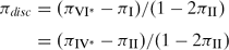

In our sample, there were no instances of scenario IV*, so Equation (2) simplified to πdisc = (πVI* − πI)/(1−2πII). By computing the proportion of respondents in scenarios I, II, and VI* who chose candidate c 2, and substituting the proportions into Equations (1) and (2) as values for πI, πII, and πVI*, one can estimate the rates of proximity, discounting, and directional voting while taking voter error into account.Footnote 12 We quantify the uncertainty associated with our estimates by taking bootstrap samples from the pruned data set that contains only scenarios I, II, and VI*.Footnote 13
ESTIMATED PREVALENCE OF THE DECISION RULES
The surveys discussed in this article were administered by Knowledge Networks, an Internet-based polling firm, with support from the National Science Foundation. By using random digit dialing to recruit participants and by providing Internet access to households, Knowledge Networks was able to administer our questionnaires to a nationally representative sample of U.S. adults.Footnote 14 The interviews took place between December 2005 and June 2006, and 3,315 people (72% of invitees) agreed to take the survey. We did not continue with respondents who located themselves at −5, 0, or +5 on the first item, the health care scale, because they would not have yielded critical tests. Of the remaining people, 1,564 completed our experimental protocol, yielding 1,045 informative cases.Footnote 15
Table 2 summarizes the behavior of respondents in each informative scenario. The table shows, for example, that 25.67% of the 261 respondents who faced scenario I chose candidate c 2 rather than c 1. The table also reports the decisions of citizens in scenarios II and VI*.Footnote 16 As noted previously, the sample contained no instances of the informative subset IV* because citizens who faced the arrangement shared by scenarios III and IV did not locate the status quo such that α* was less than .1.Footnote 17
Predicted versus Observed Choices

Note: When estimating the observed preference for c 2, we classified a case as scenario I if N < v < c and v ≤ Q; as scenario II if v < c, N and v ≤ Q; and as scenario VI* if N, Q < v < c and α* < .1. The sample contained no examples of scenario IV*, in which Q < v < c, N and α* < .1.
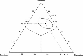
From the 1,045 cases in Table 2, we inferred the prevalence of proximilism, discounting, and directionalism in the population. Our estimates imply that about 57.7% of citizens use a proximity decision rule, 27.6% choose after discounting the announced positions of candidates, and the remaining 14.7% apply directional logic.Footnote 18 It bears repeating that these estimates already account for voter error. We assumed that each voter mistakenly chose the wrong candidate—chose c 1 when they preferred c 2, or vice versa—with probability e. (Our conclusions are robust to alternative assumptions about error, as shown in Appendix B.) We then calculated e as the rate at which citizens in scenario II chose c 2 and incorporated e into our estimates of the three voting rules.
Consider the case of directional voting. Had we ignored error, we would have classified 25.7% of voters as directionalists, because that share of citizens chose c 2 when presented with scenario I. However, we estimated an implementation error rate of about 15.5%. In our model, this means that around 15.5% of voters who intended to follow proximity or discounting rules in scenario I inadvertently selected the directional favorite. At the same time, around 15.5% of directionalists who encountered scenario I mistakenly opted for the proximity/discounting favorite. Equation (1) takes these countervailing errors into account. The error-corrected estimate of directional voting is, therefore, (πI − πII)/(1−2πII) = (0.2567-0.1552)/(1−2 × 0.1552) ≈ 14.7%.
Our estimates and associated measures of uncertainty are depicted in Figure 4. The figure, a ternary plot, is useful for displaying three estimates that must sum to 100 and are therefore interdependent. The height of any point in the plot (the perpendicular distance from the base to the top vertex) measures the frequency of proximity voting. If all voters were proximilists, we would place a point on the upper vertex. If only half were proximilists, the point would sit on a horizontal line parallel to the base and midway between the top and the bottom. And if proximilists were entirely absent from the sample, we would place a point somewhere on the triangle's base. Similarly, the rate of discounting is equal to the perpendicular distance from the left side of the triangle to the lower right vertex, with points on the left side implying no discounting and a dot on the lower right vertex implying that all voters are discounters. Finally, the rate of directional voting is given by the perpendicular distance from the right side of the triangle to the lower left vertex.
Estimated Prevalence of Voting Rules

The black dot in the triangle's interior represents our best estimate of the shares of the population that adhere to each voting rule. Dotted lines emanate from the point to the relevant numeric scales on each side. The line that runs parallel to the base and intersects the left side of the triangle shows that the dot is 57.7% of the distance from the base to the top, representing the share of proximilists in the population. Dotted lines that parallel the left and right sides of the triangle reflect the proportions of discounters and directionalists, respectively. The solid line around the dot is a 95% confidence region.Footnote 19
The closer a point is to a given vertex (with closeness measured perpendicular to the base), the more pervasive the decision rule associated with that vertex. The dashed lines that divide the triangle into three equal areas establish which voting rule is most common. The dot and its associated confidence region fall entirely within the upper region. Thus, a plurality of voters in our experiment behaved consistently with the proximity rule.
TESTING ADDITIONAL IMPLICATIONS OF THE THEORIES
To further validate our experimental method and test additional implications of the theories, we examined whether the distribution of proximity, discounting, and directional voting differs for subgroups of the population. Some authors have speculated that less sophisticated and less informed citizens are especially likely to employ a directional decision rule because it is less cognitively and informationally demanding. Empirical studies have found little support for this hypothesis, however (Merrill and Grofman Reference Merrill and Grofman1999, 79). Along similar lines, one might hypothesize that discounting, which requires an understanding of the policy-making process, increases with the sophistication of voters. We used educational attainment as a proxy for political knowledge and sophistication.
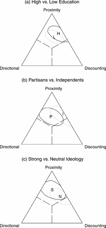
To assess the effect of education, we estimated our model separately for people with and without a college degree. Estimates for the two subgroups appear in Figure 5(a). Directional voting was about twice as common among the less educated respondents (18.6%) as among the more educated ones (8.5%). In contrast, we found little evidence of a connection between discounting and education. The college graduates in our sample practiced discounting only 3.3 percentage points more often than those without college degrees.
Estimates by Demographic Group

The political characteristics of respondents may also affect their incentives to use a discounting decision rule. Fiorina (Reference Fiorina1992), for example, hypothesized that when moderate citizens confront extreme politicians, they vote to put different branches of government under the control of rival camps that must compromise to produce policy. Others have found evidence that politically independent voters are especially likely to engage in this sort of calculus (Lacy and Paolino Reference Lacy and Paolino1998, 1181). Accordingly, we hypothesized that two groups—people without partisan affiliations and people with moderate political ideologies—would be more likely to engage in discounting behavior than more politically committed and extreme citizens.
To evaluate this hypothesis, we estimated our model separately for the most and least partisan thirds of our sample (strong partisans versus independents and leaners) and for the most and least ideological thirds of the sample (those at 1, 2, 6, or 7 versus those at 4 on the 7- point ideology scale). Figure 5(b) confirms that the three decision rules had different distributions among independents than among strong partisans. The estimated share of independents that discount (38.9%) was nearly twice as large as the share of strong partisans that discount (22.0%). More striking and less expected, directionalists were almost absent among political independents but comprised one-fourth of strong partisans. Similarly, Figure 5(c) shows that political moderates were nearly twice as likely as strong ideologues to employ a discounting decision rule (37.9% versus 18.6%). Thus, the political characteristics and commitments of voters affect patterns of issue voting.
THE POSSIBILITY OF MIXED MODELS
Our statistical model assumes that each voter follows one of the three canonical issue voting rules. An alternative perspective holds that all voters employ a common, mixed decision rule. Rabinowitz and Macdonald (Reference Rabinowitz and Macdonald1989, 110) raised the possibility that voters combine directional and proximity criteria, and Iversen (Reference Iversen1994) developed a theoretical justification for such a model. Merrill (Reference Merrill1995), too, offered a mixed directional-proximity model, which Merrill and Grofman (Reference Merrill and Grofman1999) extended by incorporating discounting to yield a “unified theory of voting.”
Although some authors have found support for mixed models, Merrill and Grofman (Reference Merrill and Grofman1999, 79) noted a problem of interpretation: “It is possible that some voters evaluate candidates according to the proximity model, whereas others use a directional measure. In other words, heterogeneity among voters is an alternative explanation to individual mixed utilities.” Unfortunately, neither standard surveys nor our experiments allow one to know definitively whether the voting population is composed of homogenous mixers, heterogeneous purists, or something in between.
Researchers may gain insight, however, by examining whether people in different demographic subgroups employ different rules. Merrill and Grofman (Reference Merrill and Grofman1999, 79) found little evidence that levels of directional voting vary with political sophistication and other demographic factors, and therefore concluded that people probably make compound utility calculations. “Still,” they noted, “it is possible that an alternative method of subgrouping would reveal heterogeneity for utility functions.”
Our experiments uncovered evidence that different subgroups judge the platforms of candidates in different ways. This conclusion was possible because our study, unlike previous ones, distinguished empirically among all three decision rules. More research is needed, but our findings support the hypothesis of voter heterogeneity—the claim that different voters employ different pure rules or different mixtures—rather than the hypothesis that all voters have homogeneous mixtures (for further evidence of heterogeneous decision criteria, see Rivers Reference Rivers1988).
If, however, one believes that voters mix directional, discounting, and proximity rules, our findings establish bounds on the shares of the population that include each element in their mix. Based on our data, at least 14.7% of citizens have a directional component to their utility function, and at least 27.6% consider the location of the status quo when choosing among candidates. It is more difficult to put lower bounds on the proportion of voters that assign at least some weight to pure proximity because the proximity-consistent choices in our sample could be due to discounters who place very low weight on the status quo. However, our data show that more than 85% of citizens have either a proximity or a discounting component in their issue voting calculus.
CONCLUSION
Our theoretical analyses identify, for the first time, the complete set of conditions under which the three most prominent theories of issue voting make distinctive predictions about how citizens vote. Our experimental approach uses these predictions to assess how people choose candidates on the issue of federal health care policy.
We find that proximity voting is about twice as common as discounting and four times as common as directional voting. These results establish a new benchmark for understanding how the policies of candidates affect the choices of voters. We isolated the policy component in the voter's calculus by focusing on a single issue, thereby avoiding assumptions about how voters weigh policies in multiple dimensions, and by stripping away nonissue considerations, thereby avoiding traditional measurement problems. We also provided respondents with specific information about candidates' stances, thus minimizing the potential for uncertainty to distort spatial judgments. Future research could go beyond our benchmark by examining voter behavior on different issues and in more complex settings. For example, directional voting may be more common on moral issues that some people characterize as dichotomous, while being less common on budget issues that offer a fine-grained array of alternatives.
The discovery that different voters use different decision rules has important implications that could be explored both theoretically and empirically in subsequent studies. Heterogeneous populations, in which large segments employ each rule, might stimulate different candidate strategies and electoral outcomes than homogenous populations. Morris and Rabinowitz (Reference Morris and Rabinowitz1997, 75), for example, developed a model in which some citizens are proximity voters and others apply directional criteria. They proved that “candidates trying to optimize support in this heterogeneous environment will generally adopt more extreme positions than those implied by proximity theory and more central positions than those implied by directional theory.” As a natural extension, one could model candidate behavior in the presence of discounters as well.
The heterogeneity we have uncovered may even help explain the polarization that persists in many democratic systems and is particularly prevalent in contemporary American politics. None of the basic theories, on its own, can account for the existing divergence in candidate positions. It is well known that proximity theory, in its simplest form, predicts that candidates will converge on the ideal point of the median voter. It is less appreciated that discounting and directional theories also predict candidate convergence, albeit often at an extreme rather than a centrist position.Footnote 20 In a mixed population, though, the winning move may be difficult for candidates to identify. Calvert (Reference Calvert1985) showed that candidates may diverge to some degree if they are partly motivated by policy and uncertain about how proximity voters will react to their positions. Being uncertain about the distribution of decision rules in the electorate could fuel more polarization, particularly if candidates cannot be sure whether pivotal voters would favor centrist or extremist candidates.
Our study also reinforces and extends an emerging body of research, which shows that many voters focus on the policies candidates will deliver, rather than the ones candidates espouse. Evidence of this phenomenon comes not only from Senate elections and presidential contests in the United States (Adams, Bishin, and Dow Reference Adams, Bishin and Dow2004; Lacy and Paolino Reference Lacy and Paolino1998), but also from other countries. In a study of parliamentary elections in Europe, for example, Kedar (Reference Kedar2005) found that voters recognize the institutional constraints on power and take those constraints into account when deciding who to support. We find a related form of sophisticated reasoning: many voters consider the location of the status quo when deciding which candidate to support. Together these studies, employing a wide range of methods and data, paint a consistent picture of electoral politics in which discount-minded voters play an important role.
Finally, our analyses show that the prevalence of each rule varies across politically relevant subgroups of the population. Voters in the center of the political spectrum—judged either by their self-professed ideology or by their failure to identify with either major political party—are twice as likely as more committed voters to take existing policy into account. Thus, politically moderate citizens appear quite attentive to the political environment. This finding, which may seem surprising, comports with the claim by Fiorina (Reference Fiorina1992) and others that moderates make relatively sophisticated electoral choices aimed at dividing power between extremists and forcing policy compromise. Ultimately, discounting by centrists will tend to moderate public policy by pulling it toward the center when it shifts too far in one direction or the other.
The methods and data in this article shed new light on the way voters judge the issue stances of candidates. By providing benchmark estimates for the three leading theories of issue voting, documenting heterogeneity in the American electorate, and exploring the demographic correlates of this heterogeneity, we advance a debate that is central to understanding how democracy works. At the same time, we provide a template for future studies. Using the formal derivations, statistical model, and experimental methods described here, researchers can now investigate the three leading theories of issue voting in a variety of contexts. Such research could provide a firmer basis for understanding how the policy preferences of citizens affect the selection and strategic behavior of elected officials.
APPENDIX A: PROOFS OF CRITICAL TEST CONDITIONS
Lemmas. The following lemmas deal with real numbers x 1 and x 2, with x 1 < x 2. Let x = x 1 + x 2)/2, the midpoint between x 1 and x 2.
Lemma 1. If v is to the left of x, then v is closer to x 1than to x 2. In symbols, if v < x, then (v−x 1)2 < (v−x 2)2. Proof: Let v < x. Then v < (x 1 + x 2)/2, or 2v < x 1 + x 2. Because x 1 < x 2, x 2−x 1 > 0. Thus, we can write 2v(x 2−x 1) < (x 1 + x 2)(x 2 − x 1). After some algebra, we find that x12 − 2vx 1 < x 22 − 2vx 2. Adding v 2 to both sides gives v 2 − 2vx 1 + x 12 < v 2 − 2vx 2 + x 22, or (v − x 1)2 < (v−x 2)2.
Lemma 2. If v is to the right of x, then v is closer to x 2than to x 1. In symbols, if x < v, then (v−x 2)2 < (v−x 1)2. The proof follows the same logic as Lemma 1.
Proposition 1. Define c = (c 1 + c 2)/2, the midpoint between c 1and c 2, and let α* = (v − c)/(Q − c. Then Prox(v) ≠ Disc(v) iff α > α* and either Q < v < cor its reflection, c < v < Q.
Proof. The proof proceeds in two steps. In Step 1, we show that Prox(v) ≠ Disc(v) iff either p < v < c or c < v < p, where p = (p 1 + p 2)/2. In Step 2, we show that these conditions are equivalent to the voter being between Q and c and assigning a weight in excess of α* to the status quo.
Step 1. Let p < v < c and assume, without loss of generality, that c 1 < c 2. With c, Lemma 1 implies that (v−c 1)2 < (v−c 2)2, and therefore Prox(v) = c 1. Moreover, because p < v, Lemma 2 implies that (v−p 2)2 < (v−p 1)2, which means that Disc(v) = c 2. Consequently, Prox(v) ≠ Disc(v). A similar logic applies to the mirror image: if c < v < p, then Prox(v) = c 2 ≠ Disc(v) = c 1. We have, therefore, established sufficient conditions for distinguishing the proximity favorite from the discounting favorite.
We now show that those conditions are necessary. Consider the four scenarios in which the voter is not strictly between p and c. In the first arrangement, v < c, p. By Lemma 1, (v−c 1)2 < (v−c 2)2 and (v−p 1)2 < (v−p 2)2, which mean that Prox(v) = Disc(v) = c 1. The second scenario is the mirror image, in which c, p < v. By a similar proof that invokes Lemma 2, Prox(v) = Disc(v) = c 2. The remaining two scenarios are degenerate cases. If v = c, the voter is equidistant between c 1 and c 2, so neither candidate is the proximity favorite. Finally, if v = p, the voter is equidistant between the policy outcomes associated with c 1 and c 2, so neither candidate is the discounting favorite.
Step 2. Let p < v < c. This implies a value of α such that (α Q + (1−α)c 1 + α Q + (1−α)c 2)/2 < v. After some algebra, α (Q−c) < v−c, a relationship we will examine for three mutually exclusive and exhaustive scenarios. In the first scenario, Q < c, so α > (v − c)/(Q− c) ≡ α*. Moreover, because α must be less than 1, we can write (v−c)/(Q−c) < 1, which simplifies to Q < v. In the second scenario, Q = c, which would mean that 0 < v−c, or c < v. This scenario, therefore, is ruled out by the assumption that v < c. In the third scenario, c < Q, which would imply α < (v− c)/(Q−c). However, because α must be greater than 0, we would then have 0 < (v−c)/(Q−c) or c < v, a violation of our assumption that v < c. Thus, condition p < c holds only in the first scenario and can be restated as the intersection of Q < v < c and α > α*. By a similar proof, the condition c < p can be reexpressed as the intersection of c < v < Q and α > α*.
Proposition 2. Prox(v) ≠ Dir(v) iff either N < v < cor c < v < N. ***
Proof. Let N < v < c and again assume, with out loss of generality, that c 1 < c 2. Then by Lemma 1, (v−c 1)2 < (v−c 2)2, and therefore Prox(v) = c 1. Moreover, because c 1 < c 2, (c 1−N) < (c 2−N), and because N < v, (v−N) > 0. Thus, (c 1−N)(v−N) < (c 2−N)(v−N), making Dir(v) = c 2. Consequently, Prox(v) ≠ Dir(v). A similar logic applies to the mirror image: if c < v < N, then Prox(v) = c 2 ≠ Dir(v) = c 1. We have, therefore, established sufficient conditions for distinguishing the proximity favorite from the directional favorite.
We now show that those conditions are necessary. Consider the four scenarios under which the voter is not strictly between N and c. In the first scenario, v < c, N. By Lemma 1, (v−c 1)2 < (v−c 2)2, which makes Prox(v) = c 1. Moreover, because c 1 < < c 2, (c 1−N) < (c 2−N), and because v < N, (v−N) < 0. Thus, we can write (c 2−N)(v−N) < (c 1−N)(v−N), which means Dir(v) = c 1, the same candidate favored by proximity theory. The second scenario is the reflection, c, N < v. By a similar proof that involves Lemma 2, Prox(v)= Dir(v) = c 2. In the third scenario, v = c, so neither candidate is the proximity favorite. Finally, if v = N, the product (c−N)(v−N) is the same for both c 1 and c 2, and therefore neither candidate is the directional favorite. ***
Corollary 1. Prox(v) ≠ (Disc(v) = Dir(v)) iff N., Q <v < cor its reflection and α > α*. Proof: Intersect the conditions under which Prox(v) ≠ Disc(v) with the conditions under which Prox(v) ≠ Dir(v).
Corollary 2. Disc(v) ≠ (Prox(v) = Dir(v)) iff Q < v c, N or its reflection and α > α*. Proof: Intersect the conditions under which Disc(v) ≠ Prox(v) with the conditions under which Prox(v)=Dir(v).
Corollary 3. Dir(v) ≠ (Prox(v)=Disc(v)) iff either (1) N < v < c and v ≤ Q or the reflection of these conditions, or (2) N, Q < v < cor its reflection and α < α*. Proof: Intersect the conditions under which Dir(v) ≠ Prox(v) with the conditions under which Prox(v) = Disc(v).
Corollary 4. Prox(v) = Disc(v)=Dir(v) iff either (1) c, N < v and Q ≤ v or the reflection of these two conditions, or (2) c, N < v < Q or its reflection and α < α*. Proof: Intersect the conditions under which Prox(v) = Disc(v) with the conditions under which Prox(v) = Dir(v).
APPENDIX B: ALTERNATIVE ASSUMPTIONS ABOUT ERROR
Equations (1) through (3) assume that all voters try to follow one of the three voting rules but choose the wrong candidate with probability e. Alternatively, one could assume that voters facing close calls err at a higher rate than voters facing easy choices. Close calls occur when a proximity voter is near c, a discount-minded voter is near p, or a directionalist is near N and/or faces candidates who take the same side with similar intensity. With the data at hand, we cannot fully identify close calls because p is a function of each voter's private beliefs about α. By introducing extra assumptions, though, we can derive and estimate a model in which the error rate varies across individuals, depending on the scenarios they face.
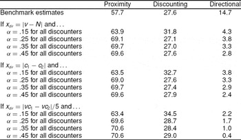
Suppose that, in addition to a baseline error rate e, voters make mistakes at an extra rate f(x), where x measures the ease or difficulty of their choice. For proximity voters, let x prox be the voter's absolute distance to the candidate midpoint, |v−c|, such that lower values represent closer calls. For discounters, assume a value for α, and then let x disc be the voter's absolute distance to the policy midpoint, |v−p|. For directionalists, we explore three possible values of x dir: the voter's absolute distance to the neutral point, |v−N|; the absolute difference between the views of the two candidates, |c 1−c 2|; and the absolute difference in directional utilities, |vc 1−vc 2|, which we divide by 5 to make its range comparable to the ranges of the other measures of x.
Assume the probability of error is approximately .5 when the voter faces an extremely close call (when x is close to zero) and declines exponentially toward zero as x increases. To capture this idea, let f(x) = 0.5 exp(gx), where g < 0 governs the rate of decline. Then Pr(c 2| scenario I) ≡ πI = πprox(f(x prox) + e) + πdisc(f(x disc) + e) + πdir(1−f(x dir)−e); Pr(c 2| scenario II) ≡ πII = πproxf(x prox) + πdiscf(x disc) + πdirf(x dir) + e; and Pr(c 2| scenario VI*) ≡ πVI* = πprox(f(x prox) + e) + πdisc(1−f(x disc) − e) + πdir(1−f(x dir)−e). By substituting these expressions into a binomial likelihood and maximizing it with respect to πprox, πdisc, πdir, e, and g, we can estimate the prevalence of each voting rule while accounting for errors related to close calls.
Even with these additional assumptions, our main conclusions continue to hold (Table 3). The estimated prevalence of discounting was 27% to 35% across various measures of close calls, compared with around 28% in our benchmark model. Directional voting appeared somewhat less common, and proximity voting somewhat more common, in this alternative model than in our benchmark one. The estimates shifted slightly because our sample contained more close calls (as we defined them) by proximity criteria than by directional criteria.
Sensitivity Analyses: Alternative Assumptions About Error

Note: Benchmark estimates assume that all voters make implementation errorsat a common rate, e. All other scenarios allow error rates to vary by individual. Across all specifications, the maximum-likelihood estimate of g in the individual-specific error component f(x)=.5 exp(gx) ranged from −2.2 to −2.4.
We conclude by considering one final approach to error. What if some people choose completely at random, whereas others follow the canonical rules without error? To explore this possibility, let 2e represent the proportion of random choosers in the population. This implies πI = πdir+e; πII = e; and πVI* = πdisc + πdir + e. Based on this model, random choosers make up 31% of our sample. The presence of random choosers does not change the relative frequency of other rules, however. Proximilism is still twice as prevalent as discounting and four times as widespread as directionalism: the estimated rates are 40%, 19%, and 10%, respectively. Overall, the analyses reported here reinforce our key findings: all three rules are evident, but proximity voting outstrips discounting, which in turn outstrips directional voting.




Comments
No Comments have been published for this article.