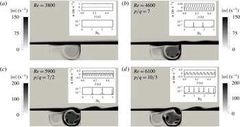
1 Introduction
The self-excited resonances appearing in spatially developing flows enable us to explain the sharp selection of definite wavenumbers and frequencies observed in experiments. A paradigmatic example of hydrodynamic resonance is the wake flow behind bluff bodies at low Reynolds number, in which oscillations occur with a distinct frequency and wavenumber (Pierrehumbert Reference Pierrehumbert1984; Koch Reference Koch1985). The nature of this resonance is related to the stability characteristics of wake flows, which presents the possibility of amplifying perturbations in the region upstream of the source. In shear flows like mixing layers or boundary layers, perturbations are swept away from the source, and unless a coherent perturbation is imposed, the measured spectra remain broadband. However, when a feedback mechanism is possible, these flows may also exhibit discrete frequency spectra. The feedback may take place as a consequence of the downstream reflection, and upstream propagation, of some of the waves of the perturbing wavepacket, which then reach again the region where the perturbation originated. The reflection may occur either in a turning point (Kulikowskii & Shikina Reference Kulikowskii and Shikina1996), or in a fixed boundary. The latter case results in impinging flows on solid boundaries, extensively studied as reported in Rockwell & Naudascher (Reference Rockwell and Naudascher1978), Knisely & Rockwell (Reference Knisely and Rockwell1982), Ziada & Rockwell (Reference Ziada and Rockwell1982). In particular, in open cavity flows, the impingement of the unstable shear layer onto the downstream edge of the cavity produces a global feedback, responsible for self-sustained oscillations of the flow beyond a critical value of both Reynolds number and cavity length – see for instance Rockwell & Naudascher (Reference Rockwell and Naudascher1978) for an early review on the topic. Those self-sustained oscillations are known to be the source of noise in many applications (e.g. fast train, aircraft land gear bay) or harmonious sound in wind instruments (e.g. in a saxophone). In compressible flows, this phenomenon is commonly linked to the acoustic feedback mechanism first introduced by Rossiter (Reference Rossiter1964). Incompressible open cavity flows still remain an active field of research including Rowley, Colonius & Basuz (Reference Rowley, Colonius and Basuz2002), Lusseyran, Pastur & Letellier (Reference Lusseyran, Pastur and Letellier2008), Basley et al. (Reference Basley, Pastur, Lusseyran, Faure and Delprat2011), to cite only a few of them, as the feedback mechanism through far-field acoustic waves travelling upstream loses importance due to other pure hydrodynamics mechanisms. A recent linear instability analysis by Tuerke et al. (Reference Tuerke, Sciamarella, Pastur, Lusseyran and Artana2015), considering reflection of hydrodynamic waves at the wall of the cavity, was able to describe the origin of the non-harmonic quantization of frequencies reported in different experiments. This analysis, however, is unable to distinguish, among the set of possible frequencies, which ones are selected by the flow. This limitation indicates that other hydrodynamic mechanisms, associated with the confinement of the flow, have to be taken into account. In an open cavity, a recirculating zone is established with complex intracavity vorticity patterns formed by vortex structures of different sizes that are expected to participate in the feedback mechanism (Basley et al. Reference Basley, Pastur, Delprat and Lusseyran2013). The interaction of these structures with the onset of the shear instability is nevertheless delayed by the time lag necessary for their transport from the impinging region to the upstream flow. This nonlinear delayed action on the upstream shear-layer instability has been modelled in confined jets with a formalism referred to as the nonlinear delayed saturation model (Villermaux & Hopfinger Reference Villermaux and Hopfinger1994). Inspired by this work, the dynamics of each cavity can be conceived in terms of nonlinear oscillators. The small structures, present in the recirculation region, produce discontinuous and delayed feedback, giving rise to nonlinear dynamical features, such as quasi-periodic oscillations, phase-locked oscillations or even chaotic dynamics (Villermaux & Hopfinger Reference Villermaux and Hopfinger1994).
When two identical self-oscillating systems are brought together, the dynamics can be expected to be enriched with additional couplings and interactions. Some of these examples are side-by-side cylinder flows (Zhou, Zhang & Yiu Reference Zhou, Zhang and Yiu2002; Kang Reference Kang2003; Landel, Caulfield & Woods Reference Landel, Caulfield and Woods2012) or two mirrored backward facing steps (Durst, Melling & Whitelaw Reference Durst, Melling and Whitelaw1974; Fearn, Mullin & Cliffe Reference Fearn, Mullin and Cliffe1990). At very close distances the two systems lose identity and behave as a new system. When two open cavities face each other, a so-called double cavity configuration is created, and one may presume the appearance of dynamical couplings of the two shear layers originating from each wall of the inlet channel. Research related to different industrial and bio-mechanical applications is concerned with these flows: the sudden expansion and contraction in pipe and channel flows (Drikakis Reference Drikakis1997; Mizushima & Shiotani Reference Mizushima and Shiotani2001; Mullin, Shipton & Tavener Reference Mullin, Shipton and Tavener2003), the exit of confined jets (Maurel et al. Reference Maurel, Ern, Zielinska and Wesfreid1996; Righolt et al. Reference Righolt, Kenjereš, Kalter, Tummers and Kleijn2015) and the laryngeal ventricle or Morgagni’s sinus in the human phonatory system (Agarwal, Scherer & Hollien Reference Agarwal, Scherer and Hollien2003; Chisari, Artana & Sciamarella Reference Chisari, Artana and Sciamarella2011) are just a few examples, among others, in engineering applications and nature, in which the understanding of the flow physics of double cavity dynamics is of importance.
Maurel et al. (Reference Maurel, Ern, Zielinska and Wesfreid1996) considered a confined planar jet issuing into a large cavity, a geometry that is similar to the double cavity. The experiments were performed with a ratio between the inlet channel height (
 $D$
) and the cavity depth (
 $H$
) equal to
 $1/12$
, and the varied geometrical parameter was the length
 $L$
of the cavity. The authors found a stable flow regime with no oscillations, a regime with self-sustained oscillations and a regime with turbulent-free jet characteristics. In the self-sustained oscillation regime, the authors observed that the flow was mainly two-dimensional, and proposed a subdivision of this regime into a sinuous mode with large scale wavelengths and a varicose mode with much shorter wavelengths. The case with constant
 $L/H$
and varying
 $D$
was not investigated by Maurel et al. (Reference Maurel, Ern, Zielinska and Wesfreid1996). By sufficiently increasing the ratio
 $D/H$
, the two shear layers extend but do not merge along the cavity length
 $L$
. The confined jet behaviour vanishes and double cavity flow arises. For sufficiently large
 $D$
the single cavity flow behaviour is expected to be retrieved. Mizushima & Shiotani (Reference Mizushima and Shiotani2001), Mullin et al. (Reference Mullin, Shipton and Tavener2003) investigated the symmetry, stability and bifurcation properties of double cavity flow as the Reynolds number is varied. For some cases the Reynolds numbers is comparable to the present work, however
 $L/H$
is much greater, leading to asymmetric flow configurations.
The aim of this paper is to understand the nonlinear frequency selection mechanisms in double cavity flow, focusing on the role of the backflow structures of the recirculation region, observed experimentally for single cavity flow by Basley et al. (Reference Basley, Pastur, Lusseyran, Faure and Delprat2011). We address the question of how this feedback mechanism develops as the Reynolds number is increased and whether or not a general route to chaos can be observed. Conceptually, this approach is similar to Johnson & Patel (Reference Johnson and Patel1999) and Tomboulides & Orszag (Reference Tomboulides and Orszag2000), who characterized the flow regimes around a sphere in the transition to turbulence.
The present analysis is based on results issued from two-dimensional numerical simulations. The numerical study we propose has the advantage of allowing a detailed parametric study, in a reasonable simulation time, with a greater control of variables than in physical experiments. In the laboratory, for instance, the momentum thickness of the velocity profile, which largely determines the instabilities that develop in the shear layer, is difficult to control without strongly modifying other variables of interest. The computational domain is composed of an upstream inlet channel, the two facing cavities and a downstream exit channel of the same height as the inflow channel. For a given flow rate, the inlet channel characteristics imposes the velocity profile at the leading edges of the two facing cavities. We shall restrict our analysis to cases in which this incoming flow is laminar. By doing this, extrinsic excitations of the flow from turbulent fluctuations are excluded. Furthermore, in order to simplify the study and easily identify the contribution to the dynamics of the shear-layer oscillations, we limit the analysis to cases in which the flow in the inlet channel is not fully developed, i.e. an irrotational core remains in between the two shear layers when reaching the leading edge of the cavities.
The paper is organized as follows. In § 2, a detailed description of the numerical simulations is given. In § 3 we illustrate the characteristics of the nonlinear system, analysing time series of a single probe and propose a parameter space plot in terms of Reynolds number and the ratio
 $D/L$
. In § 4 we link the dynamical system analysis to the flow field dynamics of the recirculation region and discuss different scenarios of the delayed feedback mechanism. A summary of our results is given in § 5.
2 Aspects of the numerical study
2.1 Numerical simulation code
We briefly outline the numerical method used. More details and applications of this numerical methods can be found in Gadoin, Quéré & Daube (Reference Gadoin, Quéré and Daube2001), Podvin et al. (Reference Podvin, Fraigneau, Lusseyran and Gougat2006), Pastur et al. (Reference Pastur, Lusseyran, Faure, Fraigneau, Pethieu and Debesse2008) and Rizi et al. (Reference Rizi, Pastur, Abbas-Turki, Fraigneau and Abou-Kandil2015). The equations of motion describe the incompressible and isothermal flow, given by the non-dimensional Navier–Stokes equations:
 $$\begin{eqnarray}\displaystyle & \displaystyle \frac{\unicode[STIX]{x2202}\boldsymbol{U}}{\unicode[STIX]{x2202}t}+(\boldsymbol{U}\boldsymbol{\cdot }\unicode[STIX]{x1D735})\boldsymbol{U}=-\unicode[STIX]{x1D735}P+\frac{1}{Re_{L}}\unicode[STIX]{x0394}\boldsymbol{U} & \displaystyle\end{eqnarray}$$
 $$\begin{eqnarray}\displaystyle & \displaystyle \unicode[STIX]{x1D735}\boldsymbol{U}=0, & \displaystyle\end{eqnarray}$$
where
 $U$
is the non-dimensional velocity,
 $P$
the non-dimensional pressure and
 $Re_{L}=U_{\infty }L/\unicode[STIX]{x1D708}$
the Reynolds number based on the cavity length
 $L$
, in which
 $U_{\infty }$
is the maximum of the inflow velocity and
 $\unicode[STIX]{x1D708}$
is the kinematic viscosity coefficient.
The numerical method used to solve (2.1) and (2.2) is based on the projection method, reported by Guermond, Minev & Shen (Reference Guermond, Minev and Shen2006), with the incremental approach proposed by Goda (Reference Goda1979). The Navier–Stokes equations are discretized, following a finite volume approach on a staggered structured grid with a second-order approximation in time and space. Pressure is defined at the cell centre, whereas the velocity components are defined at the centre of cell faces. Advection fluxes and viscous terms are calculated with a second-order centred scheme. The time derivatives are approximated by a second-order differentiation formulation. An implicit discretization scheme is carried out on the viscous terms in order to increase the numerical stability;
 $\unicode[STIX]{x1D6FF}t$
being the time step for integration, to estimate the advection flux at time
 $(n+1)\unicode[STIX]{x1D6FF}t$
, the code uses an Adams–Bashford extrapolation from the results at time
 $n\unicode[STIX]{x1D6FF}t$
and
 $(n-1)\unicode[STIX]{x1D6FF}t$
. The semi-implicit discretization scheme of the velocity equation leads to a Helmholtz-like equation for each velocity component, of the form:
 $$\begin{eqnarray}\displaystyle \left(I-\frac{2\unicode[STIX]{x1D6FF}t}{3Re_{L}}\unicode[STIX]{x1D6FB}^{2}\right)U_{i}^{\ast }=S^{n,n-1}, & & \displaystyle\end{eqnarray}$$
where
 $U_{i}^{\ast }$
is the field of the
 $i$
th velocity component, estimated at time
 $(n+1)\unicode[STIX]{x1D6FF}t$
. The velocity field (
 $\boldsymbol{U}^{\ast }$
) does not satisfy the divergence-free condition yet.
 $S^{n,n-1}$
contains all explicit terms defined at time
 $n\unicode[STIX]{x1D6FF}t$
and
 $(n-1)\unicode[STIX]{x1D6FF}t$
. For each time step, these equations are solved by means of an alternating direction implicit method (see Hirsch Reference Hirsch1987). The divergence-free condition on the velocity field and the pressure field are updated at time
 $(n+1)\unicode[STIX]{x1D6FF}t$
by solving Poisson’s equation
 $$\begin{eqnarray}\displaystyle \unicode[STIX]{x1D6FB}^{2}\unicode[STIX]{x1D6F7}=\frac{\unicode[STIX]{x1D735}\boldsymbol{\cdot }\boldsymbol{U}^{\ast }}{\unicode[STIX]{x1D6FF}t}, & & \displaystyle\end{eqnarray}$$
where
 $$\begin{eqnarray}\displaystyle \unicode[STIX]{x1D6F7}=P^{n+1}-P^{n}-\frac{1}{Re_{L}}\unicode[STIX]{x1D735}\boldsymbol{\cdot }\boldsymbol{U}^{\ast }. & & \displaystyle\end{eqnarray}$$
The solution
 $\unicode[STIX]{x1D6F7}$
is calculated by means of the successive over-relaxation method coupled with a geometric multi-grid method in order to improve the convergence efficiency (Wesseling Reference Wesseling1992). The pressure field is directly updated at time
 $(n+1)\unicode[STIX]{x1D6FF}t$
from the previous relation and the velocity field
 $\boldsymbol{U}^{\ast }$
is corrected such that the divergence-free condition is satisfied:
 $$\begin{eqnarray}\displaystyle \boldsymbol{U}^{n+1}=\boldsymbol{U}^{\ast }-{\textstyle \frac{2}{3}}\unicode[STIX]{x1D6FF}t\unicode[STIX]{x1D735}\unicode[STIX]{x1D6F7}. & & \displaystyle\end{eqnarray}$$
2.2 Computational domain and boundary conditions
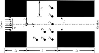
The computational domain, depicted in figure 1, has a cavity length
 $L$
, with a length over depth ratio
 $\unicode[STIX]{x1D6E4}=2$
, kept constant throughout the entire study. The inflow length is
 $L_{1}=0.6L$
and the outflow length is
 $L_{2}=1.2L$
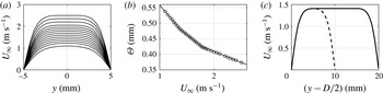
. Longer outflow lengths did not produce significant changes on the flow inside the double cavity. Usual Neumann boundary conditions are applied for solving the pressure Poisson equation. For the velocity, the inflow boundary conditions are of Dirichlet type, with an imposed velocity profile in order to control the flow rate. The outlet boundary conditions are defined by solving a simple one-dimensional advection equation along the normal direction to estimate the velocity profile in the outlet plane. The normal velocity component is then corrected such that the inlet flow rate is preserved. This simple approach ensures mass conservation and limits spurious effects on the solution at the vicinity of the outlet. The usual no-slip and impermeability conditions are applied at the walls. The laminar inflow profiles, imposed at the inlet boundary of the computational domain, were obtained considering an additional length of the upstream channels of
 $2.8L$
in which a laminar boundary layer develops on either side of the channel. A set of approximately 30 velocity profiles was created for each distance
 $D$
. The profiles for case
 $D/L=0.2$
and the variation of the momentum thickness
 $\unicode[STIX]{x1D6E9}$
with
 $U_{\infty }$
are depicted in figure 2(a,b), respectively. Inflow profiles for larger cavity distances are obtained by extending the
 $D/L=0.2$
profiles in the
 $y$
-direction, i.e. filling the resulting gap with the value of the respective maximum velocity. It is thus ensured that while
 $D$
is varied, the maximum velocity
 $U_{\infty }$
and the momentum thickness
 $\unicode[STIX]{x1D6E9}$
of the profiles are kept constant. Figure 2(c) shows an example of the extension of a
 $D/L=0.2$
to a
 $D/L=0.4$
case.
Computational domain of double cavity geometry with variable distance
 $D$
, inflow length
 $L_{1}=0.6L$
, cavity length
 $L$
, cavity aspect ratio
 $L/H=2$
, outflow length
 $L_{2}=1.2L$
and probe points
 $P_{1}$
–
 $P_{8}$
. Arrows indicate flow direction.

(a) Inflow velocity profiles for case with
 $D/L=0.2$
for different inflow velocities (for clarity not all velocity profiles are depicted). (b) Momentum thickness
 $\unicode[STIX]{x1D6E9}$
as a function of the maximum inflow velocity
 $U_{\infty }$
. (c) Extension of a
 $D/L=0.2$
profile (– –) to a
 $D/L=0.4$
profile (——).

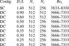
The domain is covered with 512 cells in the
 $x$
-direction, and 256 or 512, depending on
 $D$
, in the
 $y$
-direction. The grid convergence of the numerical scheme is of second order. The mesh is refined close to the walls of the inflow and outflow channel as well as in shear-layer regions and close to the impinging edge, in order to resolve the strong velocity gradients in these areas. The numerical simulations are carried out over a time duration of approximately 400–600 convective time units
 $\unicode[STIX]{x1D70F}_{c}=L/U_{\infty }$
, depending on the case. The code automatically adapts the time step size to ensure numerical stability, respecting
 $CFL=0.25$
, where CFL is the Courant number. As a reference for the double cavity (DC), a single cavity (SC) case is added, by closing one of the cavities at a distance of
 $D=1.4L$
. All simulated cases are summarized in table 1.
Summary of cases.

3 Time series
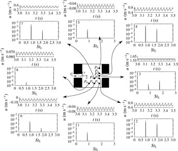
Probe points are located in various positions inside the domain, as indicated in figures 1 and 3. Time series are recorded at these probe points with a sampling frequency of approximately 5 kHz. The Strouhal number is defined as
 $St_{L}=fL/U_{\infty }$
, in which
 $f$
is the measured frequency. The initial 30 % of each time series is discarded in order to avoid transient effects. The Welch algorithm (Welch Reference Welch1967) with a window size of 5.1 s and an overlap of 98 % is used to compute the power spectral density (PSD) from the streamwise component of the velocity fluctuations. The spectral resolution is thus
 $\unicode[STIX]{x0394}St\approx 0.01$
. All power spectra depicted in this work are normalized by pre-multiplying with two times the frequency resolution:
 $2\text{PSD}\unicode[STIX]{x0394}f$
. Time series from eight probe points together with their power spectra are shown in figure 3 for a typical case. The same frequency (
 $St\approx 1$
) is amplified in the entire domain, which suggests that the spectrum is representative of the global dynamics. Hence, the spectral analysis of the different points can be reduced to a single point. Probe points
 $P_{2}$
and
 $P_{4}$
were chosen for most of the forthcoming spectral analyses, since they carry information from both the respective shear layers as well as the recirculation region. The reason why in point
 $P_{3}$
the second harmonic rises above its fundamental frequency will be explained later in the article. Inside the cavities, the second harmonic has smaller amplitudes than in the shear layer.
Time series of streamwise velocity component
 $u$
and its power spectral density from probe locations
 $P_{1}$
–
 $P_{8}$
of case
 $D/L=0.2$
at
 $Re_{L}=5100$
.

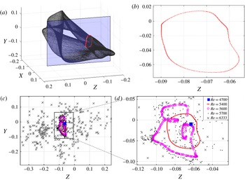
(a) Phase portrait: three-dimensional projection of the reconstructed flow from time series of
 $D/L=0.2$
case at
 $Re_{L}=5400$
using time delay embedding (
 $\unicode[STIX]{x1D70F}=0.015$
s). Vertical plane (blue) at
 $X=0.0055$
indicates position of the Poincaré section. Intersections of phase portrait with plane is indicated by red symbols. (b) Poincaré section: intersection of phase portrait in (a) with plane
 $X=0.0055$
. (c) Poincaré sections (
 $X=0.0055$
) at
 $Re_{L}=4700$
(blue filled square, periodic regime),
 $Re_{L}=5400$
(red solid line, intermediate regime (quasi-periodic case)),
 $Re_{L}=5600$
(magenta
 $\circ$
, folded torus),
 $Re_{L}=5700$
(black dots, low-order chaotic regime).
 $Re_{L}=6333$
(grey crosses, high-order chaotic regime). (d) Zoom-in view of (c).

3.1 Phase space analysis
Different regimes are encountered when the Reynolds number
 $Re_{L}$
is varied. We choose phase space representations to characterize these regimes. Phase space is reconstructed using time delay embedding of time series
 $s(t)$
(in our case the streamwise component of the fluctuating velocity) recorded at probe point
 $P_{2}$
. The three-dimensional projection of the reconstructed phase space, spanned by the time delayed vectors
 $$\begin{eqnarray}[X,Y,Z]^{\text{T}}=[s(t),s(t-\unicode[STIX]{x1D70F}),s(t-2\unicode[STIX]{x1D70F})]^{\text{T}},\end{eqnarray}$$
where
 $\unicode[STIX]{x1D70F}$
is the time delay, is shown in figure 4(a) for an illustrative case with
 $D/L=0.2$
. The time delay
 $\unicode[STIX]{x1D70F}$
was chosen such that the embedding dimension does not depend on
 $\unicode[STIX]{x1D70F}$
, using the method of Cao (Reference Cao1997). Other types of embedding techniques, such as single value decomposition (SVD) embedding, were tested, and the conclusions remain the same. Figure 4(b) depicts the Poincaré section, a two-dimensional subspace of the three-dimensional phase space in figure 4(a). It is obtained as an intersection of the plane at
 $X=0.0055$
with the phase portrait in figure 4(a). The Poincaré section was chosen transverse to the flow in the best agreement with the three conditions for a global Poincaré section (see Solari, Natiello & Mindlin Reference Solari, Natiello and Mindlin1996). Figure 4(c) exemplifies the Poincaré sections of the
 $D/L=0.2$
geometry for different Reynolds numbers. Figure 4(d) shows a zoomed-in view of figure 4(c). Based on these Poincaré sections, we can now define the flow regimes.
Once the flow evolves from the steady regime to the periodic regime, a period-1 limit cycle is reached in phase space and a single point can be observed in the Poincaré section (
 $Re_{L}\approx 4700$
). When the value of the Reynolds number is further increased (
 $Re_{L}\approx 5400$
), a so-called intermediate regime is reached. This regime includes quasi-periodicity, i.e. a second frequency appears in the spectrum, incommensurate with the dominant frequency. This induces the creation of a torus in phase space, which is characterized by a closed curve in the Poincaré section. Frequency locking may occur on the torus, resulting in periodic windows. At
 $Re_{L}\approx 5600$
the torus surface is folded by wrinkles. The Poincaré section of the torus presents self-intersections, indicating that the state space has at least a dimension equal to 4. The Cao (Reference Cao1997) algorithm, applied to the time signal in this flow regime gives an actual dimension of 5. This relatively small (local) dimension does not preclude potentially higher, though finite, dimensions for the full state space. For
 $Re_{L}\approx 5700$
, more complex dynamics is reached, though still structured around the torus. Finally, for Reynolds number
 $Re_{L}=6333$
, the Poincaré map yields a cloud of points (see figure 4
c) without any identifiable structure. The last two regimes are reminiscent of chaotic behaviour and hence are labelled chaotic regime. Yet note, that the dispersion of points in the Poincaré map alone is not a quantitative proof, though a strong indication of the chaotic nature of the system. The described route to chaos is common to small channel heights (
 $D/L<0.30$
) and is similar to the Curry & Yorke (Reference Curry, Yorke, Markley, Martin and Perrizo1978) scenario: steady (fixed) point
 $\rightarrow$
period-1 limit cycle
 $\rightarrow$
quasi-periodicity
 $\rightarrow$
torus breakdown leading to toroidal chaos, as also recently observed for the van der Pol system by Letellier, Messager & Gilmore (Reference Letellier, Messager and Gilmore2008). For larger channel heights (
 $D/L>0.35$
), however, the route to chaos looks slightly different, while configurations with
 $D/L=0.35$
and
 $D/L=0.30$
have their own distinctive details, as we shall see in the following sections. Henceforth, our so-called intermediate regime is not exclusive to quasi-periodic behaviour, as it may also include periodic windows, that occur due to frequency locking on the torus.
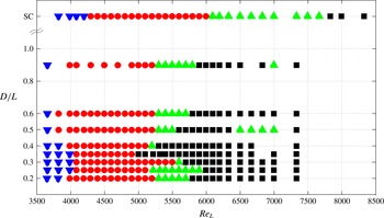
Parameter space plot. Blue ▾: steady regime. Red ●: Periodic regime. Green ▴: intermediate regime. Black ▪: chaotic regime. Note, the top line corresponds to a SC channel.

3.2 Parameter space
Based on the characterizations from § 3.1, a parameter space plot, depicted in figure 5, is constructed. It summarizes the regimes, found when the Reynolds number and the cavity distance are varied. Double cavity flow is equivalent to the canonical SC flow when the distance
 $D$
is very large. In general, the respective regimes are found at higher Reynolds numbers for SC flow when compared to DC flow. The steady regime is the first regime observed. It ends with the development of instabilities that produce self-sustained oscillations of the flow. The associated limit cycle is observed in our study for
 $Re_{L}$
lying in the range between
 ${\approx}3700$
and
 ${\approx}4300$
depending on the value of
 $D$
. The periodic regime is prone to develop at lower
 $Re_{L}$
for intermediate cavity distances (
 $D/L=0.5$
and
 $D/L=0.6$
) and at higher
 $Re_{L}$
for small (
 $D/L\leqslant 0.4$
) as well as for very large distances (
 $D/L\geqslant 0.9$
). The case
 $D/L=0.3$
is an exception to the other close distance cases: its periodic regime is observed for much larger Reynolds numbers, compared to its neighbours. Depending on the values of
 $D/L$
, the intermediate regime begins around
 $Re_{L}\approx 5500$
for the double cavity, while for the single cavity it starts at
 $Re_{L}\approx 6000$
. The Reynolds number range of the intermediate regime depends on the cavity distance. The longest range is found for the single cavity, while the shortest range is found for distances close to
 $D/L=0.35$
. At
 $D/L=0.35$
the intermediate regime disappears all together in what looks like a sudden (hard in amplitude) transition to chaos (Lopez-Rebollal & Sanmartin Reference Lopez-Rebollal and Sanmartin1995) and the chaotic regime is encountered in direct continuation to the periodic regime. However, it cannot be fully excluded that a quasi-periodic regime be recovered with a smaller step size in the value of the Reynolds number.
3.3 Spectral analysis
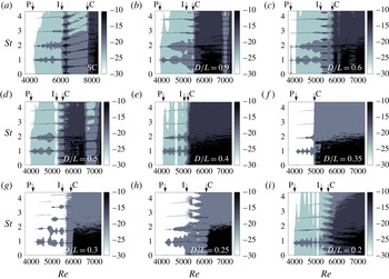
In this section we characterize the spectra associated with each regime. Figure 6(a–i) show the power spectra for all cases in table 1 when the Reynolds number is varied. In the steady regime no oscillations and hence no frequency peak is present. In the periodic regime, a salient peak at
 $St_{L}\approx 1$
prevails over a wide range of the Reynolds number. As expected, harmonics of this dominant mode are also present in the spectrum. The power spectra in these regions show strong dark lines equispaced in the vertical coordinate, reminiscent of the teeth of a ‘comb’. For
 $D/L\geqslant 0.4$
, when approaching the intermediate regime, the dominant Strouhal number
 $St_{L}\approx 1$
is gradually replaced by its first harmonic
 $St_{L}\approx 2$
. In the Poincaré section this is accompanied by an additional intersection. The underlying physics of this phenomenon will be addressed in § 4.2. In the intermediate regime, the peak at
 $St_{L}\approx 1$
, and its harmonics, are still present, but new peaks of incommensurate frequencies arise in the spectra, a phenomenon that is in correspondence with the creation of a torus in phase space mentioned in § 3.1. Peaks of much lower values of non-dimensional frequencies than the previous dominant Strouhal number indicate that a slow dynamics now leaves the signature in the spectrum. As a consequence of the rise of incommensurate frequencies, its harmonics and linear combinations, a tighter comb with a reduced teeth separation is observed in the power spectra of figure 6. Some exceptions may occur, as illustrated in figure 6(g,h). We may notice in these graphs a discontinuity in the evolution of the dominant frequency at
 $Re_{L}\approx 5000$
and
 $Re_{L}\approx 5300$
, respectively. The underlying physics of these discontinuities will be discussed in § 4.4. In the intermediate regime of the SC, the Strouhal number increases monotonically with the Reynolds number and the teeth are inclined. The trajectory in phase space is locked on the torus during most of the intermediate regime of the SC, resulting in a periodic window with
 $St_{L}\approx 0.5$
and its harmonics over a wide range of Reynolds numbers. In the spectra corresponding to the intermediate regime of the DC, the third and fourth peaks are in general in the ratio
 $\simeq 3/4$
. Furthermore, the first and third peaks keep a ratio of
 $\simeq 1/3$
. We will discuss the reason of this behaviour in § 4. With the exception of
 $D/L=0.35$
, all transitions to the chaotic regime take the quasi-periodic route. As the Reynolds number is further increased, the spectrum becomes richer, filling in with linear combinations of both incommensurate frequencies. Nonlinear effects promote the dynamics to enter the chaotic regime. At even higher Reynolds numbers, the spectrum eventually becomes much flatter, peaking at
 $St_{L}\approx 0.4$
. The decay of the time-correlation functions strongly indicates that the dynamics is chaotic in this regime. As expected when
 $Re_{L}$
is increased in the chaotic regime, chaos resorption may occur over finite windows of
 $Re_{L}$
. For instance, in figure 6(d) for the case
 $D/L=0.5$
, such a window is observed between
 $Re_{L}=6500$
and
 $Re_{L}=7000$
, where the spectrum simplifies and the flow returns from chaotic to the intermediate regime with
 $St_{L}=0.5$
. For
 $D/L=0.9$
a stability window occurs at
 $Re_{L}=7000$
. Also, windows of simplified spectra may appear even inside the periodic regime, as can be observed for instance for
 $D/L=0.4$
, at
 $Re_{L}\approx 4700$
, in figure 6(e).
Power spectra versus increasing ramps of the Reynolds number for (a) SC, (b)
 $D/L=0.9$
, (c)
 $D/L=0.6$
, (d)
 $D/L=0.5$
, (e)
 $D/L=0.4$
, (f)
 $D/L=0.35$
, (g)
 $D/L=0.3$
, (h)
 $D/L=0.25$
, (i)
 $D/L=0.2$
. Colour code depicts the normalized power spectra in log scale:
 $\log (2\text{PSD}\unicode[STIX]{x0394}f)$
. Arrows indicate where the periodic (P), the intermediate (I) and the chaotic (C) regime commence in each case.

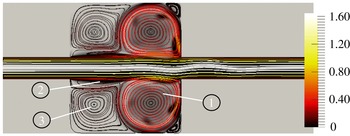
Instantaneous velocity flow field with streamlines of case
 $D/L=0.2$
at
 $Re_{L}=4900$
(periodic regime). Colour code of the streamlines correspond to the velocity magnitude. Background corresponds to vorticity magnitude. Numbers 1–3 indicate intracavity flow recirculation regions.

Flow patterns for the single cavity in the (a) steady regime, (b) periodic regime with
 $St_{L}\approx 1$
most amplified, (c) periodic regime with
 $St_{L}\approx 2$
most amplified, and (d) intermediate regime (quasi-periodic locked-on torus), together with respective time series recorded in probe point
 $P_{2}$
and its power spectra. Colour code indicates vorticity magnitude. For details on the ratio
 $p/q$
see text.

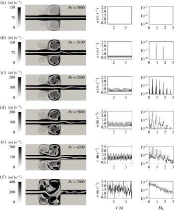
Flow patterns for case
 $D/L=0.2$
in (a) steady regime, (b) periodic regime (limit cycle), (c) intermediate regime (torus), (d) intermediate regime (torus folding), (e) chaotic regime (toroidal chaos), and (f) chaotic regime (exploded torus) together with time series recorded in probe point
 $P_{2}$
and respective power spectra. Colour code indicates vorticity magnitude.

4 Flow field analysis
In this section, the dynamical system analysis is linked to the flow dynamics. We first discuss the salient characteristics of the flow structure. As we see in figure 7, in each cavity, the inner flow is structured in two large main recirculation regions and a third smaller one. The main recirculation region, located in the downstream half of the cavity, remains almost circular up to the end of the intermediate regime. The secondary recirculation, located in the upstream half of the cavity, is also closely circular. The line connecting the centres of recirculation regions 1 and 2 (cf. figure 7) is parallel to the free-stream direction. The dynamics of both recirculation regions is however quite different, as the magnitude of the velocity field in the secondary recirculation region is one order of magnitude smaller than in the main recirculation region. The third, smaller, recirculation bubble is located on top of the secondary recirculation region, below the shear-layer close to the leading edge. These observations are in agreement with Mizushima & Shiotani (Reference Mizushima and Shiotani2001), who found essentially the same flow pattern for a geometry with a slightly greater cavity aspect ratio
 $\unicode[STIX]{x1D6E4}=L/H=2.6$
.
The vorticity magnitude field is plotted in figures 8 for the single cavity flow, and in figure 9, for the
 $D/L=0.2$
DC flow, for different Reynolds numbers, with time series of the signal, recorded in probe point
 $P_{2}$
and the associated power spectra. For low Reynolds numbers,
 $Re\lesssim 4000$
, the flow is steady. A circular dipolar vortex sheet limits the main recirculation region, as can be seen for instance in figures 8(a) and 9(a). In the periodic regime, the shear layer exhibits oscillations of such magnitude that vorticity of the shear layer is regularly injected at the rear edge of the cavity into the main recirculation region. The injected vorticity forms small vortices at the frequency of the shear-layer oscillations. These regularly spaced vortices circumvent along the dipolar vortex sheet, creating a ‘carousel’ type formation. The number of small vortices in the carousel depends on the value of
 $D$
and on the velocity of the incoming flow, which defines the frequency at which the shear layer oscillates, and hence the rate at which small vortex structures are injected into the cavities. The vorticity strength of these vortices decreases along their circular motion in the carousel. The existence of these small vortices is readily seen in the spectrum. They leave a signature on the probe signal as a consequence of their cyclic passage.
Henceforth, the analysis will focus on the interaction of the shear layer with the main recirculation region.
4.1 Characteristic time scales
Different time scales of interest appear in this phenomenon. We define
 $T_{shl}$
as the characteristic time of the prevailing oscillations of the shear layer,
 $T_{to}$
the turnover time of the main recirculation region, and
 $T_{lt}$
the characteristic lifetime of the small vortex structures. The advective time
 $\unicode[STIX]{x1D70F}_{c}=L/U_{\infty }$
is the natural reference time. It turns out that
 $T_{shl}/\unicode[STIX]{x1D70F}_{c}\simeq 1$
in all cases. If the main recirculation region was considered as being driven only by the shear layer in solid rotation,
 $T_{to}$
should scale with
 $U_{\infty }$
and
 $H$
. In this respect, one could therefore expect that
 $T_{to}\unicode[STIX]{x1D6E4}/\unicode[STIX]{x1D70F}_{c}$
also be little sensitive to the value of
 $Re_{L}$
. However, this is not the case. Instead, we observe a dependence of both
 $T_{to}\unicode[STIX]{x1D6E4}/\unicode[STIX]{x1D70F}_{c}$
and
 $T_{to}/T_{shl}$
with
 $Re_{L}$
. The ratio
 $T_{to}/T_{shl}$
depends additionally on the momentum thickness
 $\unicode[STIX]{x1D6E9}$
of the incoming boundary layer, which defines the shear-layer thickness, among other parameters that will be further clarified. The lifetime
 $T_{lt}$
is not easily determined as it is a function of the viscosity of the fluid, of the strength of the small vortices and of their interaction with the neighbouring vorticity. A reference time can be considered assuming
 $T_{lt}\sim \unicode[STIX]{x1D702}^{2}/\unicode[STIX]{x1D708}$
where
 $\unicode[STIX]{x1D702}$
is the radius of the small vortices, which depends on the amplitude of the shear-layer oscillations and therefore on
 $Re_{L}$
. The ratio
 $T_{lt}/T_{to}$
determines, whether in a single snapshot of the vorticity field, the small vortices in the image were all created in the same round trip (figure 8
a), or vortices from two or more consecutive round trips coexist (figure 8
c,d).
4.2 Flow field dynamics of the periodic regime
For the periodic regime, the simplest configuration is obtained when
 $T_{lt}<T_{to}$
, i.e. the small vortices dissipate before they complete one round trip in the carousel. Figure 8(b) illustrates this configuration, for the SC flow, where seven small vortices are formed during one turnover cycle (
 $T_{to}/T_{shl}\simeq 7$
). These vortices have such a small lifetime, that during one cycle they do not appreciably reach the region of vorticity injection. The only frequency measured in probe point 2 is therefore the frequency of the shear-layer oscillations.
For
 $2T_{to}\gtrsim T_{lt}\gtrsim T_{to}$
, the vortex completes one round trip and returns to the injection position, exiting the shear layer in a feedback process. A periodic regime may still be encountered in this case over a wide range of the
 $Re$
number. In such a situation, both the shear-layer oscillations and the carousel turnover are synchronized, which is something usually expected from two coupled oscillators. Periodic behaviour implies
 $T_{to}/T_{shl}=p/q$
, with
 $p,q\in \mathbb{N}$
and
 $p>q$
. Many different possible scenarios are found in SC and DC flows, depending on the values of
 $Re_{L}$
, ratio
 $T_{to}/T_{shl}=p/q$
, and
 $D$
. We shall illustrate some of them below.
In figure 9(b) we observe, for a DC flow case, a situation in which
 $T_{to}/T_{shl}=4$
. The vorticity plots show four small equispaced vortices per cavity in the main recirculation region. The structures of the carousels of each cavity are in opposite phase. Once a small vortex returns to the area of injection at the rear edge of the respective cavity, the shear layer injects a new vortex in its position. The power spectrum exhibits in this case the main peak at
 $St_{L}\simeq 1$
, as the cyclic passage of the different vortices at probe position occurs at the frequency of the shear-layer oscillations. The amplitude of the first harmonic is enhanced by the opposed carousel. The set of two carousels, exhibiting phase opposition, produces a signal that doubles the frequency of the shear layer. This is clearly illustrated in the spectrum of figure 3 at probe point
 $P_{3}$
. There, the peak at
 $St\simeq 2$
is of larger amplitude than the peak at
 $St\simeq 1$
.
Figure 8(c) illustrates the case of an extremely large value of
 $D/L$
or equivalently a single cavity flow. For this case the ratio is
 $T_{to}/T_{shl}=7/2$
and the dynamics is periodic. The power spectrum exhibits a dominant peak at
 $St_{L}\simeq 2$
in probe point
 $P_{2}$
, while a peak at
 $St_{L}\simeq 1$
is still present. The reason for this spectral distribution, is that
 $T_{lt}/T_{to}\simeq 2$
. Consequently, the carousel is made of two intertwined patterns of small vortices, which doubles the frequency in
 $P_{2}$
. The first pattern is weakened since it enters its second turn in the recirculation region, while the second pattern carries a stronger vorticity as it enters for the first time (figure 8
c).
The ratio
 $T_{to}/T_{shl}$
, however, evolves as the
 $Re$
number is increased. By further increasing
 $Re_{L}$
, the single cavity reaches a periodic regime with
 $St_{L}\simeq 0.5$
in which
 $T_{to}/T_{shl}=10/3$
. A snapshot of this flow regime is shown in figure 8(d). Due to
 $T_{lt}/T_{to}\simeq 2$
the carousel pattern, though still periodic, becomes more complex.
To summarize, a periodic regime is obtained for either (i)
 $T_{lt}<T_{to}$
or (ii)
 $T_{lt}\geqslant T_{to}$
when at the same time
 $T_{to}/T_{shl}=p/q$
, with
 $p,q\in \mathbb{N}$
. In the first case the rhythm is set by the shear layer, since the small vortices dissipate before completing one round trip in the carousel. In the second case, the shear layer and the carousel are locked in by
 $T_{to}/T_{shl}=p/q$
, with
 $p,q\in \mathbb{N}$
. We did not observe cases with
 $T_{lt}\gtrsim 2T_{to}$
in the periodic regime.
4.3 Flow field dynamics of the intermediate regime
In the intermediate regime, incommensurate frequencies appear in the spectrum and the trajectory in phase space lies on a torus. We can expect that this new behaviour manifests itself in the dynamics of the carousel. We have shown in § 3.3, that many different situations are encountered in the intermediate regime. Rather than describing all the possible scenarios, let us instead illustrate some examples.
For
 $D/L=0.2$
at
 $Re=5500$
(figure 9
c), the lifetime of the small vortices lasts approximatively two turnover times
 $T_{lt}\simeq 2T_{to}$
before they dissipate. The carousel pattern exhibits recurrent states with
 $n=3$
or
 $n=4$
vortices. Expressed in terms of time scales we get:
 $3<T_{to}/T_{shl}<4$
. The small vortices are not equispaced as a consequence of the continuous transitions between both states. The spectrum displays the frequency associated with the shear-layer instability at
 $St_{L}\approx 1$
and a second incommensurate frequency
 $St_{L}\approx 0.45$
associated with the carousel’s patterns.
Continuing with figure 9(d) at
 $Re_{L}=5800$
, the three vortex pattern per cavity prevails. The spectrum shows both the frequency associated with the shear-layer oscillations (
 $St_{L}\approx 1$
) and with the passage of the three small vortices. The frequency ratio between the values of the frequencies of the third and fourth modes, which is
 $\simeq 3/4$
, can be associated with the recurrence in each cavity of a three vortex pattern instead of a four vortices pattern, synchronized with the shear-layer instability. The ratio of the new peaks, at
 $St_{L}\simeq 0.45$
and
 $St_{L}\simeq 1.35$
, reaches a value close to
 $1/3$
that can be associated with the cyclic behaviour of the three vortex pattern in the intracavity structures.
At Reynolds number close to
 $6200$
(figure 9
e), the intermediate regime loses coherence and the small vortices are not regularly spaced anymore. Note however, that the vortex carousel persists. Finally, at Reynolds numbers close to 7000 (figure 9
f), the recirculation regions deform strongly. The recurrent patterns of vortices in the carousel become largely disordered and are not easily determined. In fact, the vortices injected into the cavities by the shear layers are of such intensity, that after one turnover, they largely disturb the incoming shear layer and make the periodic feedback mechanism impossible. The counterpart in phase space, to this last dynamics, is the torus breakdown (cf. figure 4).
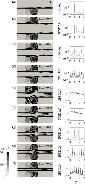
Flow patterns for different cavity distances
 $D/L$
at
 $Re=5500$
and the respective power spectra from time series recorded in probe point
 $P_{2}$
. Colour code indicates vorticity magnitude. (a) Periodic regime, (b) intermediate regime, (c) intermediate regime, (d) intermediate regime, (e) chaotic regime, (f) chaotic regime, (g) periodic regime, (h) intermediate regime, and (i) intermediate regime.

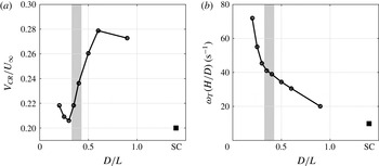
(a) Normalized carousel speed
 $V_{CR}$
and (b) angular velocity
 $\unicode[STIX]{x1D714}_{T}=V_{CR}/(H/2)$
multiplied by the depth over distance ratio
 $H/D$
as a function of the normalized cavity distance
 $D/L$
for all cases in figure 10 (
 $Re=5500$
). The SC case is indicated by ▪. The shaded areas indicate the distances for which chaotic behaviour occurs (see figure 10).

4.4 Coupling strength
Let us consider the spatial symmetry of the two-dimensional vorticity magnitude field
 $|\unicode[STIX]{x1D714}(x,y)|$
in figure 10. Considering a spatial reflection symmetry (with respect to the centreline
 $y=0$
), we distinguish between the following two cases:
 $$\begin{eqnarray}\left.\begin{array}{@{}l@{}}|\unicode[STIX]{x1D714}(x,y)|=|\unicode[STIX]{x1D714}(x,-y)|\Rightarrow \text{spatially symmetric (or varicose)}\\ |\unicode[STIX]{x1D714}(x,y)|\neq |\unicode[STIX]{x1D714}(x,-y)|\Rightarrow \text{spatially asymmetric}.\end{array}\right\}\end{eqnarray}$$
Note, in the periodic regime the spatially asymmetric cases correspond to a sinuous flow configuration. Both symmetric and asymmetric cases are observed, though in most cases the flow is of the asymmetric type. For a given Reynolds number, as
 $D/L$
is varied and the coupling between the cavities evolves, the flow symmetry may change. This is illustrated in figure 10 for
 $Re_{L}=5500$
. For close facing cavities, when
 $D/L<0.25$
, the flow configuration is spatially asymmetric. The symmetry changes as
 $D/L$
increases and gets closer to
 $D/L=0.3$
, a value for which the flow adopts a spatially symmetric (varicose) configuration. Increasing
 $D/L$
again, the flow returns to a spatially asymmetric configuration. The emergence of spatial symmetry explains the discontinuity in the Strouhal number as a function of the Reynolds number for
 $D/L=0.25$
at
 $Re_{L}=5400$
and
 $D/L=0.3$
at
 $Re_{L}=5000$
, respectively (cf. figure 6
g,h). At these Reynolds numbers the flow adopts the varicose flow configuration. For the case
 $D/L=0.3$
the change in symmetry occurs in the periodic regime without hysteresis, while for the case
 $D/L=0.25$
the change in symmetry is located in the intermediate regime and a hysteresis was observed. The change in symmetry before the transition to unsteady or turbulent flow conditions was also observed for the flow past a sphere by Johnson & Patel (Reference Johnson and Patel1999) and Tomboulides & Orszag (Reference Tomboulides and Orszag2000).
Let us analyse the interaction of the feedback mechanisms of the carousel as we modify the ratio
 $D/L$
for a fixed value of Reynolds number. For
 $Re_{L}=5500$
, the flow passes through all regimes as
 $D/L$
is varied. As exemplified in figure 10(a), the number of small vortices in each recirculation region is four when the cavities are infinitely far from each other (SC). This corresponds to a case in which
 $T_{to}/T_{shl}=4$
and
 $T_{lt}\simeq T_{to}$
and the recorded value compares favourably with the average recirculation velocity reported by other researchers (Villermaux & Hopfinger Reference Villermaux and Hopfinger1994; Back & Roschke Reference Back and Roschke1972). A noticeable change in the carousel is observed, when a second cavity is present at proximity (figure 10
b–d). We observe, that the frequency is almost constant but the number of small vortices in the carousel diminishes, which means that the carousel must turn faster, since the shear-layer instabilities can not be strongly modified, as neither the Reynolds number nor the momentum thickness have changed. Figure 11(a) shows the carousel speed, normalized with the centreline velocity
 $U_{\infty }$
, as a function of the cavity distance. We observe, that the second cavity has a strong effect. The carousel speed increases by 43 %, when
 $D/L$
is varied from 1.4 (SC) to 0.9 (DC). This increase in angular velocity has in turn a critical effect on the feedback mechanism between the carousel and the shear layer. Although the carousel is turning faster, the lifetime of the circumventing vortices has not been significantly modified. As a consequence, the injected vortices remain strong when they come back to the shear-layer region, which they now excite. As a result, the amplitude of the shear-layer oscillations is reinforced by this excitation, and the vorticity injected into the carousel at the impingement, becomes stronger. Mutual induction between the stronger and (relatively) long living circumventing vortices can further increase their speed in the carousel. Indeed, the angular velocity of the carousel increases as
 $D/L$
is reduced and reaches a maximal value for
 $D/L\approx 0.6$
. For more contiguous cavities, the angular velocity of the carousel decreases again. This may be understood as a ‘blocking’ effect due to the proximity of the shear layer of the facing cavities. The shaded zones in figure 11 indicate the
 $D/L$
-range for which chaotic behaviour is observed. The speed drops to a minimum when
 $D/L=0.3$
, the distance at which the flow becomes symmetric, as can be seen from figure 10(g). The carousel speed slightly increases for the closest distances (cases
 $D/L=0.25$
and
 $D/L=0.2$
). In figure 11(b) the angular velocity, multiplied by the depth to distance ratio, is plotted against the normalized cavity distance
 $D/L$
. Interestingly, the resulting curve decreases monotonously, while the trend for
 $V_{CR}$
, as a function of
 $D/L$
, is quite different, as shown in figure 11(a). Note however, that
 $\unicode[STIX]{x1D714}_{T}$
and
 $V_{CR}$
are connected through the relation:
 $$\begin{eqnarray}\unicode[STIX]{x1D714}_{T}\frac{H}{D}=\frac{V_{CR}}{H/2}\frac{H}{D}.\end{eqnarray}$$
The change in the carousel speed is even more striking when
 $D/L$
is fixed and the Reynolds number is varied. In the SC, for instance, the number of circumventing vortices in the carousel changes from
 $n=7$
to about
 $n=3$
when the Reynolds number passes from 4600 to 5100, as can be seen in figure 8. The relative change in the incoming flow velocity is approximately 10 % while the turnover time increases by 50 %. This behaviour is common to all cases. The significance of the carousel mechanism to understand the coupling between shear-layer and intracavity flow and also to understand the mutual interactions between facing cavities, encourages future work on the subject.
Experimental evidence of the vortex carousel can be found in the literature for open cavity flow by e.g. Basley et al. (Reference Basley, Pastur, Lusseyran, Faure and Delprat2011) and Basley et al. (Reference Basley, Pastur, Delprat and Lusseyran2013). In these works, smoke visualizations and particle image velocimetry measurements for a
 $\unicode[STIX]{x1D6E4}=L/H=1.5$
cavity show the mechanism. The length to depth ratio
 $\unicode[STIX]{x1D6E4}$
most likely does become important for
 $\unicode[STIX]{x1D6E4}\gg 2$
, as in Mizushima & Shiotani (Reference Mizushima and Shiotani2001) and Mullin et al. (Reference Mullin, Shipton and Tavener2003), who showed that the flow field can become heavily asymmetric due to large cavity lengths
 $L$
. Such an asymmetry will certainly alter the carousel mechanism.
4.5 The outflow pattern
It is also interesting to observe how the flow is modified at the exit channel as the different regimes take place (cf. figure 9). The outflow in the steady regime and in the periodic regime is well organized and the presence of the double cavity does not introduce significant modifications between the inflow and the outflow. As the Reynolds number is increased and the intermediate regime begins, the outflow becomes more complex and once the chaotic regime is reached, strong mixing is produced. As a potential application, DC flow could hence be designed as a laminar chaotic mixing device. In figure 5, we can observe that the chaotic regime for DC flows is reached at much lower Reynolds numbers for closer cavity distances. This reflects the consequence of the strong coupling of the two individual cavities, and the advantage of a DC configuration when mixing enhancement is pursued.
5 Conclusions
We studied a system, composed of two facing cavities, driven by a flow entering from a channel that determines the characteristics of the velocity profile at the leading edge of the cavities. We restricted our analysis to cases in which the inflow profile was laminar, in order to exclude possible excitations associated with the intrinsic fluctuations of turbulent flows. A first analysis, considering time series of the velocity signal from two-dimensional numerical simulations, was carried out. We found that the signal of a single probe was in general rich enough to capture the salient features of the global behaviour. On this basis, a study was performed using time series from a single probe. As
 $Re_{L}$
is increased, for a given ratio
 $D/L$
, we found the following successive regimes: steady
 $\rightarrow$
periodic
 $\rightarrow$
intermediate
 $\rightarrow$
chaotic. A map was constructed which enables to identify these regimes for different Reynolds numbers and different separation distances between the cavities. In phase space, the periodic regime describes a limit cycle with a spectrum, that always exhibits a peak at
 $St_{L}\approx 1$
. In most cases, the oscillations of the shear layer is of the asymmetric type. The periodic regime is observed for
 $Re_{L}\gtrsim 4000$
, though this value depends on the cavity distances. For
 $D/L=0.5$
and
 $D/L=0.6$
it is reached at somewhat lower Reynolds numbers. As the Reynolds number is increased, the limit cycle disappears and the trajectories in phase space lie on a torus. The spectra become more complex, exhibiting combinations of the two basic incommensurate frequencies. Frequency lockings and un-lockings may occur on the torus, before it breaks down and bifurcates towards a chaotic regime. In this last regime, any phase coherence between the two shear layers is lost and oscillation amplitudes are one order of magnitude above the amplitudes of the periodic regime. We could verify that the transitions to the chaotic regime in almost all cases take the quasi-periodic route, in which a frequency smaller than the dominant Strouhal number appears. This route to chaos is reminiscent of a Curry & Yorke (Reference Curry, Yorke, Markley, Martin and Perrizo1978) scenario.
A second analysis was carried out, focusing on the vorticity fields, in order to link the phase space dynamics to the dynamics of the physical space. The visualization of patterns of small intracavity structures serves to understand the underlying mechanisms of the feedback process and helps to identify the flow regime. The small vortices are created as a consequence of the shear-layer oscillations, which regularly inject vorticity at the rear edge of the cavities. They describe a quasi-circular motion inside the main intracavity recirculation region, forming a ‘carousel-like’ structure in each cavity. These vortices, when returning to the region of the instability onset, excite the shear layers. The relative phase synchronization of the carousels indicates the degree of coupling between the two cavities. The angular velocity of the carousel and the number of vortices present in the carousel depend, non-trivially, on the Reynolds number and the distance between the cavities.
The interplay of three characteristic time scales determines the properties of the observed phenomena: the turnover time of the main recirculation region, the lifetime of the small intracavity vortices and the period of the shear-layer oscillations. We illustrated the importance of these three time scales on the dynamics of the physical space and the associated dynamics of the phase space. The simplest scenarios correspond to lifetimes so short, that the vortices cannot accomplish one complete round trip in the carousel. In this situation, time series indicate a periodic regime with
 $St_{L}\approx 1$
, associated with the shear-layer oscillations. When the lifetime is long enough, the small circumventing vortices keep an intensity capable to excite the shear layers, and therefore to produce a significant feedback process. Depending on the separation
 $D/L$
, the small vortices may even leave their signature in the signal of probes placed in the facing cavity. A periodic regime may be found for lifetimes larger than the turnover time, when the carousel synchronizes in such a way that any new vortex superposes with a dissipating one. When new vortices are injected in the space between two circumventing vortices, which have already completed one round trip, the spectrum reflects the frequency of the injection (
 $St_{L}\approx 1$
) and of the surviving carousel structures. Lifetimes up to two round trips were observed, which explains the complex spectral composition found for the intermediate regime. The chaotic regime occurs when the feedback process becomes too strong: the vortices of the carousel do not decay sufficiently and do not synchronize with the natural oscillations of the shear layer. Experimental evidence of the vortex carousel mechanism can be found in literature for open single cavity flows.
Our study raises questions that call for further research:
-
(i) Two-dimensional simulations indicate that there is a narrow range in
 $D/L$
where it is possible to find a symmetric (varicose) flow configurations. This state inhibits the intermediate regime and the flow stays in the periodic regime up to higher Reynolds numbers. It would be of interest to understand why the selection of this state occurs in such a narrow range in a two-dimensional context and if this state effectively occurs in three-dimensional flows.
-
(ii) When the inflow is laminar, there are no experimental reports of the chaotic regime for single cavity flows. However, this cannot be excluded as this requires specially designed experiments with well-controlled inflow conditions. Yet, a reduction of the lifetime of the small vortices related to a non-zero spanwise velocity component, seems another plausible reason for the absence of the chaotic regime.

Specifically dedicated experimental and/or numerical efforts seem necessary to clarify these points.
Acknowledgements
We wish to thank Dr Y. Duguet for the fruitful discussion and his valuable comments. We acknowledge support by CONICET (Argentina) under grant no. 3303, UBACYT under grant no. 100228, Science-Accueil d’Université Paris-Sud, LIA-PMF/FMF and the 13STIC-08-P-MVP project of the SticAmSud program. Furthermore F.T. greatly acknowledges the support of his PhD thesis by CONICET (Argentina), Université Paris-Sud & Université Saclay (France), Erich-Becker-Studienstiftung (Germany), and the DAAD (Germany).