1. Introduction
Maritime shipping remains the mainstay supporting international merchandise trade and globalisation owing to nearly 90% of international commodity trade being transported by maritime shipping (Kaluza et al., Reference Kaluza, Kölzsch, Gastner and Blasius2010). Growth in trading by sea converts into the growing need for more vessels, larger freight capacity and bigger travelling velocity, which emphasises concerns in the security management of maritime transportation (Tu et al., Reference Tu, Zhang, Rachmawati, Rajabally and Huang2017). Thus, the understanding of ship movements and vessel risk analysis has become increasingly important topics of research for their direct implication on maritime security and safety to decrease the emergence of water accidents (Alessandrini et al., Reference Alessandrini, Mazzarella and Vespe2018). Various qualitative and quantitative risk estimation approaches (maritime accident occurrence frequency, consequence severity evaluation, contributing indicator identification) have been developed over the past few decades (Li et al., Reference Li, Meng and Qu2012). Although these methods have a certain attraction, there are still some problems in practical application in coping with risk assessments in the real-time maritime environment (e.g. intersecting sea lanes, multi-modal collision avoidance behaviour) owing to most of these previous studies performing risk assessments based on ship pairs. These problems impede the actual contribution and practical application of risk estimation approaches in complicated dynamic navigation situations with irregularly approaching vessels. Thus, new nearly automatic risk evaluation approaches incorporating the spatial–temporal travelling behaviour of multi-ships are urgently required for real-time dynamic maritime traffic environment awareness.
The Automatic Identification System (AIS) is the nearly real-time tracking system equipped on ships and adopted by water traffic services to avoid ship collisions by way of the exchange of navigation information between ships electronically, with the support of onboard transceivers, as well as satellite and terrestrial base stations. The collected data consist of lots of information, such as kinematic (such as longitude, latitude, speed, time and course) and static (such as ship name, MMSI, ship size, ship type and ship flag) information. This information is beneficial for maritime security and safety by providing spatiotemporal and geographically distributed vessel positioning data and target recognition for collision avoidance by water transport (Tu et al., Reference Tu, Zhang, Rachmawati, Rajabally and Huang2017; Fang et al., Reference Fang, Yu, Lu, Feng and Huang2018b; Evmides et al., Reference Evmides, Odysseos, Michaelides and Herodotou2022; Felski and Jaskólski, Reference Felski and Jaskólski2012; Felski et al., Reference Felski, Jaskólski and Banyś2015; Öztürk et al., Reference Öztürk, Boz and Balcisoy2021; Rong et al., Reference Rong, Teixeira and Soares2022; Rothmund et al., Reference Rothmund, Haugen, Veglo, Brekke and Johansen2023; Tsou, Reference Tsou2016; Vestre et al., Reference Vestre, Bakdi, Vanem and Engelhardtsen2021; Yu et al., Reference Yu, Murray, Fang, Liu, Peng, Solgi and Zhang2022; Yu et al., Reference Yu, Bai and Liu2023b; Xin et al., Reference Xin, Liu, Loughney, Wang, Li and Yang2023a; Xu et al., Reference Xu, Wu, Xie, Teixeira and Yan2023). AIS also can support vessel collision risk diagnosing, modelling and simulation, as well as prediction and providing alerts, and become a keystone of maritime situational awareness (d’Afflisio et al., Reference d’Afflisio, Braca and Willett2021; Last et al., Reference Last, Hering-Bertram and Linsen2019; Mandal et al., Reference Mandal, Nagarajan and Sha2018; Murray and Perera, Reference Murray and Perera2020; Murray and Perera, Reference Murray and Perera2021; Murray and Perera, Reference Murray and Perera2022; Silveira et al., Reference Silveira, Teixeira and Soares2022; Szłapczyński and Niksa-Rynkiewicz, Reference Szłapczyński and Niksa-Rynkiewicz2018; Wright et al., Reference Wright, Janzen, Bochenek, Austin and Page2019; Xiao et al., Reference Xiao, Fu, Zhang and Goh2019; Yu et al., Reference Yu, Meng, Fang, Liu and Xu2023a; Zhao and Fu, Reference Zhao and Fu2021; Xiao et al., Reference Xiao, Li, Yao, Chen and Hu2022; Xin et al., Reference Xin, Yang, Liu, Zhang and Wu2023b). Thus, AIS-based trajectory data record the spatial-temporal movements of all ships in the study area suited well to be used in extending the physical and practical application analysis of multi-ship behaviour-oriented dynamic risk assessments considering heavy travelling environments.
Both data and methodology, which are closely related to each other, play critical roles in the intelligent maritime transportation system. Various methodologies in collision avoidance risk assessment require examination and validation with real-world true data for improving the capability, applicability and efficiency of dealing with real-world tasks. Similarly, real-world data are meaningless, and its value is hard to be completely taken advantage of without a series of appropriate methodologies. Therefore, an environment–kinetic compound space–time prism (EKC-STP) is presented with allowing moving objects considering resistance from kinetic and environmental restrictions, which can be adapted to multi-ship collision avoidance in complicated restricted areas.
Intense maritime traffic in port may cause highly changeable marine transportation, complex vessel spatiotemporal travel behaviours and significant navigational challenges. The complicated marine real-time environments mean the risk process between ship pairs is limited in the need for a new solution on near-real-time risk modelling and prediction for multi-candidate vessels. Thus, this study proposes the EKC-STP-based novel approach for modelling spatiotemporal interactions of multi-ship crossing avoidance taking the ship movement characteristics and travel context of restricted sea area into account, which improves the applicability and efficiency of the near-miss collision risk evaluation in port. The major contributions of the proposed methodology can be summarised and reviewed as follows.
-
1. The EKC-STP can measure possibilities of interaction of not only one encounter pair but also multi-ships by calculating the overlapping volumes, which improves the physical realism compared with other methods based on bound speed and direction of ships with static and dynamic obstacles.
-
2. The proposed EKC-STP develops a novel approach for modeling the near-miss collision risks by quantifying spatiotemporal interactions of multiple encountering ships, as well as incorporating the complicated movement environment context (e.g. multi-ships encounters, depth of water, land, shallows, buildings areas and maricultural zones).
-
3. The proposed model considers the velocity and course variations of encountered ships, and speed loss when turning to avoid a collision, as well as the travel environment characteristics, which is more effective and practical for identifying the proactive collision risk indicators related to real-time complicated water traffic.
-
4. This approach provides a new way to determine near-miss collision risks during unsampled periods between anchor points quantitatively and will be able to reveal when, where and how often ships were likely to have interacted if it is capable of getting the whole data set of AIS trajectories.
2. Literature review
Maritime ship movements have certain differences with the traffic movements on the road, for instance, ship travelling is mainly forced by the demand of the existing less subjective initiative. Urban traffic movements are restricted by the road network, and maritime ship movements are constrained by direction, static obstructions (i.e. land, shallows, etc.) and dynamic obstacles (i.e. depth of water and moving targets). Human activities have attracted extensive attention from scholars specialised in interdisciplinary areas of geographic information science and traffic. However, maritime transport activities have rarely been considered by interdisciplinary researchers. Thus, this paper tries to propose a heuristic methodology named EKC-STP for quantifying spatiotemporal interactions of multi-ship collision avoidance by including time geography in ship collision risk estimation, which shows good potential in situational awareness of complicated traffic environments. The related research on vessel collision risk estimation and quantitative space–time prism formulation is illustrated in the following subsections.
2.1. Collision risk estimation
Vessel collision risk assessment is crucial for safe vessel navigation and water security management due to possible high-influence consequences, including fatality, financial losses, extensive pollution and ship hull damage (Karahalios, Reference Karahalios2014; Celik et al., Reference Celik, Lavasani and Wang2010; Yu et al., Reference Yu, Fang, Murray and Peng2021a; Lyu et al., Reference Lyu, Hao, Li, Li, Sun, Zhang, Yin, Zhao and Zhang2023). Individual encounter ships’ collision risk modelling and regional risk distribution assessment mutually facilitate each other.
Current research on collision risk modelling for individual encounter ships is supported by vessel collision risk measurement and behaviour-oriented simulation methodologies. The vessel collision risk measurements comprise ship safe boundary involved risk level definition, manoeuvrability parameters driven risk functions and the combination of the aforementioned two methods.
Ship safe boundary involved risk level definition includes ship domain models (e.g. circular, elliptical (Wu et al., Reference Wu, Mehta, Zaloom and Craig2016), empirical (Hansen et al., Reference Hansen, Jensen, Lehn-Schiøler, Melchild, Rasmussen and Ennemark2013), knowledge-based, fuzzy (Qu et al., Reference Qu, Meng and Suyi2011), probabilistic, quaternion (Wang, Reference Wang2010; Liu et al., Reference Liu, Hu, Liang, Li, Liu and Yang2023; Lyu et al., Reference Lyu, Liu, Guo, Tan, Fu, Sun, Zhao, Zhang and Yin2024), and projected (Goerlandt and Kujala, Reference Goerlandt and Kujala2014) domains), multi-ship and collision diameter (e.g. Fujii (Fujii and Tanaka, Reference Fujii and Tanaka1971), Pedersen (Reference Pedersen1995) and COWI (Vessel, Reference Vessel2008)) to direct navigators to keep a certain distance from nearby ships. The ship domain is used for collision candidates detection based on minimum safety passing and early warning boundaries, as well as safety domain violation and overlapping (Qu et al., Reference Qu, Meng and Suyi2011; Christian and Kang, Reference Christian and Kang2017). The collision diameter has extensive applications, for example, estimating potential intersections between routes, more than collision risk estimation for encountering ships (Mou et al., Reference Mou, Van der Tak and Ligteringen2010). Ship domain and collision diameter are determined through statistical analysis of the particular navigational situation in certain water areas and are always associated with subjective expert knowledge, for instance, the choices of the investigated crew. In addition, an asymmetric warning signal is transmitted in the encounter situation.
The second catalogue in manoeuvrability parameters-driven risk functions integrates Distance (DCPA) and Time (TCPA) to the Closest Point of Approach, relative distance, course and azimuth deviation between encountering ships (Nguyen et al., Reference Nguyen, Zhang and Wang2018). The relative speed, course and distance-driven model for near-miss collision risk (Fang et al., Reference Fang, Yu, Ke, Shaw and Peng2018a; Zhang et al., Reference Zhang, Goerlandt, Montewka and Kujala2015) and the overlapping of velocity between obstructions and ships have also been applied in the collision risk estimation. The considered variables, formulation and relationship (e.g. linear and nonlinear) are all various. However, it is very hard to isolate the specific influence of a certain parameter from the comprehensive effect of multiple parameters. Furthermore, improvements are essential due to these parameters greatly depending on the reference ship.
The full consideration of the safe-navigation boundary and manoeuvrability parameters for different ships can be gained by first using the DCPA and TCPA-driven nonlinear function to define collision risk value and then applying it to figure out a potential safe domain for vessels (Im and Luong, Reference Im and Luong2019). Also, the regression model integrating the safety distance (Wang et al., Reference Wang, Yan, Wang and Wu2017) derived from the dangerous margin (Liu et al., Reference Liu, Wu and Zheng2019) of ship domain, DCPA and TCPA, and ship domain models incorporating the velocity dispersion index, acceleration or deceleration magnitude (Wu et al., Reference Wu, Mehta, Zaloom and Craig2016) for quantitatively predicting the risk of ship collisions have been proposed. These models aim at not only providing quantitative value for risk level, but also forbidding invaded areas intuitively for encountered ships, which is practical for safety management, and more acceptable for maritime authorities and navigators. The collision risk measurements for encountering vessels need to be further improved to fit restricted water narrow areas where high-density traffic, complicated movement patterns and different ship types have emerged and traffic control schemes are enforced (Goerlandt and Kujala, Reference Goerlandt and Kujala2014; Zhang et al., Reference Zhang, Goerlandt, Kujala and Wang2016; Goerlandt et al., Reference Goerlandt, Montewka, Lammi and Kujala2012; Yu et al., Reference Yu, Fang, Fu, Liu and Chen2021b).
Behaviour-oriented simulation of vessel collision risk estimation methodologies includes simulators development (e.g. fuzzy system simulators (Hu et al., Reference Hu, Fang, Xia and Xi2007; Zaman et al., Reference Zaman, Kobayashi, Wakabayashi, Khanfir, Pitana and Maimun2014)) and ontology semantic compound simulating (Ali et al., Reference Ali, Kim and Kim2015) and solution algorithm design (e.g. the collision avoidance controlled (Johansen et al., Reference Johansen, Perez and Cristofaro2016; Lyu and Yin, Reference Lyu and Yin2019), the Dempster–Shafer (DS) theory-based (Wang et al., Reference Wang, Zhang, Chen, Chu and Yan2013), hazard immune (Xu, Reference Xu2014), artificial neural networks (Simsir et al., Reference Simsir, Amasyalı, Bal, Çelebi and Ertugrul2014; Xu et al., Reference Xu, Chen, Chen, Zhang and Yu2021), and particle swarm intelligence (Lazarowska, Reference Lazarowska2015), dynamic anti-collision A-star (DAA-star) (He et al., Reference He, Liu, Chu, Negenborn and Wu2021) algorithms) according to the heuristics knowledge on possible behavioural patterns. However, it is very difficult for the preset scenarios to have satisfactory situational awareness of the real-time complex marine environments (Chen et al., Reference Chen, Dai, Wan and Mou2015) and the surrounding vessels, for example, the continuous highly changeable movements of shipping vessels.
Regional risk distribution can be achieved through summarisation of the collision risks in all individual encounter situations. The total risk value summarises all encountering situations to disclose the spatiotemporal hierarchical ship’s collision risk distributions inside the maritime port (Fang et al., Reference Fang, Yu, Ke, Shaw and Peng2018a). Thus, the methodologies for collision risk measurement can increase the capabilities and accuracies of regional risk evaluation in confined water areas and, in turn, the outcomes from regional risk estimation in restricted water could also facilitate individual collision risk measurement by providing risk distributions and traffic characteristics (Chen et al., Reference Chen, Huang, Mou and Van Gelder2019). The Bassy tool for collision and grounding risk estimation was validated through a case study by the Gatehouse and Technical University of Denmark and has subsequently continued under the IWRAP program (Nyman et al., Reference Nyman, Porthin, Sassi, Sonninen, Huhta and Hänninen2009). The IWRAP is the tool recommended by the International Association of Lighthouse Authorities (IALA) and the International Maritime Organization (IMO) for collision risk assessment in specific fairway legs through collision frequency calculation based on traffic volume and ocean depth (Sutrisno, Reference Sutrisno2018). The developed tool IWRAP Mk2 has included the causation factor for the occurrent situations (Sutrisno, Reference Sutrisno2018). IWRAP Mk2 can be used for regional collision risk evaluation, such as the Strait of Malacca (Thanh et al., Reference Thanh, Park, Park and Kim2015), Mombasa Approach Channel (Otoi et al, Reference Otoi, Park and Park2016), Vung Tau Waterway (Nguyen et al., Reference Nguyen, Park, Park and Jeong2013), Trinidadian waters of the Gulf of Paria (Seepersad et al., Reference Seepersad, Eriksson, Greenland and Miller2020), the area of the Baltic Sea (Dzikowski and Ślączka, Reference Dzikowski and Ślączka2014) and the surrounding waters of Yeongheung Island (Lee et al., Reference Lee, Park, Park, Lee, Park and Kim2021). IWRAP Mk2 is a network-based, semi-dynamic and empirical evidence-based model (Mazurek et al., Reference Mazurek, Lu, Krata, Montewka, Krata and Kujala2022). However, the verification should be improved in the IWRAP Mk2 model to ensure the reliability of the analysis results.
In general, most of the current ship collision risk analysis was designed for open ocean vessels and ship pairs, and the risk estimation model for multiple vessels and restricted port waters has rarely been considered (Fang et al., Reference Fang, Yu, Ke, Shaw and Peng2018a; Ozbas, Reference Ozbas2013). Therefore, it could be significantly improved by taking spatiotemporal ship navigation characteristics in confined traffic areas into account to enhance the validity, practicality and applicability in near real-time ship collision risk analysis.
2.2. Space–time prism
In the field of Geographical Information Science, space–time prisms and relevant time geography methods have already been frequently employed in mobile objects research, including delineating potential interactions of moving objects along space and time (Downs et al., Reference Downs, Lamb, Hyzer, Loraamm, Smith and O’Neal2014a; Loraamm and Downs, Reference Loraamm and Downs2016; Downs et al., Reference Downs, Horner, Hyzer, Lamb and Loraamm2014b; Anderson et al., Reference Anderson, Downs, Loraamm and Reader2017; Miller, Reference Miller2015), analysing uncertainty both in anchor region and travelling path of moving objects, evaluating all kinds of space–time accessibility associated with societal and urban issues (Miller, Reference Miller1991; Delafontaine et al., Reference Delafontaine, Neutens and Van de Weghe2011; Downs and Horner, Reference Downs and Horner2012; Kuijpers and Othman, Reference Kuijpers and Othman2009; Leung et al., Reference Leung, Zhao and Ma2016; Kuijpers et al., Reference Kuijpers, Grimson and Othman2011), calculating flexible and reliable space–time prisms through introducing travel time uncertainty (Chen et al., Reference Chen, Li, Wang, Shaw, Lam, Yuan and Fang2013), and measuring information value (Hu et al., Reference Hu, Janowicz and Chen2016). The space–time prism can not only delineate the different spatial locations that can be arrived at under specified probabilities for an individual moving object with single flexible activity or consistent activity chains (Liao, Reference Liao2019), but also the collective accessibility of multiple objects (Lee and Miller, Reference Lee and Miller2019). Although probabilistic time geography is still undergoing, it is capable of various topics and situations where corresponding methodologies have already been successfully used. Space–time prisms offer a fantastic approach to exploring interactions among different objects, whereas there also exist some common limitations, there is still room for improvement.
Classical space–time prisms have such limitations that they are usually based on the assumption that targets can change velocity and direction instantaneously under their movement in an environment without any obstacles. To develop the conceptual space–time prisms to travel behaviour in constrained environments, for example, better capture of the vehicle movements on physical road networks and pedestrian movement, rough (Anderson et al., Reference Anderson, Downs, Loraamm and Reader2017) and network-constrained (Neutens et al., Reference Neutens, Van de Weghe, Witlox and De Maeyer2008) space–time prisms have been proposed. They are to cope with spatiotemporal patterns modelling of human movement in non-network-constrained and network-constrained phenomena, respectively. In addition, Kuijpers et al. (Reference Kuijpers, Miller and Othman2017) proposed a kinetic prism taking acceleration limits into account that is acceptable and practical in applications where the mechanics and kinetics of object movements are crucial. However, a well-defined analytical characterisation, in particular, for the spatiotemporal movement of vessels in confined water, is still lacking. Furthermore, current research on time geography mostly focuses on the movements on land rather than on the water, and water movements are new compared with those on land in the following studies.
Ship movements often have limited flexibilities in space, for example, constrained by static and dynamic obstacles. Appropriate sailing speed and course are essential to ensure the safety of the ship’s navigation, and adjustments are acceptable when it complies with the traffic rules in maritime transportation. Arbitrary changing speed and course should be avoided because it will be very risky and even lead to accidents in maritime transportation. Thus, it cannot be simply acceptable that spaces were abstracted isotropically and without impassable obstacles.
This paper aims to improve the practicality of this conceptual space–time prism model to ship movements in restricted waters, so the EKC-STP has been proposed to quantify possible interactions of multi-ship collision avoidance in restricted water. The methods for establishing the boundary of EKC-STP are still required when initial velocity and direction are known and the dynamic travel environment is explicit. This research employs the movement characteristics of multi-ships to establish a clear analytical framework EKC-STP through the expansion of classical and traditional time geography, which is critical for modelling dynamic obstacle-constrained phenomena (e.g. ship movement in the marine environment) and accounts for near-collision risk estimation in complicated water areas.
3. Central concepts and theoretical method
3.1. Definition and calculation of EKC-STP
The classical space–time prism (STP) assumes that travel movements occur in an environment without any obstacles, so it has limited applicability due to most travel being completed in constrained environments. Aiming at enhancing the applicability of the STP concept, rough and network-constrained space–time prisms have been proposed to model the regular-shape-obstacles-constrained and network-constrained phenomena individually. However, these two kinds of obstacle-constrained space–time prism (OC-STP) are mainly for dealing with pedestrian and traffic movement in urban and built environments. Other kinds of movements, for example, travel by ship, have big differences from urban travel. They cannot alter their speed and direction instantaneously, the advanced versions of space–time prisms such as the kinetic and direction-constrained space–time prism (DC-STP) are proposed, in which speed and acceleration are bounded (Kuijpers et al., Reference Kuijpers, Miller and Othman2017). Although DC-STP and OC-STP improved the physical realism, their fundamental limitation is that the constructed space–time prisms are solely constrained by speed and direction, or only based on a bound with static obstacles. To address this concern, the proposed EKC-STP has shown that it is capable of evolving with the collision risk analysis for multi-ships in restricted water areas, as shown in Figure 1.
The ‘voxel-based probabilistic space–time prism’ proposed by Downs et al. (Reference Downs, Horner, Hyzer, Lamb and Loraamm2014b) is the common framework used to construct and model probabilistic three-dimensional STPs. The STPs comprise space–time disks across numerous time steps. Thus, each disk regarding the gathering of voxels is reachable for the ship at a specific time step. The three-dimensional grids incorporating GIS information can be used to represent voxels and uncover the probability of a moving object reaching a definite location in a determined time increment (Downs et al., Reference Downs, Horner, Hyzer, Lamb and Loraamm2014b). Some essential detailed conditions to construct probabilistic EKC-STP are described as follows. Suppose we have a travel context
 $TC$
without static and dynamic obstacles, which means the travel environment for ship navigation with enough depth of water without land, shallows, buildings areas, single buildings, maricultural zones, etc… The travel context
 $TC$
can be represented as
 $$TC = \left\{ {S{\rm{pace}} \cap Lnd = \emptyset \wedge S{\rm{pace}} \cap Ma{\rm{r}} = \emptyset \wedge S{\rm{pace}} \cap Obs = \emptyset \wedge S{\rm{pace}} \cap Bua = \emptyset } \right\}$$
where
 $Lnd$
represents the land area,
 $Ma{\rm{r}}$
is the marine farm,
 $Obs$
is obstruction and Bua is built-up area. The trajectory
 $p$
for a ship with draught
 $dr$
is formulated as
 $$p = \{ {p_1}, \ldots {p_i},{p_j}, \ldots, {p_n}\} = \left\{ \matrix{ {p_1}({x_1},{y_1},{v_1},{c_1}{\rm{,}}\ De{p_{{\rm{(}}{{\rm{x}}_{\rm{1}}}{\rm{,}}{{\rm{y}}_{\rm{1}}}{\rm{)}}}}), \ldots, {p_i}({x_i},{y_i},{v_i},{c_i},De{p_{{\rm{(}}{{\rm{x}}_{\rm{i}}}{\rm{,}}{{\rm{y}}_{\rm{i}}}{\rm{)}}}}), \hfill \cr {p_j}({x_j},{y_j},{v_j},{c_j},\ De{p_{{\rm{(}}{{\rm{x}}_{\rm{j}}}{\rm{,}}{{\rm{y}}_{\rm{j}}}{\rm{)}}}}), \ldots, {p_n}({x_n},{y_n},{v_n},{c_n},De{p_{{\rm{(}}{{\rm{x}}_{\rm{n}}}{\rm{,}}{{\rm{y}}_{\rm{n}}}{\rm{)}}}}) \hfill \cr} \right\}$$
The information for the anchor point
 ${P_i} = ({x_i},{y_i},{c_i},{v_i},De{p_{{\rm{(}}{{\rm{x}}_{\rm{i}}}{\rm{,}}{{\rm{y}}_{\rm{i}}}{\rm{)}}}})$
at the timestamp
 ${t_i}$
is formed by latitude
 ${x_i}$
, longitude
 ${y_i}$
, velocity
 ${v_i}$
, course
 ${c_i}$
and water depth Dep. The next anchor at the timestamp
 ${t_j}$
contains the same message. This information is acquired from Class A of AIS that is received every 2–10 s while navigation and up to every 3 min while anchoring or mooring. The two continuous anchor points
 $i$
and
 $j$
, EKC-STP
ij
is illustrated as follows:
 $${\rm{EKC}} - {\rm{ST}}{{\rm{P}}_{ij}} = \left\{ {(x,y,v,c,t,De{p_{(x,y)}})|t \in [{t_i},{t_j}],(x,y,v,c,t,De{p_{(x,y)}}) \in {Z_{ij}}(t,TC,dr)} \right\}$$
 $${Z_{ij}}(t,TC,dr) = {A_{\rm{i}}}(t) \cap {B_j}(t) \cap \neg {O_i}(t) \cap \neg {O_j}(t)$$
where
 $dr$
indicates the draught of the vessel and
 $De{p_{(x,y)}}$
illustrates the depth of water at the location
 $(x,y)$
, where
 $dr$
should be smaller than
 $De{p_{(x,y)}}$
. Also, EKC-STP
ij
should be inside
 $TC$
. Here,
 ${A_{\rm{i}}}(t)$
indicates the available navigation area that can be reached considering the starting point and attributes of a ship under time constraints
 $t - {t_i}$
, maximum speed restrictions
 ${v_{\max }}$
, maximum acceleration constraints
 ${a_{\max }}$
and maximum turn rate restrictions
 ${\rm{ro}}{{\rm{t}}_{\max }}$
, as well as a confined environment. The following conditions need to be met first:
 $$\forall (x,y,v,c,t,De{p_{(x,y)}}) \in {A_{\rm{i}}}(t),\,\,\,De{p_{(x,y)}} \gt dr$$
 $$\forall (x,y,v,c,t,De{p_{(x,y)}}) \in {A_{\rm{i}}}(t),\,\, (x,y,v,c,t,De{p_{(x,y)}}) \cap TC \ne \emptyset $$
 $$t{\rm{ - }}{t_i} \ge {t_{art}} + {t_{drt}} + {t_{acij}}$$
Conditions (5), (6) and (7) are to make sure that the depth of water, sailing environment and sailing time are satisfied for a ship starting from
 $i$
. Here,
 ${t_{art}}$
, t
drt
and
 ${t_{acij}}$
are the needed time for a vessel to alter course from to
 $c$
, alter direction from
 $c$
to
 ${c_j}$
, and transform speed
 ${v_i}$
to
 ${v_j}$
, respectively. Additionally,
 ${t_{art}}$
and
 ${t_{drt}}$
can be calculated by
 ${\raise0.7ex\hbox{${\left| {c - {c_i}} \right|}$} \!\mathord{\left/ {\vphantom {{\left| {c - {c_i}} \right|} {{\rm{ro}}{{\rm{t}}_{\max }}}}}\right.}\!\lower0.7ex\hbox{${{\rm{ro}}{{\rm{t}}_{\max }}}$}}$
and
 ${\raise0.7ex\hbox{${\left| {{c_j} - c} \right|}$} \!\mathord{\left/ {\vphantom {{\left| {{c_j} - c} \right|} {{\rm{ro}}{{\rm{t}}_{\max }}}}}\right.}\!\lower0.7ex\hbox{${{\rm{ro}}{{\rm{t}}_{\max }}}$}}$
, respectively. Also,
 $ {t_{acij}}$
can be obtained using
 ${\raise0.7ex\hbox{${({v_j} - {v_i})}$} \!\mathord{\left/ {\vphantom {{({v_j} - {v_i})} {{a_{\max }}}}}\right.}\!\lower0.7ex\hbox{${{a_{\max }}}$}},\,\,\,\,\,f ({v_j} \gt {v_i})$
and
 ${\raise0.7ex\hbox{${({v_i} \times {l_{(\left| {c - {c_i}} \right|)}} - {v_{\rm{j}}}/{l_{(\left| {{c_j} - c} \right|)}})}$} \!\mathord{\left/ {\vphantom {{({v_i} \times {l_{(\left| {c - {c_i}} \right|)}} - {v_{\rm{j}}}/{l_{(\left| {{c_j} - c} \right|)}})} {{a_{\max }}}}}\right.}\!\lower0.7ex\hbox{${{a_{\max }}}$}},if ({v_i} \times {l_{(\left| {c - {c_i}} \right|)}} \gt {v_{\rm{j}}}/{l_{(\left| {{c_j} - c} \right|)}}) $
. Furthermore,
 ${l_{(\left| {c - {c_i}} \right|)}}$
and
 ${l_{(\left| {{c_j} - c} \right|)}}$
are the speed loss rate when the ship changes direction from
 ${c_i}$
to
 $c$
and
 $c$
to
 ${c_j}$
, respectively (Zhou et al., Reference Zhou, Chen and Liu2018).
Based on ensuring the above three conditions, it can be divided into two situations, namely the ship can accelerate to the maximum sailing speed
 $v \in (x,y,v,c,t,De{p_{(x,y)}}) \cap {v_{\max }} \ne \emptyset $
and cannot accelerate to the maximum sailing speed for navigation
 $\forall v:v \lt {v_{\max }}$
, as shown respectively as
 $$\eqalign{ & \forall (x,y,v,c,t,De{p_{(x,y)}}) \in {A_{\rm{i}}}(t),{\rm{ }}\left\| {(x,y) - ({x_i},{y_i})} \right\| \le (t{\rm{ - }}{t_{acc}}{\rm{ - }}{t_{art}}{\rm{ - }}{t_i}){v_{\max }} + v_i^{'}{t_{acc}} + {1 \over 2}{a_{\max }}t_{acc}^2 + v_i^{'}{t_{art}}, \cr & \ \ {\rm{ }}{t_i} \le t \le {t_j} \wedge ({t_j}{\rm{ - }}{t_i}) \gt ({t_{art}} + {t_{acc}} + {t_{drt}} + {t_{dcc}})}$$
 $$\eqalign{ & \forall (x,y,v,c,t,De{p_{(x,y)}}) \in {A_{\rm{i}}}(t),{\rm{ }}\left\| {(x,y){\rm{ - }}({x_i},{y_i})} \right\|\le v_i^{'}(t{\rm{ - }}{t_{art}}{\rm{ - }}{t_i}) + {1 \over 2}{a_{\max }}{(t{\rm{ - }}{t_{art}}{\rm{ - }}{t_i})^{2}}+ v_i^{'}{t_{art}}, \cr & \ \ {t_i} \le t \le {t_j}\wedge ({t_j}{\rm{ - }}{t_i}) \gt ({t_{art}} + {t_{drt}} + {t_{acij}}) \wedge ({t_j} - {t_i}) \le ({t_{art}} + {t_{acc}} + {t_{drt}} + {t_{dcc}}) \cr}$$
where
 ${t_{acc}}$
and
 ${t_{dcc}}$
are for a ship to speed up from
 ${v_i}$
to
 ${v_{\max }}$
and from
 ${v_j}$
to
 ${v_{\max }}$
, respectively. Here,
 ${t_{acc}}$
and
 ${t_{dcc}}$
can be acquired using
 ${\raise0.7ex\hbox{${({v_{\max }} - {v_i} \times {l_{(\left| {c - {c_i}} \right|)}})}$} \!\mathord{\left/ {\vphantom {{({v_{\max }} - {v_i} \times {l_{(\left| {c - {c_i}} \right|)}})} {{a_{\max }}}}}\right.}\!\lower0.7ex\hbox{${{a_{\max }}}$}}$
and
 ${\rm{ }}{\raise0.7ex\hbox{${({v_{\max }} - {\rm{ }}{v_{\rm{j}}}/{l_{(\left| {{c_j} - c} \right|)}})}$} \!\mathord{\left/ {\vphantom {{({v_{\max }} - {\rm{ }}{v_{\rm{j}}}/{l_{(\left| {{c_j} - c} \right|)}})} {{a_{\max }}}}}\right.}\!\lower0.7ex\hbox{${{a_{\max }}}$}}$
, respectively.
Here,
 ${B_j}(t)$
indicates the available navigation area that a ship can go back to point
 $j$
considering ship attributes under time constraints of
 ${t_j} - t$
, maximum speed restrictions of
 ${v_{\max }}$
, maximum acceleration constraints of
 ${a_{\max }}$
and maximum turn rate restrictions of
 ${\rm{ro}}{{\rm{t}}_{\max }}$
, as well as a confined environment. The following conditions need to be met first:
 $$\forall (x,y,v,c,t,De{p_{(x,y)}}) \in {B_j}(t),\,De{p_{(x,y)}} \gt dr$$
 $$\forall (x,y,v,c,t,De{p_{(x,y)}}) \in {B_j}(t),\,(x,y,v,c,t,De{p_{(x,y)}}) \cap TC \ne \emptyset $$
 $${t_j} {\rm{ - }}t \ge {t_{art}} + {t_{drt}} + {t_{acij}}$$
Conditions (10), (11) and (12) are to make sure that the depth of water, sailing environment and sailing time are satisfied for a ship back to
 $j$
. Based on ensuring the above three conditions, it can be divided into two situations, specifically, the ship can accelerate to the maximum sailing speed
 $v \in (x,y,v,c,t,De{p_{(x,y)}}) \cap {v_{\max }} \ne \emptyset $
and cannot accelerate to the maximum sailing speed for navigation
 $\forall v:v \lt {v_{\max }}$
, as shown respectively as
 $$\eqalign{ & \forall (x,y,v,c,t,De{p_{(x,y)}}) \in {B_j}(t),\left\| {\{ ({x_j},{y_j}){\rm{ - }}(x,y)} \right\| \le ({t_j}{\rm{ - }}{t_{drt}}{\rm{ - }}{t_{d{\rm{c}}c}}{\rm{ - }}t){v_{\max }} + {v_{\max }}{t_{d{\rm{c}}c}}{\rm{ - }}{1 \over 2}{a_{\max }}t_{d{\rm{c}}c}^2 + v_j^{'}{t_{drt}}, \cr & \ \ \ {\rm{ }}{t_i} \le t \le {t_j} \wedge ({t_j}{\rm{ - }}{t_i}) \gt ({t_{art}} + {t_{acc}} + {t_{drt}} + {t_{dcc}})\cr}$$
 $$\eqalign{ & \forall (x,y,v,c,t,De{p_{(x,y)}}) \in {B_j}(t),\,\,\left\| {\{ ({x_j},{y_j}){\rm{ - }}(x,y)} \right\| \le (v_j^{'} + {a_{\max }}({\raise0.7ex\hbox{${({t_j}{\rm{ - }}{t_{art}}{\rm{ - }}{t_{drt}}{\rm{ - }} {t_{acij}}{\rm{ - }}{t_i})}$} \!\mathord{\left/ {\vphantom {{({t_j}{\rm{ - }}{t_{art}}{\rm{ - }}{t_{drt}}{\rm{ - }} {t_{acij}}{\rm{ - }}{t_i})} 2}}\right.}\!\lower0.7ex\hbox{$2$}}) ({t_j}{\rm{ - }}{t_{drt}}{\rm{ - }}t)\cr & \ \ - {1 \over 2}{a_{\max }}{({t_j}{\rm{ - }}{t_{drt}}{\rm{ - }}t)^{2}} + v_j^{'}{t_{drt}}),\,\,{t_i} \le t \le {t_j} \wedge ({t_j}{\rm{ - }}{t_i}) \gt ({t_{art}} + {t_{drt}} + {t_{acij}}) \wedge ({t_j}{\rm{ - }}{t_i}) \cr & \ \ \lt ({t_{art}} + {t_{acc}} + {t_{drt}} + {t_{dcc}}) \cr}$$
 $\neg {O_i}(t)$
is the rejection region of
 ${O_i}(t)$
.
 ${O_i}(t)$
are the zones outside
 $TC$
or with a depth of water smaller than the ship draft or inaccessible area starting at the location
 ${P_i}$
with initial velocity
 ${v_i}$
and course
 ${c_i}$
under the bound of maximum deceleration
 ${a_{\max }}$
, maximum turn rate
 $ro{t_{\max }}$
and maximum speed
 ${v_{\max }}$
.
 ${O_i}(t)$
first contains zones outside the travel environment and with an unsatisfied depth of water, as shown as
 $$\forall (x,y,v,c,t,De{p_{(x,y)}}) \in {O_i}(t),\,(x,y,v,c,t,De{p_{(x,y)}}) \notin TC$$
 $$\forall (x,y,v,c,t,De{p_{(x,y)}}) \in {O_i}(t), De{p_{(x,y)}} \le dr$$
Another two situations in
 ${O_i}(t)$
are as shown in Equations (17) and (18), which indicate the inaccessible area starting at the location
 ${P_i}$
considering attributes of a ship and its movement.
 $$\eqalign{ & \forall (x,y,v,c,t,De{p_{(x,y)}}) \in {O_i}(t),\,\,\left\| {({x_i},{y_i}) - (x,y)} \right\| \lt {v_i}{l_{(\left| {c - {c_i}} \right|)}}{t_{art}} + {v_i}{l_{(\left| {c - {c_i}} \right|)}}(t{\rm{ - }}{t_{art}}) - {1 \over 2}{a_{\max }}{(t{\rm{ - }}{t_{art}})^{2}},\,\, \cr & \ \ \ {t_i} \le t \le {t_j} \wedge ({t_j}{\rm{ - }}{t_i}) \gt ({t_{art}} + {t_{drt}} + {t_{acij}}) \wedge ({t_j}{\rm{ - }}{t_i}) \lt ({t_{art}} + {t_{drt}} + {\raise0.7ex\hbox{${{v_i}}$} \!\mathord{\left/ {\vphantom {{{v_i}} {{a_{\max }}}}}\right.}\!\lower0.7ex\hbox{${{a_{\max }}}$}} + {\raise0.7ex\hbox{${{v_j}}$} \!\mathord{\left/ {\vphantom {{{v_j}} {{a_{\max }}}}}\right.}\!\lower0.7ex\hbox{${{a_{\max }}}$}}) \cr}$$
 $$\eqalign{ & \forall (x,y,v,c,t,De{p_{(x,y)}}) \in {O_i}(t),\,\left\| {({x_i},{y_i}) - (x,y)} \right\| \lt {v_i}{l_{(\left| {c - {c_i}} \right|)}}{t_{art}} + {\raise0.7ex\hbox{${{v_i}^{2}{l_{(\left| {c - {c_i}} \right|)}}^{2}}$} \!\mathord{\left/ {\vphantom {{{v_i}^{2}{l_{(\left| {c - {c_i}} \right|)}}^{2}} {{\rm{2}}{a_{\max }}}}}\right.}\!\lower0.7ex\hbox{${{\rm{2}}{a_{\max }}}$}},\,\, \cr & \ \ \ {t_i} \le t \le {t_j},\,}$$
 $\neg {O_j}(t)$
is the rejection region of
 ${O_j}(t)$
.
 ${O_j}(t)$
is the zones with limited depth of water or outside
 $TC$
or inaccessible area ending at a location
 ${P_j}$
with final velocity
 ${v_j}$
and course
 ${c_j}$
under maximum deceleration, maximum speed and maximum speed constraints. The acceleration and velocity restrictions for merchant shipping travelling on the marine,
 ${v_{\max }}$
and
 ${a_{\max }}$
, can be defined as 30 knots and 0.05 m/s2 (Wołejsza, Reference Wołejsza2012), respectively. Here,
 ${O_{\rm{j}}}(t)$
first, contains zones outside the travel environment and with an unsatisfied depth of water, as shown as
 $$\forall (x,y,v,c,t,De{p_{(x,y)}}) \in {O_j}(t),\,\, (x,y,v,c,t,De{p_{(x,y)}}) \notin TC$$
 $$\forall (x,y,v,c,t,De{p_{(x,y)}}) \in {O_j}(t),\,\,De{p_{(x,y)}} \le dr$$
Another two situations in
 ${O_{\rm{j}}}(t)$
are as shown in Equations (21) and (22), which indicate the inaccessible area ending at the location
 ${P_{\rm{j}}}$
considering attributes of a ship and its movement.
 $$\eqalign{ & \forall (x,y,v,c,t,De{p_{(x,y)}}) \in {O_j}(t),\left\| {({x_j},{y_j}) - (x,y)} \right\| \lt ({v_{\rm{j}}}/{l_{(\left| {{c_j} - c} \right|)}} - {a_{\max }}{{({t_j}{\rm{ - }}{t_i}{\rm{ - }}{t_{art}}{\rm{ - }}{t_{drt}})} \mathord{\left/ {\vphantom {{({t_j}{\rm{ - }}{t_i}{\rm{ - }}{t_{art}}{\rm{ - }}{t_{drt}})} 2}} \right. } 2}) \cr & \ \ + {1 \over 2}{a_{\max }}{({t_j}{\rm{ - }}{t_{drt}}{\rm{ - }}t)^{\rm{2}}} + {\rm{ }}{v_{\rm{j}}}{t_{drt}}/{l_{(\left| {{c_j} - c} \right|)}}),\,\,{t_i} \le t \le {t_j} \wedge({t_j}{\rm{ - }}{t_i}) \gt ({t_{art}} + {t_{drt}} + {t_{acij}}) \wedge ({t_j}{\rm{ - }}{t_i}) \cr & \ \ \lt ({t_{art}} + {t_{drt}} + {\raise0.7ex\hbox{${{v_i}}$} \!\mathord{\left/ {\vphantom {{{v_i}} {{a_{\max }}}}}\right.}\!\lower0.7ex\hbox{${{a_{\max }}}$}} + {\raise0.7ex\hbox{${{v_j}}$} \!\mathord{\left/ {\vphantom {{{v_j}} {{a_{\max }}}}}\right.}\!\lower0.7ex\hbox{${{a_{\max }}}$}}) \cr}$$
 $$\eqalign{ & \forall (x,y,v,c,t,De{p_{(x,y)}}) \in {O_j}(t),\,\,\left\| {({x_j},{y_j}) - (x,y)} \right\| \lt {\raise0.7ex\hbox{${{v_{\rm{j}}}^{2}}$} \!\mathord{\left/ {\vphantom {{{v_{\rm{j}}}^{2}} {{\rm{2}}{a_{\max }}{l_{(\left| {{c_j} - c} \right|)}}^{\rm{2}}}}}\right.}\!\lower0.7ex\hbox{${{\rm{2}}{a_{\max }}{l_{(\left| {{c_j} - c} \right|)}}^{\rm{2}}}$}} + {v_{\rm{j}}}{t_{drt}}/{l_{(\left| {{c_j} - c} \right|)}}, \cr & \ \ \ {t_i} \le t \le {t_j}\wedge ({t_j}{\rm{ - }}{t_i}) \gt ({t_{art}} + {t_{drt}} + {\raise0.7ex\hbox{${{v_i}}$} \!\mathord{\left/ {\vphantom {{{v_i}} {{a_{\max }}}}}\right.}\!\lower0.7ex\hbox{${{a_{\max }}}$}} + {\raise0.7ex\hbox{${{v_j}}$} \!\mathord{\left/ {\vphantom {{{v_j}} {{a_{\max }}}}}\right.}\!\lower0.7ex\hbox{${{a_{\max }}}$}}) \cr}$$
Once an EKC-STP is created, probabilities or possibilities can be obtained through an inverse distance-weighting formula, while other distance-weighting methods and functions can also be applied, for example, clipped Gaussian distance-weighting formulation. In this instance, the interaction probability for the encountering ships at a specific voxel is calculated as
 $$P(ETC - SP{P_{{l_{tk}}}}) = {{{\raise0.7ex\hbox{$1$} \!\mathord{\left/ {\vphantom {1 {\left\| {({x_i},{y_i}) - (\left. {{x_{k,}}{y_k})} \right\|} \right.}}}\right.}\!\lower0.7ex\hbox{${\left\| {({x_i},{y_i}) - (\left. {{x_{k,}}{y_k})} \right\|} \right.}$}}} \over {\sum\limits_{{l_{tk}} \in {L_t}} {{\raise0.7ex\hbox{$1$} \!\mathord{\left/ {\vphantom {1 {\left\| {({x_i},{y_i}) - (\left. {{x_{k,}}{y_k})} \right\|} \right.}}}\right.}\!\lower0.7ex\hbox{${\left\| {({x_i},{y_i}) - (\left. {{x_{k,}}{y_k})} \right\|} \right.}$}}} }}$$
where
 $\left\| {({x_i},{y_i}) - (\left. {{x_{k,}}{y_k})} \right\|} \right.$
represents the distance between points
 $({x_i},{y_i})$
and
 $({x_{k,}}{y_k})$
of the obtained reachable path at time t. The possibility
 $P(ETC - SP{P_{{l_{tk}}}})$
is calculated through the reciprocal of
 $\left\| {({x_i},{y_i}) - (\left. {{x_{k,}}{y_k})} \right\|} \right.$
divided by the total of inverse distance for all the voxels inside the environment–kinetic-bounded space–time disk between points
 $({x_i},{y_i})$
and
 $({x_j},{y_j})$
. All probabilities for the environment–kinetic compound space–time disk between
 $({x_i},{y_i})$
and
 $({x_j},{y_j})$
sum to one.
Space–time prisms: (a) classical space–time prism; (b) OC-STP; (c) DC-STP and (d) environment–kinetic compound space–time prism.

3.2. Computation of ship near-miss collision risk
Space–time prisms have been applied to research potential interactions of moving objects, like human beings, animals and vehicles, as well as ships. However, DC-SPT can only be used in ship movements in the open sea and is not suitable for a restricted travel environment that has characteristics full of obstacles and not enough depth of water. The proposed EKC-STP extends the DC-STP to be suitable for ship movements in ports. If ships occupied the overlap zone or intersected in the EKC-STPs, they have a high potential to have physical contact. Thus, interactions among EKC-STPs can be used to analyse the encountering multiple ships near-miss collision risks. This study epitomised the interaction of vessel movements through the potential interactive voxels, which is equivalent to the non-empty intersections among EKC-STPs of various ships. For example, the potential interaction
 $STR{D_{(p,q)}}(T,AR)$
of ship g and q should encompass the possible shared spatial footprint of they are to be created.
 $$STR{D_{(p,q)}}(T,AR) = \mathop\int\limits_0^{AR} \mathop\int\limits_0^{T} {\left[ {EKC - ST{P_p}(t,ar) \cap EKC - ST{P_q}(t,ar)} \right]} {d_t}{d_{ar}}$$
Additionally, an arbitrary point
 $(x,y,v,c,t,De{p_{(x,y)}})$
in the potential interaction voxels
 $STR{D_{(p,q)}}(T,AR)$
should comply with the following condition to ensure the interaction of activity:
 $$\eqalign{ & \forall (x,y,v,c,t,De{p_{(x,y)}}) \in STR{D_{(p,q)}}(T,AR): \cr & (x,y,v,c,t,De{p_{(x,y)}}) \cap EKC - STP{s_p}(T,AR)\neg \emptyset \wedge \cr & (x,y,v,c,t,De{p_{(x,y)}}) \cap EKC - STP{s_q}(T,AR)\neg \emptyset \cr}$$
where
 $STR{D_{(p,q)}}(T,AR)$
measures the overlapping volume determined by the intersection of EKC-STPs of ship g and q, encompassing all activities in the available movement area
 $AR$
within time duration T, corresponding to
 $EKC - STP{s_p}(T,AR)$
and
 $EKC - STP{s_q}(T,AR)$
, respectively, as shown in Figure 2.
Intersection of environment–kinetic compound space–time prisms (EKC-STPs).

Similarly, the interaction for multiple ships named p, q… z, at given time duration T and spatial scale M can be calculated by intersection of their EKC-STPs and conditional probabilities for overlapping voxels. The formulation could be defined as
 $$STR{D_{(1,...,p,q,...,z)}}(T,AR) = \mathop\int\limits_0^{AR} {\mathop\int\limits_0^{T} {\left[ \matrix{EKC - ST{P_1}(t,ar) \cap \ldots \cap EKC - ST{P_p}(t,ar) \hfill \cr \cap EKC - ST{P_q}(t,ar) \cap \ldots EKC - ST{P_z}(t,ar) \hfill \cr} \right]} {d_t}} {d_{ar}}$$
 $STR{D_{(1, \ldots, p,q, \ldots, z)}}(T,AR)$
should be in accord with the following conditions to ensure the interaction of movement:
 $$\eqalign{ & \forall (x,y,v,c,t,De{p_{(x,y)}}) \in STR{D_{(1,...,p,q,...,z)}}(T,AR): \cr & (x,y,v,c,t,De{p_{(x,y)}}) \cap EKC - ST{P_1}(t,ar)\neg \emptyset \wedge \cr & \cdots \cr & (x,y,v,c,t,De{p_{(x,y)}}) \cap EKC - ST{P_p}(t,ar)\neg \emptyset \wedge \cr & (x,y,v,c,t,De{p_{(x,y)}}) \cap EKC - ST{P_q}(t,ar)\neg \emptyset \wedge \cr & \cdots \cr & (x,y,v,c,t,De{p_{(x,y)}}) \cap EKC - ST{P_z}(t,ar)\neg \emptyset \cr}$$
Thus, the interacting probability for multiple ships named as p, q… z, at given time duration T and spatial scale M can be calculated by conditional possibilities for overlapping voxels according to intersecting of their EKC-STPs. The formulation can be defined as follows:
 $$\eqalign{ & VCR{O_{(1,...,p,q,...,z)}}(T,AR) = \cr & \mathop\int\limits_0^{AR} {\mathop\int\limits_0^{T} {\left[ \matrix{ P(EKC - ST{P_1}(t,m,ar) \in STR{D_{(1,...,p,q,...,z)}}(T,AR), \ldots, \hfill \cr EKC - ST{P_z}(t,m,ar) \in STR{D_{(1,...,p,q,...,z)}}(T,AR)) \hfill \cr} \right]} {d_t}} {d_{ar}} \cr & = \mathop\int\limits_0^{AR} {\mathop\int\limits_0^{T} {\left[ \matrix{ P(EKC - ST{P_1}(t,m,ar) \in STR{D_{(1,...,p,q,...,z)}}(T,AR)) \times \ldots \hfill \cr \times P(EKC - ST{P_z}(t,m,ar) \in STR{D_{(1,...,p,q,...,z)}}(T,AR) \hfill \cr |EKC - ST{P_1}(t,m,ar) \in STR{D_{(1,...,p,q,...,z)}}(T,AR)...) \hfill \cr} \right]} {d_t}} {d_{ar}} \cr}$$
where
 $VCR{O_{(1, \ldots, p,q, \ldots, z)}}(T,AR)$
represents near-miss collision risk for multi-encountering ships and
 $P(EKC - ST{P_z}(t,m,ar) \!\in \!STR{D_{(1, \ldots, p,q, \ldots, z)}}(T,AR)|EKC - \!ST{P_1}(t,m,ar) \!\in \!STR{D_{(1, \ldots, p,q, \ldots, z)}}(T,AR) \ldots )$
is the conditional interaction probability of ship z under the encountering of multiple ships except z.
4. Results and discussions
4.1. Case study area and data description
The Port of Xiamen is a vital coastal port located in southern Fujian, China, which can support the feasibility test of the put-forward approach. Xiamen is the fourth biggest port in China with a large capacity and the 17th largest trunk port in the world for many top shipping companies to establish shipping routes serving international trade of over 50 countries, as well as frequent passenger and ferry services. Figure 3 illustrates the Xiamen Port including the vessel traffic service (VTS) reporting area, berths, fairways, anchorage, main farm, built-up area, depth contour, among others.
An AIS data set for 2807 ships with ship draught information in Xiamen Port during 06/01–06/30 was employed in the case study. The AIS dataset includes static information items (e.g. IMO, Maritime Mobile Service Identity (MMSI), ship name and ship flag) and dynamic information (e.g. continuous location observations, course over ground (COG), real-time information and speed over ground (SOG)). The detailed ship datasets provided by the Xiamen official maritime institution were used to supplement the AIS information, including ship size, ship draught and gross tonnage.
Illustration of Xiamen Port, China.

4.2. Spatiotemporal risk estimation
The interaction possibilities of collision avoidance for multiple encountering ships along space and time in Xiamen Port are investigated based on the data set from 1st June and 30th June. First, according to the division of shift system, the period is divided into six groups, including T1 (0:00–4:00), T2 (4:00–8:00), T3 (8:00–12:00), T4 (12:00–16:00), T5 (16:00–20:00) and T6 (20:00–24:00). Second, the total risk of each group is obtained using the interaction probability of ship collision avoidance calculated by the EKC-STP-based novel approach. Finally, the min-max normalisation method is used to improve the comparability and comprehensibility of risk estimation results.
Figures 4a–f is the total risk (the summing up of collision risk from the encountering ship-pair and multi-ships) distribution of T1, T2, T3, T4, T5 and T6, respectively. The large portion of places in Xiamen Port did not differ obviously in the aspect of the total risk in a different period. Always, grid cells along the fairway of Xiamen Port have high-risk values. This indicates that we need to pay more attention to the high-risk areas at any period, and traffic supervision and risk mitigation are necessary for the safety management of restricted water areas near Xiamen Port. However, several areas have temporal heterogeneity and differ significantly in different periods. For example, the grid cell between AC and AB appears higher risk in T1 than in other periods. This demonstrates that there is a great need to pay more attention to the traffic and potential risk in these areas at a specific period.
Spatiotemporal risk distribution in Xiamen Port.

Figures 5a–f are the multi-ships encountering collision risk distribution of T1, T2, T3, T4, T5 and T6, respectively. The spatial-temporal distribution for multi-ships encountering collision risk in Xiamen Port has strong heterogeneity, for example, there are more areas with higher multi-ships encountering collision risk at T1 compared with other times. This may be related to fishing vessels sailing out to catch fish leading to more multi-ships encountering. The spatial areas along the fairway of Xiamen Port always have high multi-ship encountering collision risk. Also, there are some other areas, such as the grids named T, X, Z, AQ, AU, AT, AM, AJ, AB, AL and AS, all appear higher multi-ships encountering risk at all periods. That indicates more attention should be paid to these areas, and traffic supervision and risk mitigation are essential for safety management. Some areas such as the grids named AU and AT obviously exhibit higher multi-ships encountering collision risk, but the total risk is not significantly higher than in other areas. This illustrates the risk derived from ship pairs encountering in these areas is relatively low and risk mitigation for multi-ships encountering can significantly cut down the total risk in these areas.
Multi-ships encountering collision risk distribution in Xiamen Port.

Some areas may have a similar close total risk during the whole month of June, but there exists a significant difference in the daily collision risk. Thus, we calculated the mean risk value and standard deviation based on the risk of each day in June as shown in Figure 6. Grid cells F and B both have a high mean risk in T1 and T6, and high standard deviation, so they always have higher and more variable risk at night. Grid cell C2 appears the opposite phenomenon, and it always has a higher risk in the day according to the higher mean risk value in T3 and T4. AD and W have a higher risk in T5 than in other periods, so it is reasonable to take some risk mitigation measures in T5. C3, M and L have close mean risk values and low standard deviation, which indicates these areas have stable potential risk. Grid cells A and R have close mean values in different periods but distinctly different standard deviations, thus areas have different dynamics in different periods.
Mean risk value and its standard deviation for the selected areas.

4.3. Feasibility testing and validation
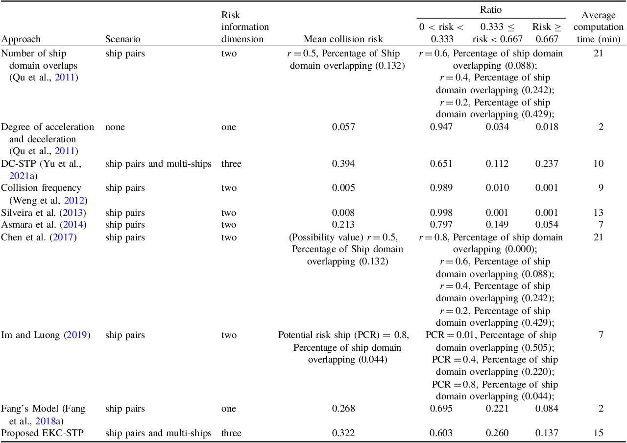
EKC-STP can identify the collision risk for encountering ship pairs and multi-ship crossing scenarios. EKC-STP can reduce the overestimation of interaction possibility from non-considerations of the depth of water in EKC-STP without constraints of the depth of water-based method, the direction changes, and maximum acceleration and velocity bound of encountering ships in O-CSTP, and the static obstacles and speed loss as well as of the depth of water in DC-STP. EKC-STP can make up for the shortfall that it is very hard to define the reliable ship domain for encountering ship pairs in various confined waters, as shown in Table 1. Qu et al. (Reference Qu, Meng and Suyi2011), Chen et al. (Reference Chen, Mou and van Gelder2017) and Im and Luong (Reference Im and Luong2019) all use potential risk ship domain to determine risk criteria, but the definition of ship domain is the same as Qu et al. (Reference Qu, Meng and Suyi2011) and Chen et al. (Reference Chen, Mou and van Gelder2017), and different from Im and Luong (Reference Im and Luong2019). However, the ship domain size for encountering ship pairs in various confined waters is hard to accurately determine. EKC-STP has the advantage of identifying high-risk situations compared with the risk calculated by the degree of acceleration and deceleration. Weng et al. (Reference Weng, Meng and Qu2012) and Silveira et al. (Reference Silveira, Teixeira and Soares2013) used the collision probability multiplying collision candidates to characterise the collision risk, which confronts the challenge of identifying the high-risk encountering scenarios because the collision probability may be incorrect and incomplete. EKC-STP enables for assessment of multi-ship collision risk in confined water, not just for ship-pairs encountering by the (Fang et al., Reference Fang, Yu, Ke, Shaw and Peng2018a) model and head-on crossing in fairways by Asmara et al. (Reference Asmara, Kobayashi, Artana, Masroeri and Wakabayashi2014).
In comparison with O-CSTP-based method and EKC-STP without constraints of the depth of the water-based method, the EKC-STP-based method can reduce the overestimation of interaction possibility, for example, 5739 of 7417 scenarios contribute to a total 849.775 overestimation using EKC-STP without constraints of the depth of the water-based method, and all 7417 scenarios having overestimation between 0.00045 and 0.543 using the O-CSTP-based method. As for the O-CSTP-based method, the overestimation depends on the direction changes and maximum acceleration and velocity bound of encountering ships. Ordinarily, sailing ships cannot instantly change their course at will and they often gradually change sailing direction under acceleration. Thus, constraints on the sailing direction cannot be ignored in analysing the interaction possibility. In comparison with DC-STP, the mean risk for all scenarios including ship pairs and multi-ships encountering scenarios are smaller derived from EKC-STP. Furthermore, the ratio for risk larger than 0.333 calculated by DC-STP is larger than that obtained from EKC-STP, and overestimation is more evident in the scenarios with risk higher than 0.667. On the one hand, the overestimations of DC-STP are from the static obstacles and speed loss when the ships change directions. Ship navigation is not only limited by built-up area, main farm, other facilities, obstruction, etc., but also by water depth, especially for the ship with large draughts. This kind of ship often enters the port through deep water lanes because it will easily cause grounding without sufficient depth of lanes. Therefore, the depth of water should be taken into consideration for evaluating the interaction possibility for encountering ships. For the 1638 scenarios, all the potential areas have enough water depth for encountering ships, so the interaction possibilities calculated by the EKC-STP without or with constraints of the depth of the water-based method are the same.
In comparison with the AIS-based approach proposed by (Fang et al., Reference Fang, Yu, Ke, Shaw and Peng2018a), the proposed EKC-STP-based method has the capability of identifying the possible interactions for multiple encountering ships to avoid a collision in ports, as shown in Figure 5. The mean, maximum and total interaction possibility for 850 scenarios with multi-ship collision avoidance are 0.379, 0.929 and 322.150, respectively. The proposed method can also identify 6907 of 7757 scenarios with ship-pairs collision avoidance, of which mean, maximum and total interaction possibility are 0.254, 0.998 and 1754.378, respectively. The correlation coefficient between the interaction possibilities derived from the EKC-STP-based method and near-miss risks for ship-pairs scenarios is 0.661, which demonstrates the possible interaction possibility has a strong relationship with the near-miss collision risk for encountering ships, and the interaction probability to some extent can reflect the encountering ships’ near-miss collision risk. The EKC-STP-based method and Fang’s model have the same baseline that high speed, high direction changes and close distance cause big near-miss risks and high interaction possibility. The models proposed by Qu et al. (Reference Qu, Meng and Suyi2011) and Chen et al. (Reference Chen, Mou and van Gelder2017) are both based on the overlapping of fuzzy quaternion ship domains for crossing ship pairs, in which it can easily be observed that the bigger the possibility value (r) that describes the values of radii to define the boundary of the domains, the smaller the probability of risk. This is consistent with the changes of ratios for 0 < risk < 0.333, 0.333 ≤ risk < 0.667, risk ≥ 0.667 calculated by EKC-STP. The higher the risk, the smaller the possibility. Im and Luong (Reference Im and Luong2019) have proposed a potential risk ship domain to characterise the danger of encountering ship pairs, in which 0.8 ≤ potential collision risk (PCR) < 1 means a very dangerous zone, 0.4 ≤ PCR < 0.8 is the dangerous zone, 0.01 ≤ PCR < 0.4 represents cautious zone and 0 < PCR < 0.01 is the safe zone. This indicates the domain zones decrease as the PCR increases. The percentages for safe zone, cautious zone and dangerous zone overlapping are 0.505, 0.220 and 0.044, respectively. This demonstrates that there are no more than 0.044, 0.220 and 0.505 percentages of encountering ship-pairs that appear very dangerous, dangerous and cautious domain invasions. The proposed EKC-STP-based method has identified highly probable collision, likely to collide and low collision risk accounted for 0.137, 0.260 and 0.603, respectively. The differences between the high and low risk calculated by the EKC-STP-based method and Im and Luong (Reference Im and Luong2019) may be related to the ignorance of multi-ships encountering scenarios in the model of Im and Luong (Reference Im and Luong2019). Weng et al. (Reference Weng, Meng and Qu2012) and Silveira et al. (Reference Silveira, Teixeira and Soares2013) both have taken the collision probability derived from the statistics of the historical incidents into consideration, and their collision risks are equal by multiplying the collision probability and collision candidates. However, these two models make it very hard to identify the dangers encountering ship-pairs since the historical incidents’ statistics may be incorrect and incomplete. Asmara et al. (Reference Asmara, Kobayashi, Artana, Masroeri and Wakabayashi2014) have only considered the head-on scenarios in fairways and cannot evaluate the collision risk for other encounter scenarios.
However, there are also some limitations in computation time and identifying all the encounter ship-pairs, for example, the EKC-STP-based method has more computation time and cannot identify the encounter ship-pairs that have small sailing speed, small direction changes and are relatively far away. The advanced EKC-STP-based method that is less time-consuming and a more optimal solution for identifying all the encounter ships is the future research trend.
Comparative analysis with other methodologies for ship collision risk evaluation in confined waters

4.4. Insights from practical application
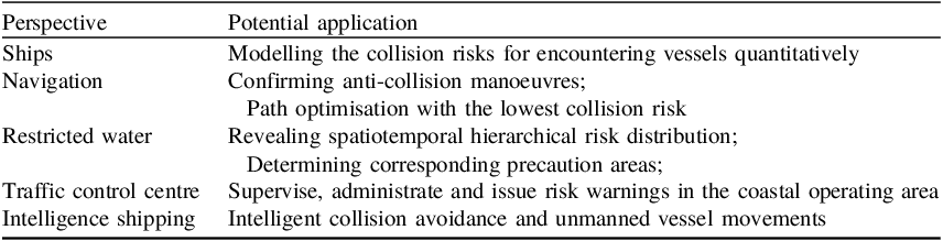
There are some practical applications derived from the interaction probability of multi-ships based on EKC-STP, as shown in Table 2. First, it can intelligently monitor and identify the potential risk quantitatively rather than qualitatively, adaptively predict the collision risks of ship pairs and multiple encountering vessels, and apply to the embedded on-board system and equipment for navigation and avoid the collision because of more consistency with decision making in restricted waters. Second, the collision risk estimation is applicable in ship navigation and path optimisation derived from the lowest collision risk, confirming anti-collision manoeuvres conforming to real-time traffic environment conditions. The travel context of a specific region can be obtained through geographical information including land, shallows, buildings areas, single buildings, maricultural zones and depth of water. The dynamic information for ship information including latitude, longitude, velocity and course at each timestamp can be derived from the real-time AIS information. The risk can be timely estimated based on the sequential possible ship locations calculated based on the ship’s manoeuvrability, ship dynamic navigation information and travel context. The assessed collision risk offers forewarning to take the corresponding precautions and alleviate measures to strengthen vessel operation safety. Third, the risk map obtained from the proposed EKC-STP-based approach could be a valuable prior knowledge base for navigators and other participators in maritime transportation and safe management. The known beforehand high-risk region can support individual ships to pay more attention to the dangerous situation and take timely collision-avoidance manoeuvres to avoid collisions based on the risk estimated from the EKC-STP model. The EKC-STP-based model can also be useful for other interested personnel, including the base station, navigation centre, administration office and vessel traffic service (VTS) centre, to supervise, administrate and issue risk warnings for vessels in the coastal jurisdictional water areas. Finally, space–time-sensitive collision risk prediction can be used in intelligent collision avoidance and unmanned vessel movements employing real-time online collision avoidance decision and control using the distributed decision-making system and modern communication techniques. All in all, it provides theoretical and practical guidance and valuable insight for the decision-making process of ship collision prevention, maritime safety management and risk control options selection.
Insights from practical application

5. Conclusion and prospects
Assessing and estimating the potential ship collision risk is crucial in the navigation industry, maritime transportation, safety management and marine resources protection. This paper proposed an EKC-STP-based approach to quantify the interaction possibility of encountering vessels to estimate the collision risk. This approach provides an innovative method to identify where, when and how often ships probably have interacted and been able to uncover spatiotemporal collision risk patterns over a day and night period. Such an experiment was performed using a long-term data set with numerous individual ships; the results could support understanding how interaction patterns change over space and time and perhaps give insights into the social management of the ships. The findings demonstrate that merely considering the direction constraints removing the static obstacles or considering the depth of water bound from unconstrained spatiotemporal prisms will cause a significant overestimation of an individual vessel’s potential travel area and interaction possibility of encountering vessels in restricted water areas. The proposed EKC-STP-based method enables identifying the possible interactions of multi-ship collision avoidance in ports rather than only for ship-pair scenarios. Most areas in Xiamen Port did not differ remarkably in terms of the total risk in different periods of a day based on the whole month dataset, but some locations have a significant difference in the daily mean collision risk and also have temporal heterogeneity. This means some areas with continuous high risk need to be paid more attention at all times, and some areas need to pay more notice at a specific time, such as day or night.
Some aspects could be explored in future research. First, the EKC-STP-based method could be further extended by taking the ship size and type into consideration, and proposing the composite space–time prism to deal with the different interaction possibilities for different ships. Second, assessing the factors (e.g. climate conditions, traffic density, geographical environment and surrounding traffic flow) affecting vessel collision risk and severity is beneficial for decision-makers in early warning and for proposing efficient guidance and strategies to minimise the likelihood of high-damage collision accidents. Third, the implementation of the proposed method and analysed results could be further enhanced by designing practical software embedded in the collision risk control system, navigation decision-making system, route planning system and maritime authority management system. The interactive interface between the collision risk map and navigating behaviour could greatly facilitate the widespread use of the proposed method. Finally, the quality of the AIS data, for example B-class systems with resolution equal to or lower than 30 s, can be further enhanced through multi-source data fusion analysis, including SAR (Synthetic Aperture Radar), LiDAR (Light Detection and Ranging), HRRP (High-Resolution Range Profile), optical remote sensing image and photographic images.
Funding statement
This work was supported by the National Natural Science Foundation of China (No. 42101429 and No. 42371415); Open Fund of State Key Laboratory of Information Engineering in Surveying, Mapping and Remote Sensing, Wuhan University (Grant No. 21S04), the National Key Research and Development Program of China (No. 2022YFC3302703), and the Young Elite Scientists Sponsorship Program by China Association for Science and Technology (CAST) (No. YESS20220491).
Competing interests
The authors declare that they have no known competing financial interests or personal relationships that could have appeared to influence the work reported in this paper.