1. Introduction
Turbulent gravity currents are produced when a finite volume of dense fluid is rapidly released from a source above a horizontal boundary into an environment of lower density. The dense fluid propagates horizontally under gravity along the lower boundary of the flow domain by displacing the original fluid in place. Owing to the considerable importance of gravity currents in many geophysical and environmental flows, their dynamics have been studied in some detail, using a combination of laboratory experiments and mathematical models. Important applications have been described by many authors (Simpson Reference Simpson1997) and, amongst other phenomena, include: the dynamics of cold fronts; the spread of dense gas following release from a vessel, for example in an explosion; the dynamics of submarine turbidites, which are dilute particle-laden flows (Buckee & Kneller Reference Buckee and Kneller2000); and volcanic ash flows (Sparks et al. Reference Sparks, Bursik, Carey, Gilbert, Glase, Sigurdsson and Woods1997). In the context of many of the above flows, the propagation speed and the density structure of the flow as it spreads from the source are of considerable interest. The key advance in this work is a quantitative assessment of the dilution of a two-dimensional gravity current by mixing of the fluid originally ahead of the current and displaced by the current: to this end, we combine new laboratory experiments with a new theoretical model.
1.1. Historical perspective
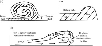
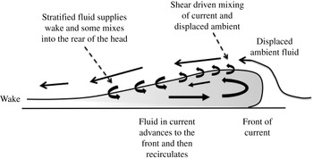
One of the first analyses of the dynamics of a gravity current was presented by von Karman (Reference von Karman1940), in which the critical role of the head of the flow was recognised, and in which potential theory was used to predict that the front of the current makes an angle of 60° with the ground. In this analysis, mixing between the fluid in the head and the ambient was neglected. However, subsequently, Prandtl (Reference Prandtl1952), in discussing the advance of a mass of cold air along the ground, proposed that there would be mixing between the head of the cold current and the ambient fluid, and this led him to infer that the speed of the fluid in the current would exceed the speed of the head (figure 1 a). This work stimulated many measurements in the atmosphere (e.g. Berson Reference Berson1958) which suggested that the speed of the front was in the range 0.5–0.65 times the speed of the fluid supplying the cold front.
Schematic of the flow profile and mixing process in the head envisaged by (a) Prandtl; (b) Hallworth et al. (Reference Hallworth, Huppert, Phillips and Sparks1996); (c) the present work, building from Kneller, Bennett & McCaffrey (Reference Kneller, Bennett and McCaffrey1999).

Meanwhile, in a highly influential paper, Brooke-Benjamin (Reference Brooke-Benjamin1968) introduced a two-layer model for the dynamics of a two-dimensional gravity current and the ambient fluid through which it propagates, using an integral approach to describe the conservation of momentum flux across the head of the flow. This model diverged from the picture proposed by Prandtl, in that there was no account of the mixing or recirculation in the head of the flow, and the fluid speed was assumed to equal the speed of the flow front (figure 1
b). Many studies have built from the pioneering contribution of Benjamin, focusing on modelling the location of the head of the current as a function of time. For currents which remain of high Reynolds number sufficiently far from the source, it has been shown that there is an initial near-source phase of constant speed, followed by a phase of slowly waning speed (Hoult Reference Hoult1972; Chen Reference Chen1980; Huppert & Simpson Reference Huppert and Simpson1980; Rottman & Simpson Reference Rottman and Simpson1983; Bonnecaze, Huppert & Lister Reference Bonnecaze, Huppert and Lister1993; Marino, Thomas & Linden Reference Marino, Thomas and Linden2005). Rottman & Simpson (Reference Rottman and Simpson1983) suggested that, during the initial phase of constant speed, a bore propagates from the back of the gravity current, eventually catching the front of the flow; they developed a two-layer shallow-water model, neglecting any effects of mixing and presented some experiments to illustrate the phenomenon. In the experiments, a shadowgraph identified a region of strong stratification at the rear of the head, which propagated towards the front of the current, and this was described as the bore. In the subsequent waning phase, experimental data have shown that the front of the gravity current follows a power-law distance–time relationship of the form
 $x_{n}(t)\sim {\it\lambda}B^{1/3}t^{2/3}$
where
 $B$
is the total buoyancy, given by the product of the volume of fluid behind the lock gate and the reduced gravity of this fluid per unit width of the two-dimensional channel, and
 $t$
is the time after release of the fluid, while
 ${\it\lambda}$
is a constant. These observations have led to a series of models for the flow, based on shallow-water theory of a single- or two-layer flow (Hoult Reference Hoult1972; Chen Reference Chen1980; Bonnecaze et al.
Reference Bonnecaze, Huppert and Lister1993). The models have been shown to admit self-similar solutions in which it is assumed that there is no mixing, so that the volume of the current is constant. As a result, the solutions predict that the depth of the flow decreases as the lateral extent of the flow increases, while the buoyancy of the current remains a constant. In these models, it has been assumed that at the front of flow the fluid speed equals the speed of advance of the current,
 $u=\text{d}x_{n}/\text{d}t$
, and that the speed of the fluid is given by
 $u=Fr(g^{\prime }h)^{1/2}$
where
 $Fr$
is the Froude number, and
 $g^{\prime }h$
is the product of the reduced gravity,
 $g^{\prime }$
, and the depth of the flow,
 $h$
, at the front.
However, following the early work of Prandtl (Reference Prandtl1952), there have been several key experiments which demonstrate that the fluid in a gravity current mixes with the ambient fluid, leading to considerable dilution and an increase in the volume of the flow (Hallworth et al.
Reference Hallworth, Huppert, Phillips and Sparks1993, Reference Hallworth, Huppert, Phillips and Sparks1996; Hacker, Linden & Dalziel Reference Hacker, Linden and Dalziel1996; Marino et al.
Reference Marino, Thomas and Linden2005). Hacker et al. (Reference Hacker, Linden and Dalziel1996), and later Marino et al. (Reference Marino, Thomas and Linden2005), used a light attenuation technique to measure the dilution of the flow, and presented some fascinating data which illustrate that the flow develops a complex stratified structure as it mixes with the ambient fluid. Marino et al. (Reference Marino, Thomas and Linden2005) focused on measuring the effective local Froude number for the speed of the flow front, based on experimental measurements of both
 $g^{\prime }$
and
 $h$
near the front of the flow. Hallworth et al. (Reference Hallworth, Huppert, Phillips and Sparks1993, Reference Hallworth, Huppert, Phillips and Sparks1996) used a pH indicator, together with an acid and base in the current and ambient fluid, to measure the mixing in the head of the current. By varying the initial pH of the current and ambient fluids in successive, otherwise identical experiments, they were able to produce estimates of the degree of mixing in the head of the flow as a function of the distance from the source. Based on their data, they proposed that some of the ambient fluid ahead of the current is mixed into the head, and that, in turn, the head then emits some of the mixed fluid to form a wake. Hallworth et al. (Reference Hallworth, Huppert, Phillips and Sparks1993, Reference Hallworth, Huppert, Phillips and Sparks1996) then developed an integral model for the volume and buoyancy of the head. The model did not examine the evolution of the wake, but the reduced gravity of the fluid being detrained from the head into the wake is predicted to become progressively smaller as the current advances and the reduced gravity of the head falls. They also reported that the head of the current remains undiluted for some distance from the source, and that only then does it begin to mix and dilute. The transition from a current in which the reduced gravity in the head equals that of the fluid originally behind the lock gate to one in which the reduced gravity of the head progressively decreases with distance from the source was also reported in the data of Marino et al. (Reference Marino, Thomas and Linden2005), with the transition occurring in the region 8–10 lock lengths ahead of the source. In his review paper, Huppert (Reference Huppert2006) discussed the observation of a density-stratified current reported by Hacker et al. (Reference Hacker, Linden and Dalziel1996) and contrasted this with the data of Hallworth et al. (Reference Hallworth, Huppert, Phillips and Sparks1993, Reference Hallworth, Huppert, Phillips and Sparks1996), inferring that the processes of mixing and dilution remain an unresolved feature of gravity current dynamics. To help interpret controls on the mixing in the near-source region, Fragoso, Patterson & Wettlaufer (Reference Fragoso, Patterson and Wettlaufer2013) quantified the evolution of the available potential energy of the current (Winters et al.
Reference Winters, Lombard, RiIey and D’Asaro1995) and other researchers have carried out very high resolution numerical simulations (Hartel, Meiburg & Necker Reference Hartel, Meiburg and Necker2000).
Following a different approach, McElwaine (Reference McElwaine2005) has developed some new solutions, using potential theory, for an idealised non-mixing gravity current, building on the classical work of von Karman (Reference von Karman1940) and Yih (Reference Yih1966). He predicts that there is a vortex with anticlockwise circulation in the head of a flow propagating to the right. This has some qualitative similarities with measurements of the velocity within gravity currents. For example, Thomas, Dalziel & Marino (Reference Thomas, Dalziel and Marino2003) presented some particle image velocimetry measurements which reveal a circulation near the top of the head of the current, but also a second circulation near the base of the current. Kneller et al. (Reference Kneller, Bennett and McCaffrey1999) also presented data on the vertical velocity profile in a gravity current, which identified that there is a significant vertical shear in the flow, with a velocity maximum in the lower half of the current and a velocity reversal near the top of the flow. As well as measurements of the velocity profile, observations of the head of a gravity current include descriptions of cleft and lobe structures (Simpson & Britter Reference Simpson and Britter1979; Simpson Reference Simpson1997) which lead to the engulfment of ambient fluid and are associated with the detailed process of mixing in the head region of the current. This mixing provides a critical connection between the head and tail of the current.
As mentioned above, there are a range of so-called ‘box models’, and also self-similar solutions of shallow-water theory (e.g. Hoult Reference Hoult1972; Chen Reference Chen1980; Bonnecaze et al. Reference Bonnecaze, Huppert and Lister1993) which have been proposed to describe the motion of gravity currents produced from the release of a finite volume of fluid behind a lock. However, the majority of these neglect the mixing with ambient fluid, but subsequent experimental observations (Hallworth et al. Reference Hallworth, Huppert, Phillips and Sparks1993, Reference Hallworth, Huppert, Phillips and Sparks1996; Marino et al. Reference Marino, Thomas and Linden2005; this paper) have suggested that (i) all fluid in the current has become diluted once the flow has travelled of the order of 7–10 lock lengths and (ii) the volume of the current increases by a factor of 3–4 over the first 8–10 lock lengths (§ 3, figure 9 a). A more recent, purely theoretical model has hypothesised that mixing in a gravity current occurs on the upper surface of the flow, based on the value of the Richardson number on the upper surface of the flow (Johnson & Hogg Reference Johnson and Hogg2013). However, this model predicts that the reduced gravity of the current decreases downstream, in contrast to the experimental data reported in Marino et al. (Reference Marino, Thomas and Linden2005) and herein, for currents which have propagated up to 25 lock lengths downstream of the source. Experimental data show that the reduced gravity has a maximum at the head of the current, and smoothly decreases upstream towards the lock gate. This suggests that, in detail, there is a different process governing the mixing and evolution of density in the flow, at least in a region up to 25 lock lengths beyond the original lock gate.
1.2. Modelling the mixing
In this paper we investigate the process of mixing in a gravity current, focusing on the region up to approximately 25 lock lengths downstream of the source. Using light attenuation techniques, as well as video analysis, we present new experimental data concerning the evolution of the density, speed and depth of our experimental gravity currents as they spread along a flume. We also report a series of new experimental observations of the mixing within the gravity current, in which we use dye as a tracer to illustrate the flow pattern and process of mixing. Building from these observations, we develop a new depth-averaged model for the dynamics of a two-dimensional gravity current, produced from the release of a finite volume of fluid, as it propagates along a flume. We combine our observations with the model to develop some new self-similar solutions for the flow. Following a description of the experimental technique, we have divided the presentation into two parts.
First, we describe the initial adjustment phase of the flow, following the release of a finite volume of fluid of uniform density from behind the lock gate. As the head advances up to the point
 $x_{n}=7L$
, we find that the leading part of the head is composed of original lock gate fluid and has a nearly constant depth, so that it advances with a constant speed. During this phase, we establish that a circulation develops as fluid at the front of the current mixes with some of the ambient fluid displaced by the current. The mixed fluid rises over the head, and supplies a dilute wake behind the flow (figure 1
c). Our dye studies suggest that, during this phase, the original lock gate fluid advances towards the nose of the flow with a speed of approximately 1.35 times the speed of the nose. This is comparable to the speed of the ‘bore’ identified by Rottman & Simpson (Reference Rottman and Simpson1983), and we find that this bore catches the front of the flow in the region
 $7L<x_{n}<8L$
. By measuring the change of volume of the current as a function of time, we also estimate that during this adjustment regime a fraction
 $0.75\pm 0.05$
of the ambient fluid displaced by the advancing current becomes mixed into the current.
In § 4, we explore the dynamics after the initial mixing regime, once the gravity current has become vertically and laterally stratified in density. We find that it rapidly adjusts towards a self-similar regime, in which the recirculating flow continues to supply relatively dense fluid into the head, where it mixes with the ambient fluid displaced by the flow, and then circulates back over the head to feed the tail of the current. In this regime, we show that the position of the head of the current increases with time as
 $x_{n}\sim B^{1/3}t^{2/3}$
, where
 $B$
is the total buoyancy of the current per unit width of the lock gate, and
 $t$
is time. In addition, we find that the reduced gravity of the head scales as
 $g^{\prime }(x_{n})\sim B^{2/3}t^{-2/3}H^{-1}$
, while the depth of the head has near constant value
 $h(x_{n})\approx 0.38H$
, with
 $H$
the total depth of the fluid in the flume. We test this picture by measuring the depth and reduced gravity of the current as it propagates along the flume. We also show experimentally that, at a given time, the reduced gravity increases as we move from the tail into the head of the current.
Motivated by these experimental results, we develop a new class of self-similar solutions for the motion of an idealised gravity current based on the depth-averaged equations for the flow. The novelty of our model is twofold. First, the velocity and reduced gravity of the current are vertically stratified, both being greater in the lower half of the current. As a result, the vertical average of the product of the speed and the reduced gravity exceeds the product of the vertically averaged speed and the vertically averaged reduced gravity. In the laterally stratified flow, this results in the continual transport of the reduced gravity towards the head of the flow, and hence, at a given time, there is a gradual increase in the vertically averaged reduced gravity if one moves downstream through the current, i.e. towards the front of the current from the lock gate. Second, based on our dye studies, and in accord with velocity profiles measured by Kneller et al. (Reference Kneller, Bennett and McCaffrey1999), we model the entrainment and mixing of ambient fluid into the flow as occurring primarily in the head region of the flow. We quantify the rate of entrainment in terms of the fraction
 $E$
of the fluid directly ahead of the current which is mixed into the current as it is displaced by the current. We compare the ensuing self-similar solutions for the shape and structure of the current with our experimental data, and determine the best fit coefficients for the above scaling laws controlling the position and reduced gravity of the head of the flow. Finally we draw some conclusions, and discuss the implications of our results more broadly.
We note at this stage that our work relates to gravity currents released into a two-dimensional flume of finite depth. Our experiments span a range of initial volume and reduced gravity, leading to flows with Reynolds number in the range 3000–40 000 (see later, figure 10
d). This range overlaps with the majority of published experimental data on gravity currents (e.g. Rottman & Simpson Reference Rottman and Simpson1983; Bonnecaze et al.
Reference Bonnecaze, Huppert and Lister1993; Hallworth et al.
Reference Hallworth, Huppert, Phillips and Sparks1993; Marino et al.
Reference Marino, Thomas and Linden2005; Fragoso et al.
Reference Fragoso, Patterson and Wettlaufer2013). We have also explored the dynamics as the aspect ratio of the lock gate ranges from
 $H/L=0.25{-}3.0$
. There is clearly a much broader range of experiments which could be conducted, and in which many other properties are changed. However, the present body of experiments forms a coherent description of the dynamics of a gravity current produced by a finite release of buoyancy into a fluid of finite depth, and in which we account for the displacement and mixing of the ambient fluid originally ahead of the current.
2. Experimental method
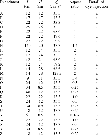
A series of turbulent laboratory gravity currents were generated through the release of a finite volume of aqueous salt solution into a 3 m long Perspex tank of width 15 cm and depth 36 cm. The details of the parameters for each experiment are shown in table 1, including the depth of the fluid,
 $H$
, the length behind the lock gate,
 $L$
, and the aspect ratio
 $AR$
of the source,
 $H/L$
, as well as the reduced gravity associated with the salinity,
 $g_{o}^{\prime }$
. In many of the experiments, the aqueous solution was initially dyed with a known mass of red TRS food dye, and the tank was backlit using a matrix LED light panel (W&Co Displays and Signs). In order to measure the dilution of the current associated with the mixing, solutions with different concentration of dye were placed in the experimental tank, in sequence, and the red–green–blue (RGB) light intensity was recorded for each such solution using a Nikon D90 RGB DSLR camera. The images were analysed using a MATLAB script in order to generate a calibration curve relating light intensity and salinity, averaged along the path of each light ray, following an approach analogous to Hacker et al. (Reference Hacker, Linden and Dalziel1996), Fragoso et al. (Reference Fragoso, Patterson and Wettlaufer2013) and van Sommeren, Caulfield & Woods (Reference van Sommeren, Caulfield and Woods2012). The experimental images can then be analysed to determine the distribution of salt within the tank. The total mass of salt as measured during an experiment typically varied by 2–5 wt%. The camera was set to take between 2 and 4 frames per second with shutter speed
 $1/100$
, aperture F8 and ISO 800. The precise timing of the images was checked carefully in a control experiment. The camera recorded 14 pixels
 $\text{cm}^{-1}$
in the vertical and horizontal directions throughout the flow domain.
3. Adjustment from a homogeneous to a stratified flow
In presenting our experimental results of the initial adjustment, we normalise horizontal distance
 $x$
and vertical distance
 $y$
with the lock length,
 $L$
, leading to dimensionless lengths
 $\hat{x},{\hat{y}}$
, current depth
 ${\hat{h}}$
and time
 $\hat{t}$
defined as
 $$\begin{eqnarray}\hat{x}=\frac{x}{L},\quad {\hat{y}}=\frac{y}{L},\quad {\hat{h}}=\frac{h}{H},\quad \hat{t}=\frac{t}{{\it\tau}},\end{eqnarray}$$
where the time scale
 ${\it\tau}=(L/g_{o}^{\prime })^{1/2}$
, with
 $g_{o}^{\prime }$
the initial reduced gravity of the dense fluid behind the lock gate. The salt concentration
 $C$
is scaled with the initial salt concentration
 $C_{o}$
, leading to the dimensionless salt concentration
 ${\hat{c}}=C/C_{o}$
. Assuming the salt concentration is small, the reduced gravity varies linearly with the salt concentration so that
 $g^{\prime }({\hat{c}})=g_{o}^{\prime }{\hat{c}}$
. In this limit, the concentration of salt and the reduced gravity are directly equivalent.
3.1. Evolution of the reduced gravity, depth and position of the current
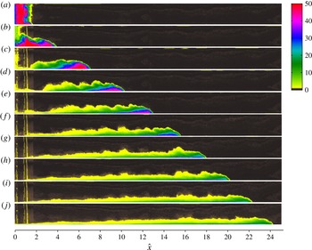
Figure 2(a–j) illustrates the time evolution of the gravity current for experiment I1 (table 1). The false-colour images correspond to the concentration of the fluid in the tank at 10 times after release of the lock gate. The current initially adjusts after removing the lock gate, and as the front, located at position
 $\hat{x}=\hat{x}_{n}(t)$
, advances through the region
 $2<\hat{x}_{n}<7$
, the current has a nearly constant density head region, followed by a growing tail, in which the density decreases with distance behind the front and with height above the base of the current. As the current continues to lay down a dilute tail, the region of near constant density at the front of the flow becomes progressively smaller, and eventually dissipates as it advances beyond the point
 $\hat{x}_{n}=7$
(c,d). As the flow continues, the buoyancy everywhere in the flow becomes progressively smaller with time, with the buoyancy increasing from the lock gate towards the head.
(a–j) Photographs of a saline gravity current illustrating the evolution of the salinity, as shown by false-colour contours, as current I1 (table 1) advances along the flume. Images are taken at equal dimensionless time intervals in each case. The
 $x$
-axis scale shows the position in the current as a function of the number of lock lengths beyond the lock gate (3.1). The colour scale denotes concentration of salt measured in
 $\text{g}~\text{l}^{-1}$
.

Table of experiments illustrating range of aspect ratio and volume. (a) Light attenuation experiment; (b) dye injected into head of the flow; (c) dye injected into the ambient fluid.

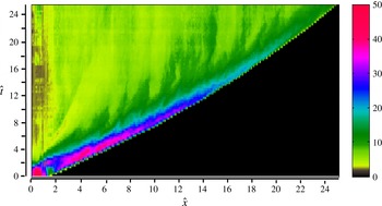
Evolution of the depth-averaged concentration of the current as a function of position and time. The horizontal axis represents position ahead of the lock and the vertical axis is time. The colours represent the depth-averaged salt concentration of the gravity current, with the legend illustrating a linear scale from 0 to
 $50~\text{g}~\text{l}^{-1}$
, where
 $50~\text{g}~\text{l}^{-1}$
corresponds to the concentration of salt in the original fluid behind the lock gate. The figure illustrates how the concentration varies with position and with time in the current and shows that the head of the flow becomes progressively more dilute, with the initial buoyancy in the flow being dispersed from the lock gate up to the head of the flow.

To help visualise the changes in the flow as it advances along the tank, in figure 3 we present a false-colour image of the vertically averaged current concentration as a function of position and time for experiment I1. This image illustrates how the speed of the head is constant up to the point
 $\hat{x}_{n}\approx 7$
, and, in this near lock gate region, the fluid directly behind the front of the current has reduced gravity equal to that of the fluid behind the lock gate. However, downstream of this point, the speed and the reduced gravity of the head gradually decrease with distance. The figure also shows how an ever-growing tail develops in which the concentration gradually increases from the lock gate towards the head of the current. Finally, the figure shows how, at a given position in the tank, behind the head, the concentration gradually decreases with time.
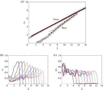
(a) Characteristic diagram illustrating the dimensionless position of the front and rear of the head of the current, as a function of dimensionless time, for experiments A–G, I1 and O–P. The rear is defined as the horizontal position on the fluid surface
 ${\hat{c}}=0.95$
at which the height equals
 $0.3h_{cm}$
, where
 $h_{cm}$
is the depth of the current where the depth-averaged concentration is a maximum (see figure 1). Symbols for the different experiments are: A, red diamonds; B, red triangles; C, blue triangles; D, grey circles; E, purple diamonds; F, grey squares; G, green triangles; I1, blue circles; O, blue squares; P, orange circles. (b) Variation of the vertically averaged dimensionless salt concentration,
 $\overline{c}$
, as a function of the distance along the current. Data are shown at a series of times as the current advances along the tank. In (b), corresponding to experiment C (table 1), the first three profiles have nearly constant concentration at the front of the flow (
 $\hat{x}_{n}<7$
), while in the subsequent profiles, corresponding to more distal positions of the front of the flow, the salt concentration of the head region gradually decreases. (c) Variation of the depth of the current as a function of position in the current for the same experiment as in (b). The data shown in (b,c) are typical of all the experiments.

Using the new data, in figure 4 we show the dimensionless position of the front of the gravity current,
 $\hat{x}_{n}(t)$
, as a function of time, for experiments A–G, I1, and O–P (table 1). The data collapse to a universal curve, labelled ‘front’, independent of aspect ratio, buoyancy and current volume (cf. Huppert & Simpson Reference Huppert and Simpson1980). Our images also show that as we move back into the current from the head, the region of fluid whose reduced gravity equals that of the fluid behind the lock gate initially deepens and then thins out (figure 2). To illustrate how the size of this region evolves in time, we first measure the surface in the fluid where the reduced gravity is a fraction
 $0.95$
of the original reduced gravity of the fluid behind the lock gate. We then find the depth of the current at which the depth-averaged concentration is a maximum, say
 $h_{cm}$
, and we draw a horizontal line at a height
 $0.3h_{cm}$
above the lower boundary. Finally, moving forwards along this line from the origin, we measure the location at which this line first meets the surface on which the reduced gravity equals
 $0.95$
of the original lock gate fluid. Measurements of this location, as a function of time, for experiments A–G, I1 and O–P are plotted in figure 4(a). Again, although there is some scatter, the data seem to collapse to a universal curve, labelled ‘rear’ for
 $\hat{x}_{n}>2$
. We note that, near the origin, several waves of dense fluid may form as the flow slumps from the lock gate to form the current (figure 2
a,b). In this region,
 $\hat{x}_{n}<2$
, depending on the variations from experiment to experiment, the above measurement may select a transient wave behind the main head as corresponding to the rear of the current. However, as the current then self-organises into the familiar head and wake structure, the trailing waves wane and so further from the source,
 $\hat{x}_{n}>2$
, this measurement of the rear surface of the head collapses towards a universal line for all our experiments, as shown with black dashes in figure 4(a). If a higher horizontal line is chosen, we see some scatter in the data owing to the turbulent fluctuations which develop and drive the mixing just behind the point
 $x(h_{cm})$
(see later), and so in the present work we show the intersection of the line
 $y=0.3h_{cm}$
with the contour on which the reduced gravity equals
 $0.95$
of the original value.
We note that in the original work of Rottman & Simpson (Reference Rottman and Simpson1983), data were presented showing the location of the front of the gravity current and of a ‘bore’ which was described as advancing from the back wall of the tank towards the front of the head. This was apparently measured from shadowgraph data. The data in figure 8 of Rottman & Simpson (Reference Rottman and Simpson1983) represent the location of what they described as a ‘bore’. The data very nearly map onto the curve we describe as ‘rear’, although the ‘bore’ tends to spread a little more slowly downstream, perhaps a result of the shadowgraph picking up the density gradient which develops behind the head (figure 2). In summary, we find that, in the dimensionless
 $(\hat{x},\hat{t})$
space, the leading edge follows the relation
 $\hat{x}=(0.45\pm 0.03)\hat{t}+1.4$
while the trailing edge follows the relation
 $\hat{x}=(0.63\pm 0.03)\hat{t}-1.3$
. As these two curves converge, the region between the curves, in which the density equals the original density of the fluid behind the lock gate, dissipates. Subsequently, the fluid everywhere in the current has a smaller density than the original fluid released from the lock (figures 2 and 3).
In figure 4(b) we show how the vertically averaged concentration (or, equivalently, reduced gravity) of the current varies with position in the current. Curves are shown for a series of times as the current advances from the source. The experiment corresponds to a current with initial aspect ratio 1 (experiment C, table 1). For convenience, in this figure, we have defined the vertically averaged concentration as
 $$\begin{eqnarray}\bar{c}=\frac{{\hat{s}}}{{\hat{h}}(\hat{x},\hat{t})},\end{eqnarray}$$
where
 ${\hat{s}}(\hat{x},\hat{t})$
represents the total dimensionless salt content of the current per unit distance along the boundary
 $$\begin{eqnarray}{\hat{s}}(\hat{x},\hat{t})=\int _{0}^{{\hat{h}}(\hat{x},\hat{t})}{\hat{c}}(\hat{x},{\hat{y}})\,\text{d}{\hat{y}}\end{eqnarray}$$
and where
 ${\hat{h}}$
(
 $\hat{x}$
,
 $\hat{t}$
) represents the maximum dimensionless height at which a concentration signal above background noise is detected. In the present experiments,
 ${\hat{h}}(\hat{x},\hat{t})$
is taken to be the height at which the dye concentration falls below
 $4\,\%$
of the initial concentration behind the lock gate. Figure 4(b) illustrates that the dimensionless average concentration in the head of the flow remains approximately constant until
 $\hat{x}_{n}\approx 7$
, beyond which it gradually decreases. Note that the vertically averaged concentration includes the lower part of the current composed of original lock gate fluid, and the upper part of the flow composed of mixed fluid (figure 2).
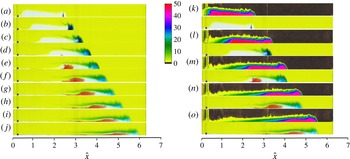
(a–j) Series of photographs illustrating the migration of a point release of blue dye and red dye into a clear gravity current propagating through a yellow environment (experiment Z, table 1). (k–o) Series of false-colour images of the concentration measured in an experiment with identical initial conditions, experiment Q, above the corresponding images of the dye from experiment Z in (a,c,e,g,i), at five different times. This panel is included in order to help calibrate the dye movement, shown in (a–j), relative to the overall structure of the current.

In figure 4(c) we show profiles of the current depth as a function of position within the current, with the profiles taken at times corresponding to the concentration profiles shown in figure 4(b). It is seen that the depth at the nose of the current is approximately uniform in the region
 $2<\hat{x}_{n}<7$
. However, as the head advances further downstream, the depth adjusts to what appears to be another fixed value
 ${\hat{h}}_{n}\sim 0.38$
(see § 4). The combination of constant depth and reduced gravity at the head enables the flow to advance with constant speed in the region
 $2<\hat{x}_{n}<7$
. However, once the flow has become mixed and stratified, the reduced gravity throughout the current gradually decreases and the flow adjusts to the self-similar regime in which the speed also gradually wanes (§ 4). The data shown in (b) and (c) are typical of all our experiments.
3.2. Mixing at the head of the current
In order to build up understanding of how the mixing occurs, we have carried out a series of experiments in which we inject and then track a small volume of dye in both (i) the current and (ii) the ambient fluid. Figure 5 illustrates a gravity current of originally clear fluid advancing into a yellow ambient fluid (experiment Z, table 1). In this experiment, a pulse of blue dye was injected into the current, at the position
 $\hat{x}=2.4$
when the front of the current was at position
 $\hat{x}_{n}=2.6$
. Later a pulse of red dye was injected at the point
 $\hat{x}=2.3$
when the front was at position
 $\hat{x}_{n}=3.7$
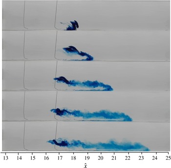
. Panels (a–j), taken at equal dimensionless time intervals, illustrate how the blue and the red dye pulses migrate with time. In figure 5(k–o), we illustrate the density structure in an equivalent current, at five times, as obtained from a second identical experiment, Q. This second series of figures has been included in order to help relate the position of the dye relative to the current. As the flow continues along the flume, the blue dyed fluid catches up with the nose of the current. The front region of the current becomes blue and feeds a rising stream of dyed fluid which passes up over the top of the continuing gravity current. This forms a streak of blue fluid which propagates backwards relative to the nose of the continuing current (b–d). As the current advances the intensity of the blue dye decreases. Also, the red dye, which is initially injected in fluid further upstream in the current, progressively catches up with the front of the current.
Characteristic diagram in which (a) the trajectory of the leading edge of a series of parcels of dye injected within several of the experimental currents are followed in the
 $\hat{x}{-}\hat{t}$
plane. In this panel, the solid and dotted red lines correspond, respectively, to the position of the leading edge of the gravity current and the point at which the contour on which the concentration is 0.95 of the original concentration meets the horizontal line
 $0.3h_{cm}$
. In the insert, for each set of data, the position of the leading edge of the dye has been mapped so that the first point coincides with the origin. The insert shows that all the data collapse onto one curve, suggesting the fluid speed within the head is constant with position and time. Note that, based on our dye measurements, the fluid speed within the head is constant with position and time until
 $\hat{x}\sim 7$
. (b) The trajectories followed by a series of parcels of dye which are injected into the ambient fluid ahead of the current. The dye begins to move backwards as the front of the current arrives, and it continues to move backwards until the rear of the head passes by. The dye then slows down substantially, as the stratified tail of the current passes by. The dotted, dot-dashed and dashed red lines illustrate the points at which the contours where the concentration has value 95 %, 70 % and
 $50\,\%$
of the original concentration in the fluid behind the lock gate meet the line
 $y=0.3h_{cm}$
(cf. figure 4
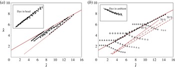
a). These lines gradually diverge as the tail spreads and the current becomes stratified. In (a), data are shown from experiments R–V with the experimental data denoted as: R, circles; S, squares; T, triangles; U, diamonds; and V, stars. In (b), data are shown for experiments W–Z, with data denoted as: W, circles; X, squares; Y, triangles; and Z, diamonds.

In figure 6(a), we have plotted the dimensionless trajectories of the leading edge of a series of dye pulses injected into the currents which formed during different experiments (R–V). In the insert in this figure, we have mapped each set of data so that the initial position of the leading edge of the dye coincides with the origin, (0, 0). It is seen that, to a reasonable approximation, the dye streaks from the different experiments advance with a uniform speed. This suggests that, in these experiments, the dye, and hence some of the fluid within the current, travels at a speed up to
 $1.35\pm 0.05$
times the speed of the front of the current. This is very similar to the speed of the rear of the gravity current head which we presented in figure 4(a). Given the range of volumes and reduced gravities in the experiments which we have carried out, we suggest that this value is representative for high-Reynolds-number gravity currents in a finite depth ambient fluid, as explored herein.
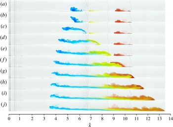
Illustration of the motion of three parcels of dye initially injected upstream of the gravity current near the base of the experimental tank (experiment W, table 1). The parcels of dye were injected at the positions
 $5<\hat{x}<6$
at
 $\hat{t}=9.3$
(blue),
 $7<\hat{x}<8$
at
 $\hat{t}=13.8$
(yellow), and
 $9<\hat{x}<10$
at
 $\hat{t}=18.2$
(red). (a–j) Show the location of the dye at a series of times as the current advances along the tank. The fluid in the gravity current initially has no dye.

On reaching the front of the current, the dyed fluid appears to rise up over the top of the current, mixing with some of the fluid originally ahead of the current, which is also displaced over the current. Once the current has passed by, this feeds the tail of the current. The precise process controlling the mixing may involve the mixing of ambient fluid initially overridden by the flow, and the incorporation of ambient fluid in the lobe and cleft structure of the head (cf. Simpson Reference Simpson1997, Buckee & Kneller Reference Buckee and Kneller2000). There are also eddies which appear to form on the upper surface of the head of the current, in a manner reminiscent of Kelvin–Helmholtz billows, and these lead to the intermingling of the fluid displaced over the head of the flow with fluid from the head. This effective detrainment of original fluid from the head, and its circulation over the head to feed the tail of the flow, rationalises how there is a decrease in the volume of fluid which has the original concentration (figures 2 and 3). The dye dispersal experiments for
 $\hat{x}_{n}>7$
suggest that, as the current becomes stratified, progressively more of the recirculating fluid can mix back into the rear of the head rather than supplying the tail. This leads to the formation of a density-stratified current.
We now turn to the motion of the ambient fluid as the gravity current passes by, since this provides a complementary perspective on the mixing in the head region of the flow. In figure 7 we illustrate the evolution of three regions of dyed ambient fluid originally located ahead of the current (Experiment W, table 1). As the undyed gravity current reaches each of the patches of dyed ambient fluid, it is seen that the ambient fluid rises over the current and mixes with some of the fluid at the front of the current. Panels (a–c) show the mixing of the blue dye, originally located in the region
 $5<\hat{x}<6$
. Owing to the stratification in the wake, there is a weak shear flow which develops, and causes the blue dyed region to shear out in the wake, consistent with the velocity profile measured by Kneller et al. (Reference Kneller, Bennett and McCaffrey1999) (§ 4). Very little blue fluid appears to enter the head region. Panels (d,e) show the evolution of a patch of yellow dye, initially located in the region
 $7<\hat{x}<8$
. After rising over the top of the current, some of this yellow dyed fluid is mixed back into the head, which appears to include an anticlockwise vortex, and the remainder of the yellow fluid is dispersed into the wake. Panels (e–g) illustrate the mixing associated with a red patch of dye, initially located in the region
 $9<\hat{x}<10$
. This mixes in a similar manner to the yellow dye, leading to further dilution of the head and growth of the wake immediately behind the head.
For comparison with the motion of the fluid originally in the current (figure 6
a), in figure 6(b) we show the trajectory of a series of parcels of dye injected into the ambient fluid initially ahead of the current. The leading edge of this dye appears to move backwards as the head passes. In the insert in figure 6(b), for each data set, we have rescaled the time and position so that the dye meets the front of the gravity current head at a rescaled time of
 $0$
and position
 $0$
. We then compare the speed of each dye pulse as it moves backwards towards the origin while the current passes by. The data are somewhat noisy but suggest that, for
 $2<\hat{x}_{n}<7$
, the dye located above the current, at position
 $\hat{x}<\hat{x}_{n}$
, moves upstream with a speed which has a value of approximately
 $0.66\pm 0.05$
times the speed of the front of the current. In the main figure, for comparison, we also show the position of the front of the current (solid red line) and the position where the contours at which the concentration in the current has value 0.95, 0.7 and 0.5 of the original concentration meet the horizontal line
 $y=0.3h_{cm}$
. Figure 8 summarises the flow pattern during this initial mixing regime.
Cartoon illustrating the flow pattern during the initial mixing and dilution of the flow, as the current advances with a constant front speed. Fluid ahead of the current mixes with fluid reaching the front, then rises up over the advancing flow, and feeds the growing stratified tail of the current.

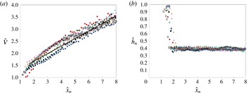
Variation of (a) the volume and (b) the height of the current head as a function of
 $\hat{x}_{n}$
in the region
 $0<\hat{x}_{n}<8$
containing the initial mixing zone, in which the fluid at the front of the current has the buoyancy of the fluid behind the lock gate. As the flow advances, there is a near linear increase in volume while the depth of the flow approaches a near constant value. Data are shown for experiments B–G and O–P, with data displayed with the following symbols: B, crosses; C, solid squares; D, diamonds; E, triangles; F, stars; G, plus; O, circles; P, hollow squares.

3.3. Entrainment coefficient during the mixing of the original lock fluid
We have measured the instantaneous volume of the current and the depth at a distance
 $H/2$
behind the front as a function of the distance travelled by the nose of the current, and this is shown in figure 9(a,b). The figure illustrates that there is some fluctuation in the volume and depth measurement associated, for example, with the time-dependent billow structures on the upper surface of the flow (figure 2). However, an ensemble average over all our experiments leads to the approximate relation that
 $$\begin{eqnarray}\hat{V}=1+(0.31\pm 0.02)\hat{x}_{n},\end{eqnarray}$$
where
 $\hat{V}=\int _{o}^{\hat{x}_{n}}{\hat{h}}(\hat{x})\,\text{d}\hat{x}$
, while the depth of the head of the current tends to a value of approximately
 ${\hat{h}}_{n}={\hat{h}}(x_{n})\approx 0.38\pm 0.04$
after an initial adjustment. We can define the fraction of the ambient fluid directly ahead of the current and which is entrained into the flow,
 $E$
, by the relation
 $$\begin{eqnarray}\frac{\text{d}\hat{V}}{\text{d}\hat{t}}=E{\hat{h}}(x_{n})\frac{\text{d}\hat{x}_{n}}{\text{d}\hat{t}}.\end{eqnarray}$$
Using the values shown in figure 9, (3.5) suggests that during the initial adjustment phase the entrainment coefficient lies in the range
 $0.7<E<0.8$
.
During this initial dilution of the turbulent gravity current the fluid at the flow front has density comparable to the initial value of the current. However, beyond this region the mixing leads to a fully density-stratified flow and a reduction in the buoyancy of all the fluid. The different balance of the flow may then lead to a change in the entrainment coefficient
 $E$
as defined by (3.5). In the following section we aim to determine the entrainment coefficient further downstream as the flow becomes self-similar. Differences in the entrainment rate during this initial adjustment and the subsequent self-similar flow may lead to an effective virtual origin in time of the self-similar flow, as we account for this in the analysis below.
4. The long-time self-similar regime
4.1. Experimental measurements of the head of the flow
We now present a series of measurements of the evolution of the speed of the head, the reduced gravity of the head and the depth of the flow, once the current has advanced beyond the initial mixing region, and become fully stratified. This provides the basis for the development of a new model of gravity current dynamics including a description of the entrainment at the head of the flow.
Numerous papers have proposed that, during this second regime, the position of the flow front should follow the scaling relation, obtained from dimensional arguments,
 $$\begin{eqnarray}x_{n}(t)\sim B^{1/3}(t+t_{o})^{2/3},\end{eqnarray}$$
where we have included a time offset
 $t_{o}$
to accommodate any difference in the rate of dilution of the flow during the initial mixing phase described above. To test the scaling in (4.1) we have calculated the ratio
 $$\begin{eqnarray}X(t)=\frac{x_{n}(t)}{B^{1/3}(t+t_{o})^{2/3}}\end{eqnarray}$$
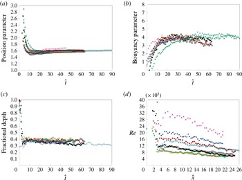
as shown in figure 10(a). After an initial transient,
 $X\rightarrow 1.6\pm 0.05$
. In making the plot, we have estimated a value for
 $t_{o}$
for each experiment to optimise the fit of the model, and, in all cases, this has a value in the range
 $1<t_{o}<2$
s, which is considerably shorter than the 10–30 s typical of the experiments. Since the value
 $t_{o}>0$
, we infer that, in the initial adjustment phase, the mixing is more rapid. The scaling (4.1) is in good accord with earlier measurements of gravity currents (cf. Huppert & Simpson Reference Huppert and Simpson1980, Marino et al.
Reference Marino, Thomas and Linden2005).
Data from experiments H–N (table 1) illustrating (a) the variation of
 $X(t)=x_{n}(t)/B^{1/3}(t+t_{o})^{2/3}$
, the position of the nose of the current as a function of dimensionless time; (b) the variation with dimensionless time of
 $G(t)=\overline{g}_{n}^{\prime }(t+t_{o})^{2/3}H/B^{2/3}$
, where
 $\overline{g}_{n}^{\prime }$
is taken to have the value of the vertically averaged reduced gravity at a distance
 $H/2$
behind the front of the flow; (c) the variation with dimensionless time of the depth of the current at a distance
 $H/2$
behind the front of the flow. We have estimated the best fit value for the virtual release time,
 $t_{o}$
, and this has values in the range 1–2 s for all data shown. (d) Variation of the Reynolds number measured at a distance
 $H/2$
behind the front of the flow, as a function of the dimensionless position of the front of the current,
 $x_{n}/L$
, for each of the experiments shown in (a–c). In each panel, the data from each experiment H–N are denoted by the following symbols: H, plus; I1, solid squares; I2, hollow squares; J, circles; K, triangles; L, diamonds; M, crosses; N, stars.

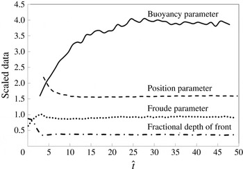
Average of the data from eight different experiments H–N (table 1) illustrating the variation with dimensionless time of the position parameter,
 $X(t)$
(4.1); the buoyancy parameter,
 $G(t)$
(4.2); the fractional depth of the front,
 $h_{n}/H$
; and the Froude number,
 $Fr=(\text{d}x_{n}/\text{d}t)/(\overline{g}_{n}^{\prime }h_{n})^{1/2}$
measured at the point a distance
 $H/2$
behind the front of the flow. It is seen that at long time,
 $X\sim 1.6$
,
 $G\sim 4.0$
,
 $h/H\sim 0.38$
and
 $Fr\sim 0.9$
.

We have measured the depth and concentration of the current at a distance
 $H/2$
behind the front of the current, as a representative value for the head of the flow (figure 10
b,c). The depth data exhibit some fluctuation in value with time and also from experiment to experiment (figure 10
c). If we average over all the experiments, the mean height appears to be approximately constant, with value
 $h/H\sim 0.38\pm 0.04$
, following the initial adjustment of the flow to the self-similar regime (figure 11).
If the depth of the head of the current is approximately constant with time, then the conservation of buoyancy suggests that the reduced gravity should decrease in proportion to the lateral extent of the flow. We therefore expect the reduced gravity at the head of the flow to decrease according to a relation of the form
 $$\begin{eqnarray}\overline{g}_{n}^{\prime }=G(t)B^{2/3}H^{-1}(t+t_{o})^{-2/3},\end{eqnarray}$$
where the dimensionless quantity
 $G(t)$
should tend to a constant following the initial adjustment. Since the current is vertically stratified we work with the depth-averaged buoyancy, and define
 $\overline{g}_{n}^{\prime }=g_{o}^{\prime }\overline{c}_{n}$
where we evaluate the vertically averaged salt concentration at the point
 $H/2$
behind the leading edge of the current. We have tested this scaling by measuring the value of
 $G(t)$
(4.3) as a function of time for the different experiments H–N in table 1 (figure 10
b). It is seen that, although there is some fluctuation, possibly associated with the turbulent fluctuations on the top surface of the flow near the head,
 $G(t)\rightarrow 4.0\pm 0.4$
at long times (figures 10
b and 11).
For each of the experiments shown in figure 10(a–c), the Reynolds number at the head of the flow, given by
 $Re=(h_{n}/{\it\nu})(\text{d}x_{n}/\text{d}t)$
, where
 ${\it\nu}$
is the kinematic viscosity, remained in excess of 4000 (figure 10
d). In other experiments, for which the initial volume of fluid was smaller, we found that once the Reynolds number at the head falls below a value of approximately 2500, the buoyancy of the head begins to decrease to smaller values than given by the scaling law (4.3), and the effects of the no-slip condition and viscous resistance from the base of the tank begin to influence the front of the flow (cf. Huppert & Simpson Reference Huppert and Simpson1980). In this study, we focus on flows with higher Reynolds number, which appear to follow the self-similar scaling law (4.3).
In figure 11, we also show the average value of
 $Fr$
, averaged over all the experiments shown in figure 10, as a function of dimensionless position, where
 $Fr$
is defined by the relation
 $$\begin{eqnarray}\frac{\text{d}x_{n}}{\text{d}t}=Fr(\overline{g}_{n}^{\prime }h_{n})^{1/2}.\end{eqnarray}$$
It is seen that
 $Fr\rightarrow 0.9\pm 0.5$
once the current has passed through the initial adjustment region. This value is comparable to the values measured by Marino et al. (Reference Marino, Thomas and Linden2005).
4.2. Structure of the current
The data presented above illustrate that mixing is central to the evolution of the gravity current; in order to understand the process of the mixing in some detail we have injected dye into the ambient ahead of the current at position
 $\hat{x}=17$
. We then follow the evolution of the dye as shown in the series of photographs in figure 12. It is seen that the dyed fluid rises up over the upper surface of the current as the current continues forwards, and some of the dyed fluid mixes with current fluid, forming a region of intermediate density which extends forwards into the head of the current. These observations suggest that the displaced ambient fluid mixes with the gravity current fuid in the head region of the flow and that, as the mixture of current and ambient fluid rises up over the head, it supplies both the tail and the head of the flow, leading to a vertically and laterally stratified flow.
To explore this further, we have measured the vertical profile of the concentration in the current at a series of points along the current, and at different times, when the current has advanced different distances along the flume. In figure 13(a), we show a series of vertical density profiles taken at points
 $x/x_{n}=0.2,0.4,0.6$
and
 $0.8$
, for currents with
 $x_{n}/L=19.0,21.5$
and
 $24.0$
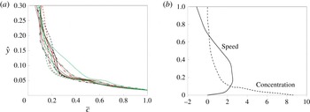
, in which we have normalised each profile relative to the maximum concentration on that profile. This illustrates that there is a significant vertical gradient of concentration, with a relatively dense lower part of the flow, overtopped by a mixed region. These data are consistent with that presented by Altinakar, Graf & Hopfinger (Reference Altinakar, Graf and Hopfinger1996) for a gravity current produced from a maintained source. The structure of this stratification is similar along the length of the current, and also as the current migrates along the flume. In (b), we illustrate the ensemble-averaged vertical buoyancy profile derived from (a), as well as the average velocity profile as reported by Kneller et al. (Reference Kneller, Bennett and McCaffrey1999). In this panel, we have normalised both the buoyancy and the speed so that they both have a mean of unity averaged over the depth of the flow.
Illustration of the mixing of a parcel of dye injected ahead of the current at position
 $\hat{x}=17$
. Panels correspond to pictures taken at equal time intervals. The intense region of blue dye is carried over the head, and some of the blue dye is then stripped from it to form a streak of blue dye which extends forwards from the region of intense dye to the head of the current.

(a) Variation of the concentration as a function of the depth in the flow, as measured at a series of times and at a series of points
 $x/x_{n}=0.2,0.4,0.6,0.8$
as the current advances along the flume. (b) Ensemble-average of the velocity profile from Kneller et al. (Reference Kneller, Bennett and McCaffrey1999) and the concentration profile across the depth of the flow taken from (a), with the data normalised to have a mean of unity over the depth of the flow. In (b), the vertical axis has been normalised so that the depth of the current is unity. In (a), data from experiment I1 are shown at positions
 $x/x_{n}$
given by 0.8, solid; 0.6, dashed; 0.4, dotted; 0.2, dash-dotted and for the times when the nose has position
 $\hat{x}_{n}$
given by 19, green; 21.5, red; 24, black.

We have also measured the variation of the vertical integral of the reduced gravity,
 $\bar{g}^{\prime }h=\int _{0}^{h}{\hat{g}}^{\prime }(x,t)\,\text{d}y$
per unit length of the current, and the vertical extent of the current,
 $h$
, as a function of the position in the current,
 ${\it\eta}=x/x_{n}$
. The vertical integral of the reduced gravity has then been normalised with respect to the expression given in (4.3), leading to the normalised quantity
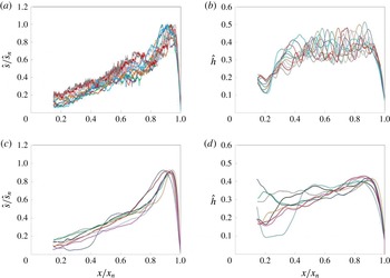
 $\overline{g}^{\prime }(x)h/\overline{g}_{n}^{\prime }h_{n}={\hat{s}}/{\hat{s}}_{n}$
and this is shown as a function of
 $x/x_{n}$
in figure 14(a). In figure 14(b), we show the variation of the depth of the current, normalised by the total depth of fluid in the flume,
 $H$
, as a function of
 $x/x_{n}$
. For a given current, the variation of
 ${\hat{s}}/{\hat{s}}_{n}$
and
 ${\hat{h}}$
with
 $x/x_{n}$
is similar as the current advances from
 $x_{n}=12L$
to
 $x_{n}=21L$
, although there is some scatter owing to the turbulent nature of the flow (cf. figures 2 and 3). We have also calculated the time average of
 ${\hat{s}}/{\hat{s}}_{n}$
and
 ${\hat{h}}$
as a function of
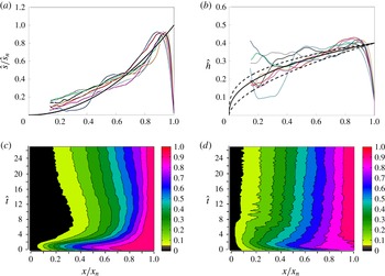
 $x/x_{n}$
for the eight different currents, H–N, and the results are shown in figure 14(c,d). It is seen that, for each of these quantities, the variation with position in the current,
 $x/x_{n}$
, is similar from experiment to experiment, although there is some scatter, perhaps associated with the randomness of the turbulent fluctuations in the flow. We also note that as the current spreads along the flume to distances of the order of 20–25 lock lengths then, in the region of the lock gate, the current becomes very dilute and difficult to resolve accurately. In figure 14, we therefore only present the data in the region
 $0.15<x/x_{n}<1.0$
.
Variation of (a) the dimensionless vertical integral of salt concentration,
 ${\hat{s}}/{\hat{s}}_{n}$
, which is equivalent to
 $\overline{g}^{\prime }h/\overline{g}_{n}^{\prime }h_{n}$
, and (b) the depth,
 ${\hat{h}}$
, of the current, both as a function of the position within the current,
 $x/x_{n}$
for experiment I1. The different coloured curves shown in the plot correspond to those for which the head of the current had dimensionless position
 $x_{n}$
given by: 12, light blue; 13, dark blue; 14, light red; 15, green; 16, purple; 17, turquoise; 18, orange; 19, blue–grey; 20, pink; 21, dark red; 22, grey. (c,d) Time-averaged structure of
 ${\hat{s}}/{\hat{s}}_{n}$
and
 ${\hat{h}}$
as a function of the position,
 ${\it\eta}=x/x_{n}$
, in the current, obtained by time averaging over 20 profiles from the time when
 $x_{n}=12$
to that when
 $x_{n}=24$
. Curves are shown corresponding to data collected from experiments H–N, as indicated by the colours: H, orange; I1, solid black; I2, dotted black; J, red; K, green; L, dark blue; M, purple; N, light blue.

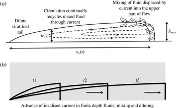
The data shown in figure 14 suggest that in the far field, as the influence of the initial conditions becomes less important and the current becomes fully stratified, then the depth and vertical integral of the buoyancy adjust to a particular profile along the length of the flow. A circulation develops, with the denser fluid in the current being supplied to the front of the current from the lower part of the flow where the speed is a maximum (cf. Altinakar et al. Reference Altinakar, Graf and Hopfinger1996; Kneller et al. Reference Kneller, Bennett and McCaffrey1999; Thomas et al. Reference Thomas, Dalziel and Marino2003, figure 13). This fluid, along with ambient fluid ahead of the current, rises over the top of the head, mixes and feeds the rear of the head and the tail of the flow with fluid of intermediate density (figures 1 c and 15). Since the reduced gravity of the fluid in the lower part of the flow exceeds that higher in the flow (figure 13), we expect the vertical integral of the flux of reduced gravity to exceed the product of the vertically averaged velocity and the vertical integral of the reduced gravity at any point in the flow. As a result, surfaces of constant buoyancy travel faster than the mean flow speed and this may lead to the salinity being a maximum at the front of the current. Furthermore, the scalings for the evolution of the speed and buoyancy at the head of the current, combined with the details of the stratification in the flow, suggest that the flow is self-similar, with the mixing being a key part of the evolution. In the next section, we present a depth-averaged model of the flow based on these ideas, and the assumption that the entrainment of the ambient fluid occurs in the head region of the flow, as the fluid is displaced by the oncoming current, although there is subsequent mixing of this fluid into the oncoming current fluid as the mixture circulates back over the head of the flow.
4.3. The depth-averaged model
In the data described earlier (figure 10), there are fluctuations associated with the turbulent motion, with typical eddy-turnover time
 $h/u$
, where
 $h$
and
 $u$
are the depth and velocity scales of the flow. We are interested in the slow evolution of the flow relative to the local eddy-turnover time, so we describe the motion in terms of the velocity, depth and buoyancy averaged over a time which is long compared to the eddy-turnover time, in an analogous fashion to models of a turbulent buoyant plume (cf. Morton, Taylor & Turner Reference Morton, Taylor and Turner1956). We compare the model predictions with the long-time evolution of the flow once the current extends over length scales much larger than
 $h$
; at this stage the motion is dominantly parallel to the lower boundary, except in the vicinity of the front of the flow.
Schematic of the along-current flow and circulation sketched in the right-hand side. In this regime, self-similar solutions arise with the salinity being carried further forwards.

Applying the Boussinesq approximation and assuming the mixing occurs in the head of the flow (3.5), the local equations for the conservation of mass, momentum and buoyancy, have the form
 $$\begin{eqnarray}\displaystyle & \displaystyle \boldsymbol{{\rm\nabla}}\boldsymbol{\cdot }\boldsymbol{u}=0 & \displaystyle\end{eqnarray}$$
 $$\begin{eqnarray}\displaystyle & \displaystyle {\it\rho}\frac{\partial \boldsymbol{u}}{\partial t}+{\it\rho}\boldsymbol{u}\boldsymbol{\cdot }\boldsymbol{{\rm\nabla}}\boldsymbol{u}=-\boldsymbol{{\rm\nabla}}p+{\it\rho}\boldsymbol{g} & \displaystyle\end{eqnarray}$$
 $$\begin{eqnarray}\displaystyle & \displaystyle \frac{\partial g^{\prime }}{\partial t}+\boldsymbol{u}\boldsymbol{\cdot }\boldsymbol{{\rm\nabla}}g^{\prime }=0. & \displaystyle\end{eqnarray}$$
 $h$
, and use the fact that on the upper surface of the current
 $$\begin{eqnarray}\frac{\partial h}{\partial t}+u(h)\frac{\partial h}{\partial x}=v(h)\end{eqnarray}$$
then we obtain
 $$\begin{eqnarray}\frac{\partial h}{\partial t}+\frac{\partial (h\bar{u})}{\partial x}=0.\end{eqnarray}$$
We now integrate the momentum equation across the depth of the flow,
 $h$
. We use the fact that, for a long thin current, the vertical pressure gradient is hydrostatic,
 $$\begin{eqnarray}p(x,y,t)=p_{o}(x,t)+\int _{y}^{H}{\it\rho}_{o}g\,\text{d}y^{\prime }+\int _{y}^{h}{\it\rho}_{o}g^{\prime }\,\text{d}y^{\prime },\end{eqnarray}$$
where
 $p_{o}(x,t)$
is the ambient pressure along a horizontal surface of height
 $H\,({>}\,h)$
above the lower boundary,
 ${\it\rho}_{o}$
is the ambient density, and
 $g^{\prime }=g({\it\rho}-{\it\rho}_{o})/{\it\rho}_{o}$
. This leads to the result
 $$\begin{eqnarray}\int _{o}^{h}{\it\rho}\frac{\partial u}{\partial t}\,\text{d}y+\int _{0}^{h}{\it\rho}\left(u\frac{\partial u}{\partial x}+v\frac{\partial u}{\partial y}\right)\,\text{d}y=-\int _{0}^{h}\frac{\partial }{\partial x}\left[\int _{y}^{h}{\it\rho}_{o}g^{\prime }\,\text{d}y^{\prime }\right]\,\text{d}y-h\frac{\partial p_{o}}{\partial x}\end{eqnarray}$$
and, combining this with the continuity equation (4.5a ) and the boundary condition (4.6), we can express this equation in the form (Gill Reference Gill1981)
 $$\begin{eqnarray}\frac{\partial (h\bar{u})}{\partial t}+{\it\beta}\frac{\partial \left(h\bar{u}^{2}\right)}{\partial x}=-{\it\gamma}\frac{\partial (h^{2}\bar{g}^{\prime })}{\partial x}-\frac{h}{{\it\rho}_{o}}\frac{\partial p_{o}}{\partial x}.\end{eqnarray}$$
Finally, we can integrate the equation for conservation of buoyancy across the depth of the flow and, combining this with the continuity (4.5a ) and the boundary condition (4.7), we find
 $$\begin{eqnarray}\frac{\partial (h\bar{g}^{\prime })}{\partial t}+{\it\alpha}\frac{\partial (h\bar{g}^{\prime }\bar{u})}{\partial x}=0,\end{eqnarray}$$
where
 $$\begin{eqnarray}h\bar{u}=\int _{0}^{h}u\,\text{d}y,\quad {\it\beta}h\bar{u}^{2}=\int _{o}^{h}u^{2}\,\text{d}y,\quad h\bar{g}^{\prime }=\int _{0}^{h}g^{\prime }\,\text{d}y\end{eqnarray}$$
 $$\begin{eqnarray}{\it\alpha}h\bar{g}^{\prime }\bar{u}=\int _{0}^{h}ug^{\prime }\,\text{d}y\quad \text{and }\quad {\it\gamma}h^{2}\bar{g}^{\prime }(x,t)=\int _{0}^{h}\int _{y}^{h}g^{\prime }(x,y,t)\,\text{d}y^{\prime }\,\text{d}y.\end{eqnarray}$$
The coefficients
 ${\it\alpha}$
,
 ${\it\beta}$
and
 ${\it\gamma}$
(4.13) arise from the vertical distribution of
 $u$
and
 $g^{\prime }$
in the flow, which is stratified in density and velocity (figure 13) and relate to the advection speed of reduced gravity and momentum relative to the vertically averaged flow speed. In the case that
 ${\it\alpha}>1$
the advection speed of the depth-averaged reduced gravity is greater than the depth-averaged fluid speed, and this would result in the total mass of salt per unit length along the current being greatest at the front of the flow. This is in accord with our observations (figure 14) and we return to this observation below.
In this model, we assume the incorporation of the ambient fluid occurs in the head region of the flow; the strong circulation in the head of the flow causes a mixture of ambient and current fluid to rise up and flow back relative to the advancing front. As it rises up, the current fluid and ambient fluid mix, thereby producing a region of intense mixing on the top surface of the current in the neighbourhood of the front of the flow, over a region of lateral extent comparable to the depth of the flow (figures 12 and 15). This mixed fluid then becomes incorporated into the tail and in part the head of the flow. The vertically stratified structure of the wake and the observations of the motion of streaks of dye suggest there is little mixing of ambient fluid directly into the wake further back from the head, above the main part of the current. We seek solutions to the model equations (4.7), (4.10), (4.11) once the current has adjusted towards the apparently self-similar form, at which point the mixing region at the front of the flow is a relatively small part of the flow; therefore, as an approximation, we consider the mixing to occur at the front of the flow. We note that in our model we assume the shape factors for the vertical structure of the current are independent of position in the current. This simplification may not capture the full details of the structure of the flow in and near the head region of the flow where the mixing occurs.
In the model, we have neglected basal friction, since the Reynolds number at the head of the flow remains greater than 4000 (figure 10 d) and, in this case, we find that, to good approximation, the experimental properties at the head of the flow follow the self-similar scalings (figures 10 and 11 a–c). However, friction will eventually become important (Huppert & Simpson Reference Huppert and Simpson1980; Hogg & Woods Reference Hogg and Woods2001).
Equations (4.7), (4.10), (4.11) are to be solved with appropriate boundary conditions at the head of the flow, and subject to the constraint that a finite mass of buoyancy,
 $B$
, was released from the origin,
 $x=0$
. The volume of the current is given by
 $$\begin{eqnarray}V=\int _{o}^{x_{n}}h(x,t)\,\text{d}x.\end{eqnarray}$$
Using (4.7), we also observe that
 $$\begin{eqnarray}\int _{0}^{x_{n}}\frac{\partial h}{\partial t}\,\text{d}x=-\int _{0}^{x_{n}}\frac{\partial \bar{u}h}{\partial x}\,\text{d}x=-\bar{u}(x_{n})h(x_{n}).\end{eqnarray}$$
Hence the evolution of the current volume follows a law of the form
 $$\begin{eqnarray}\frac{\text{d}V}{\text{d}t}=h(x_{n})\left(\frac{\text{d}x_{n}}{\text{d}t}-\bar{u}(x_{n})\right).\end{eqnarray}$$
As in (3.5), we define the entrainment coefficient as the fraction of the ambient fluid displaced by the flow which is mixed into the flow. This is given by
 $$\begin{eqnarray}\frac{\text{d}V}{\text{d}t}=Eh(x_{n})\frac{\text{d}x_{n}}{\text{d}t}\quad \text{and so}\quad \bar{u}(x_{n})=(1-E)\frac{\text{d}x_{n}}{\text{d}t}.\end{eqnarray}$$
We now assume
 $E$
is constant in the self-similar flow regime, and our task is to determine
 $E$
from the experimental data. It is worth remarking that (4.16) requires that the depth-averaged speed of the flow at the front is smaller than the rate of advance of the current. This is possible since the vertical shear in the horizontal velocity profile leads to some of the current fluid travelling faster than the vertically averaged speed; it is this fluid which recirculates over the head of the flow and mixes with the ambient fluid displaced from ahead of the current.
Conservation of buoyancy requires that
 $$\begin{eqnarray}\int _{0}^{x_{n}}h(x,t)\bar{g}^{\prime }(x,t)\,\text{d}x=B.\end{eqnarray}$$
By comparing the terms in (4.10), we expect that, for a self-similar flow, the speed at the nose of the flow is given in terms of the Froude number
 $Fr$
, where
 $$\begin{eqnarray}\frac{\text{d}x_{n}}{\text{d}t}=Fr(\overline{g}_{n}^{\prime }h)^{1/2}.\end{eqnarray}$$
This relation is also consistent with the direct measurement from the experiments (figure 11) which suggests that the value of
 $Fr$
, measured at the point a distance
 $H/2$
behind the front, tends to a constant with value
 $Fr\rightarrow 0.9\pm 0.05$
downstream of the initial adjustment region (§ 3).
4.4. Self-similar solutions
We now seek general self-similar solutions for this model system. In this context, we note that if the fluid has total depth
 $H$
and the current has total buoyancy
 $B$
, then the parameter
 $$\begin{eqnarray}P=\frac{Bt^{2}}{H^{3}}\end{eqnarray}$$
is dimensionless, and so in principle the flow may depend on this parameter. However, guided by the experimental observations of the properties at the front of the current (figures 10 and 11), we seek solutions of the form
 $$\begin{eqnarray}h(x,t)=HP^{a}\mathscr{H}({\it\eta}),\quad \bar{g}^{\prime }(x,t)=\frac{B^{2/3}}{t^{2/3}H}P^{b}\mathscr{G}({\it\eta}),\quad \bar{u}(x,t)=B^{1/3}t^{-1/3}P^{c}\mathscr{U}({\it\eta}),\end{eqnarray}$$
where
 ${\it\eta}=x/x_{n}(t)$
and
 $x_{n}(t)={\it\lambda}B^{1/3}t^{2/3}P^{d}$
. Although we have included the possible dependence on
 $P$
to make the derivation general, given the experimental observations (figures 10 and 11), we expect the appropriate self-similar solutions not to depend on
 $P$
(see below).
If we substitute the ansatz (4.21) into the depth-averaged equations, and apply the boundary conditions, we can find the exponents
 $a,b,c$
and
 $d$
and the shape functions
 $\mathscr{H}$
,
 $\mathscr{U}$
and
 $\mathscr{G}$
. The conservation of buoyancy in the current (4.18) requires that the exponents satisfy
 $$\begin{eqnarray}a+b+d=0\end{eqnarray}$$
while the Froude number condition at the head of the flow requires that
 $$\begin{eqnarray}2c=a+b.\end{eqnarray}$$
Finally, we require that the speed of the flow at the nose,
 $\bar{u}(x_{n},t)$
, is proportional to the rate of advance of the nose,
 $\text{d}x_{n}/\text{d}t$
, and so
 $c=d$
. Combining these three relations requires that
 $$\begin{eqnarray}c=d=0\quad \text{and}\quad a=-b.\end{eqnarray}$$
In the special case of a finite depth of fluid, for a self-similar solution, we expect the depth of the head of the flow to be a constant fraction of the depth of the fluid layer, so that, near the head, the flow in the ambient fluid which is displaced by the current, but not entrained, is also self-similar; this additional condition suggests that
 $a=b=0$
. This is consistent with our measurements (figure 10
b). These arguments suggest that the solution (4.21) is independent of
 $P$
, as suggested by the data (figure 11).
We deduce that
 $$\begin{eqnarray}x_{n}(t)={\it\lambda}B^{1/3}t^{2/3},\end{eqnarray}$$
where
 ${\it\lambda}$
is a constant. Also, by substitution of (4.21) into the conservation equations (4.7) and (4.11), we find the ordinary differential equations governing the variation of reduced gravity, depth and speed
 $$\begin{eqnarray}\left(-\frac{2{\it\lambda}{\it\eta}}{3}+\mathscr{U}\right)\frac{\text{d}\mathscr{H}}{\text{d}{\it\eta}}=-\mathscr{H}\frac{\text{d}\mathscr{U}}{\text{d}{\it\eta}}\end{eqnarray}$$
 $$\begin{eqnarray}-\frac{2{\it\lambda}{\it\eta}}{3}\frac{\text{d}}{\text{d}{\it\eta}}\left(\mathscr{G}\mathscr{H}\right)+{\it\alpha}\frac{\text{d}\mathscr{G}\mathscr{H}\mathscr{U}}{\text{d}{\it\eta}}=0.\end{eqnarray}$$
For such a self-similar solution, we then expect the pressure
 $p(x,t)$
to follow a scaling of the form
 $p(x,t)={\it\rho}_{o}B^{2/3}t^{-2/3}\mathscr{F}({\it\eta})$
, where
 ${\it\rho}_{o}$
is a reference density, so that on substitution into (4.10) we obtain
 $$\begin{eqnarray}-\frac{{\it\lambda}}{3}\mathscr{U}\mathscr{H}+-\frac{2{\it\lambda}{\it\eta}}{3}\frac{\text{d}\mathscr{H}\mathscr{U}}{\text{d}{\it\eta}}+{\it\beta}\frac{\text{d}\mathscr{H}\mathscr{U}^{2}}{\text{d}{\it\eta}}=-\frac{\text{d}\mathscr{H}^{2}\mathscr{G}}{\text{d}{\it\eta}}+\mathscr{H}\frac{\text{d}\mathscr{F}}{\text{d}{\it\eta}}.\end{eqnarray}$$
As a simple ansatz motivated by the profiles in figure 14, if we assume the velocity, reduced gravity and depth are given by power laws of
 ${\it\eta}$
, then (4.27) requires
 $$\begin{eqnarray}\mathscr{U}=\frac{4{\it\lambda}{\it\eta}}{9{\it\alpha}},\end{eqnarray}$$
where we have equated the exponent of
 ${\it\eta}$
on the left-hand side with the first term on the right-hand side of (4.28) to infer that
 $$\begin{eqnarray}\mathscr{H}\mathscr{G}=\mathscr{H}_{\mathit{o}}\mathscr{G}_{\mathit{o}}{\it\eta}^{2}.\end{eqnarray}$$
Equation (4.26) then requires
 $$\begin{eqnarray}\mathscr{H}=\mathscr{H}_{\mathit{o}}{\it\eta}^{2/(3{\it\alpha}-2)}\end{eqnarray}$$
and so
 $$\begin{eqnarray}\mathscr{G}=\mathscr{G}_{\mathit{o}}{\it\eta}^{6(({\it\alpha}-1)/(3{\it\alpha}-2))},\end{eqnarray}$$
where
 $\mathscr{H}_{\mathit{o}}$
and
 $\mathscr{G}_{\mathit{o}}$
are constants. We see from the solution (4.31a
) that, providing
 ${\it\alpha}>1$
, then in this self-similar flow regime, the depth and the reduced gravity increase towards the front of the flow, in accord with the experimental data (figure 14). Note that the pressure term, which arises in (4.28), can also be evaluated from the model given the solution for the speed, depth and reduced gravity.
Using the solution, (4.17) suggests that the fraction of the displaced fluid which is entrained into the current is given by
 $$\begin{eqnarray}E=1-\frac{2}{3{\it\alpha}}.\end{eqnarray}$$
Also, the conservation of total buoyancy (4.18) requires that
 $$\begin{eqnarray}\mathscr{H}_{\mathit{o}}\mathscr{G}_{\mathit{o}}=\frac{3}{{\it\lambda}}.\end{eqnarray}$$
Substituting the solutions into the Froude number condition (4.19), and combining with (4.33), we then find that
 $$\begin{eqnarray}Fr=2\left(\frac{{\it\lambda}}{3}\right)^{3/2}.\end{eqnarray}$$
According to this solution, the fraction of the displaced fluid mixed into the current,
 $E$
, and also the shape of the current,
 $\mathscr{H}({\it\eta})$
, are controlled by the parameter
 ${\it\alpha}$
, while, independently, the conservation of buoyancy and the Froude number impose constraints on
 ${\it\lambda}$
,
 $\mathscr{G}_{\mathit{o}}$
and
 $\mathscr{H}_{\mathit{o}}$
. We now compare the model with our experimental results.
4.5. Mixing during self-similar regime
In order to predict the mixing rate, we need to estimate the value of
 ${\it\alpha}$
(4.32). To this end, we compare the variation of the depth of the flow as a function of position in the current as predicted by the model with the experimental data (figure 14
d). We have taken the time average of the current depth for the eight different experiments shown in figure 14(d), and in figure 16(b) we compare these with the theoretical model (4.31a
) using the values
 ${\it\alpha}=1.8,2.3$
and
 $2.8$
.
Variation of (a) the vertical integral of the salt concentration, normalised by the vertical integral of the salt concentration at the nose,
 ${\hat{s}}/{\hat{s}}_{n}$
, which is equivalent to
 $\overline{g}^{\prime }h/\overline{g}_{n}^{\prime }h_{n}$
, as a function of position in the current,
 $x/x_{n}$
, for the eight experiments H–N. For comparison the model solution (4.30) is also shown with the thick black curve, rescaled to have value unity at
 ${\it\eta}=1$
to be consistent with the dimensionless data. (b) Time average of the depth of the current as a function of the position within the current (cf. figure 14), again compared to the theoretical model prediction (4.31a
) for the dimensionless current depth using the values
 ${\it\alpha}=1.8,2.3$
and
 $2.8$
. Data collected from experiments H–N are indicated by the colours: H, orange; I1, solid black; I2, dotted black; J, red; K, green; L, dark blue; M, purple; N, light blue. Thick lines correspond to the idealised similarity solution. In (c) we present a colour image in which we compare the fraction of the total buoyancy of the current in the region of the current between the rear of the lock gate and each point in the current, as a function of the dimensionless position in the current (
 $x$
-axis) and dimensionless time (
 $y$
-axis). The colour corresponds to this fraction as indicated on the legend, and contours corresponding to fractional values
 $0.1,0.2,\ldots ,0.9$
are also shown on the figure. In (d) we show a colour image of the fraction of the total volume of the current in the region of the current between the rear of the lock gate and each position in the current, as a function of the dimensionless position (
 $x$
-axis) and dimensionless time (
 $y$
-axis). We also include contours of constant volume fraction
 $0.1,\ldots ,0.9$
in the figure.

In comparing the model with the experimental measurements of the depth profile, we note there is some significant scatter in the data, with local differences between the model and the concentration data being as large as 50 % near the transition from the head to the tail. We suggest that some of this results from the turbulent nature of the flow, which leads to variations from experiment to experiment, but there is some systematic difference, especially in the depth-averaged buoyancy just behind the head. It may be that the vertical structure of the current does in fact vary along the current, and especially in the region of the head, whereas for simplicity we have assumed that this is constant in our model, but assessment of this is beyond the scope of our measurements. Nonetheless, the model seems to provide a reasonable leading-order description of the overall behaviour of the flow, if not the local buoyancy just behind the head, and we find that for values of
 ${\it\alpha}$
in the range 1.8–2.8, the absolute fractional difference between the area of the theoretical model (4.31a
) and the average of the eight experimental profiles shown in figure figure 14(d), say
 $h_{a}({\it\eta})$
, as defined by
 $$\begin{eqnarray}\text{err}_{h}=\frac{\displaystyle \int _{0}^{1}|h_{a}({\it\eta})-\mathscr{H}_{\mathit{o}}{\it\eta}^{2/(3{\it\alpha}-2)}|\,\text{d}{\it\eta}}{\displaystyle \int _{0}^{1}\mathscr{H}_{\mathit{o}}{\it\eta}^{2/(3{\it\alpha}-2)}\,\text{d}{\it\eta}}\end{eqnarray}$$
is less than 10 %. This range of values of
 ${\it\alpha}$
corresponds to values of
 $E$
in the range 0.63–0.76.
As an independent check on the value of
 $E$
, we can estimate
 ${\it\alpha}$
from the vertical profile for the speed and reduced gravity of the flow (4.13). Using the data presented in Kneller et al. (Reference Kneller, Bennett and McCaffrey1999) for the speed and the present experiments for the reduced gravity (figure 13), we can apply (4.13) to estimate
 ${\it\alpha}$
. Accounting for the uncertainty in the measurement of concentration in the upper part of the flow, where the flow is quite dilute and where the velocity is negative, leads to an estimate for
 ${\it\alpha}=1.9\pm 0.3$
.
The two different measurements for
 ${\it\alpha}$
overlap in the range
 $1.8<{\it\alpha}<2.2$
and, for this range, (4.32) suggests that
 $E$
, the fraction of the fluid displaced by the head which mixes into the current, has a value in the range
 $0.63<E<0.7$
. This is smaller than our estimate for the entrainment coefficient during the initial adjustment phase of the flow. The difference is consistent with there being a positive value of
 $t_{o}$
, the correction to time in the self-similar solutions (figure 10); the enhanced mixing during the initial slumping phase is equivalent to the current being released earlier. Going forward we use the range
 $0.63<E<0.76$
, consistent with the estimate from our data, (4.35).
4.6. Model parameters
The experimental measurements of the buoyancy and depth at a point
 $H/2$
behind the front of the flow suggest that
 $\mathscr{H}_{0}=0.38\pm 0.04$
while
 $\mathscr{G}_{0}=4.0\pm 0.4$
(figure 10
b,c) so that
 $\mathscr{G}_{0}\mathscr{H}_{0}\approx 1.52$
. However, from figure 10(a), we estimate that
 ${\it\lambda}=1.6\pm 0.05$
. The conservation of buoyancy, (4.33) suggests that
 $3/\mathscr{H}_{0}\mathscr{G}_{0}={\it\lambda}$
. Taking the range of values for
 $\mathscr{H}_{0}$
and
 $\mathscr{G}_{0}$
, we find that the data suggest
 $3/\mathscr{H}_{0}\mathscr{G}_{0}=2.0\pm 0.4$
. Although the lower bound of this range coincides with the value of
 ${\it\lambda}$
obtained from (4.1) and figure 10(a),
 ${\it\lambda}=1.6$
, there is a suggestion that an additional process is affecting the experiments.
Also, using the value
 ${\it\lambda}\approx 1.6\pm 0.05$
(figure 10
a), and combining with (4.34), we predict that the effective Froude number in this stratified flow is
 $Fr\approx 0.79\pm 0.03$
. The actual measurement of the Froude number at a distance
 $H/2$
behind the front, based on the actual depth integral of the reduced gravity and the speed of the flow, is
 $0.9\pm 0.05$
(figure 11). The model prediction is within approximately 12 % of the measurements, but again there is a suggestion of some difference between the model and the data.
In order to investigate this further, in figure 16(a), we compare the normalised experimental data (figure 14
c) with the model prediction, (4.30), for the variation of the vertical integral of the reduced gravity, normalised by the value at the nose,
 $\overline{g}^{\prime }h/\overline{g}_{n}^{\prime }h_{n}$
, as a function of
 ${\it\eta}$
. Note, the theoretical model is scaled by
 $\mathscr{G}_{0}\mathscr{H}_{0}$
, so that the scaled value is one at
 ${\it\eta}=1$
, consistent with the normalised experimental data. Although the general trend in the experimental data is similar to the model prediction, there appears to be a systematic difference between the data and the model in the tail of the flow, where the measured vertical integral of reduced gravity is larger than the model prediction. This difference suggests that some of the saline solution released from behind the lock gate becomes detached from the front of the gravity-driven flow. Given that the speed at the rear of the flow near the lock gate is much smaller than that near the front of the flow, it is likely that the no-slip condition near the base of the tank leads to a finite, but small, part of the flow near the source becoming detached from the ongoing current. Provided that this loss of buoyancy occurs relatively slowly compared to the rate of advance of the flow, we expect that, following the initial adjustment of the flow, the current will evolve approximately according to the self-similar dynamics, but that it gradually evolves from pure self-similar behaviour as progressively more buoyancy is lost at the rear of the flow. In the experiments, the self-similar regime of the flow seems to apply approximately in the region
 $12<x_{n}<22$
(figure 10), where the properties of the head follow the scaling laws (4.1) and (4.3). In the initial slumping phase of the flow, a small part of the source fluid in the tail of the flow may become detached from the continuing head in this lower boundary layer. There may then be a slowly increasing mass of fluid which becomes detached from the rear of the current as it spreads, dilutes and slows. We therefore interpret the measurements of
 ${\it\lambda}$
and
 $\mathscr{G}_{0}$
as relating to the average of the effective buoyancy in the current over the interval
 $12<x_{n}<22$
. In order to estimate this active or effective buoyancy driving the current, we now carry out a very simple approximate analysis. We assume that, in the region
 $12<x_{n}<22$
, the active current only sees a fraction
 $f$
of the total buoyancy released from behind the lock gate. Equations (4.1) and (4.3) would then imply that, based on this reduced buoyancy in the current,
 ${\it\lambda}=(1.6\pm 0.05)/f^{1/3}$
while
 $\mathscr{G}_{0}=(4.0\pm 0.4)/f^{2/3}$
. Conservation of buoyancy (4.33) would then suggest that
 $f=0.8$
, in order that
 ${\it\lambda}\mathscr{G}_{\mathit{o}}\mathscr{H}_{0}=3$
and so the best fit values are
 ${\it\lambda}=1.7$
and
 $\mathscr{G}_{0}=4.6$
to two significant figures. Using this larger value for
 ${\it\lambda}$
, we predict, from (4.34), that the Froude number of the flow is
 $0.87\pm 0.04$
, which is also much closer to the experimental observations. Given the agreement with the speed, the reduced gravity at the front of the flow, the conservation of total buoyancy and the Froude number at the front of the flow, we propose that these revised values correspond to those which would apply to a very high Reynolds number inertial current in which the no-slip boundary effects are very small. It is worth noting that the integral of the absolute difference between the model prediction for the vertical integral of the salinity in the current and the average of the experimental data for the eight experiments shown in figure 16(a), as a fraction of the total salinity in the current,
 $$\begin{eqnarray}\text{err}_{s}=\frac{\displaystyle \int _{0}^{1}|{\hat{s}}({\it\eta})-{\it\eta}^{2}|\,\text{d}{\it\eta}}{\displaystyle \int _{0}^{1}{\it\eta}^{2}\,\text{d}{\it\eta}}\end{eqnarray}$$
is approximately
 $16\,\%$
, which is similar to the fraction of the buoyancy which has been estimated to be left in a boundary region in the tail of the flow,
 $1-f=0.2$
. Since all of the currents have a similar initial volume in our experiments, we expect that the value of
 $f$
is also similar from experiment to experiment. Unfortunately, we could not experimentally test the dependence of
 $f$
over a much larger range in initial volume since, with much smaller initial volume, the Reynolds number of the flow becomes too small for the front of the flow to remain in the inertial regime, while our experimental system is too small to admit significantly larger source volumes.
In order to demonstrate this slow loss of buoyancy from the rear of the current, in figure 16(c) we present a colour image in which we compare the fraction of the total buoyancy of the current in the region of the current between the rear of the lock gate and each point in the current, as a function of the dimensionless position in the current (
 $x$
-axis) and dimensionless time (
 $y$
-axis). The colour corresponds to this fraction as indicated on the legend, and contours corresponding to fractional values
 $0.1,0.2,\ldots ,0.9$
are also shown on the figure. It is seen that, gradually, the dimensionless position of each contour representing a constant fraction of the buoyancy migrates backwards in the current. This redistribution of the buoyancy is consistent with a slow loss of buoyancy from the rear of the current. Our earlier estimate, that the effective buoyancy driving the leading part of the flow in the region
 $12<\hat{x}_{n}<22$
is approximately a fraction 0.8 of the total buoyancy, is consistent with the contours in figure 16(c).
For comparison, in figure 16(d) we show a colour image of the fraction of the total volume of the current in the region of the current between the rear of the lock gate and each position in the current, as a function of the dimensionless position (
 $x$
-axis) and dimensionless time (
 $y$
-axis). We also include contours of constant volume fraction
 $0.1,\ldots ,0.9$
in the figure. The image shows that, in the region
 $x_{n}>10$
, after the current has adjusted, then to good approximation the volume contours are independent of the dimensionless position of the current. This suggests that even though there is a slow loss of buoyancy from the dense lower part of the flow, the current shape remains approximately the same as the current advances. Together, these figures show that strictly the flow is not self-similar owing to the slow redistribution of buoyancy from the front to the rear of the flow. However, this redistribution of buoyancy is a slow process and so the self-similar depth-averaged model seems to provide a reasonable approximate description of the overall dynamics of the gravity current following the initial transition of the flow (§ 3). The details of the entrainment and mixing at the front of the flow have been parameterised by the mixing coefficient
 $E$
, which suggests a fraction in the range
 $0.63{-}0.76$
of the fluid displaced by the current is mixed into the current. We also suggest that in our experiments approximately 20 % of the initial buoyancy of the flow becomes detached from the main advancing flow in a boundary region near the base of the tank in the tail of the flow. In future work, amongst other challenges, it would be of interest to explore the details of the circulation at the front of the flow in more detail and also to quantify the controls on the slow redistribution of buoyancy seen in figure 16(c).
5. Discussion
We have presented a new suite of experiments in which we measure the mixing throughout a gravity current produced by the release of a finite mass of dense fluid from behind a lock gate. During the initial motion, the unmixed dense fluid within the head of the current advances at a speed of the order of
 $(1.35\pm 0.05)u_{n}$
, where
 $u_{n}$
, the speed of the front of the current, has value
 $u_{n}=(0.9\pm 0.05)(g^{\prime }h)^{1/2}$
. As a result, unmixed current fluid arrives at the front of the flow, rises up over the continuing flow and slows down, migrating backwards relative to the front. The recirculating fluid mixes with approximately
 $0.75\pm 0.05$
of the ambient fluid, originally downstream of the current, which is also displaced upwards and backwards by the current. The mixture is then supplied to the tail behind the advancing flow. The trailing edge of the region of original unmixed fluid in the head, which coincides with the ‘bore’ observed by Rottman & Simpson (Reference Rottman and Simpson1983), catches the front of the flow when the front has travelled to a point approximately seven lock lengths downstream,
 $\hat{x}_{n}=7$
(figure 2). As the current advances beyond this point, the circulation and mixing persist and there is a progressive decrease in the maximum density of the head (figures 3 and 4). The current becomes laterally and vertically stratified, with the reduced gravity increasing towards the head.
The continuing flow gradually adjusts to a self-similar profile in which a fraction in the range 0.63–0.7 of the fluid displaced by the current mixes into the current. This mixing appears to occur largely in the head region of the flow and, with the circulation, leads to formation of a substantial vertical and lateral stratification in the current. As the flow advances, the depth of the head remains nearly constant, while the buoyancy of the front of the flow decreases inversely with the position of the nose downstream. This leads to a near linear increase in the volume of the current as the nose advances downstream. Our data are consistent with the classical self-similar result that the position of the nose,
 $x_{n}(t)=1.7B^{1/3}t^{2/3}$
, and the data suggest that the effective Froude number of the head of the flow is approximately
 $0.9\pm 0.05$
. However, in this self-similar regime, we find that the mixing of ambient fluid into the flow causes the vertically averaged reduced gravity at the head of the flow to decrease according to the relation
 $\overline{g}_{n}^{\prime }=4.6B^{2/3}H^{-1}t^{-2/3}$
. We develop a new self-similar model, derived from the depth-averaged equations, by assuming that the mixing with the displaced ambient fluid occurs in the head of the flow. The predictions of this model are in reasonable accord with the measured profiles of the depth-averaged reduced gravity and the depth of the flow. A key element of the model is that, owing to the stratification, the depth-averaged advection speed of the reduced gravity exceeds the depth-averaged speed of the fluid, and so the reduced gravity is maximal at the front of the flow and gradually decreases upstream in the tail. Our data do show however, that there is a slow redistribution of buoyancy from the front and towards the tail of the flow, and so strictly the experimental flows are not self-similar.
The mixing process we have described has numerous implications for density-driven flows in nature and the environment, and we plan to explore these in forthcoming work. We are also presently exploring the implications of the mixing of ambient fluid into the current, as described herein, in the different context of a maintained source of buoyancy and also in an axisymmetric geometry (Samasiri & Woods Reference Samasiri and Woods2015). In both cases the detailed dynamics controlling the value of the entrainment parameter
 $E$
are different, and we plan to report on these studies in the near future.
Acknowledgements
We are grateful for the helpful comments of the referees and for the support of BP in funding this work.