

1 Introduction
Vortex rings are fascinating objects and their study has been pursued for many years (see, for example, Shariff & Leonard Reference Shariff and Leonard1992; Barenghi & Donnelly Reference Barenghi and Donnelly2009). In a typical laboratory setting they are often generated mechanically, that is, a piston ejects, through an orifice, a relatively small amount of fluid into a reservoir, with the piston velocity  $U_{p}$ and the stroke length
 $L$ as the main control parameters. Vortex rings are then formed in the vicinity of the orifice, for certain values of
 $U_{p}$ and
 $L$, and propagate away from it, interacting with the surrounding fluid. A suitable Reynolds number, defined as
 $$\begin{eqnarray}Re=\frac{U_{p}L}{2\unicode[STIX]{x1D708}}=\frac{\unicode[STIX]{x1D6E4}_{0}}{\unicode[STIX]{x1D708}},\end{eqnarray}$$
where  $\unicode[STIX]{x1D708}$ indicates the fluid kinematic viscosity and
 $\unicode[STIX]{x1D6E4}_{0}=U_{p}L/2$ denotes the ring circulation according to the slug flow model, can be used to distinguish between laminar and turbulent rings, although the influence of the orifice geometry and of the piston velocity time history on the resulting ring features cannot be neglected, as discussed, for example, by Glezer (Reference Glezer1988).
Vortex rings can also be generated thermally, that is, by a short heat pulse, when the superfluid phase of liquid 4He (He II) is employed as the working fluid (Stamm et al. Reference Stamm, Bielert, Fiszdon and Piechna1994a,Reference Stamm, Bielert, Fiszdon and Piechnab). He II is obtained by cooling the normal (viscous) phase of liquid 4He (He I) below the transition temperature  $T_{\unicode[STIX]{x1D706}}$ – equal to approximately 2.17 K at the saturated vapour pressure – and is characterized by unique physical properties, such as an extremely large thermal conductivity, which actually depends on the heat flux, and an extremely small kinematic viscosity (see, for example, Barenghi, Skrbek & Sreenivasan Reference Barenghi, Skrbek and Sreenivasan2014; Mongiovì, Jou & Sciacca Reference Mongiovì, Jou and Sciacca2018).
Phenomenologically, the large-scale behaviour of superfluid 4He can be described by the two-fluid model, which postulates the existence of two components. While the superfluid component does not carry viscosity or entropy, the normal component, representing the gas of thermal excitations, behaves as a viscous fluid. Although the density of He II,  $\unicode[STIX]{x1D70C}=\unicode[STIX]{x1D70C}_{n}+\unicode[STIX]{x1D70C}_{s}\approx 145~\text{kg}~\text{m}^{-3}$, is almost temperature independent, strong temperature dependencies are observed for
 $\unicode[STIX]{x1D70C}_{n}$ and
 $\unicode[STIX]{x1D70C}_{s}$, the densities of the normal and superfluid components, respectively. At temperatures very close to
 $T_{\unicode[STIX]{x1D706}}$, He II is entirely made of the normal component and, for temperatures below 1 K, it can be said that only the superfluid component remains.
The velocity field of the superfluid component can be disrupted by one-dimensional topological defects called quantized vortices. Their core has atomic size, that is, of the order of 0.1 nm, and the superfluid component is set into motion around it, ensuring that the circulation around each vortex is equal to the quantum of circulation  $\unicode[STIX]{x1D705}=h/m_{4}=9.97\times 10^{-8}~\text{m}^{2}~\text{s}^{-1}$, where
 $h$ denotes the Planck constant and
 $m_{4}$ indicates the mass of the 4He atom. Typically, the vortices arrange themselves in a tangle and provide the coupling between the two fluid components, as their cores act as scattering centres for thermal excitations, represented by the normal component. It then follows that the flow of one component influences that of the other only when quantized vortices are present – for example, at large enough flow velocities – and quantum turbulence is the name usually given to the phenomenon happening when the quantized vortex tangle enables the mutual interaction between the two components of the fluid.
The thermal generation of vortex rings discussed here occurs in the two-fluid regime of superfluid 4He, that is, above 1 K, and is based on releasing a short heat pulse into a circular tube that opens to the quiescent He II bath, in a way similar to previous studies (Stamm et al. Reference Stamm, Bielert, Fiszdon and Piechna1994a,Reference Stamm, Bielert, Fiszdon and Piechnab). According to the two-fluid model, heat is transported only by the bulk motion of the normal component, which flows away from the heater, and, in the case of steady flow in a channel, the velocity  $u_{n}$ of the normal component is given by
 $$\begin{eqnarray}u_{n}=\frac{q}{\unicode[STIX]{x1D70C}sT},\end{eqnarray}$$
where  $q$ is the applied heat flux,
 $s$ denotes the entropy per unit mass and
 $T$ indicates the temperature; see, e.g. Van Sciver (Reference Van Sciver2012) for details on the derivation of (1.2). At the same time, the superfluid component flows in the opposite direction with a velocity
 $u_{s}$ in order to satisfy the condition of null mass flow rate, i.e. it is assumed that
 $\unicode[STIX]{x1D70C}_{n}u_{n}+\unicode[STIX]{x1D70C}_{s}u_{s}=0$. We can therefore establish an analogy between the piston velocity
 $U_{p}$ and
 $u_{n}$, and the piston stroke length
 $L$ and
 $u_{n}t_{q}$, where
 $t_{q}$ is the duration of the heat pulse (Stamm et al. Reference Stamm, Bielert, Fiszdon and Piechna1994a). It follows that the Reynolds number introduced above, equation (1.1), can be rewritten in our case as
 $$\begin{eqnarray}Re=\frac{\unicode[STIX]{x1D70C}U_{p}L}{2\unicode[STIX]{x1D707}_{n}}=\frac{\unicode[STIX]{x1D70C}u_{n}^{2}t_{q}}{2\unicode[STIX]{x1D707}_{n}}=\frac{\unicode[STIX]{x1D70C}\unicode[STIX]{x1D6E4}_{0}}{\unicode[STIX]{x1D707}_{n}},\end{eqnarray}$$
where the dynamic viscosity  $\unicode[STIX]{x1D707}_{n}$ of the normal component of the fluid is tabulated, e.g. by Donnelly & Barenghi (Reference Donnelly and Barenghi1998).
The just mentioned works (Stamm et al. Reference Stamm, Bielert, Fiszdon and Piechna1994a,Reference Stamm, Bielert, Fiszdon and Piechnab) were motivated by previous experimental investigations on the occurrence of macroscopic vortex rings in He II, generated by using the classical piston–cylinder arrangement and studied by acoustic means (Borner, Schmeling & Schmidt Reference Borner, Schmeling and Schmidt1983; Borner & Schmidt Reference Borner, Schmidt, Meier and Obermeier1985) or by visualization (Murakami, Hanada & Yamazaki Reference Murakami, Hanada and Yamazaki1987). These works on mechanically generated rings also motivated Wacks, Baggaley & Barenghi (Reference Wacks, Baggaley and Barenghi2014) to perform relevant numerical simulations. The main outcome of these studies – see especially the neat experimental results by Borner & Schmidt (Reference Borner, Schmidt, Meier and Obermeier1985) – is that, in the range of investigated parameters, the normal and superfluid components seem to be tightly coupled, in such a way that the generated rings appear to display some classical-like features, regardless of the ring generation mechanism.
It is believed that, at the orifice edges, the normal component of He II behaves as a classical viscous fluid, that is, under certain conditions, a vortex ring is being generated. Then, due to the presence of quantized vortices, the superfluid component is forced to follow the classical behaviour of the normal component, which is driven by the flow geometry. Consequently, once the ring is fully formed, it can be said that the two components move together, in the same direction, and the means used to initiate the fluid motion does not seem to be relevant anymore because the flow geometry is changed significantly at the orifice edges.
We specifically use here (1.3) to characterize the vortex rings thermally generated in superfluid 4He, that is, as a starting point for the comparison of their features to those of other macroscopic vortex rings, both in viscous fluids and in He II. Our scientific aim was to clarify if significant differences could be observed at sufficiently large scales, that is, at scales larger than the mean distance between quantized vortices. As detailed below, it appears that, in the range of investigated parameters, such differences are absent. The work belongs to the active line of scientific research focusing on the study of large-scale quantum features of He II, which have yet to be fully understood, at least from a Lagrangian view point, as discussed, for example, by Švančara & La Mantia (Reference Švančara and La Mantia2017, Reference Švančara and La Mantia2019).
In order to achieve our aim we suspended small solid particles in a quiescent He II bath. We then visualized the effect of the heat pulse on the particle behaviour and found that, in certain conditions, the corresponding trajectories are consistently bent into loops, thus mapping the generation and evolution of macroscopic vortex rings. Their strength was quantified by using the concept of Lagrangian pseudovorticity, which we recently introduced in our visualization studies on the macroscopic eddies shed by objects oscillating in He II (Duda et al. Reference Duda, Švančara, La Mantia, Rotter and Skrbek2015; Duda, La Mantia & Skrbek Reference Duda, La Mantia and Skrbek2017). It consequently follows that the present work not only addresses an open problem in quantum turbulence research, but also reports on the use of a technique that could be relevant for other research fields, when Eulerian data cannot be easily obtained.
2 Methods
The Prague low-temperature visualization set-up was employed for this study; see, for example, Švančara et al. (Reference Švančara, Hrubcová, Rotter and La Mantia2018b) and references therein for a detailed description. In brief, it consists of a low-loss helium cryostat equipped with five optical ports located at its bottom. The ports allow direct optical access to the liquid helium bath. A solid-state laser and appropriate optics are employed to generate a laser sheet approximately 1 mm thick. A high-speed CMOS camera is sharply focused on the illuminated plane and captures the time-dependent positions of micrometre-sized solid particles dispersed in the experimental volume. The particles are obtained by introducing a small amount of deuterium gas into the liquid helium bath (deuterium becomes solid at approximately 20 K).
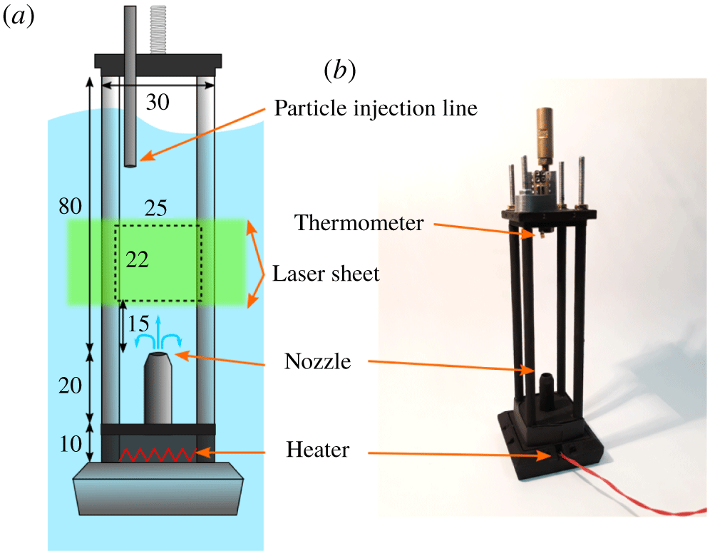
Schematic view (a) and picture (b) of the experimental cell devised for thermal generation of vortex rings. A flat resistive heater is placed at the cell bottom, below a brass circular tube, 5 mm in diameter and 20 mm high. Macroscopic vortex rings, formed above the tube, are captured in a rectangular field of view (FOV), illuminated by a planar laser sheet. The cell is attached to a mobile shaft, that is, the cell position relative to the FOV can be changed (the scheme illustrates their maximal mutual distance). A low-temperature resistive thermometer is located at the top of the cell, to measure the temperature of the He II bath. A thin capillary enters the cell to seed the fluid with solid deuterium particles. Dimensions are in millimetres.

A custom-made experimental cell was employed, see figure 1. Heat is supplied by a flat resistive heater mounted at the cell bottom. Once the heater is switched on, the normal component of the fluid flows away from it and enters a vertical circular tube, 20 mm high and of 5 mm inner diameter, open to the quiescent helium bath. For certain values of  $u_{n}$ (detailed below) and
 $t_{q}=$ 500 or 1000 ms, vortex rings having a size comparable to the tube diameter are observed a few millimetres above the tube, after the heater is switched off.
The camera field of view is 25 mm wide and 22 mm high. It is located in the middle of the channel, above the tube exit, which we call the nozzle in the following for the sake of brevity. The relative distance between the nozzle and the FOV can be adjusted because the cell is mounted on a mobile shaft and the maximum vertical distance from the nozzle accessed in the present series of experiments is equal to approximately 6 times the tube diameter  $D$. Note that, in previous experiments on macroscopic vortex rings in He II, similar distances from the nozzle were accessed.
Individual experimental realizations were carried out in a repetitive manner, i.e. several movies were consecutively collected at fixed distance from the nozzle, temperature, applied heat flux and pulse duration, provided that the waiting time between the realizations was long enough for the background flow to decay. Several data sets were obtained at temperatures between  $1.28$ and
 $1.95$ K, and for heat fluxes ranging from
 $35$ to
 $450~\text{mW}~\text{cm}^{-2}$. Note that, in the temperature range considered, the ratio
 $\unicode[STIX]{x1D70C}_{n}/\unicode[STIX]{x1D70C}$ varies from approximately 5 % to 50 % and that the presence of either of the components cannot be neglected.
The particle tracking velocimetry technique was employed to analyse the collected data sets, as in previous studies; see, for example, Švančara et al. (Reference Švančara, Hrubcová, Rotter and La Mantia2018b). The particle positions in the visualized plane are firstly detected from the video frames and linked into trajectories by using an open-source software (Sbalzarini & Koumoutsakos Reference Sbalzarini and Koumoutsakos2005). Missing positions are linearly interpolated in such a way that the sampling rate of particle trajectories matches the camera frame rate, equal to 1 or 2 kHz.
The raw trajectories are then processed in order to estimate the particle velocities. This task is carried out by convolving the raw tracks with suitable smoothing and differentiation kernels that yield the sought velocities and are robust against experimental noise, originating, for example, from the imprecise location of the particles; see Švančara, Hrubcová & La Mantia (Reference Švančara, Hrubcová, La Mantia, Šimurda and Bodnár2018a) for further details on this method.
2.1 Lagrangian pseudovorticity
The collected movies clearly depict the cross-section of vortex rings, as a pair of counter-rotating vortices, moving upward, away from the nozzle. They are made visible due to their influence on the particle motion. Indeed, the particle trajectories are often bent into loops or are dragged into the wake that is seen behind most rings.
Note in passing that our particles rarely access the ring core region because their density is approximately 40 % larger than the fluid density. Additionally, the effect of the particle inertia on the flow features is, in the present case, unknown because we only performed experiments by using deuterium particles; see, for example, Švančara et al. (Reference Švančara, Hrubcová, Rotter and La Mantia2018b) for a discussion on the role of particle density in other flows of He II.
The specific nature of the observed particle tracks motivated us to revisit the concept of Lagrangian pseudovorticity, introduced in our previous studies on the macroscopic eddies shed by objects oscillating in the liquid (Duda et al. Reference Duda, Švančara, La Mantia, Rotter and Skrbek2015, Reference Duda, La Mantia and Skrbek2017). This scalar quantity acts as a space- and time-resolved measure of the vortex strength, and its introduction was mainly justified by the fact that, by using our Lagrangian data, it is in general not possible to obtain the flow vorticity, which is an Eulerian quantity often employed to quantify the strength of vortical structures (Duda Reference Duda2017).
Here, we indicate the pseudovorticity with the symbol  $\unicode[STIX]{x1D703}$ and define it as
 $$\begin{eqnarray}\unicode[STIX]{x1D703}(\boldsymbol{r},t)=\left\langle \frac{[(\boldsymbol{r}_{i}-\boldsymbol{r})\times \boldsymbol{u}_{i}]_{z}}{|\boldsymbol{r}_{i}-\boldsymbol{r}|^{2}}\right\rangle _{{\mathcal{M}}},\end{eqnarray}$$
consistently with Duda et al. (Reference Duda, Švančara, La Mantia, Rotter and Skrbek2015, Reference Duda, La Mantia and Skrbek2017). The angle brackets denote the ensemble average within the set  ${\mathcal{M}}$ of Lagrangian particles (their two-dimensional positions and velocities are indicated as
 $\boldsymbol{r}_{i}$ and
 $\boldsymbol{u}_{i}$, respectively). The set
 ${\mathcal{M}}$ includes the particles that are found within an annular region, of 1 mm inner and 5 mm outer radii, centred, on a chosen grid, at the inspection point
 $\boldsymbol{r}$ and captured within a 10 ms time window, centred at time
 $t$. The subscript
 $z$ indicates that the observed particle trajectories occur in a plane, that is, we consider the only non-zero component of the vector product (the
 $z$ axis is perpendicular to the field of view).
The size of the annular region was chosen according to the apparent size of the observed vortex rings and, simultaneously, to exclude diverging contributions from particles too close to the inspection point  $\boldsymbol{r}$. Additionally, the data obtained from multiple realizations were merged together, in order to increase the signal-to-noise ratio.
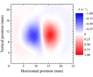
The ring visualization was performed by computing the  $\unicode[STIX]{x1D703}$ values on a square mesh of
 $115\times 101$ inspection points, covering the entire FOV. Such maps of the
 $\unicode[STIX]{x1D703}$ parameter, which we call
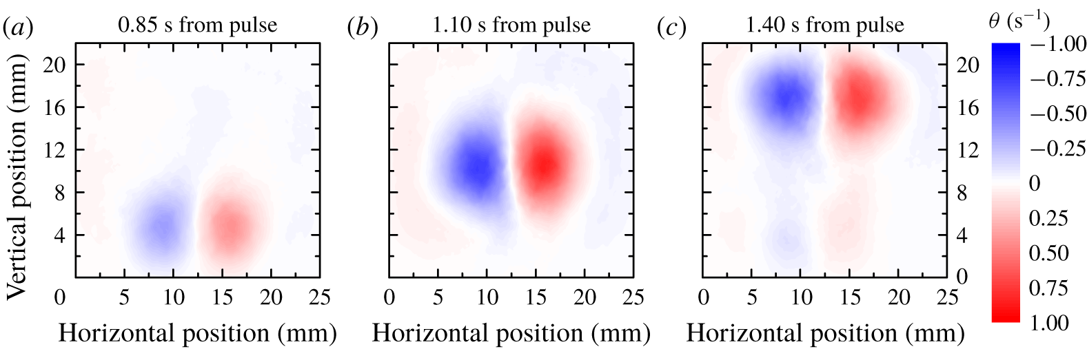
 $\unicode[STIX]{x1D703}$-maps, clearly display vortex pairs, see figure 2, and allow further quantitative processing.
We typically observe that the ring is formed near the bottom of the FOV, see figure 2(a). Then, the ring gradually propagates upward as a vortex pair, see figure 2(b), until it reaches the top of the FOV. At this stage, the regions of non-zero  $\unicode[STIX]{x1D703}$ begin to deform and eventually decay down to the noise level. Note also that the wake, formed behind the ring, is visible on figure 2(c).
Example of vortex ring visualization. The  $\unicode[STIX]{x1D703}$-maps are obtained at different times after the heat pulse, noted above the panels. In this case, the temperature was
 $1.50$ K and a heat pulse of
 $278~\text{mW}~\text{cm}^{-2}$ was applied for 500 ms, see data set 150c in table 1, shown below in § 2.3. Positive (negative) values of
 $\unicode[STIX]{x1D703}$ indicate clockwise (counter-clockwise) rotation. Note the neatly visible ring wake in the right panel. The vertical coordinate indicates the distance from the nozzle and the reference system origin is at the bottom left corner of the field of view; 10 realizations (movies) were averaged before calculating the
 $\unicode[STIX]{x1D703}$-maps.

The parameter  $\unicode[STIX]{x1D703}$ was called pseudovorticity because, following Duda (Reference Duda2017), we expected that, in the ideal condition of infinitely dense sampling, which is not met in experiments,
 $\unicode[STIX]{x1D703}$ converges to the flow vorticity normal to the observation plane. However, one referee of the present work found a mistake in the just mentioned proof, connecting
 $\unicode[STIX]{x1D703}$ to the vorticity, namely equation (2.20) in Duda (Reference Duda2017) does not hold. We therefore provide here a proof that quantitatively relates the Lagrangian pseudovorticity to the Eulerian vorticity, again under ideal conditions, which are not met in experiments.
To this end, we define the pseudovorticity as
 $$\begin{eqnarray}\unicode[STIX]{x1D73D}(\boldsymbol{r})=\frac{1}{N}\int _{D(\boldsymbol{r})}n(\boldsymbol{r}^{\prime })\frac{\boldsymbol{r}^{\prime }-\boldsymbol{r}}{|\boldsymbol{r}^{\prime }-\boldsymbol{r}|^{2}}\times \boldsymbol{u}(\boldsymbol{r}^{\prime })\,\text{d}^{2}\boldsymbol{r}^{\prime },\end{eqnarray}$$
where  $D(\boldsymbol{r})$ is a circle, centred at
 $\boldsymbol{r}$, with radius
 $R$, and
 $$\begin{eqnarray}N=\int _{D(\boldsymbol{r})}n(\boldsymbol{r}^{\prime })\,\text{d}^{2}\boldsymbol{r}^{\prime }=n\unicode[STIX]{x03C0}R^{2}\end{eqnarray}$$
indicates the number of particles in the circle. The distribution  $n(\boldsymbol{r})$ of particles in a plane, which is equal to the number of particles in a local domain divided by the area of that domain, is here assumed to be constant, that is, the particles are homogeneously distributed in the circle. Additionally, we assume that the fluid has a smooth velocity field
 $\boldsymbol{u}(\boldsymbol{r})$ and that the particle velocity at point
 $\boldsymbol{r}$ is equal to
 $\boldsymbol{u}(\boldsymbol{r})$.
We can now use the Taylor expansion of the particle velocity, with respect to the difference  $\unicode[STIX]{x0394}\boldsymbol{r}=\boldsymbol{r}^{\prime }-\boldsymbol{r}$, and write
 $$\begin{eqnarray}u_{i}(\boldsymbol{r}^{\prime })=u_{i}(\boldsymbol{r})+\unicode[STIX]{x0394}r_{j}\unicode[STIX]{x2202}_{j}u_{i}(\boldsymbol{r})+{\textstyle \frac{1}{2}}\unicode[STIX]{x0394}r_{j}\unicode[STIX]{x0394}r_{k}\unicode[STIX]{x2202}_{j}\unicode[STIX]{x2202}_{k}u_{i}(\boldsymbol{r}),\end{eqnarray}$$
neglecting higher-order terms, which is allowed by the smoothness of  $\boldsymbol{u}(\boldsymbol{r})$; note that, here, the Einstein summation is employed and that
 $\unicode[STIX]{x2202}_{j}u_{i}$ indicates the partial derivative of the
 $i$ component of the vector
 $\boldsymbol{u}$ with respect to the
 $j$ coordinate. By using (2.2) and (2.4) we obtain
 $$\begin{eqnarray}\unicode[STIX]{x1D703}_{i}(\boldsymbol{r})=I_{1}+I_{2}+I_{3},\end{eqnarray}$$
where
 $$\begin{eqnarray}\displaystyle & \displaystyle I_{1}=\frac{n}{N}\unicode[STIX]{x1D716}_{ijk}\int _{D(\boldsymbol{r})}\frac{\unicode[STIX]{x0394}r_{j}}{|\unicode[STIX]{x0394}\boldsymbol{r}|^{2}}\,\text{d}^{2}\boldsymbol{r}^{\prime }u_{k}(\boldsymbol{r}), & \displaystyle\end{eqnarray}$$
 $$\begin{eqnarray}\displaystyle & \displaystyle I_{2}=\frac{n}{N}\unicode[STIX]{x1D716}_{ijk}\int _{D(\boldsymbol{r})}\frac{\unicode[STIX]{x0394}r_{j}}{|\unicode[STIX]{x0394}\boldsymbol{r}|^{2}}\unicode[STIX]{x0394}r_{l}\,\text{d}^{2}\boldsymbol{r}^{\prime }\unicode[STIX]{x2202}_{l}u_{k}(\boldsymbol{r}), & \displaystyle\end{eqnarray}$$
and
 $$\begin{eqnarray}I_{3}=\frac{n}{N}\unicode[STIX]{x1D716}_{ijk}\int _{D(\boldsymbol{r})}\frac{\unicode[STIX]{x0394}r_{j}}{|\unicode[STIX]{x0394}\boldsymbol{r}|^{2}}\frac{1}{2}\unicode[STIX]{x0394}r_{l}\unicode[STIX]{x0394}r_{m}\,\text{d}^{2}\boldsymbol{r}^{\prime }\unicode[STIX]{x2202}_{l}\unicode[STIX]{x2202}_{m}u_{k}(\boldsymbol{r});\end{eqnarray}$$
note that  $\unicode[STIX]{x1D716}_{ijk}$ indicates the Levi-Civita symbol in three dimensions.
If, in the above integrals, we use the substitutions  $\boldsymbol{r}^{\prime }\rightarrow \unicode[STIX]{x0394}\boldsymbol{r}\rightarrow -\unicode[STIX]{x0394}\boldsymbol{r}$, we find that
 $I_{1}=I_{3}=0$, while
 $I_{2}$ only does not vanish for
 $j=l$ because
 $$\begin{eqnarray}\int _{D(\boldsymbol{r})}\frac{(\unicode[STIX]{x0394}r_{j})^{2}}{|\unicode[STIX]{x0394}\boldsymbol{r}|^{2}}\,\text{d}^{2}\boldsymbol{r}^{\prime }=\int _{D(0)}\frac{(\unicode[STIX]{x0394}r_{j})^{2}}{|\unicode[STIX]{x0394}\boldsymbol{r}|^{2}}\,\text{d}^{2}\unicode[STIX]{x0394}\boldsymbol{r}=\int _{0}^{2\unicode[STIX]{x03C0}}\int _{0}^{R}\frac{r^{2}\cos ^{2}\unicode[STIX]{x1D719}}{r^{2}}r\,\text{d}r\,\text{d}\unicode[STIX]{x1D719}=\frac{\unicode[STIX]{x03C0}R^{2}}{2},\end{eqnarray}$$
where suitable polar coordinates are used for the calculation of the integral. It then follows that (2.5) becomes
 $$\begin{eqnarray}\unicode[STIX]{x1D703}_{i}(\boldsymbol{r})={\textstyle \frac{1}{2}}\unicode[STIX]{x1D716}_{ijk}\unicode[STIX]{x2202}_{j}u_{k}(\boldsymbol{r}),\end{eqnarray}$$
which means that the pseudovorticity is half of the vorticity, in the close vicinity of  $\boldsymbol{r}$, for a homogeneous distribution of fluid particles having a smooth velocity field.
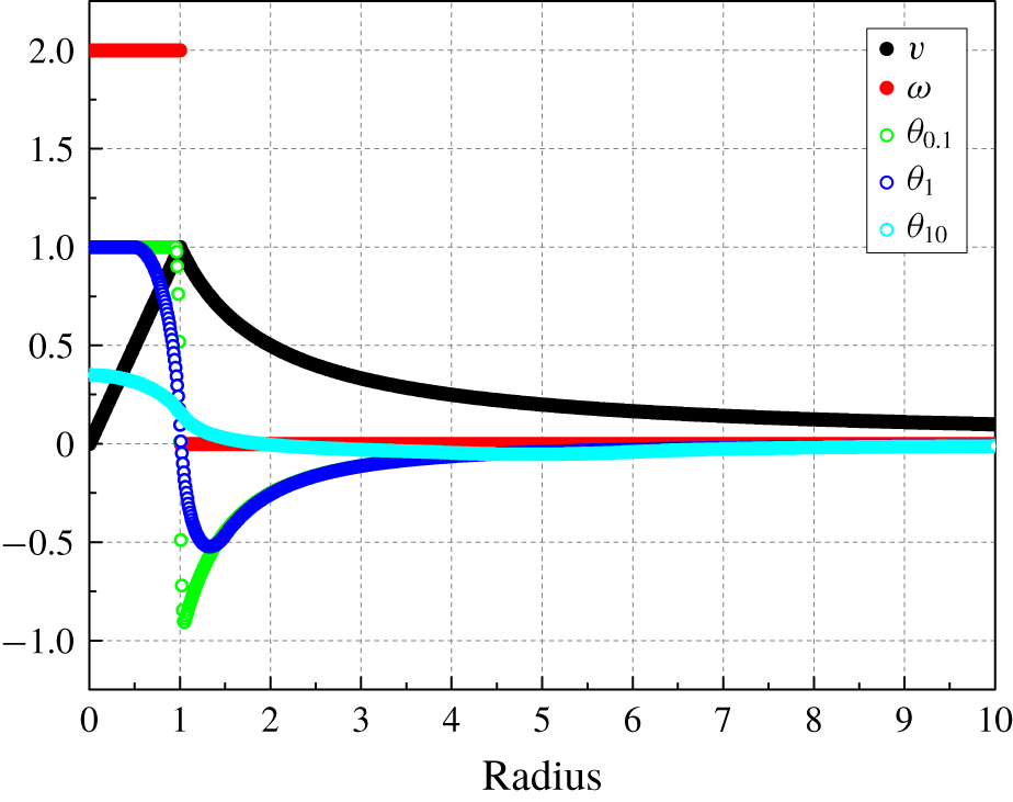
Pseudovorticity for a Rankine vortex as a function of the distance from the vortex axis (radius). Black circles: vortex velocity  $v$; red circles: vorticity
 $\unicode[STIX]{x1D714}$; open circles: pseudovorticity
 $\unicode[STIX]{x1D703}$, the corresponding subscripts in the legend indicate the ratio between the radius of the area used for the calculation of
 $\unicode[STIX]{x1D703}$, equation (2.1), and the vortex radius where the abrupt vorticity change occurs, set to one; see the text for details.

It can be shown that the same result holds for an isotropic particle distribution, but, if  $n(\boldsymbol{r})$ is neither homogeneous nor isotropic, the relation between pseudovorticity and vorticity will be affected by the actual particle distribution in the chosen area. Additionally, our particles are not fluid particles and the area considered in (2.1) cannot be said to be in the close proximity of the inspection point (a large enough number of particle positions and velocities is needed for the experimental estimation of
 $\unicode[STIX]{x1D703}$).
For the sake of argument, we also calculated the pseudovorticity for a Rankine vortex by using (2.1). We specifically changed the size of the area employed to estimate  $\unicode[STIX]{x1D703}$, but we kept in this area the same number of homogenously distributed particles (we did not calculate
 $\unicode[STIX]{x1D703}$ at the area centre). Indeed, it is apparent from figure 3 that, as the size of this region becomes smaller, the pseudovorticity tends to half of the vorticity, if one neglects the region where the fluid velocity is not smooth enough.
The previous remarks not only justify the name given to the parameter  $\unicode[STIX]{x1D703}$, but also show that the pseudovorticity can be conveniently used to estimate the strength of vortical structures, if other means are not available, as in our case. On the other hand, it should also be evident to the reader that, at present, a general, quantitative relation between
 $\unicode[STIX]{x1D703}$ and the actual flow vorticity is yet to be established, and that its determination is outside the scope of the present experimental work on macroscopic vortex rings propagating in He II.
2.2 Identification and tracking of vortex rings
The observed vortex pairs can be separated from the background flow by setting a (positive) threshold  $\unicode[STIX]{x1D703}_{0}$. The positive (clockwise) vortex then consists only of mesh points (pixels) with
 $\unicode[STIX]{x1D703}>\unicode[STIX]{x1D703}_{0}$, the negative (counter-clockwise) one is instead characterized by
 $\unicode[STIX]{x1D703}<-\unicode[STIX]{x1D703}_{0}$. Threshold values ranging between
 $0.15$ and
 $0.25$ s
 $^{-1}$ were chosen in accordance with the corresponding level of background noise.
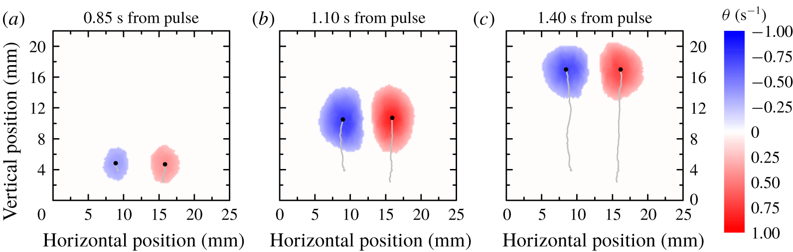
An example of the method is shown in figure 4, with  $\unicode[STIX]{x1D703}_{0}=0.25~\text{s}^{-1}$. At the beginning, see figure 4(a), only a few pixels pass the threshold, but, when the ring is fully developed, large circular regions appear, see figure 4(b,c). One can then define the positions
 $\boldsymbol{P}_{p}$ and
 $\boldsymbol{P}_{n}$, for the positive and negative vortices, respectively, as the
 $\unicode[STIX]{x1D703}$-weighted centres of these regions, which are displayed in figure 4 as black points (the grey lines indicate the corresponding tracks).
Following Gan & Nickels (Reference Gan and Nickels2010), we define the diameter of the vortex ring as  $2R=|\boldsymbol{P}_{p}-\boldsymbol{P}_{n}|$. Additionally, the position
 $\boldsymbol{P}$ of the vortex ring itself is defined as the joint,
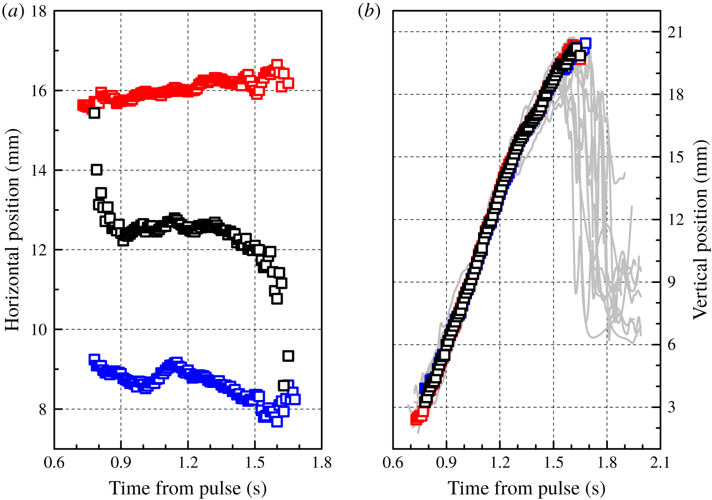
 $\unicode[STIX]{x1D703}$-weighted centre of the two vortices. Figure 5 shows typical results of this tracking procedure. The two panels display the Cartesian components of
 $\boldsymbol{P}$ (black open squares),
 $\boldsymbol{P}_{p}$ and
 $\boldsymbol{P}_{n}$ (red and blue open squares, respectively). It is evident from the figure that the rings move in the vertical direction. Some outlying data points can be spotted at the extrema of the time series. At its beginning, the behaviour is likely due to the weak signal because the size of the regions that pass the threshold value is very small. On the other hand, at the end of the tracking interval, the rings are deformed as they approach the top of the camera FOV.
Example of vortex ring identification. The threshold  $\unicode[STIX]{x1D703}_{0}=0.25~\text{s}^{-1}$ is employed to detect the rings from the
 $\unicode[STIX]{x1D703}$-maps plotted in figure 2. The black points denote the region centres and the grey lines indicate the corresponding trajectories; see the text for details.

Result of the tracking scheme for the ring plotted in figure 4. Red and blue open squares: positions  $\boldsymbol{P}_{p}$ and
 $\boldsymbol{P}_{n}$, respectively; black open squares: position
 $\boldsymbol{P}$ of the vortex ring. (a) Horizontal ring position relative to the camera field of view as a function of the time elapsed from the end of the heat pulse. (b) Vertical position relative to the nozzle; the solid grey lines indicate the vertical positions of the 10 individual realizations collected at these experimental conditions; see the text for details.

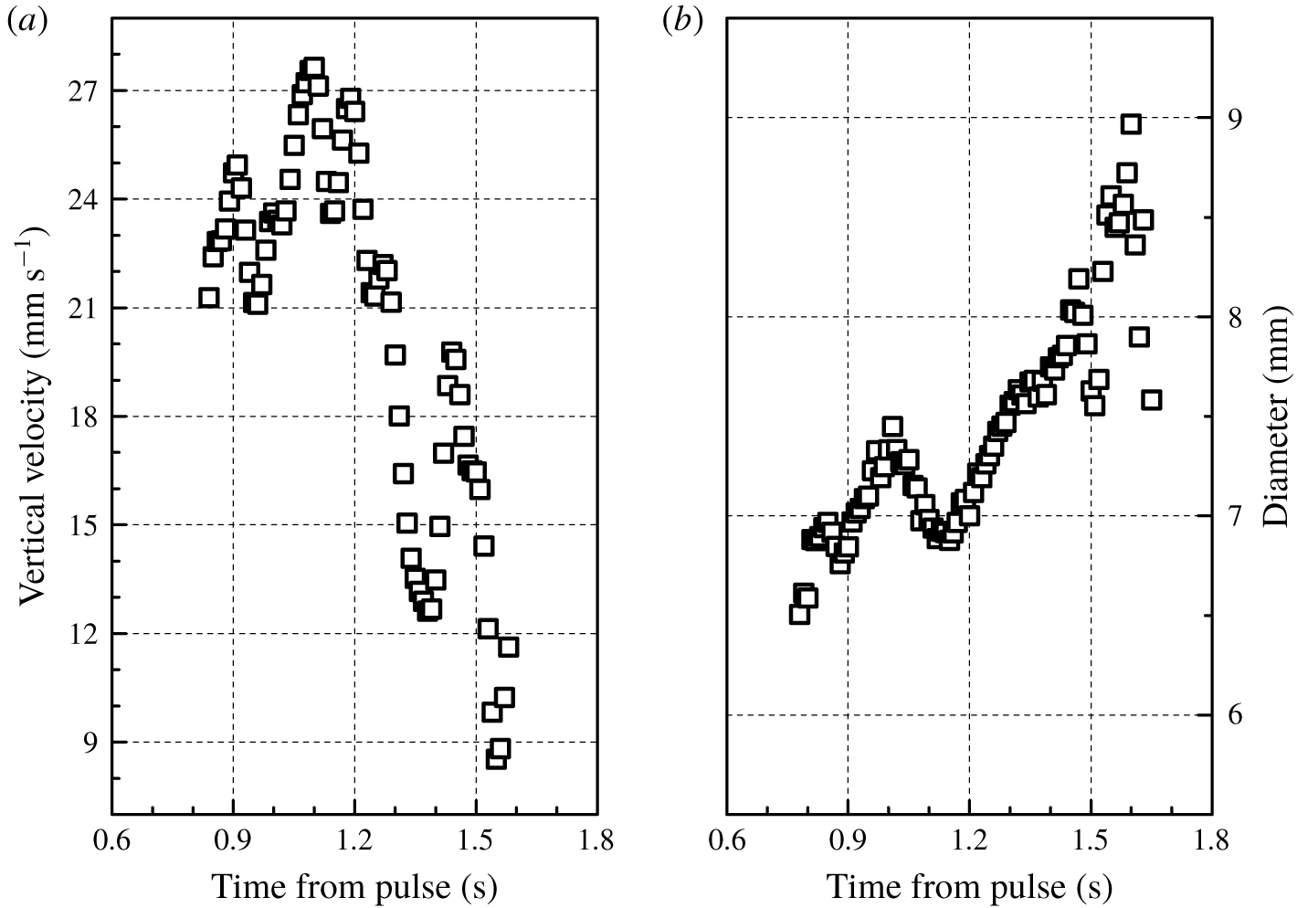
(a) Vertical velocity of the ring tracked in figure 5 as a function of the time elapsed from the end of the heat pulse. (b) Diameter  $2R$ of the same ring.

The ring velocity can be estimated as that of individual particles, by convolving  $\boldsymbol{P}$ with a suitable Gaussian kernel. Figure 6(a) displays the ring vertical velocity, i.e. the time derivative of the data shown in figure 5(b), as a function of time. The obtained velocity indicates that the ring is likely slowing down, at large enough times. Similarly, the ring diameter
 $2R$ appears to increase with time, see figure 6(b).
Note that oscillations are apparent in the velocity and diameter time series. They may originate from azimuthal oscillations of the vortex ring, which were observed, for example, by Maxworthy (Reference Maxworthy1977) and Sullivan et al. (Reference Sullivan, Niemela, Hershberger, Bolster and Donnelly2008). Additionally, it cannot be excluded that the ring is actually not propagating along planes exactly perpendicular to the camera FOV and this could also contribute to explaining the  $\boldsymbol{P}$ slope change in figure 5(b).
To summarize, the just outlined data processing scheme consists of (i) particle tracking, (ii) particle velocity estimation, (iii) calculation of  $\unicode[STIX]{x1D703}$-maps, (iv) vortex ring identification and tracking and (v) estimation of the ring size, position and velocity. The resulting data are quantitative and may serve as a relatively simple tool for the Lagrangian study of macroscopic vortex rings.
2.3 Ring generation reproducibility
Azimuthal instabilities and asymmetric ring interactions with the surrounding fluid may lead to the finite dispersion of the ring trajectories. This phenomenon was experimentally observed, for example, by Gan & Nickels (Reference Gan and Nickels2010), at relatively large distances from the nozzle. Although the present study is focused on shorter distances, the reproducibility of the ring generation process was explicitly tested.
For this purpose, 10 realizations of vortex rings, obtained at  $1.50$ K, with a heat flux of
 $278$ mW cm
 $^{-2}$ applied for 500 ms, were processed separately in order to obtain their respective trajectories, that is, we analysed separately the 10 movies collected at these experimental conditions. Figure 5(b) displays the vertical position as a function of time for the 10 movies (grey lines) together with the same quantity calculated from the entire data set, which includes all the 10 realizations (open black squares). From the figure, it appears that ring generation is a reproducible process, especially at sufficiently small times, that is, the outcome supports the use of ensemble averaging in the present conditions.
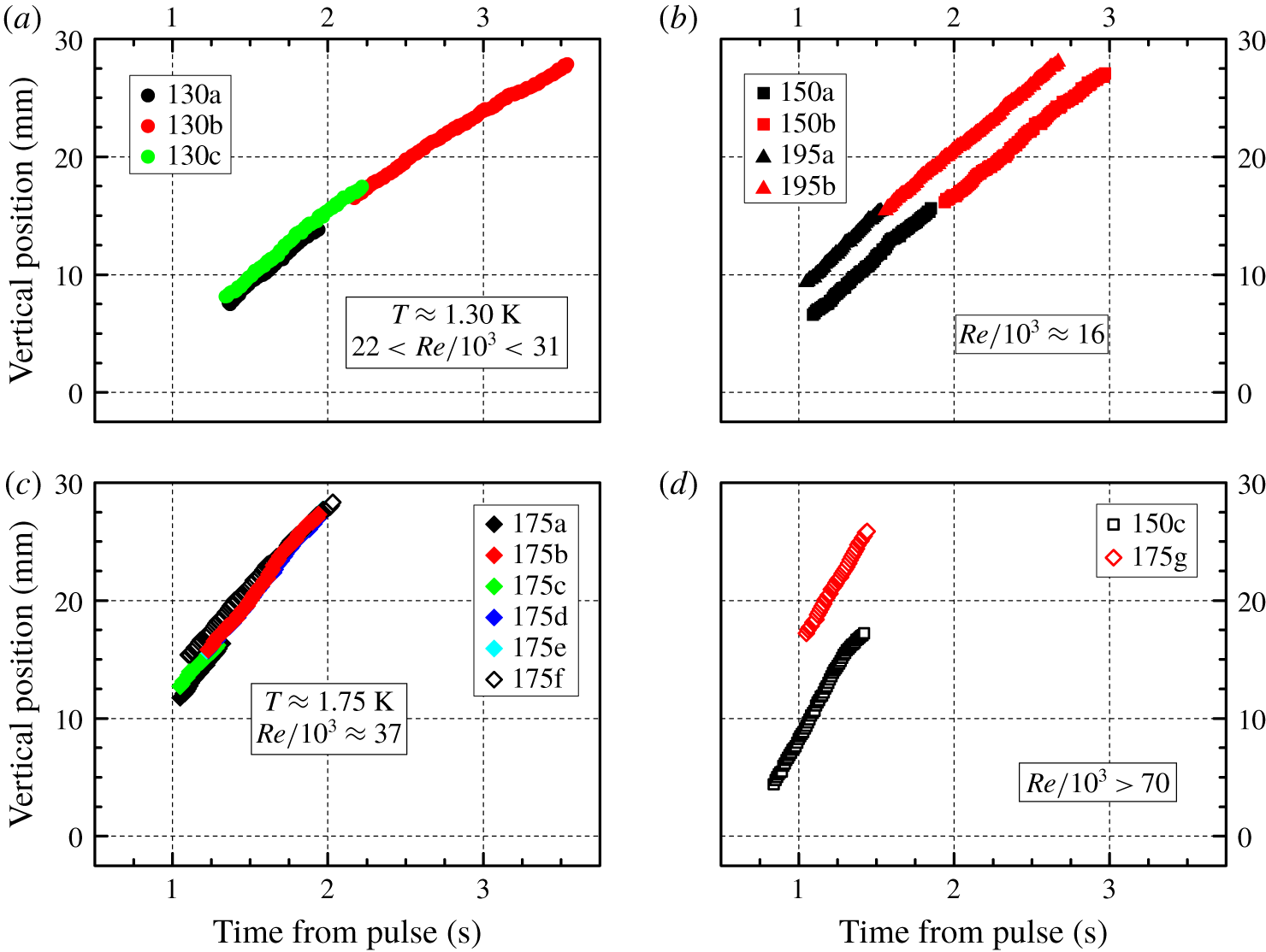
Ring vertical position, relative to the nozzle, as a function of the time elapsed from the end of the heat pulse. The legends indicate the plotted data sets, see table 1 for the corresponding experimental conditions; for the sake of clarity, the results are displayed in different panels, depending on Reynolds number and temperature, which are indicated as appropriate in each panel. Note that positions obtained in similar conditions overlap, see, for example, the data sets 175b, 175d and 175e in the bottom left panel.

However, it is also apparent from figure 5(b) that, for times larger than approximately  $1.4$ s, individual ring trajectories are much more scattered, and, additionally, a sudden position decrease is observed in most cases. This is likely due to the ring being close to the FOV top and to the signal coming from its wake (note that ensemble averaging is carried out only if the ring vertical position is detected in all the realizations). Additionally, for the entire data set, more points contribute to the calculation of
 $\unicode[STIX]{x1D703}$-maps and the background signal, which includes the wake, is reduced. Nevertheless, the latter signal could also contribute to explaining the
 $\boldsymbol{P}$ slope change in figure 5(b).
The reproducibility of the ring generation process was also tested from another perspective. As mentioned above, some data sets were obtained by visualizing the region close to the nozzle and others from the visualization of areas further away from it. We specifically find that data obtained in similar experimental conditions overlap, if we match the time origin with the end of the heat pulse and if the position origin coincides with the nozzle, see, for example, figure 7. The outcome strongly supports the view that the devised set-up can consistently generate vortex rings and that their dynamics depends on the chosen experimental conditions in a reproducible way.
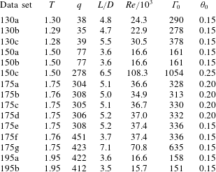
Experimental conditions: temperature  $T$, in K; applied heat flux
 $q$, in
 $\text{mW}~\text{cm}^{-2}$; ratio between the stroke length
 $L=u_{n}t_{q}$, where
 $u_{n}$ indicates the normal fluid velocity, equation (1.2), and the nozzle diameter
 $D=5~\text{mm}$; the heat pulse duration
 $t_{q}$ is equal to 500 ms for data sets 150c and 175f, while
 $t_{q}=1000$ ms for the other cases; Reynolds number
 $Re$ and nominal circulation
 $\unicode[STIX]{x1D6E4}_{0}$, in
 $\text{mm}^{2}~\text{s}^{-1}$, equation (1.3); chosen pseudovorticity threshold
 $\unicode[STIX]{x1D703}_{0}$, in s
 $^{-1}$, for ring identification.

It is now useful to remark that the values of applied heat flux  $q$ listed in table 1 are averaged over the heat pulse duration
 $t_{q}$ and that the heat flux sampling frequency for the current series of experiments was 4 Hz, that is, we applied a chosen power to the heater and, during the heat pulse, we measured the actual power supplied to the heater with a frequency of 4 Hz, taking into account the relatively small power dissipated by the wires. It then follows that, at present, we cannot precisely say how the normal fluid velocity
 $u_{n}$, which is proportional to the heat flux, varied with time, during the heat pulse. Additionally, in order to make relevant comparisons, detailed below, we established above the analogy between
 $u_{n}$ and the piston velocity
 $U_{p}$, see (1.3). We have therefore to remind the reader that, as reported, for example, by Glezer (Reference Glezer1988), the time dependence of the piston velocity may have a significant effect on the observed features of the generated vortex rings. Consequently, the fact that we do not have detailed information on the time behaviour of the applied heat flux is a limitation of the current series of experiments, but, on the other hand, once stated, it allows us to proceed with the analysis by considering the Reynolds numbers listed in table 1 as useful first-order estimates.
3 Results and discussion
It is evident from table 1 that, for the present series of experiments, the Reynolds number  $Re$, calculated by using (1.3), ranges between approximately
 $15\times 10^{3}$ and
 $11\times 10^{4}$. It follows that our rings can be said to be in the turbulent regime because Glezer (Reference Glezer1988) reported that turbulent rings are observed for
 $Re\gtrsim 10^{4}$. Additionally, the ratio between our stroke length
 $L$ and the nozzle diameter
 $D=5~\text{mm}$ is approximately 5 – see table 1 – and it has been reported by Gharib, Rambod & Shariff (Reference Gharib, Rambod and Shariff1998) that wake formation is usually observed for
 $L/D\gtrsim 4$, which is consistent with our findings, see, for example, figure 2(c). The reader should, however, keep in mind the assumptions made for the derivation of (1.3), that is, as mentioned above, the Reynolds numbers listed in table 1 should solely be regarded as first-order estimates, mainly because superfluid 4He cannot, in general, be described as if it were a classical viscous fluid like water.
3.1 Ring position and diameter
We plot in figure 7 the ring vertical position  $y$ as a function of the time elapsed from the end of the heat pulse for all the data sets considered here; see table 1 for the relevant experimental conditions. We display solely positions obtained when the ring is fully visible within the camera field of view, that is, we neglect early and late times, following the procedure discussed above.
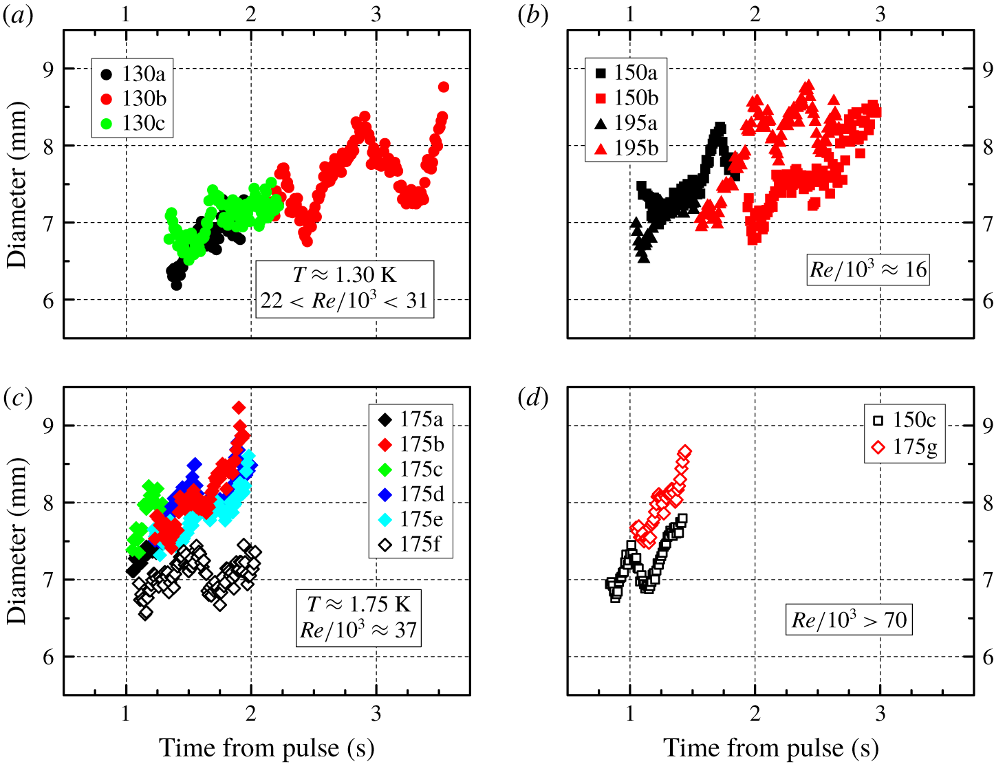
Ring diameter  $2R$ as a function of the time elapsed from the end of the heat pulse. Symbols and panel description as in figure 7.

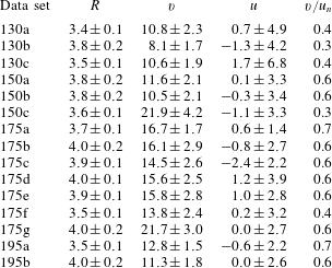
Experimental results: ring radius  $R$, in mm; ring vertical velocity
 $v$, in
 $\text{mm}~\text{s}^{-1}$; ring horizontal velocity
 $u$, in
 $\text{mm}~\text{s}^{-1}$; ratio between the mean value of the ring vertical velocity
 $v$ and the normal fluid velocity
 $u_{n}$, equation (1.2). Note that for each case at least 1 million particle positions were used for the analysis.

It can be noted that the rings move upward and that, in similar experimental conditions, the data sets have similar slopes. Additionally, the plots obtained for  $Re>70\times 10^{3}$ – see figure 7(d) – are significantly steeper than the others, although a straightforward relation between the slope and the Reynolds number is not apparent from the current data sets.
The ring diameter  $2R$ is shown in figure 8 as a function of the time elapsed from the end of the heat pulse. As explained above, it was computed by applying to the obtained
 $\unicode[STIX]{x1D703}$-maps the relevant pseudovorticity threshold
 $\unicode[STIX]{x1D703}_{0}$ listed in table 1. We also report in table 2 corresponding mean values and standard deviations for ring radii.
It is evident from figure 8 that the ring diameter – which can be regarded as a first-order estimate of the ring size – shows, in most cases, the tendency to increase as the distance from the nozzle becomes larger, that is, with time. This outcome is consistent not only with the classical behaviour – see, for example, Maxworthy (Reference Maxworthy1974) – but also with results obtained in He II (Murakami et al. Reference Murakami, Hanada and Yamazaki1987; Stamm et al. Reference Stamm, Bielert, Fiszdon and Piechna1994a). Note in passing that in previous vortex ring experiments in superfluid 4He the nominal circulation  $\unicode[STIX]{x1D6E4}_{0}\approx 1000~\text{mm}^{2}~\text{s}^{-1}$, that is, the present Reynolds numbers are, in most cases, smaller than those obtained in the past.
Additionally, the ring size oscillates and, as mentioned above, this could be related to the presence of azimuthal waves and/or to the deviation of the ring motion from the vertical axis. Consider also that, in the range of investigated parameters, the ring diameter does not appear to depend significantly on the Reynolds number.
3.2 Ring velocity
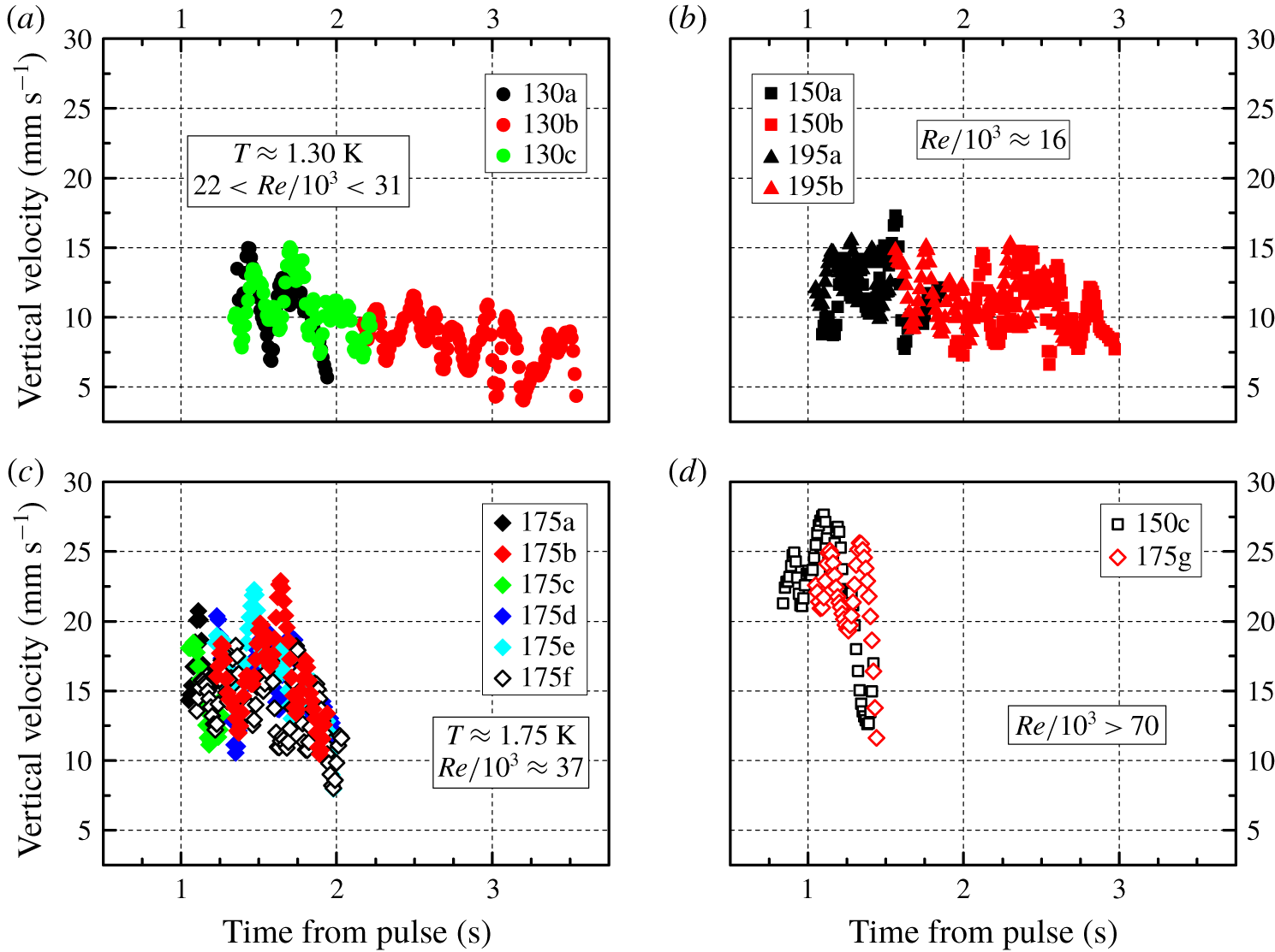
We plot in figure 9 the ring vertical velocity  $v$ as a function of the time elapsed from the end of the heat pulse, and in table 2 we list corresponding mean values and standard deviations for the ring velocities.
Ring vertical velocity  $v$ as a function of the time elapsed from the end of the heat pulse. Symbols and panel description as in figure 7.

First of all, we see in table 2 that, in the range of investigated parameters, the ring mean velocity in the vertical direction is approximately two times smaller than the normal fluid velocity  $u_{n}$, which we indicated above to be analogous to the piston velocity
 $U_{p}$, see (1.3).
This result broadly agrees not only with classical observations – see, for example, Sullivan et al. (Reference Sullivan, Niemela, Hershberger, Bolster and Donnelly2008) and references therein – but also with superfluid experiments (Borner et al. Reference Borner, Schmeling and Schmidt1983; Stamm et al. Reference Stamm, Bielert, Fiszdon and Piechna1994a), although, for the present data, the ring velocity seems to be, in most cases, closer to  $U_{p}$ than in previous investigations. This indicates that the normal fluid velocity
 $u_{n}$, computed here by using the heater area, see (1.2), most likely underestimates the actual fluid velocity inside our tube, which we cannot at present measure, especially if one takes into account that, as mentioned above, the heat flux time dependence is not precisely known.
Additionally, this remark might explain why the slopes of the data set 175f in figures 7 and 8 are different from those of other data sets obtained in similar conditions. Indeed, if we consider that, for the latter data sets, the heat pulse lasted two times longer than for case 175f, it follows that in the former cases the actual fluid velocity inside our tube might have been less unsteady than for the data set 175f, due to the different pulse durations.
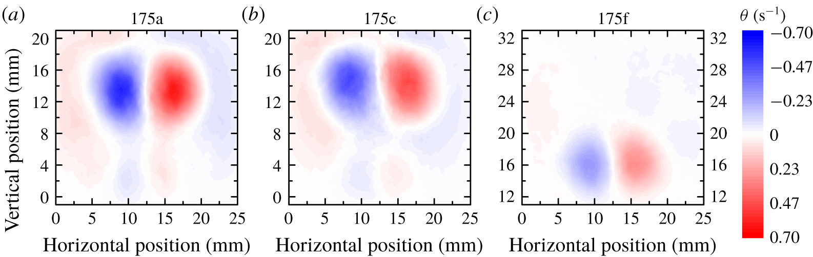
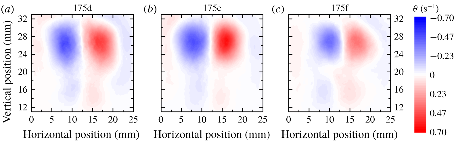
Panels (a–c) display  $\unicode[STIX]{x1D703}$-maps for different data sets, noted above the panels, obtained 1.15 s after the heat pulse; see tables 1 and 2 for details on the data set features. Note that in the right panel the vertical axis, which indicates the distance from the nozzle, has a different scale compared to the other two.


The claim is supported if one looks at relevant pseudovorticity maps, which are plotted in figures 10 and 11 for early and late times, respectively. It is evident that the ring associated with the data set 175f is characterized by smaller radius and pseudovorticity magnitudes, compared to the other rings, which have instead similar sizes and  $|\unicode[STIX]{x1D703}|$ values. It then follows that, in future experiments on thermally generated vortex rings, special care should be taken to monitor in detail the heat pulse time history.
We can also see in table 2 that, in some cases, the mean value of the ring horizontal velocity is not null and this supports the idea that the diameter oscillations shown in figure 8 are likely due to the ring trajectory dispersion and/or to the presence of azimuthal waves. Indeed, oscillations are also apparent in the vertical velocity plots of figure 9.
Nevertheless, the main conclusion that can be drawn from figures 8 and 9 is that, as time increases, the rings show a tendency to slow down and become bigger, as is expected to occur in any viscous fluid, due to energy dissipation. Consequently, if we also consider that an isolated quantized vortex loop shrinks and accelerates as it decays, due to its fixed circulation, it can be said that the macroscopic rings we are discussing here display distinctive classical-like features, which is also consistent with the results obtained in previous Lagrangian studies of other He II flows; see, for example, Švančara & La Mantia (Reference Švančara and La Mantia2017).
We can now substantiate the claim that we are currently probing flow scales larger than the mean distance  $\ell$ between quantized vortices by using the results presented above. Following Duda et al. (Reference Duda, Švančara, La Mantia, Rotter and Skrbek2015), we can say that the smallest scale
 $\ell _{exp}$ probed by our particles is equal to the mean vertical velocity of the ring multiplied by the time between subsequent particle positions. The latter is, in the present case, set to
 $0.01$ s by the smoothing scheme used to compute particle positions and velocities from the raw data (Švančara et al. Reference Švančara, Hrubcová, La Mantia, Šimurda and Bodnár2018a), while the former is listed in table 2. We obtain that, in the range of investigated parameters,
 $\ell _{exp}$ is of the order of 100
 $\unicode[STIX]{x1D707}$m, which is a value significantly larger than the typical size of our particles (Švančara & La Mantia Reference Švančara and La Mantia2017). We can compute the mean distance between quantized vortices as
 $$\begin{eqnarray}\ell =R\left(\frac{\unicode[STIX]{x1D705}}{\unicode[STIX]{x1D6E4}_{0}}\right)^{1/2},\end{eqnarray}$$
where we assume that  $\unicode[STIX]{x1D6E4}_{0}/\unicode[STIX]{x1D705}$ quantized vortex loops are present within each macroscopic vortex ring, following Wacks et al. (Reference Wacks, Baggaley and Barenghi2014), who showed that, above 1 K, in the two-fluid regime of He II, bundles of quantized vortex loops appear stable and similar to classical vortex rings; relevant values of the ring nominal circulation
 $\unicode[STIX]{x1D6E4}_{0}$ are listed in table 1 and
 $\unicode[STIX]{x1D705}=9.97\times 10^{-8}~\text{m}^{2}~\text{s}^{-1}$ is the quantum of circulation associated with each quantized vortex. By using the mean values of the ring radius listed in table 2 we obtain that
 $\ell _{exp}$ is approximately two times larger than
 $\ell$. We can then say that, to a first approximation, our claim is verified, but, at the same time, to give a more robust estimate of the mean distance between quantized vortices, one should know the actual ring vorticity distribution and, in the following section, we discuss if this is possible by using the present experimental data.
3.3 Ring circulation and area
In order to calculate the ring circulation, one could start from the knowledge of the flow vorticity, but, at present, we only have information on the Lagrangian pseudovorticity and, as mentioned above, a general, quantitative relation between these two quantities does not currently exist. On the other hand, one may estimate the ring circulation by using the experimentally obtained pseudovorticity values and then compare the outcome to the behaviour of the ring circulation reported in the literature, in view of assessing the relevance of our  $\unicode[STIX]{x1D703}$-maps for the actual flow vorticity.
We decided to follow this route, that is, we estimate the ring circulation  $C$ from the pseudovorticity values, calculated on a square mesh of
 $115\times 101$ points, covering the entire field of view. We specifically use the relation
 $$\begin{eqnarray}C=\displaystyle \frac{C_{p}-C_{n}}{2}=\frac{\displaystyle \sum (\unicode[STIX]{x1D703}_{p}a)-\displaystyle \sum (\unicode[STIX]{x1D703}_{n}a)}{2},\end{eqnarray}$$
where the summations take solely into account the mesh points passing the threshold  $\unicode[STIX]{x1D703}_{0}$; the subscript
 $p$ (
 $n$) indicates that the corresponding
 $\unicode[STIX]{x1D703}$ values are positive (negative) and
 $a\approx 0.05~\text{mm}^{2}$ denotes the area of the field of view associated with each mesh point. We found that
 $C_{p}\approx |C_{n}|$ and therefore focus here on the corresponding mean value
 $C$, as defined in (3.2).
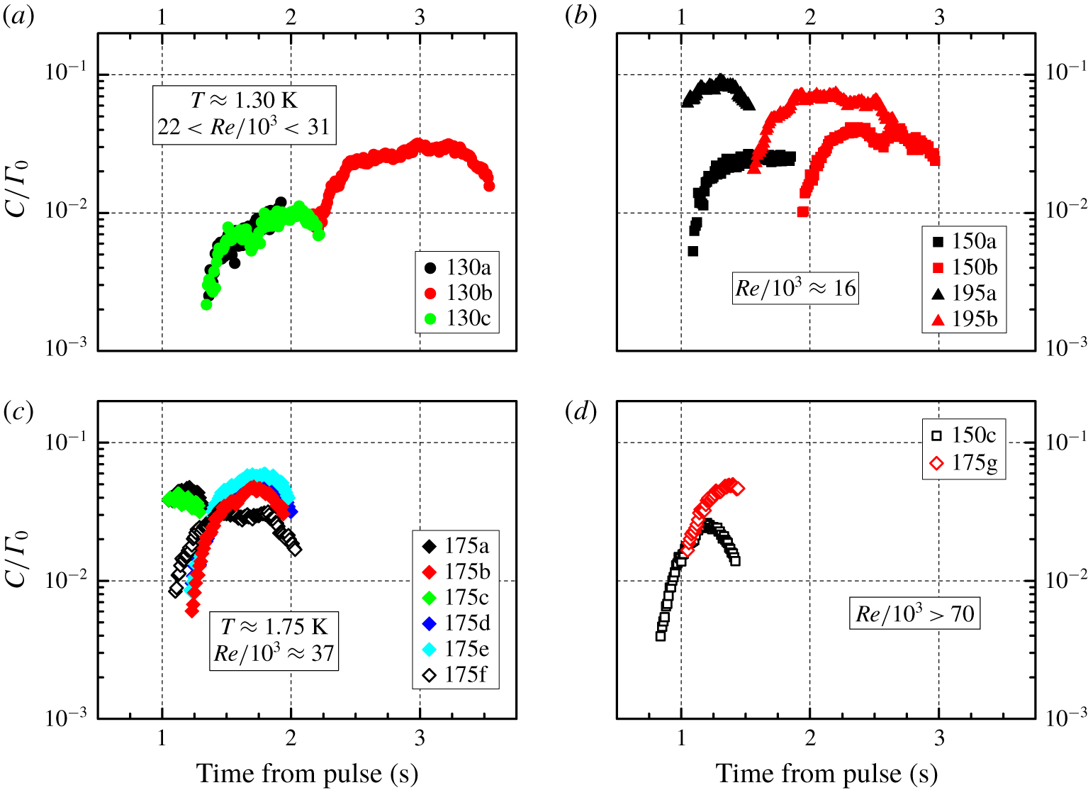
We plot in figure 12 the ratio  $C/\unicode[STIX]{x1D6E4}_{0}$ as a function of the time elapsed from the end of the heat pulse. The first feature one may notice is that, in the range of investigated parameters,
 $\unicode[STIX]{x1D6E4}_{0}$ is much larger than the calculated
 $C$ values, by up to approximately two orders of magnitude. The outcome clearly indicates that, in the present case, the pseudovorticity magnitude is much smaller than that of the expected flow vorticity, if one considers that experimental results obtained by Maxworthy (Reference Maxworthy1977), for turbulent rings, and Didden (Reference Didden1979), in the laminar case, show that measured values of the ring circulation are of the same order as
 $\unicode[STIX]{x1D6E4}_{0}$, at least close enough to the nozzle and for
 $L/D\approx 1$ (a similar outcome was reported by Borner & Schmidt (Reference Borner, Schmidt, Meier and Obermeier1985) for He II ring experiments). We therefore believe that such a large discrepancy between the expected and computed magnitudes of the ring circulation clearly indicates that the magnitude of our
 $\unicode[STIX]{x1D703}$ parameter is not equal to that of the actual flow vorticity.
Ratio between the ring circulations  $C$ and
 $\unicode[STIX]{x1D6E4}_{0}$ as a function of the time elapsed from the end of the heat pulse; see the text for details. Symbols and panel description as in figure 7.

The time dependence of  $C$ is also not consistent with previous results. Indeed, for turbulent rings, the circulation is expected to decrease with time, as discussed, for example, by Maxworthy (Reference Maxworthy1974). Similarly, it was shown by Didden (Reference Didden1979) that the circulation of laminar rings increases solely at early times, during the formation process, at distances from the nozzle of the order of the latter diameter, and then, at later times, it decreases too. If one considers that the data shown in figure 12 were obtained at distances larger than the nozzle diameter, that is, most likely after the formation process ended, it follows that our
 $\unicode[STIX]{x1D703}$-maps cannot be used to estimate the vorticity of the visualized vortex rings.
Additionally, Borner et al. (Reference Borner, Schmeling and Schmidt1983) reported that, for mechanically generated rings propagating in He II, the circulation appreciably increases with time for temperatures lower than 1.7 K, while this was not the case at higher temperatures. The outcome, which was related by Borner et al. (Reference Borner, Schmeling and Schmidt1983) to the temperature dependence of the ratio between the normal and superfluid components, does also not agree with our data, obtained at similar distances from the nozzle, but at lower Reynolds numbers and by using a different experimental technique.
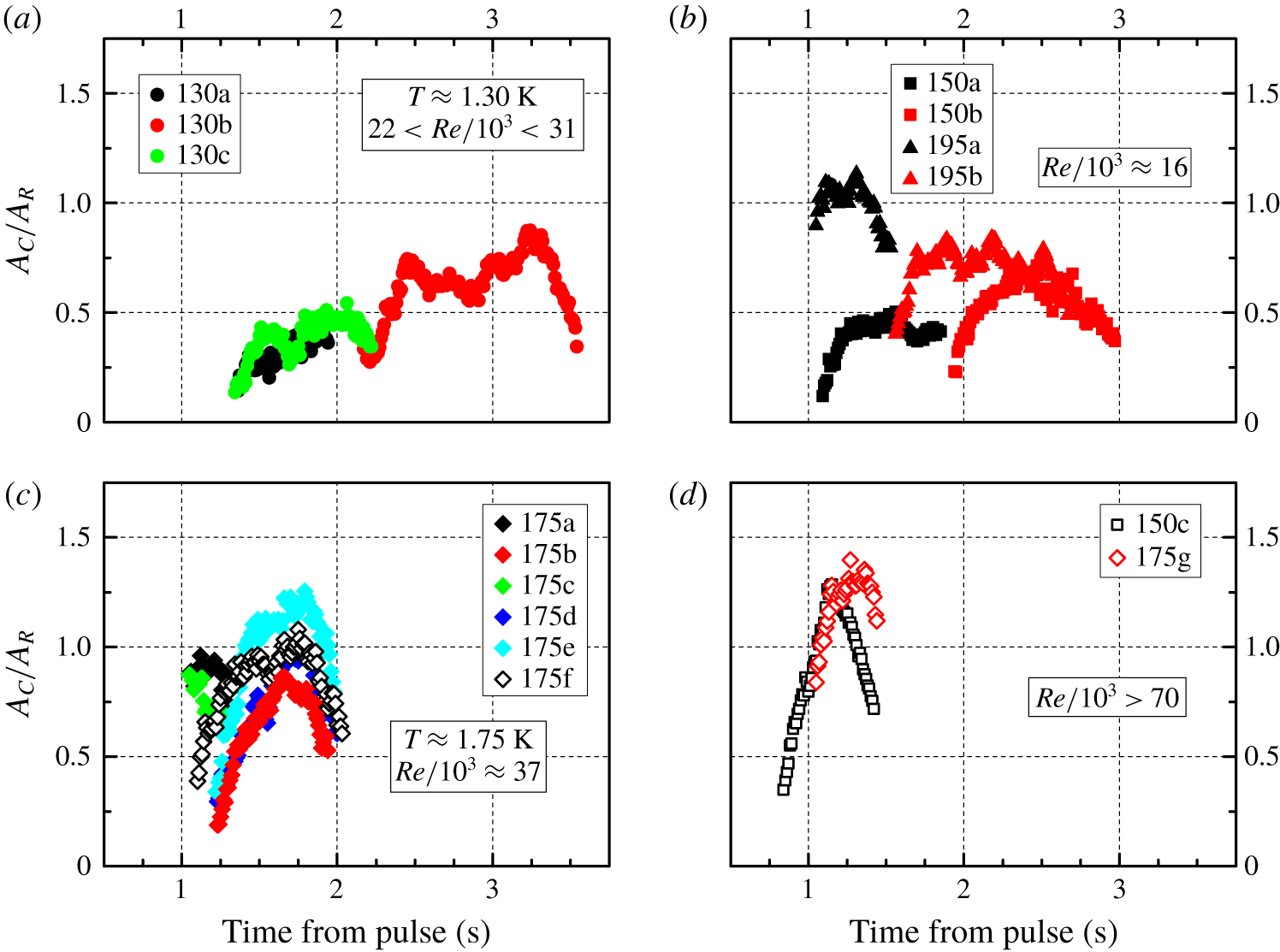
In order to get further insight into the relation between pseudovorticity and vorticity, we display in figure 13 the normalized ring area  $A_{C}/A_{R}$ as a function of the time elapsed from the end of the heat pulse, where
 $A_{C}$ is estimated by setting
 $\unicode[STIX]{x1D703}_{p}=1$ and
 $\unicode[STIX]{x1D703}_{n}=-1$ in (3.2) and
 $A_{R}=\unicode[STIX]{x03C0}R^{2}$. Note in passing that
 $A_{C}$ is of the same order as
 $A_{R}$, that is, the use of the ring radius
 $R$ as a first-order estimate of the ring size is here justified. More importantly, it is evident from figures 12 and 13 that the time dependence of
 $C/\unicode[STIX]{x1D6E4}_{0}$ closely resembles that of
 $A_{C}/A_{R}$. This outcome may indicate that the obtained values of pseudovorticity depend significantly on the number of tracked particles because, at relatively early and late times, fewer particles are used to quantify the ring strength, compared to when the fully formed ring is in the central part of the field of view. Note also that, as mentioned above, the ring core region is rarely tracked by our particles because the density of the latter is larger than that of the liquid.
Normalized ring area  $A_{C}/A_{R}$ as a function of the time elapsed from the end of the heat pulse; see the text for details. Symbols and panel description as in figure 7.

We can therefore say that, at present, we cannot directly access the flow vorticity and, consequently, the ring circulation. In order to address this issue one can envisage two routes. The flow vorticity could be experimentally measured by acoustic means, following, for example, Borner & Schmidt (Reference Borner, Schmidt, Meier and Obermeier1985), and/or relevant numerical simulations could be performed. The motion of viscous vortex rings could be computed numerically, in conditions similar to the experimental ones, and particles could be added later to the simulated flow fields. In this way one will likely be able to establish, for vortex rings, a quantitative relation between the Lagrangian pseudovorticity and the classical Eulerian vorticity. Attempts to follow both routes are currently under way and relevant results will be reported elsewhere.
In summary, from the above considerations, it appears that, in the case of macroscopic vortex rings, the use of the Lagrangian pseudovorticity leads to results consistent with the literature only when features such as the ring position and propagation velocity are considered, while the proposed technique is currently not adequate for investigating the fine structure of vortex rings, that is, the corresponding flow vorticity distribution.
3.4 Similarity theory
In order to further substantiate the previous claim we apply to our data the similarity theory developed by Glezer & Coles (Reference Glezer and Coles1990) for turbulent vortex rings. The theory assumes that these rings can be considered as self-similar objects, in certain conditions, and that their radius  $R$, position
 $y$ and velocity
 $v$ can be expressed in non-dimensional forms.


It is specifically postulated that, if viscous effects are neglected, the only relevant parameters that influence the ring motion are the fluid density  $\unicode[STIX]{x1D70C}$ and the hydrodynamic impulse
 $I$, which is assumed invariant, although measurements by Gan & Nickels (Reference Gan and Nickels2010) showed that, for turbulent rings,
 $I$ slowly decreases with time; see also the earlier work by Maxworthy (Reference Maxworthy1974).
In summary, from the theory it follows that
 $$\begin{eqnarray}R\sim (y-y_{0}),\end{eqnarray}$$
where  $y_{0}$ indicates a virtual space origin, and
 $$\begin{eqnarray}(y-y_{0})^{4}\sim (t-t_{0}),\end{eqnarray}$$
where  $t_{0}$ denotes a virtual time origin and
 $t$ is the time. Additionally, one can derive that
 $$\begin{eqnarray}c_{t}=v^{4/3}(t-t_{0}),\end{eqnarray}$$
where  $v$ indicates the ring propagation velocity,
 $$\begin{eqnarray}c_{y}=v^{1/3}(y-y_{0})\end{eqnarray}$$
and
 $$\begin{eqnarray}c_{R}=v^{1/3}R;\end{eqnarray}$$
see, for example, Gan & Nickels (Reference Gan and Nickels2010) for further details on the derivation of these rules.
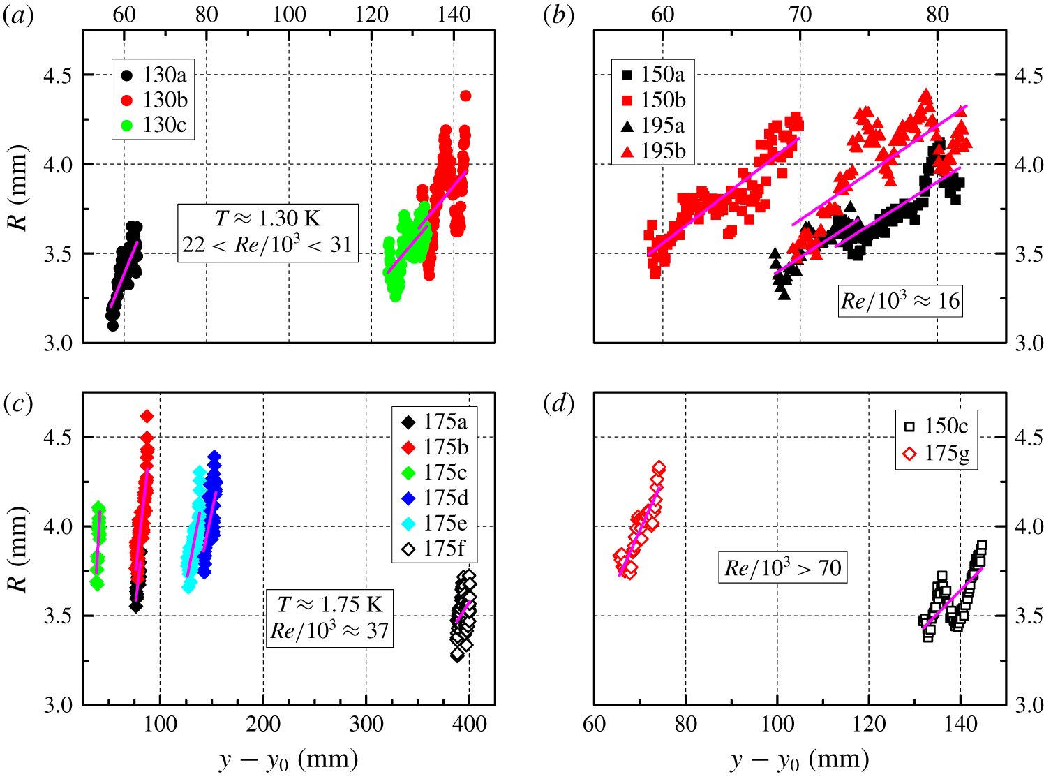
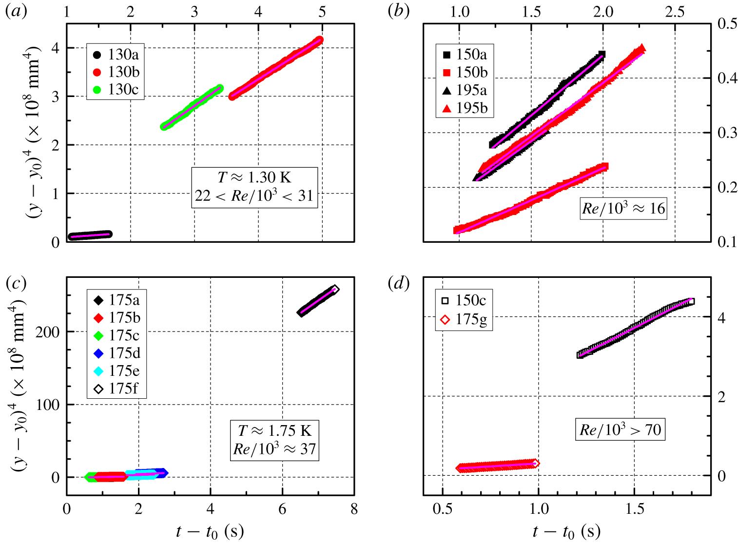
The experimentally obtained dependence of the ring radius  $R$ on the position
 $y$, displayed in figures 7 and 8, was employed to estimate the virtual origin
 $y_{0}$, equation (3.3), by using adequate linear fits, and, in a similar fashion, by employing the obtained values of
 $y_{0}$, we estimated
 $t_{0}$, equation (3.4).
From the corresponding results, shown in figures 14 and 15, it is evident that, for the present experimental data, the direct proportionality between  $(y-y_{0})^{4}$ and
 $(t-t_{0})$ is neater than that between
 $R$ and
 $(y-y_{0})$. Therefore, this outcome also suggests that the parameter
 $\unicode[STIX]{x1D703}$ does not seem adequate for estimating accurately the spatial extension of vortex rings, at least in the range of investigated parameters.


We also calculated the similarity constants  $c_{t}$,
 $c_{y}$ and
 $c_{R}$, by using the ring velocity
 $v$, plotted in figure 9 as a function of the time elapsed from the end of the heat pulse. Note that the values of these constants are expected to depend on a particular realization of the flow, while the ratios
 $c_{y}/c_{t}$ and
 $c_{R}/c_{t}$ should be universal constants.
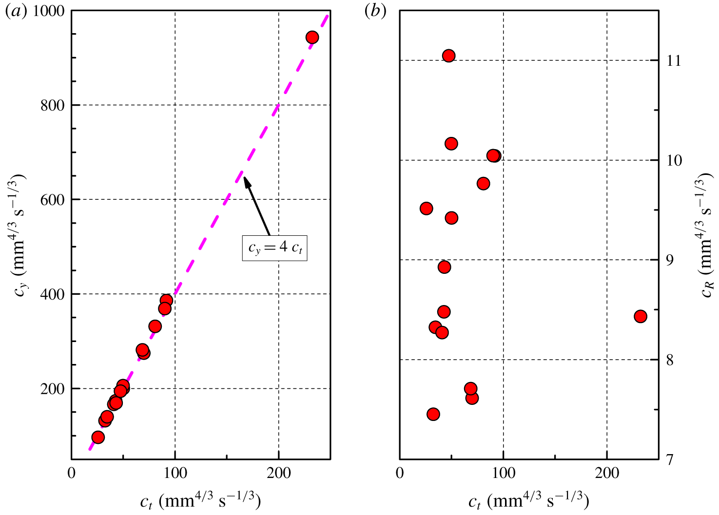
(a) Similarity constant  $c_{y}$, equation (3.6), as a function of
 $c_{t}$, equation (3.5); the dashed magenta line indicates the theoretical expectation (Glezer & Coles Reference Glezer and Coles1990; Gan & Nickels Reference Gan and Nickels2010). (b) Similarity constant
 $c_{R}$, equation (3.7), as a function of
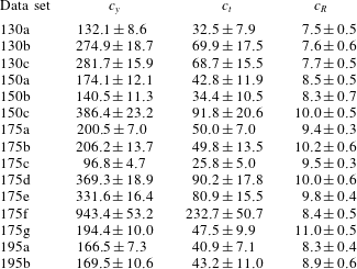
 $c_{t}$. Only mean values are plotted, for the sake of clarity, see table 3 for corresponding mean values and standard deviations.


As is apparent from table 3 and figure 16(a), the ratio  $c_{y}/c_{t}$ is, for the present data sets, approximately equal to 4, which is the value expected from the similarity theory (Glezer & Coles Reference Glezer and Coles1990; Gan & Nickels Reference Gan and Nickels2010). This indicates that our vortex rings behave as if they were turbulent vortex rings moving in a viscous fluid, at least in the direction of ring propagation. Additionally, this outcome confirms that the ring vertical motion is adequately tracked by the pseudovorticity method employed in this study, although, as mentioned above, the same cannot be said for the radial direction.
Indeed, the ratio  $c_{R}/c_{t}$, which can be linked to the ring self-similar radial evolution, does not appear to be constant for the present data sets, see table 3 and figure 16(b), that is, it experiences larger relative variations in comparison with those of
 $c_{y}/c_{t}$. The outcome could also be related to the ring trajectory dispersion and/or to the occurrence of azimuthal waves, which we cannot currently access experimentally, but it is mostly likely due to the already mentioned limitations of the used experimental technique.
Nevertheless, it is remarkable that, as shown in table 3, the standard deviations of the estimated similarity constants are appreciably smaller than the corresponding mean values, that is, for each data set,  $c_{y}$,
 $c_{t}$ and
 $c_{R}$ seem indeed to be constant, at least in the range of investigated parameters. However, it is currently not clear why the constants
 $c_{y}$ and
 $c_{t}$ for the data set 175f are much larger than for the others, but the result could be related to the smaller pulse duration in this case, remarked above in the discussion on the ring velocity.
Note also that, at present, we cannot estimate the ring impulse  $I$ because, as mentioned above, a general, quantitative relation between the Lagrangian pseudovorticity and the Eulerian vorticity is yet to be established, although the obtained
 $c_{R}/c_{t}$ trend could also be influenced by the fact that
 $I$ is not exactly an invariant of the studied motion (Maxworthy Reference Maxworthy1974; Gan & Nickels Reference Gan and Nickels2010).
4 Conclusions
We experimentally investigated the early development of macroscopic vortex rings in superfluid 4He, where early means at distances between 1 and 6 times the nozzle diameter. The rings were generated thermally, by applying a short heat pulse, with temperatures ranging from 1.28 to 1.95 K, in the two-fluid regime of He II, when the fluid viscosity cannot be neglected. The applied heat fluxes were between  $35$ to
 $450$ mW cm
 $^{-2}$, resulting in Reynolds numbers of the order of
 $10^{4}$.
The rings were identified and tracked by using the concept of Lagrangian pseudovorticity, recently introduced to quantify the strength of large vortical structures in the absence of Eulerian data (Duda et al. Reference Duda, Švančara, La Mantia, Rotter and Skrbek2015, Reference Duda, La Mantia and Skrbek2017). We found that the ring features can be quantitatively assessed by using this method and can therefore be used to perform relevant comparisons.
Our aim was indeed to make a significant contribution to the active line of scientific enquiry focusing on the study of similarities and differences between classical and quantum flows. We found that, in the range of investigated parameters, our rings behave as if they were turbulent vortex rings moving in a viscous fluid, at least in the direction of ring propagation. This claim is mainly based on the remarkable agreement between our experimental results and the similarity theory developed by Glezer & Coles (Reference Glezer and Coles1990) for turbulent vortex rings. Additionally, the observed ring features do not seem to depend significantly on fluid temperature and Reynolds number.
The results therefore reinforce the view that, at scales larger than the mean distance between quantized vortices, quantum flows may display distinctive classical-like features, as discussed in previous works on different types of He II flows (see, for example, Švančara & La Mantia Reference Švančara and La Mantia2017, Reference Švančara and La Mantia2019), that is, the observed behaviour does not appear to be strongly influenced by the flow generation mechanism, at least in the range of investigated parameters. On the other hand, the reason why superfluid 4He behaves in such a way is still largely unknown and further studies are needed to address the problem.
A possible route for future investigations could start from the experimental results recently reported by Švančara & La Mantia (Reference Švančara and La Mantia2019), which clearly show that the mechanisms of energy transport in turbulent flows of He II are strikingly different from those occurring in similar flows of viscous fluids. In other words, by studying the late development of macroscopic vortex rings in superfluid 4He, where late means at distances from the nozzle appreciably larger than in the present case, one might be able to find distinctive large-scale quantum features.
Another research route, which is potentially not only relevant to quantum turbulence, could focus on clarifying the relation between the Lagrangian pseudovorticity and the Eulerian vorticity. As mentioned above, this could be achieved by using numerical simulations and/or by directly measuring the flow vorticity, for example, by acoustic means, following Borner & Schmidt (Reference Borner, Schmidt, Meier and Obermeier1985).
In summary, our work on macroscopic vortex rings in He II shows that the study of turbulent flows of superfluid 4He is not only interesting in its own right, but that it can also contribute to our current understanding of fluid turbulence in general.
Acknowledgements
We thank A. Andrýsková, P. Hrubcová, O. Outrata, J. Hron and B. Vejr for valuable help. The support of the Czech Science Foundation (GAČR) under grant no. 19-00939S is acknowledged.
Declaration of interests
The authors report no conflict of interest.