1 Introduction
1.1 Background
Direct numerical simulation (DNS) of particle-, bubble- and droplet-laden turbulent flows has been used to explain physical mechanisms occurring in such flows, and spectral analysis has been an important tool in understanding the physics of such flows (Elghobashi Reference Elghobashi2019). For example, Elghobashi & Truesdell (Reference Elghobashi and Truesdell1993) simulated decaying homogeneous isotropic turbulence interacting with dispersed solid particles of diameter less than the Kolmogorov length scale. They found that the particles caused an increase in spectral turbulence kinetic energy (TKE) at high wavenumbers. Ferrante & Elghobashi (Reference Ferrante and Elghobashi2003) extended this analysis to find that the energy spectrum is affected by a spectral two-way coupling function due to fluid–particle drag interaction, which results in an increase of energy at high wavenumbers for a range of sub-Kolmogorov particles with Stokes number between
 $0.1$
and
 $5$
.
Because the particles of these simulations were smaller than the Kolmogorov length scale of turbulence and represented by infinitesimal points rather than finite volumes, the authors computed the energy spectra in the traditional way, that is, using the Fourier transform across the entire domain. Spectral analysis becomes more difficult for particles of Taylor length-scale size as studied by Lucci, Ferrante & Elghobashi (Reference Lucci, Ferrante and Elghobashi2010). These larger particles have a finite volume in the computational domain, so the velocity field becomes discontinuous at the particle–fluid interfaces, and these discontinuities manifest themselves as oscillations in the energy spectra (Lucci et al. Reference Lucci, Ferrante and Elghobashi2010, figure 35). These oscillations appear because the energy spectrum is defined using the Fourier transform, which uses infinite sinusoidal waves to represent functions in the frequency domain. Such basis functions cannot easily capture discontinuities. Lucci et al. (Reference Lucci, Ferrante and Elghobashi2010) therefore use an alternative definition of the energy spectrum. Instead of computing the spectrum using the Eulerian velocity field, they track a large number of fluid points and use their velocity to compute a Lagrangian TKE spectrum. While this approach is definitely valuable, it adds the computational costs of computing, writing and storing the fluid points’ velocity during the simulations.
A related area of research is that of experimental ‘pseudoturbulence’ generated by rising bubbles (Risso Reference Risso2018). Hot-wire anemometers also produce discontinuous data due to the popping of bubbles by the probe. A variety of methods has been used to overcome the artefacts introduced by the discontinuities when producing energy spectra such as interpolation, selective sampling in the Fourier transform and fitting of Gaussian curves. However, these techniques were derived for the one-dimensional velocity time series produced by the anemometer, so they would not be easily applicable to our three-dimensional velocity fields. Most importantly, these techniques involve modifications of the velocity field, while we propose a way to generate TKE spectra without artificially modifying the velocity field at all.
1.2 Motivation
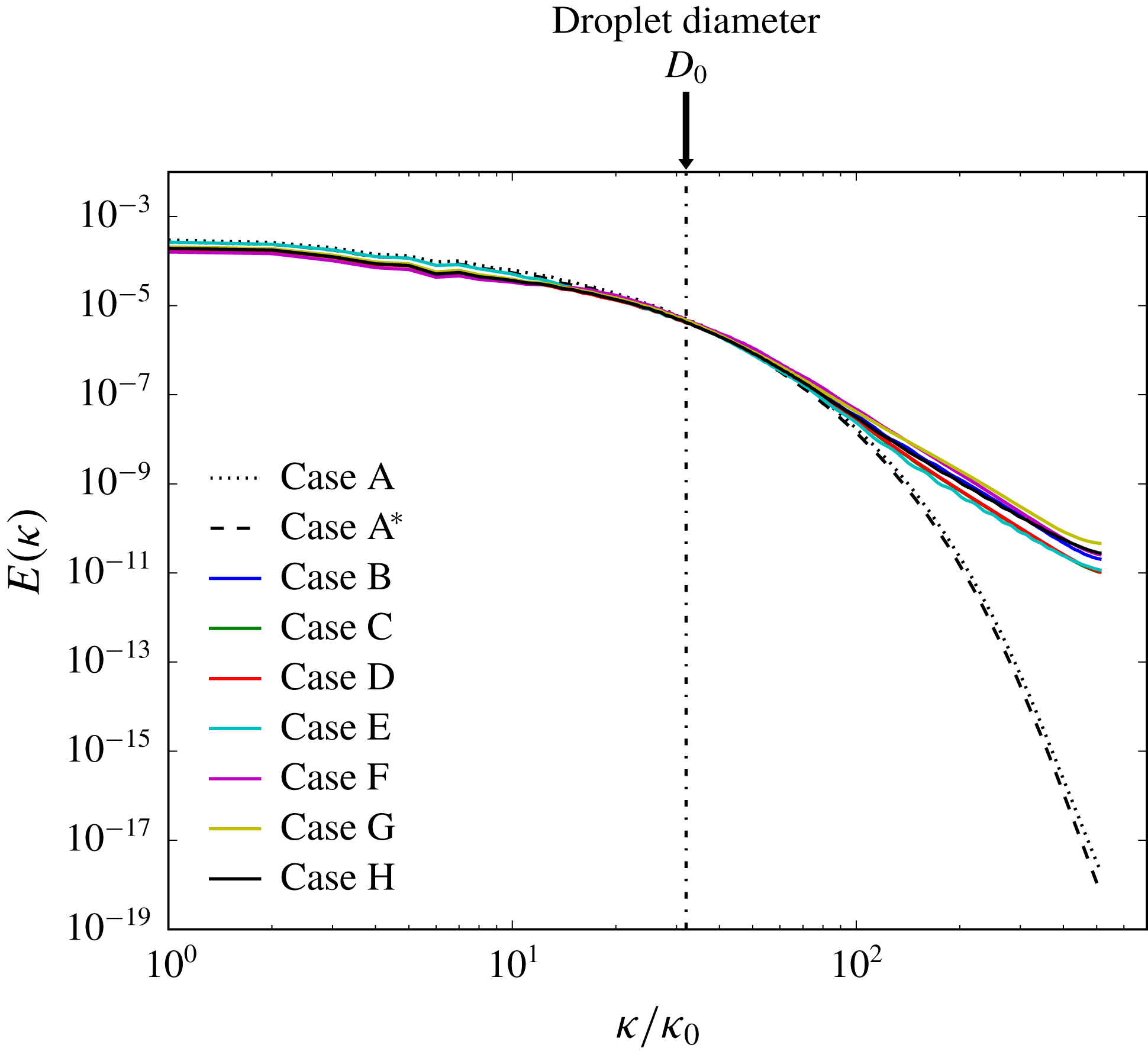
Fourier spectra of TKE for the DNS cases of Dodd & Ferrante (Reference Dodd and Ferrante2016). Dashed lines represent droplet-free cases and solid lines droplet-laden cases.

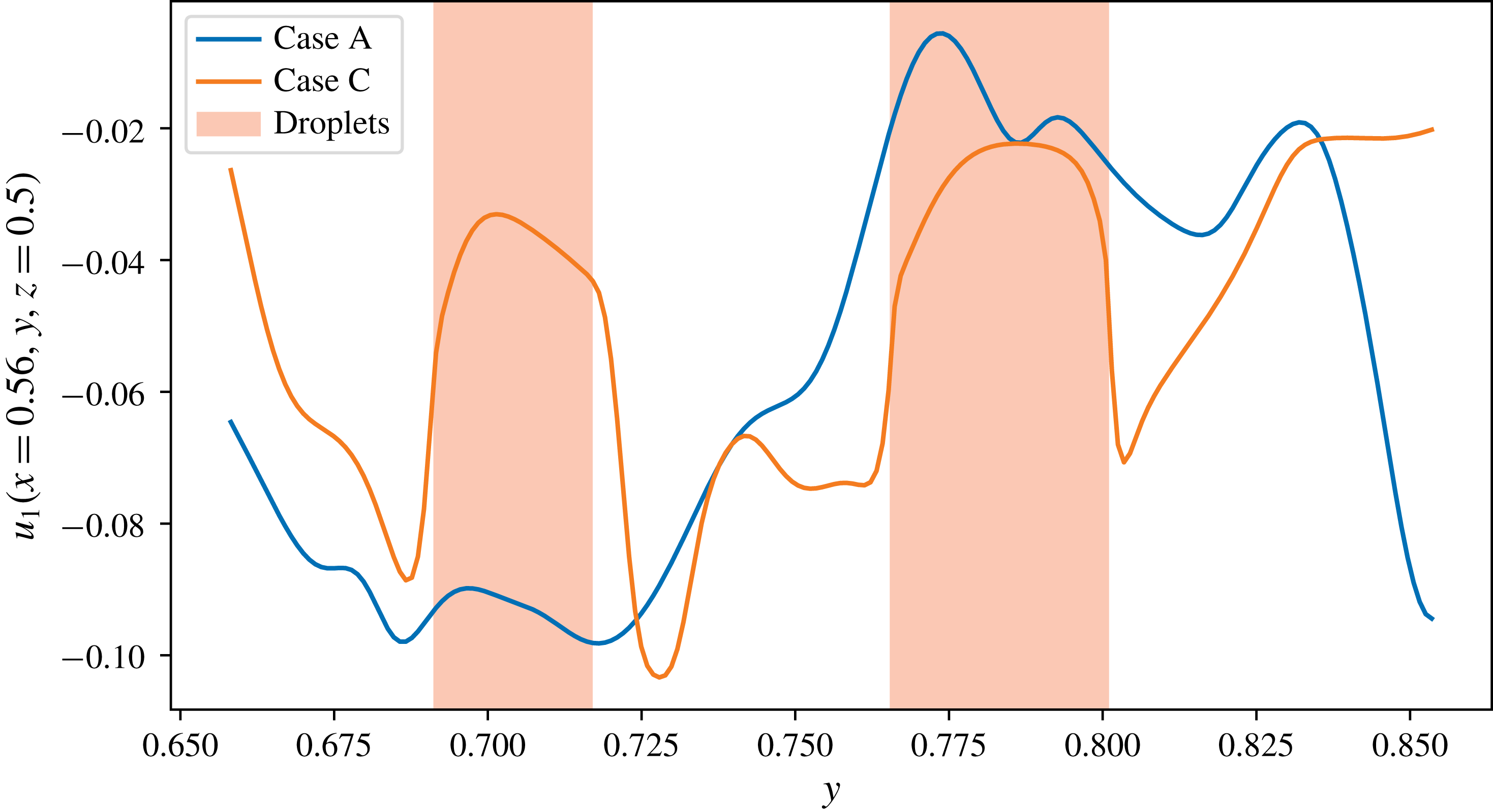
Velocity profiles along a line in the domain show sharp jumps at the interfaces for droplet-laden case C.

We are interested in the analysis of energy spectra for homogeneous isotropic turbulence laden with droplets of Taylor length-scale size. These finite-sized droplets present similar issues as the particles of Lucci et al. (Reference Lucci, Ferrante and Elghobashi2010). Figure 1 shows the Fourier energy spectra of droplet-laden turbulence studied via DNS by Dodd & Ferrante (Reference Dodd and Ferrante2016). In that figure, note the general differences between the droplet-free and droplet-laden cases: introduction of the droplets causes energy at low wavenumbers to decrease, energy at high wavenumbers to increase and the spectra to oscillate slightly at high wavenumbers. The last feature is a result of the Fourier transform’s inability to handle sharp changes at droplet interfaces.
Figure 2 shows an example of how the droplets exhibit sharp changes in velocity around their interfaces with the carrier fluid. Though we are dealing with deformable droplets and not particles, even if the shear is continuous at the interface, the velocity gradient at the interface is still discontinuous (Dodd & Ferrante Reference Dodd and Ferrante2016, figure 30); thus, high-frequency modes are enhanced when taking the Fourier transform. This has led us to question whether the introduction of droplets actually causes the carrier fluid to contain more energy at high wavenumbers. Also, Maxey (Reference Maxey2017) suggests providing a closer analysis of the energy spectrum in his review of Dodd & Ferrante (Reference Dodd and Ferrante2016). Furthermore, our interest in the droplets’ effect on the energy spectrum is to help improve subgrid-scale models for large-eddy simulation (LES) of multiphase turbulent flows.
1.3 Our approach
Instead of using the Fourier transform to compute the energy spectrum, we use the wavelet-transform approach as described by Meneveau (Reference Meneveau1991). We extend his wavelet formulation to multiphase incompressible turbulence. A wavelet is typically an oscillating function with compact support. The wavelet transform is used to represent a function in a basis of wavelets. The primary advantage of the wavelet transform for this application is that it preserves spatial information, making it a natural choice for a two-fluid flow. Besides restricting effects of non-smoothness locally, the spatial information allows us to decompose the spectrum as explained in § 2.5.
As the computation of non-homogeneous and multiphase turbulent flows becomes increasingly tractable, wavelet and wavelet-like approaches have been applied in a few recent studies. For example, wavelets have been used to analyse particle-laden flows (Bassenne, Moin & Urzay Reference Bassenne, Moin and Urzay2018) and turbulent combustion (Kim et al. Reference Kim, Bassenne, Towery, Hamlington, Poludnenko and Urzay2018). A similar approach was used to compute spectra on non-periodic domains by using spatial filtering with a customized non-wavelet basis (Sadek & Aluie Reference Sadek and Aluie2018).
1.4 Flow description
Dodd & Ferrante (Reference Dodd and Ferrante2016) performed DNS of 3130 finite-size, non-evaporating droplets of diameter approximately equal to the Taylor length scale and with 5 % droplet volume fraction in incompressible decaying isotropic turbulence at initial Taylor-scale Reynolds number
 $\mathit{Re}_{\unicode[STIX]{x1D706}}=83$
and zero gravity. They numerically solved the incompressible Navier–Stokes equations for two immiscible fluids (Dodd & Ferrante Reference Dodd and Ferrante2014). Following their nomenclature, also adopted herein,
 $\boldsymbol{u}(\boldsymbol{x},t)$
is the velocity field,
 $p(\boldsymbol{x},t)$
is the pressure,
 $\unicode[STIX]{x1D70C}(\boldsymbol{x},t)$
is the density,
 $\unicode[STIX]{x1D707}(\boldsymbol{x},t)$
is the dynamic viscosity,
 $\mathit{Re}$
is the Reynolds number,
 $\mathit{We}$
is the Weber number and
 $\boldsymbol{f}_{\unicode[STIX]{x1D70E}}(\boldsymbol{x},t)$
is the force due to surface tension;
 $\unicode[STIX]{x1D70C}$
and
 $\unicode[STIX]{x1D707}$
are constant in each phase, taking values
 $\unicode[STIX]{x1D70C}_{c}$
and
 $\unicode[STIX]{x1D707}_{c}$
in the carrier fluid and
 $\unicode[STIX]{x1D70C}_{d}$
and
 $\unicode[STIX]{x1D707}_{d}$
in the droplets. The physical flow and droplet parameters of the DNS cases are given in tables 1 and 2, respectively, of Dodd & Ferrante (Reference Dodd and Ferrante2016). In particular, the initial droplet diameter
 $D$
satisfies
 $D/\unicode[STIX]{x0394}x=32$
, where
 $\unicode[STIX]{x0394}x$
is the grid size, and
 $D/\unicode[STIX]{x1D702}=20$
, where
 $\unicode[STIX]{x1D702}$
is the Kolmogorov length scale at the time the droplets are released (
 $t=1$
). Case A is the reference droplet-free case. In the droplet-laden cases (B–H), they varied one of the following three parameters: the droplet Weber number based on the root mean square velocity of turbulence (
 $0.1\leqslant \mathit{We}_{rms}\leqslant 5$
) in cases B, C and D; the droplet to carrier-fluid density ratio (
 $1\leqslant \unicode[STIX]{x1D70C}_{d}/\unicode[STIX]{x1D70C}_{c}\leqslant 100$
) in cases E, C and F; or the droplet to carrier-fluid viscosity ratio (
 $1\leqslant \unicode[STIX]{x1D707}_{d}/\unicode[STIX]{x1D707}_{c}\leqslant 100$
) in cases G, C and H. In § 3, we present the wavelet-spectral analysis of all cases A–H at non-dimensional time
 $t=3.5$
.
2 Mathematical description
2.1 Discrete wavelet transform
The basic idea behind the discrete wavelet transform (DWT) is to represent a function using self-similar basis functions, which are dilated and translated in the space of the data set. These basis functions are made orthonormal by using a logarithmic spacing of scales. In the following, we use a notation similar to that of Meneveau (Reference Meneveau1991).
If
 $g[n]$
is our ‘mother’ wavelet, where
 $g$
is a discrete function sampled at
 $x_{n}=n\unicode[STIX]{x0394}x$
with an integer
 $n$
and the grid spacing
 $\unicode[STIX]{x0394}x$
, the basis functions take the form
 $$\begin{eqnarray}\displaystyle g^{(m)}[n-2^{m}l]={\displaystyle \frac{1}{2^{m/2}}}g\left[{\displaystyle \frac{n-2^{m}l}{2^{m}}}\right], & & \displaystyle\end{eqnarray}$$
where
 $m$
is the wavelet-scale index, which determines the amount of dilation, and
 $l$
determines the translation away from the initial position. Associated with the wavelet functions is also a smoothing function
 $h[n]$
that is dilated and translated in the same way. In three dimensions, we must use products of
 $g^{(m)}$
and
 $h^{(m)}$
in order to represent our data with dilations in every possible combination of directions. In total, there are seven possible combinations: one volumetric dilation, i.e. one in all three directions at once; three planar dilations, i.e. one for each plane (
 $x$
–
 $y$
,
 $y$
–
 $z$
and
 $x$
–
 $z$
); and three linear dilations, i.e. one in each direction (
 $x$
,
 $y$
and
 $z$
). Using the index
 $q$
to distinguish between these seven combinations, we thus define a three-dimensional basis function
 $g^{(m,q)}[\boldsymbol{n}-2^{m}\boldsymbol{l}]$
(Meneveau Reference Meneveau1991, equation (30)), where
 $\boldsymbol{n}$
and
 $\boldsymbol{l}$
are the three-dimensional counterparts to the indices
 $n$
and
 $l$
.
With our basis functions defined, we may represent each component of velocity as
 $$\begin{eqnarray}\displaystyle u_{i}[\boldsymbol{n}]=\mathop{\sum }_{m=1}^{M}\mathop{\sum }_{q=1}^{7}\mathop{\sum }_{\boldsymbol{l}\in {\mathcal{D}}^{(m)}}w_{i}^{(m,q)}[\boldsymbol{l}]g^{(m,q)}[\boldsymbol{n}-2^{m}\boldsymbol{l}],\quad i=1,2,3, & & \displaystyle\end{eqnarray}$$
where the wavelet coefficients are given by
 $$\begin{eqnarray}\displaystyle w_{i}^{(m,q)}[\boldsymbol{l}]=\mathop{\sum }_{\boldsymbol{n}\in {\mathcal{D}}}u_{i}[\boldsymbol{n}]g^{(m,q)}[\boldsymbol{n}-2^{m}\boldsymbol{l}]. & & \displaystyle\end{eqnarray}$$
Here
 ${\mathcal{D}}=\{1,\ldots ,N\}^{3}$
is the set of indices on which the velocity field is defined (in our case
 $N=1024$
) and
 ${\mathcal{D}}^{(m)}=\{1,\ldots ,N/{2^{m}\}}^{3}$
is the set of indices on which the scale-
 $m$
wavelet coefficients are defined.
 $M=\log _{2}N$
is the number of scales that we can use (so in our case
 $M=10$
). The DWT conserves energy because
 $$\begin{eqnarray}\displaystyle \mathop{\sum }_{i=1}^{3}\mathop{\sum }_{\boldsymbol{n}\in {\mathcal{D}}}u_{i}[\boldsymbol{n}]^{2}=\mathop{\sum }_{i=1}^{3}\mathop{\sum }_{m=1}^{M}\mathop{\sum }_{q=1}^{7}\mathop{\sum }_{\boldsymbol{l}\in {\mathcal{D}}^{(m)}}w_{i}^{(m,q)}[\boldsymbol{l}]^{2}. & & \displaystyle\end{eqnarray}$$
2.2 Wavelet spectrum
The wavenumber
 $k_{m}$
is related to the wavelet scale
 $m$
by
 $$\begin{eqnarray}\displaystyle k_{m}={\displaystyle \frac{2\unicode[STIX]{x03C0}}{2^{m}\unicode[STIX]{x0394}x}}, & & \displaystyle\end{eqnarray}$$
where
 $\unicode[STIX]{x0394}x={\mathcal{L}}/N$
is the size of the spatial discretization of our DNS data with
 ${\mathcal{L}}$
the non-dimensional side length of the cubical domain and
 $N$
the number of grid points per domain (here
 $\unicode[STIX]{x0394}x=1/1024$
). The largest scale corresponds to
 $m=M$
, so using (2.5), the minimum wavelet wavenumber is
 $k_{min}=k_{M}=2\unicode[STIX]{x03C0}$
.
The wavelet spectrum is then given by
 $$\begin{eqnarray}\displaystyle \widetilde{E}(k_{m})=C_{m}\mathop{\sum }_{i=1}^{3}\mathop{\left\langle \frac{1}{2}\mathop{\sum }_{q=1}^{7}w_{i}^{(m,q)}[\boldsymbol{l}]^{2}\right\rangle }\nolimits_{\boldsymbol{l}\in {\mathcal{D}}^{(m)}}, & & \displaystyle\end{eqnarray}$$
where
 $\langle \cdot \rangle _{\boldsymbol{l}\in {\mathcal{D}}^{(m)}}$
denotes the average over
 $\boldsymbol{l}\in {\mathcal{D}}^{(m)}$
, and
 $C_{m}=\unicode[STIX]{x0394}x/[2\unicode[STIX]{x03C0}(\log 2)2^{2m}]$
is included to scale the spectrum so that
 $\widetilde{E}(k_{m})$
represents the energy spectrum per unit wavenumber.
2.3 Choice of wavelet
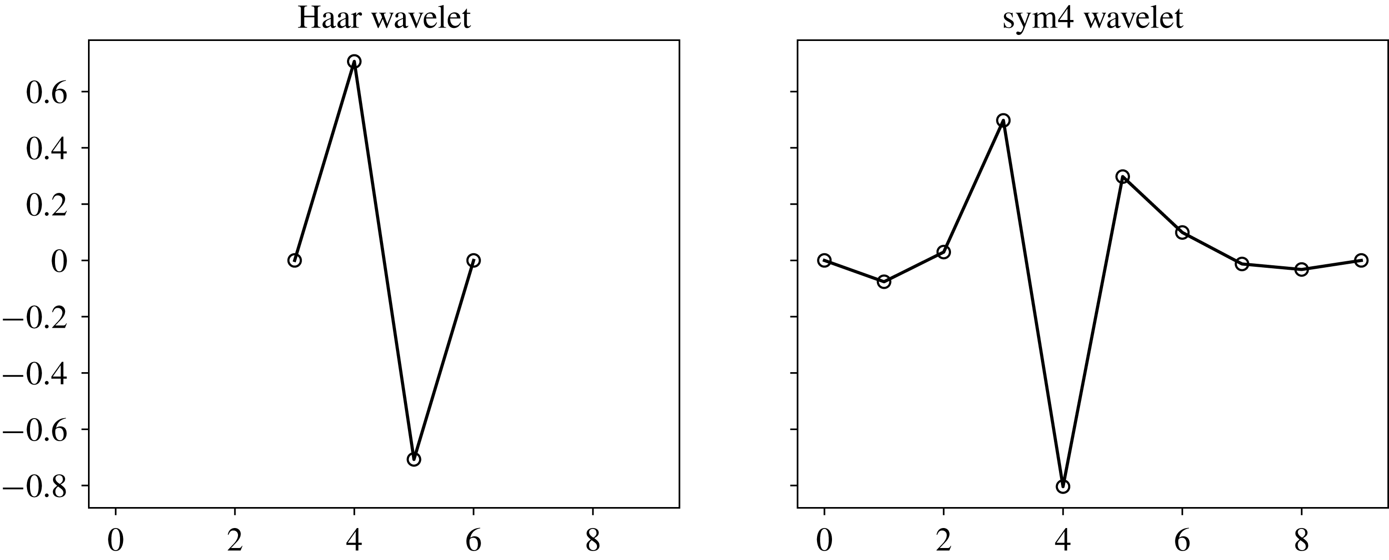
Comparison of the Haar wavelet and the sym4 wavelet used in this study.

A comparison of energy spectra produced with various wavelets is given by Perrier, Philipovitch & Basevant (Reference Perrier, Philipovitch and Basevant1995). The choice of wavelet is also discussed by Meneveau (Reference Meneveau1991, § 5.3). We have used both the Haar and sym4 wavelets to analyse our data. Both are common options and their definitions can be found in the PyWavelets DWT package (Lee et al. Reference Lee, Gommers, Waselewski, Wohlfahrt and O’Leary2019; PyWavelets 2018). The Haar wavelet has the advantage of being simple and easy to compute. Because it requires fewer points to calculate than other wavelet basis functions (figure 3), it also allows for more spatial resolution, which would be desirable when we decompose the spectrum. However, since it uses fewer points than other functions, a single basis function encodes less information. As a result, more small-scale wavelet coefficients are needed to represent the flow field in the wavelet basis, so the Haar wavelet produces relatively flat spectra. On the other hand, the sym4 wavelet produces wavelet spectra more closely resembling the respective Fourier spectra (in that they decay at the high wavenumbers) because its basis function oscillates more in space than the Haar wavelet, more closely resembling a truncated sine function of the Fourier transform. This property is important in analysing the wavelet spectra in comparison to the Fourier spectra, and so sym4 is the wavelet we adopted in this study.
2.4 Evolution of wavelet spectrum
The DWT of the momentum equation (2.1b) of Dodd & Ferrante (Reference Dodd and Ferrante2016) gives
 $$\begin{eqnarray}\displaystyle {\displaystyle \frac{\unicode[STIX]{x2202}}{\unicode[STIX]{x2202}t}}w_{i}^{(m,q)}[\boldsymbol{l}] & = & \displaystyle -\left\{u_{j}{\displaystyle \frac{\unicode[STIX]{x2202}u_{i}}{\unicode[STIX]{x2202}x_{j}}}+\frac{1}{\unicode[STIX]{x1D70C}}{\displaystyle \frac{\unicode[STIX]{x2202}p}{\unicode[STIX]{x2202}x_{i}}}\right\}^{(m,q)}[\boldsymbol{l}]\nonumber\\ \displaystyle & & \displaystyle +\,\left\{\frac{1}{\unicode[STIX]{x1D70C}\mathit{Re}}{\displaystyle \frac{\unicode[STIX]{x2202}}{\unicode[STIX]{x2202}x_{j}}}\left(\unicode[STIX]{x1D707}\left({\displaystyle \frac{\unicode[STIX]{x2202}u_{i}}{\unicode[STIX]{x2202}x_{j}}}+{\displaystyle \frac{\unicode[STIX]{x2202}u_{j}}{\unicode[STIX]{x2202}x_{i}}}\right)\right)\right\}^{(m,q)}[\boldsymbol{l}]+\left\{\frac{1}{\unicode[STIX]{x1D70C}\mathit{We}}(f_{\unicode[STIX]{x1D70E}})_{i}\right\}^{(m,q)}[\boldsymbol{l}].\quad\end{eqnarray}$$
We use the convention
 $\{\cdot \}^{(m,q)}[\boldsymbol{l}]$
to denote the DWT, and we are able to apply the DWT term-by-term since it is a linear operator. Then, by multiplying each term of (2.7) by
 $w_{i}^{(m,q)}[\boldsymbol{l}]$
and by applying the chain rule in reverse to the left-hand side of the resulting equation,
 $$\begin{eqnarray}\displaystyle w_{i}^{(m,q)}[\boldsymbol{l}]{\displaystyle \frac{\unicode[STIX]{x2202}}{\unicode[STIX]{x2202}t}}w_{i}^{(m,q)}[\boldsymbol{l}]={\displaystyle \frac{\unicode[STIX]{x2202}}{\unicode[STIX]{x2202}t}}\left(\frac{1}{2}w_{i}^{(m,q)}[\boldsymbol{l}]^{2}\right), & & \displaystyle\end{eqnarray}$$
we get
 $$\begin{eqnarray}\displaystyle & & \displaystyle {\displaystyle \frac{\unicode[STIX]{x2202}}{\unicode[STIX]{x2202}t}}\left(\frac{1}{2}w_{i}^{(m,q)}[\boldsymbol{l}]^{2}\right)=-w_{i}^{(m,q)}[\boldsymbol{l}]\left\{u_{j}{\displaystyle \frac{\unicode[STIX]{x2202}u_{i}}{\unicode[STIX]{x2202}x_{j}}}+\frac{1}{\unicode[STIX]{x1D70C}}{\displaystyle \frac{\unicode[STIX]{x2202}p}{\unicode[STIX]{x2202}x_{i}}}\right\}^{(m,q)}[\boldsymbol{l}]\nonumber\\ \displaystyle & & \displaystyle \quad +\,w_{i}^{(m,q)}[\boldsymbol{l}]\left\{\frac{1}{\unicode[STIX]{x1D70C}\mathit{Re}}{\displaystyle \frac{\unicode[STIX]{x2202}}{\unicode[STIX]{x2202}x_{j}}}\left(\unicode[STIX]{x1D707}\left({\displaystyle \frac{\unicode[STIX]{x2202}u_{i}}{\unicode[STIX]{x2202}x_{j}}}+{\displaystyle \frac{\unicode[STIX]{x2202}u_{j}}{\unicode[STIX]{x2202}x_{i}}}\right)\right)\right\}^{(m,q)}[\boldsymbol{l}]+w_{i}^{(m,q)}[\boldsymbol{l}]\left\{\frac{1}{\unicode[STIX]{x1D70C}\mathit{We}}(f_{\unicode[STIX]{x1D70E}})_{i}\right\}^{(m,q)}[\boldsymbol{l}].\nonumber\\ \displaystyle & & \displaystyle\end{eqnarray}$$
Summing each term of (2.9) over
 $q$
and
 $i$
and averaging the resulting equation over all scale-
 $m$
wavelet coefficients gives us
 $$\begin{eqnarray}\displaystyle {\displaystyle \frac{\unicode[STIX]{x2202}}{\unicode[STIX]{x2202}t}}\widetilde{E}(k_{m})=\widetilde{T}(k_{m})-\widetilde{V}(k_{m})+\widetilde{S}(k_{m}). & & \displaystyle\end{eqnarray}$$
Here,
 $\widetilde{E}(k_{m})$
is the wavelet energy spectrum defined in (2.6), and the terms on the right-hand side of (2.10) are defined by
 $$\begin{eqnarray}\displaystyle & \displaystyle \widetilde{T}(k_{m})=-C_{m}\mathop{\sum }_{i=1}^{3}\mathop{\left\langle \mathop{\sum }_{q=1}^{7}w_{i}^{(m,q)}[\boldsymbol{l}]\left\{u_{j}{\displaystyle \frac{\unicode[STIX]{x2202}u_{i}}{\unicode[STIX]{x2202}x_{j}}}+\frac{1}{\unicode[STIX]{x1D70C}}{\displaystyle \frac{\unicode[STIX]{x2202}p}{\unicode[STIX]{x2202}x_{i}}}\right\}^{(m,q)}[\boldsymbol{l}]\right\rangle }\nolimits_{\boldsymbol{l}\in {\mathcal{D}}^{(m)}}, & \displaystyle\end{eqnarray}$$
 $$\begin{eqnarray}\displaystyle & \displaystyle \widetilde{V}(k_{m})=-C_{m}\mathop{\sum }_{i=1}^{3}\mathop{\left\langle \mathop{\sum }_{q=1}^{7}w_{i}^{(m,q)}[\boldsymbol{l}]\left\{\frac{1}{\unicode[STIX]{x1D70C}\mathit{Re}}{\displaystyle \frac{\unicode[STIX]{x2202}}{\unicode[STIX]{x2202}x_{j}}}\left(\unicode[STIX]{x1D707}\left({\displaystyle \frac{\unicode[STIX]{x2202}u_{i}}{\unicode[STIX]{x2202}x_{j}}}+{\displaystyle \frac{\unicode[STIX]{x2202}u_{j}}{\unicode[STIX]{x2202}x_{i}}}\right)\right)\right\}^{(m,q)}[\boldsymbol{l}]\right\rangle }\nolimits_{\boldsymbol{l}\in {\mathcal{D}}^{(m)}},\qquad & \displaystyle\end{eqnarray}$$
 $$\begin{eqnarray}\displaystyle & \displaystyle \widetilde{S}(k_{m})=C_{m}\mathop{\sum }_{i=1}^{3}\mathop{\left\langle \mathop{\sum }_{q=1}^{7}w_{i}^{(m,q)}[\boldsymbol{l}]\left\{\frac{1}{\unicode[STIX]{x1D70C}\mathit{We}}(f_{\unicode[STIX]{x1D70E}})_{i}\right\}^{(m,q)}[\boldsymbol{l}]\right\rangle }\nolimits_{\boldsymbol{l}\in {\mathcal{D}}^{(m)}}, & \displaystyle\end{eqnarray}$$
where
 $\widetilde{T}(k_{m})$
is the energy-transfer rate due to advection and pressure,
 $\widetilde{V}(k_{m})$
is the viscous-dissipation rate and
 $\widetilde{S}(k_{m})$
is the surface-tension source/sink rate of energy at wavenumber
 $k_{m}$
.
2.5 Decomposition of wavelet spectrum
To decompose
 $\widetilde{E}$
into carrier phase and droplet parts, we selectively average over the computational domain. We define
 $\widetilde{E}_{C}(k_{m})$
to average only over spatial indices
 $\boldsymbol{l}$
where the scale-
 $m$
wavelet at
 $\boldsymbol{l}$
is entirely contained in the carrier fluid. Similarly,
 $\widetilde{E}_{D}(k_{m})$
is the average over
 $\boldsymbol{l}$
where the wavelet is entirely in a droplet. The ‘interaction’ part
 $\widetilde{E}_{I}(k_{m})$
is the average over
 $\boldsymbol{l}$
where the wavelet is partially contained in both carrier and droplet fluids. We define three new physical-space sets
 ${\mathcal{D}}_{C}^{(m)}$
,
 ${\mathcal{D}}_{D}^{(m)}$
and
 ${\mathcal{D}}_{I}^{(m)}$
such that
 ${\mathcal{D}}^{(m)}={\mathcal{D}}_{C}^{(m)}\cup {\mathcal{D}}_{D}^{(m)}\cup {\mathcal{D}}_{I}^{(m)}$
. These sets are defined such that, for our choice of wavelet,
 ${\mathcal{D}}_{C}^{(m)}$
is all points
 $\boldsymbol{l}\in {\mathcal{D}}^{(m)}$
such that the level-
 $m$
wavelet centred at
 $\boldsymbol{l}$
does not intersect any droplets,
 ${\mathcal{D}}_{D}^{(m)}$
is all points
 $\boldsymbol{l}\in {\mathcal{D}}^{(m)}$
such that the level-
 $m$
wavelet centred at
 $\boldsymbol{l}$
does not intersect any carrier fluid, and
 ${\mathcal{D}}_{I}^{(m)}={\mathcal{D}}^{(m)}-({\mathcal{D}}_{C}^{(m)}\cup {\mathcal{D}}_{D}^{(m)})$
.
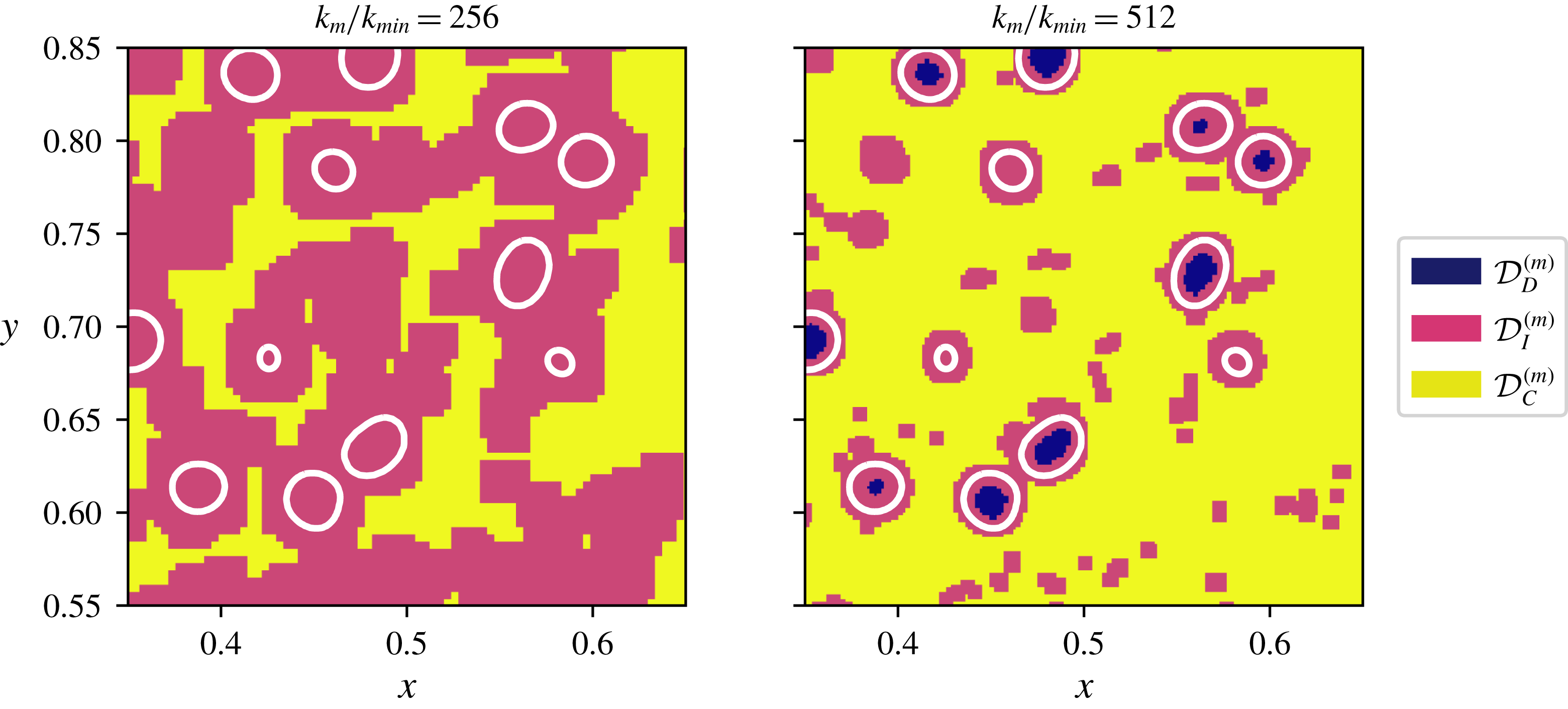
Example of decomposition
 ${\mathcal{D}}^{(m)}={\mathcal{D}}_{C}^{(m)}\cup {\mathcal{D}}_{D}^{(m)}\cup {\mathcal{D}}_{I}^{(m)}$
for case C with
 $k_{m}/k_{min}=256$
and
 $512$
(
 $m=2$
and
 $1$
) in a subregion of the
 $x$
–
 $y$
plane for
 $z=0.5$
.

Then, according to these definitions,
 $\widetilde{E}$
is decomposed as
 $$\begin{eqnarray}\displaystyle \widetilde{E}(k_{m})={\displaystyle \frac{|{\mathcal{D}}_{C}^{(m)}|\widetilde{E}_{C}(k_{m})+|{\mathcal{D}}_{D}^{(m)}|\widetilde{E}_{D}(k_{m})+|{\mathcal{D}}_{I}^{(m)}|\widetilde{E}_{I}(k_{m})}{|{\mathcal{D}}^{(m)}|}}, & & \displaystyle\end{eqnarray}$$
where
 $|\cdot |$
denotes the number of points in the set and, omitting the dependence on
 $k_{m}$
,
 $$\begin{eqnarray}\displaystyle \widetilde{E}_{C}=C_{m}\mathop{\sum }_{i=1}^{3}\mathop{\left\langle \frac{1}{2}\mathop{\sum }_{q=1}^{7}w_{i}^{(m,q)}[\boldsymbol{l}]^{2}\right\rangle }\nolimits_{\boldsymbol{l}\in {\mathcal{D}}_{C}^{(m)}},\quad {\displaystyle \frac{\unicode[STIX]{x2202}}{\unicode[STIX]{x2202}t}}\widetilde{E}_{C}=\widetilde{T}_{C}-\widetilde{V}_{C}, & & \displaystyle\end{eqnarray}$$
 $$\begin{eqnarray}\displaystyle \widetilde{E}_{D}=C_{m}\mathop{\sum }_{i=1}^{3}\mathop{\left\langle \frac{1}{2}\mathop{\sum }_{q=1}^{7}w_{i}^{(m,q)}[\boldsymbol{l}]^{2}\right\rangle }\nolimits_{\boldsymbol{l}\in {\mathcal{D}}_{D}^{(m)}},\quad {\displaystyle \frac{\unicode[STIX]{x2202}}{\unicode[STIX]{x2202}t}}\widetilde{E}_{D}=\widetilde{T}_{D}-\widetilde{V}_{D}, & & \displaystyle\end{eqnarray}$$
 $$\begin{eqnarray}\displaystyle \widetilde{E}_{I}=C_{m}\mathop{\sum }_{i=1}^{3}\mathop{\left\langle \frac{1}{2}\mathop{\sum }_{q=1}^{7}w_{i}^{(m,q)}[\boldsymbol{l}]^{2}\right\rangle }\nolimits_{\boldsymbol{l}\in {\mathcal{D}}_{I}^{(m)}},\quad {\displaystyle \frac{\unicode[STIX]{x2202}}{\unicode[STIX]{x2202}t}}\widetilde{E}_{I}=\widetilde{T}_{I}-\widetilde{V}_{I}+\widetilde{S}. & & \displaystyle\end{eqnarray}$$
Also, we use the same technique to decompose the terms of the evolution equation (2.10), as shown in the equations on the right of (2.15)–(2.17), in which
 $\widetilde{S}_{C}=\widetilde{S}_{D}=0$
and
 $\widetilde{S}=\widetilde{S}_{I}$
because
 $\boldsymbol{f}_{\unicode[STIX]{x1D70E}}=0$
everywhere in the field except at the interface. Thus, the direct effect of the surface-tension force contributes directly only to the evolution of
 $\widetilde{E}_{I}(k_{m})$
.
Figure 4 shows an example of the domain decomposition in a plane for case C with the two highest wavenumbers. Note that, when increasing the wavenumber
 $k_{m}/k_{min}$
from 256 to 512, the details of the flow in the vicinity of the droplet interface are represented in more detail since the size of the wavelet basis function used for the analysis becomes smaller. At the largest wavenumber,
 $k_{m}/k_{min}=512$
(for
 $m=1$
), the sym4 wavelet extends eight points in each spatial direction. Because the carrier part of our decomposition cannot contain points at which the wavelet intersects a droplet,
 ${\mathcal{D}}_{C}^{(1)}$
can only include points farther than
 $8\unicode[STIX]{x0394}x$
from the droplet interfaces. This distance is equivalent to
 $D/4$
or
 $5\unicode[STIX]{x1D702}$
. A wavelet centred at any point closer than that to a droplet will always cross its interface. As the wavenumber halves, the size of the wavelet doubles, so for
 $k_{m}/k_{min}=256$
(for
 $m=2$
),
 ${\mathcal{D}}_{C}^{(2)}$
can only include points farther than
 $D/2$
or
 $10\unicode[STIX]{x1D702}$
from the droplet interfaces. And for
 $k_{m}/k_{min}=128$
(for
 $m=3$
),
 ${\mathcal{D}}_{C}^{(3)}$
can only include points farther than
 $D$
or
 $20\unicode[STIX]{x1D702}$
from the droplets. For the cases studied here, our decomposition cannot represent any wavenumbers smaller than
 $k_{m}/k_{min}=128$
(
 $m=3$
) for
 ${\mathcal{D}}_{C}^{(m)}$
because for
 $m=4$
the wavelets become large enough that they cross the droplet interface.
3 Results


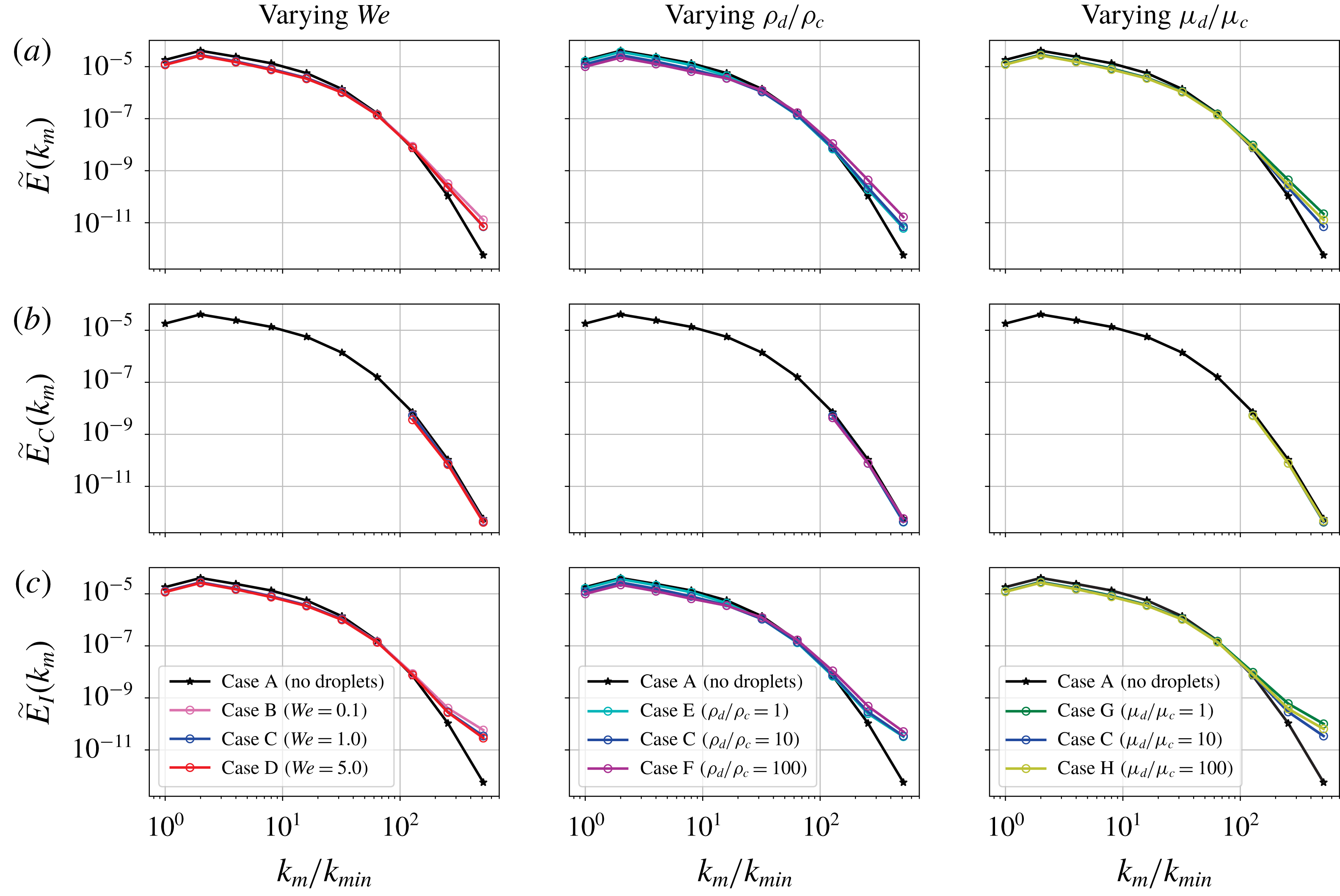
Figure 5 shows the total wavelet spectra
 $\widetilde{E}(k_{m})$
, the carrier wavelet spectra
 $\widetilde{E}_{C}(k_{m})$
and the interaction wavelet spectra
 $\widetilde{E}_{I}(k_{m})$
for all cases A–H. Note that
 $\widetilde{E}_{C}(k_{m})=\widetilde{E}(k_{m})$
for case A and that we plot
 $\widetilde{E}(k_{m})$
of case A for reference in the
 $\widetilde{E}_{I}(k_{m})$
plot. When comparing the spectra of the droplet-laden cases B–H to the droplet-free case A, we notice: (i)
 $\widetilde{E}_{C}(k_{m})$
is nearly unchanged at
 $k_{m}/k_{min}\geqslant 128$
, (ii)
 $\widetilde{E}(k_{m})$
is increased at
 $k_{m}/k_{min}=256$
and
 $512$
and (iii)
 $\widetilde{E}(k_{m})$
is reduced at
 $k_{m}/k_{min}\leqslant 16$
.
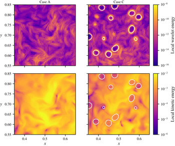
Comparison of local wavelet energy at
 $k_{m}/k_{min}=512$
and local kinetic energy for cases A and C in a subregion of the
 $x$
–
 $y$
plane at
 $z=0.5$
.

(i)
 $\widetilde{E}_{C}(k_{m})$
is nearly the same in all cases for
 $k_{m}/k_{min}\geqslant 128$
. According to (2.15),
 $\widetilde{E}_{C}(k_{m})$
depends on
 ${\mathcal{D}}_{C}^{(m)}$
, which in turn depends on the scale
 $m$
. Because
 ${\mathcal{D}}_{C}^{(m)}$
can only contain points at which wavelets at scale
 $m$
will not extend into any droplets, the closest distance any point in
 ${\mathcal{D}}_{C}^{(m)}$
can be to a droplet is
 $D=20\unicode[STIX]{x1D702}$
,
 $D/2=10\unicode[STIX]{x1D702}$
and
 $D/4=5\unicode[STIX]{x1D702}$
for
 $k_{m}/k_{min}=128$
,
 $256$
and
 $512$
, respectively. Therefore, since
 $\widetilde{E}_{C}(k_{m})$
is nearly the same in all cases, this means that the presence of droplets does not affect the wavelet energy at large wavenumbers
 $k_{m}/k_{min}\geqslant 128$
(i.e. the turbulence scales
 ${\leqslant}5\unicode[STIX]{x1D702}$
) in the flow regions at distances greater than
 $D=20\unicode[STIX]{x1D702}$
from the droplets. For a qualitative display of this phenomenon, figure 6 shows the local wavelet energy at
 $k_{m}/k_{min}=512$
for a subregion of the
 $x$
–
 $y$
plane for the droplet-free case A and droplet-laden case C. The flow regions away from the droplets have nearly the same wavelet-energy magnitude. To explain why the carrier energy at these wavenumbers is unaffected, we analyse the terms of the evolution equation of
 $\widetilde{E}_{C}(k_{m})$
(2.15), namely
 $\widetilde{T}_{C}(k_{m})$
and
 $\widetilde{V}_{C}(k_{m})$
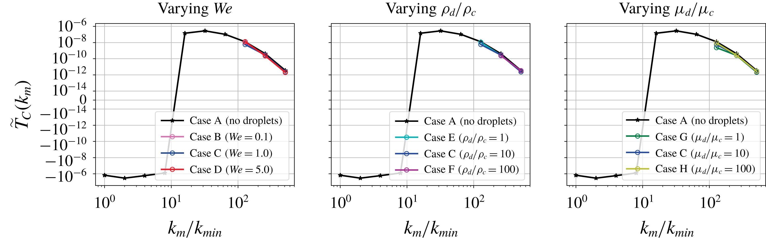
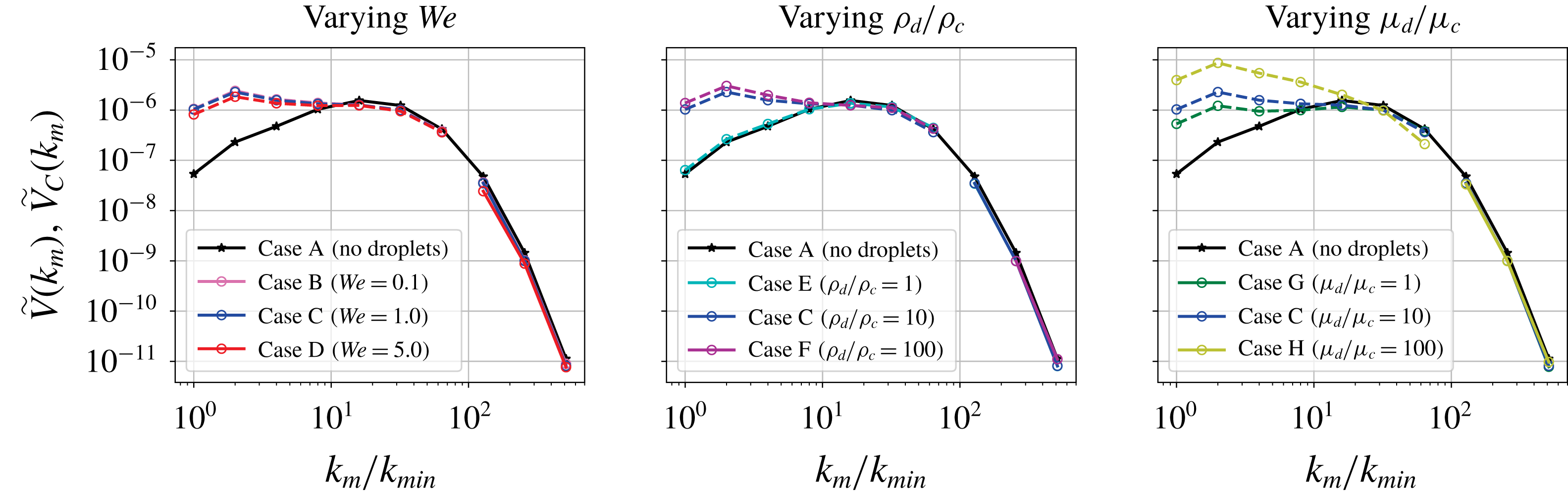
. Figure 8 shows the carrier-phase energy-transfer rate
 $\widetilde{T}_{C}(k_{m})$
, and figure 9 shows the carrier-phase viscous-dissipation rate
 $\widetilde{V}_{C}(k_{m})$
. As for
 $\widetilde{E}_{C}(k_{m})$
,
 $\widetilde{T}_{C}(k_{m})$
and
 $\widetilde{V}_{C}(k_{m})$
are nearly the same in all cases at
 $k_{m}/k_{min}\geqslant 128$
. (Note that, for case F, there is a larger number of smaller droplets due to droplet breakup than in the other cases; consequently,
 ${\mathcal{D}}_{C}^{(m)}$
for
 $k_{m}/k_{min}=128$
has only 164 points and the statistics for this case are thus unreliable and not reported.) Thus,
 $\widetilde{E}_{C}(k_{m})$
evolves nearly at the same rate with and without droplets according to (2.15) because
 $\widetilde{V}_{C}(k_{m})$
and
 $\widetilde{T}_{C}(k_{m})$
are nearly unaffected by the droplets at high wavenumbers. This means that the droplets are not affecting the energy-transfer rate or viscous-dissipation rate at high wavenumbers
 $k_{m}/k_{min}\geqslant 128$
at distances
 ${\geqslant}20\unicode[STIX]{x1D702}$
from their surface, and thus, according to (2.15), they are not affecting the energy
 $\widetilde{E}_{C}(k_{m})$
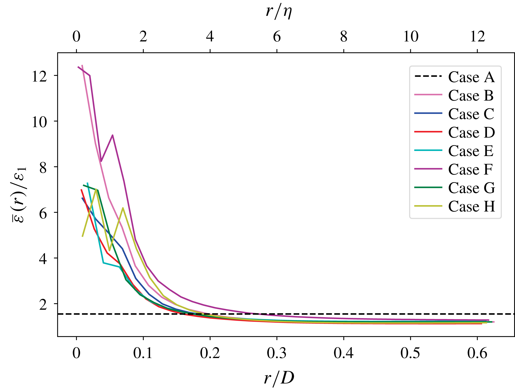
either. To see what is happening in physical space locally as a function of the distance
 $r$
from the droplet interface close to the droplet (for
 $r\leqslant D/4$
), in figure 7, we plot the viscous-dissipation rate
 $\bar{\unicode[STIX]{x1D700}}(r)=2\unicode[STIX]{x1D707}\overline{s_{ij}s_{ij}}/\mathit{Re}$
, where
 $s_{ij}=\frac{1}{2}((\unicode[STIX]{x2202}u_{i}/\unicode[STIX]{x2202}x_{j})+(\unicode[STIX]{x2202}u_{j}/\unicode[STIX]{x2202}x_{i}))$
and the overbar denotes the average over the points at distance
 $r$
from the droplet interface, normalized by the dissipation rate
 $\unicode[STIX]{x1D700}_{1}$
at
 $t=1$
. Droplets increase
 $\bar{\unicode[STIX]{x1D700}}(r)$
near the interface (
 $r\leqslant D/4=5\unicode[STIX]{x1D702}$
) due to the increased velocity gradients near the interface relative to the droplet-free case, and away from the droplet interface (
 $r\geqslant D/4=5\unicode[STIX]{x1D702}$
) the dissipation settles to a uniform value slightly lower than that of single-phase flow due to the overall reduction of TKE. This confirms that away from the droplet interface the region of greatest change here appears to be within approximately
 $D/4=5\unicode[STIX]{x1D702}$
of the droplet (or
 $4\unicode[STIX]{x1D702}$
if we use the Kolmogorov length scale at the time our statistics are computed). Therefore, we conclude that the thickness of the dissipation layer around the droplets is indeed
 $D/4$
as we have seen through our wavelet analysis for the highest wavenumber
 $k_{m}/k_{min}=512$
(besides case F, whose increased density ratio increases the width of the dissipation layer). This result is also confirmed by the physical-space statistics of the topological study of the same data set of Dodd & Jofre (Reference Dodd and Jofre2018).
Viscous-dissipation rate
 $\bar{\unicode[STIX]{x1D700}}(r)$
averaged over points at distance
 $r$
from the nearest droplet interface, normalized by the dissipation rate
 $\unicode[STIX]{x1D700}_{1}$
at
 $t=1$
. The dashed line represents the normalized dissipation rate
 $\unicode[STIX]{x1D700}/\unicode[STIX]{x1D700}_{1}$
at
 $t=3.5$
for the droplet-free case.

(ii)
 $\widetilde{E}(k_{m})$
is higher for the droplet-laden cases than in case A at
 $k_{m}/k_{min}\geqslant 256$
(figure 5
a). According to (2.14),
 $\widetilde{E}(k_{m})$
is a weighted average of
 $\widetilde{E}_{C}(k_{m})$
,
 $\widetilde{E}_{D}(k_{m})$
and
 $\widetilde{E}_{I}(k_{m})$
. The value of
 $\widetilde{E}_{C}(k_{m})$
is nearly the same for all cases (figure 5
b), so it does not contribute to the observed increase at high wavenumbers of
 $\widetilde{E}(k_{m})$
;
 $\widetilde{E}_{D}(k_{m})$
does not contribute much to
 $\widetilde{E}(k_{m})$
because
 ${\mathcal{D}}_{D}^{(m)}$
is always less than
 $2\,\%$
of the domain;
 $\widetilde{E}_{I}(k_{m})$
, instead, is also increased at high wavenumbers by the droplets (figure 5
c). Remember that
 $\widetilde{E}_{I}(k_{m})$
only includes points at which wavelets cross the interface, and the wavelet transform will detect any sharp changes. All of the droplet-laden cases have some degree of velocity non-smoothness at the interface as in figure 2. Decreasing
 $\mathit{We}$
makes the droplets less deformable, increasing
 $\unicode[STIX]{x1D70C}_{d}/\unicode[STIX]{x1D70C}_{c}$
gives the droplets more inertia, and increasing
 $\unicode[STIX]{x1D707}_{d}/\unicode[STIX]{x1D707}_{c}$
increases the difference between
 $\unicode[STIX]{x2202}u_{c}/\unicode[STIX]{x2202}x_{i}$
and
 $\unicode[STIX]{x2202}u_{d}/\unicode[STIX]{x2202}x_{i}$
across the interface (Dodd & Ferrante Reference Dodd and Ferrante2016, § 3.4.4). These factors cause the velocity gradients to peak at the droplet interface and in turn
 $\widetilde{E}_{I}(k_{m})$
to contain more energy at high wavenumbers, and this increase is reflected in
 $\widetilde{E}(k_{m})$
, which is slightly lower than
 $\widetilde{E}_{I}(k_{m})$
due to the averaging with
 $\widetilde{E}_{C}(k_{m})$
. This is the same phenomenon that causes an oscillating increase in energy at high wavenumbers for the Fourier energy spectrum (figure 1). However, thanks to our novel wavelet-spectrum decomposition, we are able to isolate this effect to the portion of the domain containing the interface.
Carrier-phase energy-transfer rate
 $\widetilde{T}_{C}(k_{m})$
(2.11).


(iii)
 $\widetilde{E}(k_{m})$
is lowered for the droplet-laden cases with
 $\unicode[STIX]{x1D70C}_{d}/\unicode[STIX]{x1D70C}_{c}>1$
at
 $k_{m}/k_{min}\leqslant 16$
with respect to that of case A (figure 5
a). This effect can also be seen to a lesser extent in the Fourier energy spectrum in figure 1. The only parameter that changes the amount of this decrease is the density ratio: case F has the highest density ratio and shows the greatest decrease; case E is the only droplet-laden case with density ratio
 $1$
, and it shows nearly no decrease at these wavenumbers. This pattern suggests that energy is decreased at low wavenumbers due to the increased inertia of higher-density droplets. According to (2.10), the evolution of
 $\widetilde{E}(k_{m})$
depends on
 $\widetilde{V}(k_{m})$
,
 $\widetilde{T}(k_{m})$
and
 $\widetilde{S}(k_{m})$
. However, we focus our attention on
 $\widetilde{V}(k_{m})$
because
 $\widetilde{S}(k_{m})$
is one order of magnitude smaller than
 $\widetilde{V}(k_{m})$
and
 $\widetilde{T}(k_{m})$
, while
 $\widetilde{T}(k_{m})$
is not as significantly affected by the droplets as
 $\widetilde{V}(k_{m})$
. Droplets with higher density than the surrounding fluid increase the dissipation rate
 $\widetilde{V}(k_{m})$
at low wavenumbers, as shown in figure 9, by increasing the velocity gradients occurring in the flow. Because of their higher inertia, they will disturb the large-scale eddies more by being more resistant to the carrier flow motion with respect to no droplets (case A) or buoyant droplets (case E). In summary, while droplets with density ratio
 $1$
(case E), by not changing
 $\widetilde{V}(k_{m})$
at low wavenumbers with respect to case A, do not change
 $\widetilde{E}(k_{m})$
at low wavenumbers according to (2.10), droplets with increasing density ratio from
 $10$
to
 $100$
, by increasing the dissipation rate
 $\widetilde{V}(k_{m})$
at the low wavenumbers
 $k_{m}/k_{min}\leqslant 16$
with respect to case A, reduce
 $\widetilde{E}(k_{m})$
at these wavenumbers according to (2.10).
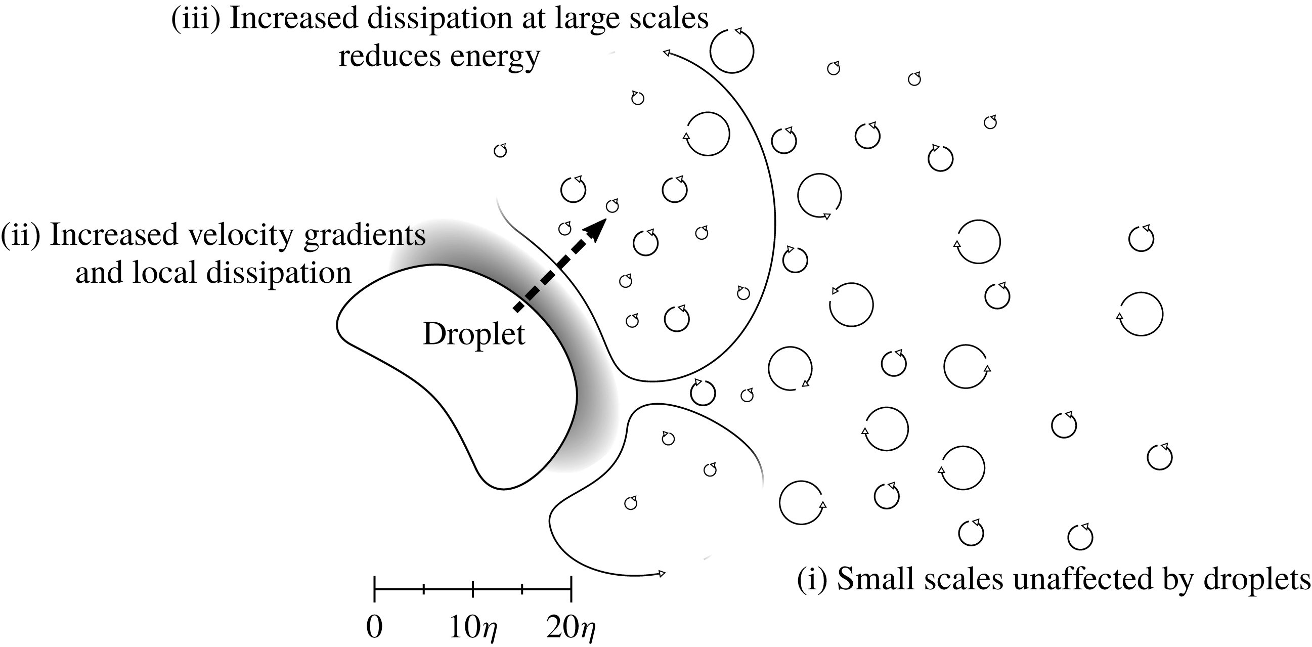
Schematic of results (i)–(iii).

4 Conclusion
We have presented the wavelet energy-spectrum equations, proposed a new decomposition for two-fluid incompressible isotropic turbulence, and applied it to analyse the DNS data set of droplet-laden decaying isotropic turbulence of Dodd & Ferrante (Reference Dodd and Ferrante2016). The proposed domain decomposition allows separating the effects of droplets on the spectra of carrier flow, droplet flow and flow regions crossing the interface. Our results show that, at an average distance from the droplets larger than
 $5\unicode[STIX]{x1D702}$
or
 $D/4$
and at high wavenumbers (
 $k_{m}/k_{min}\geqslant 128$
), the carrier-phase spectra are nearly unaffected by the droplets for the given parameter set (in particular for a volume fraction of
 $5\,\%$
). Also, droplets increase the energy at high wavenumbers (
 $k_{m}/k_{min}\geqslant 256$
) near the interface due to the local larger velocity gradients. Furthermore, the droplets increase the dissipation rate at low wavenumbers (
 $k_{m}/k_{min}\leqslant 16$
) and thereby decrease the TKE spectra at those wavenumbers. A visual summary of these results is given in the schematic of figure 10.
Note that our results do not easily lend themselves to a power-law analysis. For one, the wavelet spectra do not necessarily have the same slopes as their Fourier counterparts (Perrier et al.
Reference Perrier, Philipovitch and Basevant1995). Secondly, our Reynolds number is not high enough (
 $\mathit{Re}_{\unicode[STIX]{x1D706}}=83$
) to see an inertial subrange of wavenumbers (see the dashed lines of figure 1), which is instead present at
 $\mathit{Re}_{\unicode[STIX]{x1D706}}\gtrsim 257$
(see figure 3 of Ishihara, Gotoh & Kaneda (Reference Ishihara, Gotoh and Kaneda2009)).
These results show that wavelets are an important tool for understanding the physics of multiphase turbulence. In particular, this may open new avenues to formulate LES models for multiphase flows. Because we decomposed droplet-laden DNS results and saw that spectral effects of the droplets were restricted to nearby regions at distances from the droplets smaller than
 $D/4$
, especially that
 $\widetilde{V}_{C}(k_{m})$
and
 $\widetilde{E}_{C}(k_{m})$
were unaffected by the droplets at high wavenumbers. This indicates that an LES model in a flow configuration similar to the one described here could still model the subgrid scales at distances larger than
 $D/4$
or
 $5\unicode[STIX]{x1D702}$
from the droplets as single-phase flow. The wavelet decomposition could also have useful applications to related multiphase experiments. For example, the time-series velocity data gained from hot-film anemometry in bubbly flows typically contain velocity spikes due to penetration of the bubbles by the probe, similar to the high velocity gradients at the interfaces of our droplets. The wavelet-decomposition method could be used to generate carrier-phase wavelet energy spectra in the frequency domain.
Acknowledgements
This work was partially supported by the National Science Foundation CAREER Award, grant number ACI-1054591, and facilitated through the use of advanced computational, storage and networking infrastructure provided by the Hyak supercomputer system at the University of Washington, Seattle.