1. Introduction
Internal gravity waves, these being propagating disturbances in density stratified fluids, play a multitude of important environmental roles. In both the ocean and the atmosphere, internal waves excited by a variety of processes such as surface storms (Alford Reference Alford2001) and squall lines (Alexander, Holton & Durran Reference Alexander, Holton and Durran1995), to name but two examples, must subsequently propagate through complex density stratifications that often comprise multiple layers of differing or vanishing stratification. The ability of internal waves to transport energy in the ocean (Simmons & Alford Reference Simmons and Alford2012) and momentum in the atmosphere (Alexander, Richter & Sutherland Reference Alexander, Richter and Sutherland2006) under such circumstances has a substantial impact on large-scale circulation patterns.
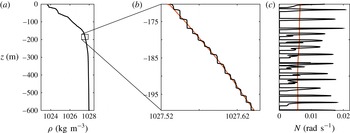
An evolving scenario of interest is the increasingly influential role that internal waves may play in the dynamics of the Arctic Ocean (Rainville, Lee & Woodgate Reference Rainville, Lee and Woodgate2011). Historically, the existence of protective ice cover has shielded the Arctic Ocean from atmospheric storms, and as a result internal wave energy levels in the region have been much weaker than in lower-latitude oceans (Levine, Paulson & Morison Reference Levine, Paulson and Morison1987). The rapid loss of protective ice cover during the summer months, however, suggests that change may be afoot. Moreover, in considering the associated evolution of internal wave activity, a striking feature of the region that must be accounted for is the existence of complex stratifications, such as multiple pycnoclines and intricate double-diffusive staircase structures (Padman & Dillon Reference Padman and Dillon1988), these being a vertical series of mixed layers (i.e. effectively zero stratification) separated by thin stratified layers; an example is presented in figure 1. Such layers are known to extend horizontally for hundreds of kilometres (Timmermans et al. Reference Timmermans, Toole, Krishfield and Winsor2008).
(a) A density stratification profile collected from the Canada Basin in the Arctic Ocean (Rainville & Winsor Reference Rainville and Winsor2008). (b) Magnified view of a section of the profile in (a), revealing the double-diffusive layering structure; the red line indicates a 5 m bin-averaged smoothed density profile. (c) The corresponding buoyancy frequency profiles
 $N(z)$
.

The study of internal wave transmission through mixed layers was initiated by Sutherland & Yewchuk (Reference Sutherland and Yewchuk2004), who used a single mixed layer model and performed complementary experiments; an analogy with quantum mechanical tunnelling was identified. This approach was subsequently extended by Nault & Sutherland (Reference Nault and Sutherland2007) to account for continuously non-uniform density stratifications and vertical shear profiles. Mathur & Peacock (Reference Mathur and Peacock2009) further advanced the methodology to account for internal wave beams, and Mathur & Peacock (Reference Mathur and Peacock2010) demonstrated a direct analogy with the optical transmission properties of a Fabry–Perot interferometer.
The objective of this paper is to consider the propagation of internal waves through stratifications with multiple layers. We start in § 2 by outlining our analytical approach, accounting for viscosity so as to enable comparison with laboratory experiments. In § 3 we use a simple model to demonstrate that the presence of multiple layers has a non-trivial impact. To validate both the model and this fundamental insight, we perform a comparison between theory and laboratory experiments in § 4. Thereafter, we apply our model to an Arctic Ocean stratification and assess the impact of a double-diffusive staircase in § 5. Concluding remarks and future directions are discussed in § 6.
2. Mathematical formulation
To begin, and with a view towards comparisons with laboratory experiments, we consider linear two-dimensional internal waves propagating through a non-uniform background density stratification, satisfying the equation (Sutherland Reference Sutherland2010)
 $$\begin{eqnarray}\partial _{tt}{\rm\nabla}^{2}{\it\psi}+N(z)^{2}\partial _{xx}{\it\psi}={\it\nu}\partial _{t}{\rm\nabla}^{4}{\it\psi},\end{eqnarray}$$
where
 ${\it\psi}$
is the streamfunction,
 $N(z)=\sqrt{(-g/{\it\rho}_{0})\,\text{d}\bar{{\it\rho}}/\text{d}z}$
is the local buoyancy frequency,
 $\bar{{\it\rho}}$
is the background density profile,
 ${\it\rho}_{0}$
is a characteristic density value,
 $g$
is gravity and
 ${\it\nu}$
is the kinematic viscosity. The assumption of harmonic horizontally periodic solutions of the form
 ${\it\psi}\propto {\it\Psi}(z)\exp \text{i}(kx-{\it\omega}t)$
yields the equation
 $$\begin{eqnarray}{\it\Psi}_{zzzz}+\left(\frac{\text{i}{\it\omega}}{{\it\nu}}-2k^{2}\right){\it\Psi}_{zz}+k^{2}\left(k^{2}+\frac{\text{i}{\it\omega}}{{\it\nu}}\left(\frac{N(z)^{2}}{{\it\omega}^{2}}-1\right)\right){\it\Psi}=0.\end{eqnarray}$$
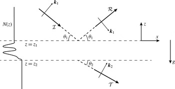
Sketch of the model system. A harmonic plane internal wave of amplitude
 ${\mathcal{I}}$
and wavenumber
 $\boldsymbol{k}_{1}=(k,|m_{1}|)$
incident at angle
 ${\it\theta}_{1}=\tan ^{-1}(k/|m_{1}|)$
to the horizontal, encountering a transition region with multiple layers between
 $z=z_{1}$
and
 $z=z_{2}$
, and emerging with a transmitted amplitude
 ${\mathcal{T}}$
at angle
 ${\it\theta}_{2}=\tan ^{-1}(k/|m_{2}|)$
.

We consider the system presented in figure 2, in which a layered transition region lies between two regions of constant stratification. Within the upper and lower constant-stratification regions the wave field has solutions of the form
 ${\it\Psi}\propto \exp ({\mathcal{M}}z)$
, which upon substitution into (2.2) yields
 $$\begin{eqnarray}{\mathcal{M}}=\pm ({A^{\mp }}^{2}+{B^{\pm }}^{2})^{1/4}\exp (\text{i}\tan ^{-1}(B^{\pm }/A^{\mp })/2),\end{eqnarray}$$
where
 $$\begin{eqnarray}\displaystyle & A^{\mp }=k^{2}\mp \displaystyle \frac{{\it\omega}}{2{\it\nu}}(1+{\it\gamma}^{2})^{1/4}\sin (\tan ^{-1}({\it\gamma})/2), & \displaystyle\end{eqnarray}$$
 $$\begin{eqnarray}\displaystyle & B^{\pm }=\displaystyle -\frac{{\it\omega}}{2{\it\nu}}\pm \frac{{\it\omega}}{2{\it\nu}}(1+{\it\gamma}^{2})^{1/4}\cos (\tan ^{-1}({\it\gamma})/2) & \displaystyle\end{eqnarray}$$
 $$\begin{eqnarray}{\it\gamma}=4{\it\nu}k^{2}N^{2}/{\it\omega}^{3}.\end{eqnarray}$$
Of the four eigenvalue solutions, two correspond to weakly damped internal waves and two correspond to highly damped oscillatory boundary layers. We neglect the boundary layer solutions, and retain only the weakly damped solutions,
 ${\mathcal{M}}(A^{-},B^{+})$
, for which
 $k\ll \sqrt{{\it\omega}/{\it\nu}}$
. As a result, the vertical wavenumber has the expected inviscid component:
 $$\begin{eqnarray}m_{i}\equiv \text{i}\;\text{Im}({\mathcal{M}}_{i}(A^{-},B^{+}))=\pm k\left(1-\frac{N_{i}^{2}}{{\it\omega}^{2}}\right)^{1/2},\end{eqnarray}$$
where the subscript
 $i=1,2$
indicates the upper and lower constant-stratification regions, and viscous decay is captured by
 $m_{i}^{{\it\nu}}=\text{Re}({\mathcal{M}}_{i}(A^{-},B^{+}))$
. It should be noted that by making the complex number
 $i$
explicit in (2.7) our presentation is somewhat different from the traditional presentation, but this has the benefit that for propagating disturbances (i.e.
 $0<{\it\omega}<N_{i}$
), positive (negative) values for
 $m_{i}$
and
 $m_{i}^{{\it\nu}}$
denote downward (upward) energy propagation and decay respectively. For systems in which a constant stratification is never truly achieved, the assumption of plane waves in any given region more formally requires the following Wentzel–Kramers–Brillouin–Jeffreys (WKBJ) condition to be satisfied:
 $$\begin{eqnarray}|m|\gg \left(\frac{k^{2}NN^{\prime }}{{\it\omega}^{2}}\right)^{1/3}.\end{eqnarray}$$
We seek to compute internal wave transmission through a non-uniform stratification
 $N(z)$
with upper and lower boundaries at
 $z=z_{1}$
and
 $z_{2}$
respectively, containing multiple layers in between. To do so, we impose a downward propagating wave at
 $z_{1}$
and solve for the transmitted wave amplitude at
 $z_{2}$
. The general solutions at these two boundaries are written as
 $$\begin{eqnarray}{\it\Psi}=\left\{\begin{array}{@{}ll@{}}\displaystyle {\mathcal{I}}\exp [(m_{1}+m_{1}^{{\it\nu}})z]+{\mathcal{R}}\exp [-(m_{1}+m_{1}^{{\it\nu}})z],\quad & z=z_{1},\\ \displaystyle {\mathcal{T}}\exp [(m_{2}+m_{2}^{{\it\nu}})z],\quad & z=z_{2},\end{array}\right.\end{eqnarray}$$
where
 ${\mathcal{I}}$
is a prescribed incident wave amplitude, and
 ${\mathcal{R}}$
and
 ${\mathcal{T}}$
are respectively the reflected and transmitted wave amplitudes. The boundary conditions in (2.9) can be applied at vertical locations at which (2.8) is satisfied, and there is no requirement that the wave field be WKBJ compliant in between these two boundaries. In order to evaluate (2.2) as a boundary value problem, we write the unknown coefficients
 ${\mathcal{R}}$
and
 ${\mathcal{T}}$
as functions of
 ${\it\Psi}$
so that two conditions are applied at each boundary, namely
 ${\it\Psi}_{z}$
and
 ${\it\Psi}_{zz}$
. The subsequent set of equations are numerically solved using the MATLAB bvp4c function to obtain
 ${\mathcal{R}}$
and
 ${\mathcal{T}}$
.
Having obtained a solution
 ${\it\Psi}(z)$
, this can be used to determine the values of key field variables via standard linear relations. For example,
 $$\begin{eqnarray}\left\{\begin{array}{@{}c@{}}u\\ w\end{array}\right\}=\left\{\begin{array}{@{}c@{}}-{\it\Psi}_{z}\\ \text{i}k{\it\Psi}\end{array}\right\}\exp [\text{i}(kx-{\it\omega}t)],\end{eqnarray}$$
where
 $(u,w)$
is the velocity field.
3. Impact of layering
In the inviscid sharp-interface limit one can derive analytical expressions for
 ${\mathcal{T}}$
and
 ${\mathcal{R}}$
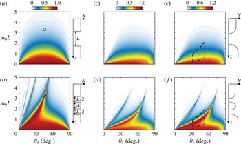
(Sutherland & Yewchuk Reference Sutherland and Yewchuk2004). To demonstrate the non-trivial impact of multiple layers, we briefly consider two straightforward scenarios, illustrated in figure 3: a single mixed layer of depth
 $L$
(identical to Sutherland & Yewchuk (Reference Sutherland and Yewchuk2004)) and a pair of mixed layers of depth
 $L/2$
separated by a stratified layer of width
 ${\it\Delta}=L/2$
. The two systems have the same vertical extent lacking stratification, in which waves are evanescent, but the second system has the additional feature of an intervening stratified layer.
Normalized transmission coefficients for
 ${\it\Psi}$
for sharp-interface systems comprising (a) a single mixed layer of thickness
 $L$
and (b) two mixed layers of thickness
 $L/2$
separated by a stratification layer of thickness
 ${\it\Delta}=L/2$
. The black circle in (a,b) corresponds to
 $m_{0}L\sim 3.5$
and
 ${\it\theta}_{1}=45^{\circ }$
. Panels (c,d) present the corresponding theoretical results for the experimental profiles considered in § 4, incorporating viscosity; panels (e,f) present the corresponding theoretical transmission for total velocity
 $|\boldsymbol{u}|=\sqrt{|u|^{2}+|w|^{2}}$
. The sketches to the right of plots (a,b) and (c–f) illustrate the corresponding stratifications. The dashed regions in plots (e,f) denote the experimental parameter space studied in § 4.

In figure 3(a,b) we present the transmission coefficient (
 $|{\mathcal{T}}|/|{\mathcal{I}}|$
) for the two scenarios as functions of the incident propagation angle
 ${\it\theta}_{1}=\tan ^{-1}(k/|m_{1}|)$
and the evanescent decay exponent
 $m_{0}L$
, where
 $m_{0}=\pm k$
is the evanescent decay scale calculated using (2.7) with
 $N=0$
. As shown in figure 3(a), an internal wave experiences strong transmission for mixed layers that are small compared with the evanescent decay length (i.e.
 $m_{0}L\ll 1$
). Because of interference patterns within the mixed layer, however, there is a clear enhancement in tunnelling for internal waves incident at approximately
 $45^{\circ }$
. The splitting of the mixed layer into two equal parts by a stratified layer adds significant new features, as shown in figure 3(b). There is an intricate sequence of transmission ridges, corresponding to transmission for much larger values of
 $m_{0}L$
than for the single-layer case. For example, the scenario
 $m_{0}L\sim 3.5$
and
 ${\it\theta}_{1}=45^{\circ }$
, for which the single-layer case has effectively zero transmission, has almost complete transmission for the two-layer system.
Varying the value of
 ${\it\Delta}$
alters the specific details of the results, but the qualitative appearance of a sequence of transmission ridges is persistent, and in the limit of
 ${\it\Delta}\rightarrow 0$
the results in figure 3(b) collapse to those in figure 3(a). Extending the study to a stratification comprising three layers and/or layers of greater or lesser strength than the upper and lower bounding stratifications produces qualitatively similar results, with transmission ridges. The existence of these transmission ridges can be attributed to the interplay between the interference patterns of evanescent waves in the mixed layers (Sutherland & Yewchuk Reference Sutherland and Yewchuk2004) and propagating waves within the stratified layers (Ghaemsaidi Reference Ghaemsaidi2015).
There is huge scope for variation of parameters, as one could also consider the impact of mixed layers and intermediate stratification layers of varying thickness, of varying intermediate stratification, and of having any number of layers; it would be easy to become overwhelmed. As such, there is one key message to take away from this motivating example: the impact that multiple layering has on the transmission properties of a stratification can be complex and depend sensitively on the details of the layering structure.
4. Experimental studies
4.1. Apparatus & methods
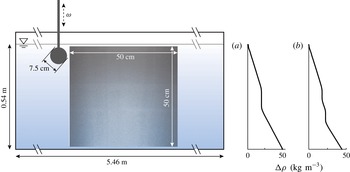
As illustrated in figure 4, experiments were performed in 0.54 m deep salt-stratified water housed in a glass wave tank 5.46 m long and 0.55 m wide. A partition running along the length of the tank created a working section of width 0.2 m, and parabolic reflection barriers positioned at both ends of the tank reflected waves generated in the working section to the rear 0.35 m wide dissipation section (Echeverri Reference Echeverri2009). Filling of the wave tank was via the traditional double-bucket method and two different stratifications were investigated: a single mixed layer spanning
 ${\sim}7~\text{cm}$
and two mixed layers each of depth
 ${\sim}3.5~\text{cm}$
separated by an
 ${\sim}7~\text{cm}$
deep stratified layer. To create the mixed layers we temporarily paused the double-bucket filling in order to introduce constant-density fluid into the wave tank. The density stratifications were measured using a calibrated Precision Measurements Engineering probe attached to a Parker linear traverse for position control; the buoyancy frequency and density profiles are shown in figures 3(e,f) and 4(a,b) respectively.
Schematic of the experimental arrangement and the two measured density stratifications,
 ${\rm\Delta}{\it\rho}={\it\rho}-1000$
, for (a) the single- and (b) the double-mixed-layer studies. A cylinder, positioned 2 cm below the free surface, was used to generate a downward left to right propagating internal wave beam that was visualized by means of particle image velocimetry (PIV); an actual raw PIV image is overlaid to show the location and size of the field of view.

To create an internal wave field with a dominant characteristic wavenumber, a cylinder of diameter 7.5 cm that spanned the 0.2 m width of the working section of the tank was used to generate a downward propagating internal wave beam of characteristic wavenumber
 ${\sim}45~\text{m}^{-1}$
. The cylinder was oscillated vertically with an amplitude of
 $A=7+0.07~\text{mm}$
over a range of excitation frequencies using a stepper-motor-operated Parker linear traverse. Each excitation frequency was separated by a sufficient amount of time to allow the background stratification to return to its base state, which was persistent throughout the experiment. The frequency range was limited since both the incident and transmitted waves needed to be contained within the
 ${\sim}50\times 50~\text{cm}^{2}$
experimental field of view; lower-frequency wave beams with relatively shallow propagation angles would have required larger fields of view, while higher-frequency wave beams were too steep to reliably differentiate between the incident and reflected wave components. As a result of the parabolic end walls, no unwanted reflections from the tank boundaries were observed.
Hollow glass spheres of
 $8{-}12~{\rm\mu}\text{m}$
diameter and 0.1–1.5 specific gravity were used to seed the stratified fluid. A light sheet created by a pulsed Nd:YAG laser illuminated the particles in the midplane of the working section parallel to the front wall of the tank. An Imager Pro X 4M LaVision CCD camera with a resolution of
 $2042\times 2042$
pixels, positioned 1.2 m in front of the tank, was used to visualize the particles at a frame rate of 16 images per forcing period. The images were calibrated and cross-correlated using the DaVis PIV software package to obtain velocity field data. Since no obvious nonlinear features were observed, the velocity fields were Fourier filtered at the forcing frequency in order to suppress noise.
For comparison with theory, incident across-beam profiles were collected as close to the generation source as possible, and the Fourier spectrum was calculated via
 $$\begin{eqnarray}{\hat{w}}(k)=\int _{-\infty }^{\infty }w({\it\eta})\exp \left(\frac{-\text{i}k{\it\eta}}{\sin {\it\theta}}\right)\,\text{d}{\it\eta},\end{eqnarray}$$
where
 ${\it\eta}=x\sin {\it\theta}+z\cos {\it\theta}$
is the across-beam coordinate. This provided the input data needed for our theoretical model to predict the transmitted and reflected wave fields. For convenience, we make use of another form of the internal wave dispersion relation presented in (2.7),
 ${\it\omega}/N=\sin {\it\theta}$
, where
 ${\it\theta}$
is the angle between the group velocity vector and the horizontal. In order to truncate the integral limits in (4.1), we confirmed that the across-beam profile of the incident wave beam was reasonably contained within the field of view. With
 ${\hat{w}}(k)$
in hand, we computed the vertical structure of the wave field,
 ${\hat{w}}(z;k)$
, for each value of
 $k$
, and constructed the final solution using linear superposition (Mathur & Peacock Reference Mathur and Peacock2009):
 $$\begin{eqnarray}w(x,z,t)=\text{Re}\left\{\int _{0}^{\infty }{\hat{w}}(z;k)\exp (\text{i}kx-\text{i}{\it\omega}t)\,\text{d}k\right\}.\end{eqnarray}$$
For these experiments
 ${\it\nu}=1\times 10^{-6}~\text{m}^{2}~\text{s}^{-1}$
.
4.2. Results
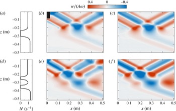
Figures 5(a) and 5(d) present the experimental stratification profiles whose transmission properties are presented as a function of
 ${\it\theta}_{1}$
and
 $m_{0}L$
in figures 3(c,e) and 3(d,f) respectively. The stratification for the first set of experiments comprised a single mixed layer of thickness
 $7.5\pm 0.1~\text{cm}$
(figure 5
a). We note that the lower stratification (
 $N_{2}=1.24~\text{rad}~\text{s}^{-1}$
) is slightly stronger than the upper stratification (
 $N_{1}=0.95~\text{rad}~\text{s}^{-1}$
), and this is readily accounted for in our model. In the second set of experiments, the upper and lower stratifications were the same as in figure 5(a), and the transition region comprised upper and lower mixed layers of thickness
 $3.1\pm 0.1~\text{cm}$
and
 $3.6\pm 0.1~\text{cm}$
, separated by a
 $7.3\pm 0.1~\text{cm}$
stratified layer. Notably, our calculations for the experimental stratifications (figure 3
c–f) retain the key features of the idealized results (figure 3
a,b).
The comparisons of the experimental and theoretical vertical velocity fields in figure 5 show very good agreement; indeed, the differences are almost indiscernible. For the single-layer experiment (figure 5
a–c), we observe an incident wave beam largely reflecting from the mixed layer; a coherent transmitted wave beam is observed below the mixed layer, albeit with a greatly diminished amplitude. For the experiment with two mixed layers, although the total vertical extent of the evanescent behaviour (
 ${\sim}6.7~\text{cm}$
) matches that of the individual-mixed-layer experiment within 10 %, we see a notable increase in the amplitude of the transmitted wave beam (figure 5
d–f). On comparing the experimental and theoretical wave fields for this scenario, some additional features appear in the upper right-hand corner of the experimental results (figure 5
e) compared with the theoretical results (figure 5
f). These are due to reflections of the experimental wave field by the free surface; a process that, for simplicity, was not incorporated into the model.
Results for (a–c) single and (d–f) double mixed layers; snapshots of the experimental (b,e) and theoretical (c,f) vertical velocity wave fields are presented at an arbitrary phase. The wave fields have been normalized by the characteristic vertical velocity amplitude
 $A{\it\omega}$
.

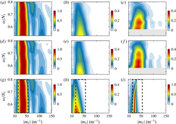
For a more quantitative comparison of the experimental and theoretical results, in figure 6 we present experimental and theoretical Fourier spectra of the total velocity
 $|\boldsymbol{u}|=\sqrt{|u|^{2}+|w|^{2}}$
for the incident and transmitted wave beams as functions of
 $m_{1}$
. Fourier spectra of the transmitted across-beam profiles for single and double mixed layers are shown in figure 6(b,c) for experiments, and the corresponding theoretical predictions are presented in figure 6(e,f). Notably different transmission spectra are observed for the two stratifications, with the transmitted amplitudes in the two-layer case being substantially greater than in the single-layer case.
To connect the experiments to the discussion in § 3, the total velocity transmission spectra presented in figure 3(e,f) are remapped from
 $m_{0}$
to
 $m_{1}$
, and then multiplied by the experimentally measured total velocity incident spectra (figure 6
a) to obtain the theoretical transmission spectra. The results, presented in figure 6(h,i), compare very well with those in figures 6(b,c) and 6(e,f); the two-layer system has stronger transmission and the results for the single-layer stratification similarly show a transmission ridge leaning to the left, in contrast to the rightward-leaning transmission ridge for the double-layer stratification. Notably, the ridge in figure 6(i) is sharper and stronger than those in figure 6(c,f); this is because the experimental field of view was limited in horizontal extent, preventing us from resolving the Fourier transform of the complete transmitted wave field. The results in figure 6(i) nevertheless confirm that the effect we observe is indeed due to a transmission ridge that arises from multiple layering, as delineated by the dashed boundaries in figure 3(e,f), and not due to effects such as the sensitivity of transmission to small changes in the stratification (Gregory & Sutherland Reference Gregory and Sutherland2010).
Experimental total velocity Fourier spectra of the incident wave field (a) and the transmitted wave fields for (b) the single- and (c) the double-mixed-layer stratifications. The total velocity Fourier component has been normalized by the maximum incident value. Panels (d–f) present the corresponding theoretical wave fields. The transmission spectra of the wave fields for a complete field of view are presented in (h) and (i) for the single- and double-mixed-layer stratifications respectively. Panel (a) is reproduced in (d,g), as the experimental incident spectrum is the basis for all three sets of results. The dashed boundary corresponds to that in figure 3(e,f).

5. Geophysical application
We now look to apply the model to study the impact of multiple layering for a geophysical scenario. As an example, we consider the transmission characteristics of the density stratification presented in figure 1, which was collected from the Arctic Ocean during the 2005 Beringia expedition (Rainville & Winsor Reference Rainville and Winsor2008). Given that the geophysical problem is characterized by negligible viscosity and substantial background rotation (at high latitudes), we use the inviscid rotating governing equation:
 $$\begin{eqnarray}{\it\Psi}_{zz}+k^{2}\left(\frac{N(z)^{2}-{\it\omega}^{2}}{{\it\omega}^{2}-f^{2}}\right){\it\Psi}=0,\end{eqnarray}$$
where
 $f$
is the Coriolis parameter. For this formulation, the vertical wavenumber in a constant-
 $N_{i}$
region is
 $$\begin{eqnarray}m_{i}=\pm k\left(\frac{{\it\omega}^{2}-N_{i}^{2}}{{\it\omega}^{2}-f^{2}}\right)^{1/2},\end{eqnarray}$$
and this is substituted into (2.9) (with
 $m_{i}^{{\it\nu}}$
neglected) at vertical positions of the water column satisfying the modified WKBJ condition:
 $$\begin{eqnarray}|m|\gg \left(\frac{k^{2}NN^{\prime }}{{\it\omega}^{2}-f^{2}}\right)^{1/3}.\end{eqnarray}$$
As detailed in § 2, the boundary value problem is numerically solved to yield
 ${\it\Psi}(z)$
, which is then used to obtain other key field variables via standard linear relations. For example,
 $$\begin{eqnarray}\left\{\begin{array}{@{}c@{}}u\\ w\\ {\it\delta}\\ p\end{array}\right\}=\left\{\begin{array}{@{}c@{}}-{\it\Psi}_{z}\\ \text{i}k{\it\Psi}\\ -k{\it\Psi}/{\it\omega}\\ {\it\rho}_{0}(f^{2}-{\it\omega}^{2}){\it\Psi}_{z}/(k{\it\omega})\end{array}\right\}\exp [\text{i}(kx-{\it\omega}t)],\end{eqnarray}$$
where
 ${\it\delta}$
is the isopycnal displacement and
 $p$
is the pressure field.
The continuous density profile shown in figure 1(b) is characterized by thin stratified layers separated by mixed layers produced by double-diffusive instabilities. The corresponding buoyancy frequency profile (figure 1
c) consists of fine peaks of large
 $N$
separated by
 $O(1)$
m layers of
 $N\approx 0$
. For this illustrative example, we assume that the buoyancy frequency is constant above
 $-$
170 m and below
 $-$
200 m, and matches the
 $N$
values at the respective boundaries, thus satisfying (5.3). This staircase stratification differs from the idealized profiles considered in §§ 3 and 4 in that the stratified layers are thinner than the mixed layers and are of notably higher
 $N$
than the mean background stratification. As we shall see, however, the existence of transmission peaks and troughs is again a standout feature of the results.
To assess the impact of double-diffusive layering, we compare the transmission properties of the staircase structure with those of a bin-averaged profile, indicated in figure 1(b,c) by the black and red lines respectively. We compute
 ${\mathcal{T}}({\it\omega};{\it\lambda}_{z})$
as a function of frequency for prescribed vertical wavelengths. Over the Canada Basin, the inertial period ranges from
 $T_{f}=12.15$
to 12.45 h, yielding
 $f\approx 1.42\times 10^{-4}~\text{s}^{-1}$
, which sets the lower bound on wave frequency. Characteristic vertical wavelengths for near-inertial waves in this region are in the range 10–50 m (Cole et al.
Reference Cole, Timmermans, Toole, Krishfield and Thwaites2014). Via the linear relations in (5.4) we calculate the transmission of the time-averaged total energy flux,
 $\boldsymbol{{\mathcal{E}}}=\langle p\boldsymbol{u}\rangle$
.
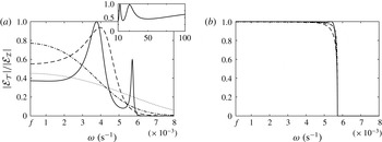
Transmitted energy flux (period averaged in
 $t$
) normalized by the incident energy flux,
 $|{\mathcal{E}}_{{\mathcal{T}}}|/|{\mathcal{E}}_{{\mathcal{I}}}|$
, as a function of excitation frequency
 ${\it\omega}$
, for (a) the staircase and (b) the 5 m bin-averaged stratifications. Incident vertical wave lengths are
 ${\it\lambda}_{z}=10~\text{m}$
(——), 20 m (– – –), 30 m (— ⋅ —) and 50 m (
 $\cdots \cdot$
). The inset shown in (a) presents the near-inertial wave (
 ${\it\omega}=1.05f$
) energy transmission against vertical wavelength
 ${\it\lambda}_{z}$
.

We first consider the staircase stratification profile, for which the results for the energy flux transmission ratio,
 $|{\mathcal{E}}_{{\mathcal{T}}}|/|{\mathcal{E}}_{{\mathcal{I}}}|$
, are presented in figure 7(a). For an incident vertical wavelength of
 ${\it\lambda}_{z}=10~\text{m}$
, we see
 ${\sim}60\,\%$
suppression of energy flux for near-inertial waves (i.e. low-frequency disturbances near
 $f$
). There are two transmission peaks, at
 ${\it\omega}\approx 0.004~\text{s}^{-1}$
and
 ${\it\omega}\approx 0.0055~\text{s}^{-1}$
; for
 ${\it\omega}\gg 0.006~\text{s}^{-1}$
there is no energy flux transmission as the internal waves are evanescent below 200 m. The results are quite similar for internal waves of vertical wavelength 20 m, with
 ${\sim}40\,\%$
suppression of near-inertial wave energy flux, but only a single transmission peak in the midfrequency range. Detuning of the transmission spectra is observed for larger
 ${\it\lambda}_{z}$
, which is characterized by a monotonic decline in transmission between low- and high-frequency waves.
The dynamic regime of the Arctic Ocean system is such that interference prominently impacts near-inertial wave energy transmission, which is a key frequency band. We see clear indications of constructive and destructive interference taking place among the shallow propagating (
 ${\it\omega}=1.05f$
) near-inertial waves over the range
 $10~\text{m}<{\it\lambda}_{z}<50~\text{m}$
, as denoted by the transmission peaks and troughs in the inset of figure 7(a). As
 ${\it\lambda}_{z}$
increases above 100 m, however, the transmission of near-inertial wave energy increases monotonically; in this regime (
 $m_{0}L\ll 1$
) there is very little evanescent decay and effectively complete transmission across a mixed layer, as shown by the model results in figure 3(a). The transmission properties of the bin-averaged stratification (shown in figure 1
c) are presented in figure 7(b). For
 $10~\text{m}<{\it\lambda}_{z}<50~\text{m}$
, all temporal frequencies with
 $f<{\it\omega}<N$
have complete transmission, the energy flux sharply dropping to zero upon transition into the evanescent regime, as expected.
Given the apparent sharpness of the density staircase structure in figure 1(b), and the corresponding spikes in the stratification presented in 1(c), it is interesting to ascertain what role interfacial waves play in determining the transmission and reflection parameters (Sutherland & Yewchuk Reference Sutherland and Yewchuk2004). The significance of interfacial waves compared with the background internal wave field can be quantified by considering the ratio of the wave and hydrostatic pressures acting across a relatively thin stratified layer separating two relatively thick mixed layers. This pressure ratio is (Drazin & Reid Reference Drazin and Reid1981)
 $$\begin{eqnarray}\mathscr{P}=\frac{{\rm\Delta}p}{{\rm\Delta}{\it\rho}g{\it\delta}}=\frac{{\it\omega}\sqrt{{\it\omega}^{2}-f^{2}}}{gk({\rm\Delta}{\it\rho}/{\it\rho}_{0})},\end{eqnarray}$$
where
 ${\rm\Delta}{\it\rho}$
is the density jump between two adjacent mixed layers and
 ${\rm\Delta}p$
is the jump in dynamic pressure associated with the background wave field. For the transmission curves shown in figure 7(a),
 $\mathscr{P}\ll 1$
for
 ${\it\omega}\sim f$
(i.e. the near-inertial regime); as a result, the interference of interfacial waves plays a role in the transmission process for this regime. Another way to consider this is via the dispersion relations for internal and interfacial waves. The internal wave dispersion relation is
 $$\begin{eqnarray}{\it\omega}^{2}=\frac{N^{2}k^{2}+f^{2}m^{2}}{|\boldsymbol{k}|^{2}},\end{eqnarray}$$
and the dispersion relation for an interfacial wave in an unbounded two-layer fluid is
 $$\begin{eqnarray}{\it\omega}^{2}\simeq \frac{gk({\rm\Delta}{\it\rho}/{\it\rho}_{0})}{2}.\end{eqnarray}$$
For the Arctic layering scenario, where
 ${\rm\Delta}{\it\rho}/{\it\rho}_{0}\sim O(10^{-5})$
, one finds that the internal and interfacial wave dispersion curves are in close proximity to each other in the near-inertial regime (i.e.
 ${\it\omega}\sim f$
), revealing that is possible for the passing internal wave field to excite and couple with interfacial waves. For
 ${\it\omega}\sim 10f$
, however, the two dispersion curves diverge from one another and it is no longer possible for the internal wave field to excite interfacial waves.
The details of the transmission spectra presented in figure 7 are sensitive to the particulars of the density stratification; for example, reducing or increasing the flanking
 $N$
values or altering the strength, size, spacing and number of intermediate layers can reduce or increase the transmission to the deep ocean. However, the key message remains unchanged, namely we find two sets of strikingly different results for the actual and smoothed versions of an Arctic Ocean density stratification. The presence of a staircase structure within the water column yields a rich landscape of energy transmission that is dependent on the time and length scale of the incident wave. Smoothing such stratifications, by means of bin averaging, eliminates the distinct features of the Arctic water column and in turn provides an erroneous prediction of energy transmission to the deep ocean.
6. Conclusion
We have performed a fundamental study of the impact of multiple layers on the propagation of internal waves in a density stratification. Starting with a simple stratification, it was demonstrated that multiple layers can have counterintuitive effects due to the interplay between evanescent and propagating waves in neighbouring layers. A set of laboratory experiments was performed and the experimental results were compared with the predictions of a weakly viscous model; the excellent agreement between the two served to validate the model and its interesting predictions. As a demonstration of the broad applicability of the model, which could be used for ocean or atmosphere inspired studies, we investigated a scenario relevant to the Arctic Ocean, finding that the presence of a double-diffusive staircase structure has a non-trivial effect on wave transmission. The degree of wave interference within the multiple layers, which is dependent on the time and length scale of the internal waves, is a prime determinant of transmission, and the relevance of interfacial waves was considered. These results apply to any layered system, and it is not necessary that the origin of the layering be a double-diffusion mechanism. Future research directions of interest would be to ascertain whether the presence of layering can promote or suppress the onset of instability and associated internal-wave-driven mixing, and to incorporate the impact of vertical shear.
Acknowledgements
The authors thank the three anonymous reviewers whose comments notably improved the quality of the paper.