1. Introduction
One of the most important goals of a society is to improve individual quality of life. A common approach to measuring quality of life across locations is to estimate compensating differentials that take into account various factors including income, housing and amenities as revealed through markets (Hoch and Drake, Reference Hoch and Drake1974; Mulligan and Carruthers, Reference Mulligan, Carruthers, Marans and Stimson2011; Powell and Shan, Reference Powell and Shan2012; Hall and Greenman, Reference Hall and Greenman2015). Distinct from the nonmarket valuation literature which focuses on individual amenities of interest (Irwin and Bockstael, Reference Irwin and Bockstael2001; Buck et al., Reference Buck, Auffhammer and Sunding2014), the objective of the quality of life estimates is to recover an overall ranking, aggregating individual compensating differentials. While the existing literature is largely focused on developed countries and relies only on housing and labour market differentials (Roback, Reference Roback1982; Gabriel et al., Reference Gabriel, Mattey and Wascher2003; Colombo et al., Reference Colombo, Michelangeli and Stanca2014; Albouy et al., Reference Albouy, Graf, Kellogg and Wolff2016; Reynolds and Weinstein, Reference Reynolds and Weinstein2021), developing countries present new challenges in applying quality of life differentials as they contain a significant agricultural sector. This paper develops a novel compensating differential model of quality of life rankings that introduces an explicit agricultural sector absent in the existing literature.
We use data from a developing country, Indonesia, to demonstrate the applicability of the model in a rapidly growing country with a significant smallholder agricultural sector. We construct regional quality-of-life indices for rankings based on aggregates of individual labour, housing and agricultural sector differentials at two distinct points in time. Estimating changes in quality of life over time allows us to examine how changes in the quality-of-life rankings are reflected in contemporaneous migration flows, and we find net migration flows into high-ranked areas. These findings suggest that quality of life rankings in a developing country context are useful to help inform policymakers and evaluate the potential for internal migration driven by economic development and public investment.
Originating from Roback (Reference Roback1982), the quality-of-life index is constructed as a sum of nonmarket goods weighted by their implicit prices. The equilibrium model illustrates that the implicit prices for the goods are calculated using housing price and wage differentials estimated using hedonic methods. This framework provides a powerful tool to quantify the overall amenity level for residents and facilitates comparison in terms of quality of life among different places. These rankings yield important information for policymakers, as quality of life differentials and changes in these differentials over time provide insights into expected changes in population and can be used to inform infrastructure and public goods investment.
Using Roback's (Reference Roback1982) model and its variants, many papers have demonstrated the existence of compensating differentials in the United States (Blomquist et al., Reference Blomquist, Berger and Hoehn1988; Beeson and Eberts, Reference Beeson and Eberts1989; Gyourko and Tracy, Reference Gyourko and Tracy1991; Gabriel et al., Reference Gabriel, Mattey and Wascher2003; Albouy et al., Reference Albouy, Graf, Kellogg and Wolff2016; Reynolds and Weinstein, Reference Reynolds and Weinstein2021). The quality of life framework has also been empirically applied in a number of diverse settings, both in developed and transition economies (Gabriel and Rosenthal, Reference Gabriel and Rosenthal2004; Chen and Rosenthal, Reference Chen and Rosenthal2008; Bayer et al., Reference Bayer, Keohane and Timmins2009; Grimes et al., Reference Grimes, Preston, Maré, Badenhorst, Donovan, Cochrane, Cameron and Alimi2021). Focusing on Russia, Berger et al. (Reference Berger, Blomquist and Peter2008) estimate the implicit prices of local amenities based on household data in 39 cities and calculate the quality of life in 953 cities. Colombo et al. (Reference Colombo, Michelangeli and Stanca2014) present hedonic estimates of quality of life in Italian cities. Albouy et al. (Reference Albouy, Graf, Kellogg and Wolff2016) adopt the quality of life framework to reveal American households’ preferences on climate amenities. Reynolds and Weinstein (Reference Reynolds and Weinstein2021) find heterogeneous valuation of quality of life across genders for United States’ cities. Unlike conventional hedonic studies focused on particular amenities, these studies concentrate on the aggregate quality-of-life rankings that illustrate overall amenity levels in equilibrium instead of the identification of individual amenity willingness to pay. While study areas differ, the primary focus of much of the existing quality of life literature is on urban areas, often ignoring the large tracts of rural areas common in many developing countries.
Local economies in developing countries are often dependent on agricultural production in the form of small farms, which may be partly or completely subsistence-oriented (Hazell et al., Reference Hazell, Poulton, Wiggins and Dorward2010). Unlike farm proprietors or hired farmworkers in developed countries, most of the farm labourers in developing countries, including Indonesia, have long cultivated on hereditary or customary land with often overlapping land use claims and ill-defined property rights (Resosudarmo, Reference Resosudarmo2004; Engel et al., Reference Engel, López and Palmer2006; Holden and Otsuka, Reference Holden and Otsuka2014; Holden and Ghebru, Reference Holden and Ghebru2016). Therefore, labour is traditionally the primary input into smallholder subsistence farming at the household level. As areas experience economic growth, this smallholder agricultural sector is also likely to serve as a substantial source of labour for the industrial sector (Lewis, Reference Lewis1954; Gollin, Reference Gollin2014).
In developing countries, internal migration often increases with economic growth and urbanisation as economies undergo structural transformation (e.g., Todaro, Reference Todaro1969; Lucas, Jr, Reference Lucas2004). This migration is most often associated with significant rural-urban migration in countries such as China (Zhao, Reference Zhao1999; Meng and Zhao, Reference Meng and Zhao2018), India (Haberfeld et al., Reference Haberfeld, Menaria, Sahoo and Vyas1999) and Indonesia (Lu, Reference Lu2010). Empirical evidence has shown that rural households move to urban areas for various reasons, such as to obtain higher incomes and better quality of life (Williams and Jobes, Reference Williams and Jobes1990; Du et al., Reference Du, Park and Wang2005). On the other hand, economic incentives, family ties and natural amenities in rural areas may result in farmers’ reluctance to migrate (Zhao, Reference Zhao1999; Deller et al., Reference Deller, Tsai, Marcouiller and English2001). Under these circumstances, understanding the interactions among housing markets, labour markets and smallholder agricultural production can help provide a comprehensive picture of how rural households make residential location decisions.
Given the unique role of agriculture in developing countries, including large numbers of smallholder agricultural labourers, internal migration and population flows from rural to urban areas, estimates of compensating differentials and quality of life provide an important lens through which policymakers can examine changes in well-being across space and time and to target public investment. In this paper, we make three key contributions to the existing literature which extends quality of life models for use in developing country contexts. First, we adapt the quality of life framework by adding a smallholder agricultural sector to the model. We distinguish the farm income differential from the off-farm wage differential, allowing us to test for potential heterogeneity in differentials across sectors. Second, we demonstrate how our model can be used at multiple points in time to generate changes in quality of life that are consistent with observed patterns of internal migration. Finally, our application to Indonesia demonstrates how this approach can provide policy-relevant information in settings where markets are not as well functioning as in the traditional developed country setting (Freeman, Reference Freeman, Rodrik and Rosenzweig2010; Marx et al., Reference Marx, Stoker and Suri2013).
2. Theoretical model and empirical strategy
Roback's (Reference Roback1982) seminal work constructed a general equilibrium model which uses land and labour markets to reveal households’ preferences for amenities. In this model, decision makers choose to live in different locations based on their level of amenities and labour market conditions. In equilibrium, migration ensures that each individual achieves the same level of utility so that no one has an incentive to relocate. At equilibrium, an individual's marginal willingness to pay for an amenity is equal to the partial differential of land rent minus that of wage with respect to an amenity:
 \begin{equation}\frac{{{V_{{s_j}}}}}{{{V_w}}} = {l^c}\frac{{dr}}{{d{{\text{s}}_j}}} - \frac{{dw}}{{d{{\text{s}}_j}}}.\end{equation}
The left-hand side (LHS) is the implicit price — marginal willingness to pay for amenity  ${s_j}$ at location j. On the right-hand side (RHS),
 ${l^c}$ is the residential land consumed, and r and w denote the rent and wage, respectively. The interpretation of this relationship is quite intuitive: local land rents will be high if there is an amenity nearby. For a disamenity, local wages are high to compensate for any negative impacts, otherwise people will leave the location with disamenities and the local wages will rise until equilibrium is achieved. To summarise, households pay higher rents and receive lower wages in order to enjoy nearby amenities. This intuitive relationship provides the foundation for recovery of compensating differentials in the quality of life literature.
To introduce rural agricultural areas into the quality-of-life framework, we consider households’ farm income in addition to off-farm wages, assuming there is no barrier to labour mobility across sectors, in addition to zero migration cost as in the Roback model. Adding an agricultural sector to the original quality-of-life framework presents two primary challenges: (1) how to distinguish smallholder farming from off-farm activities in which both marginal returns with respect to labour should be equal in equilibrium; and (2) once identified, how to combine two different income differentials to measure overall implicit prices for amenities.
We introduce a non-constant returns to scale (non-CRS) farming return function 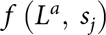 $f\left( {{L^a},{\text{ }}{s_j}} \right)$ as an additional component of the household budget. This function is increasing in labour that is assigned to farming,
 ${L^a}$, and is also affected by amenities
 ${{\text{s}}_j}$ in location j.Footnote 1 This specification assumes that farmers sell products on local markets and directly obtain returns from those, which is common in developing countries that lack large-scale mechanised agricultural industries. In addition, smallholder farming is associated with diminishing returns to scale (DRS) for labour input. This is in contrast to the original quality of life model, where all firms are assumed to be CRS and workers earn fixed wages regardless of labour supply.
The non-CRS assumption fundamentally distinguishes farming returns from wages so that we can obtain amenity contributions to quality of life separately for the agricultural and off-farm labour sectors. In equilibrium, the marginal returns of farming and off-farm activities with respect to labour must be equal. This is because individuals are free to choose to work in either industry or small-scale farming and can move from one sector to another; thus, any difference in the marginal returns from labour between different sectors will be eliminated. In our model, however, the return from farming is not proportional to labour and the partial derivative with respect to amenities does not necessarily equal that of the return from off-farm employment. This provides a key source of variation which is needed for empirical identification of each differential.
3. The utility-maximising problem for households who are small-scale farmers is given by
 \begin{equation}\mathop {\max }\limits_{X,H,{{\text{s}}_j}} u\left( {X,H,{{\text{s}}_j}} \right)\end{equation}
 \begin{align*}s.t.{\text{ }}X + r\left( {{{\text{s}}_j}} \right)H & = w\left( {{{\text{s}}_j}} \right){L^n} + f\left( {{L^a},{\text{ }}{s_j}} \right)\\
& {L^a} + {L^n} = \bar{L}
\end{align*}
where  $X$ denotes a composite commodity consumed and
 $H$ denotes housing.
 $r\left( {{{\text{s}}_j}} \right)$ is the housing price and
 $w\left( {{{\text{s}}_j}} \right)$ is the wage, both of which are functions of local amenities
 ${{\text{s}}_j}$. A household allocates labour to farming,
 ${L^a}$, and off-farm workFootnote 2,
 ${L^n}$, while the total amount of available labour is fixed. Substituting the labour constraint into the budget constraint, we rearrange the first-order conditions to obtain:
 \begin{equation}\frac{{u_{{s_j}}^{\text{*}}}}{{u_X^{\text{*}}}} = {H^{\text{*}}}\frac{{dr}}{{d{{\text{s}}_j}}} - \frac{{dw}}{{d{{\text{s}}_j}}}\left( {\bar L - {L^{a{\text{*}}}}} \right) - \frac{{\partial {f^{\text{*}}}}}{{\partial {{\text{s}}_j}}}\end{equation}
 \begin{equation}w\left( {{{\text{s}}_j}} \right) = \frac{{\partial {f^{\text{*}}}}}{{\partial {L^a}}}.\end{equation}
Consistent with the quality of life literature, income differentials (RHS) are recovered from the implicit prices of amenities (LHS) as high income compensates for lower amenities.Footnote 3 For income differentials, the positive sign of the housing differential illustrates that higher rents offset amenities of higher value. In contrast, the negative sign of the off-farm wage differential suggests that higher wages compensate for the presence of disamenities. This is also true for the farming return differential, though it is distinguished from the wage differential.Footnote 4
After obtaining the three differentials of housing rents, wages and farm returns with respect to an amenity, the implicit price for this amenity can be calculated using equation (3). To obtain the differentials, we estimate the following hedonic regressions:
 \begin{equation}\ln \left( {{r_{ij}}} \right) = {a_0} + a'{A_{ij}} + a''{D_{ij}} + \mathop \sum \limits_k {a_k}{s_{kj}} + {\varepsilon _{ij}}\end{equation}
 \begin{equation}\ln \left( {{w_{ij}}} \right) = {b_0} + b'{B_{ij}} + b''{D_{ij}} + \mathop \sum \limits_k {b_k}{s_{kj}} + {\delta _{ij}}\end{equation}
 \begin{equation}In\left( {{f_{ij}}} \right) = {c_0} + c'{C_{ij}} + c''{D_{ij}} + \sum\limits_k {{c_k}} {s_{kj}} + { \in _{ij}}\end{equation}
where is the kth amenity in location j.  ${a_k}$,
 ${b_k}$ and
 ${c_k}$ are the marginal percentage changes of housing rents, wages and farm income, respectively, with respect to amenity k.
 ${A_{ij}}$,
 ${B_{ij}}$ and
 ${C_{ij}}$ are household or individual characteristics that may lead to idiosyncratic effects on the three prices.
 ${D_{ij}}$ are location controls for economy disequilibrium. Note that in keeping with the quality-of-life literature, we do not aim to estimate causal impacts (Kahn, Reference Kahn1995). Also, we assume that since the unit of analysis is at the individual level i, the level of amenities at a location j is exogenous to the unit of analysis.
To recover compensating differentials, we multiply marginal percentage changes by the mean of rents and incomes. We calculate the quality of life for location  ${\text{ }}j$ by summing all local amenities weighted by their implicit prices. The weighted sum reveals the monetary value of overall amenities in a given location,
 \begin{equation}{Q_j} = \sum_k \left( {{a_k}\bar r - {b_k}\bar w - {c_k}\bar f} \right){s_{kj}}.\end{equation}
4. Data
The primary household-level data used in this paper are obtained from the fourth (in 2007) and fifth (in 2014) waves of the Indonesian Family Life Survey (IFLS) dataset, which tracks the same households over time, forming a panel (Strauss et al., Reference Strauss, Witoelar and Sikoki2016). In 2014, 16,204 households participated in the survey across 13 Indonesian provinces, containing 83 per cent of the total population. In 2007, the survey consisted of 13,535 households. For our analysis, we consider 192 districtsFootnote 5 across 11 provinces on the main islands, including Sumatra, Java, Bali and West Nusa Tenggara (see figure 1).Footnote 6 The survey contains numerous questions about the household, including living conditions, employment and farming business. In the section on housing, each household head reports the annual rents of their residential dwelling or the estimated rents if they own the property. The survey also records a number of housing characteristics based on the head of household's response and the recorder's observation, such as the size and the number of rooms. In the section on employment, respondents report their salaries or net profits from their own business as well as their occupation. Traditional labour characteristics are also reported, including ages, genders, marital status, education, etc. In the section on farm business, household heads report whether or not a family member cultivates a farm land, the net profit, the size of the farm land and the type of crops or livestock. These detailed data enable us to adopt hedonic methods to reveal partial differentials in the three market sectors. All individual characteristics serve as controls to mitigate idiosyncratic effects. See table A1 (online appendix) for a comprehensive list of all the individual controls used in estimation.
Eleven selected provinces in Indonesia.

Apart from individual information, we obtain data on a number of natural and man-made amenities measured at the district level. The district level is the lowest resolution to which the household-level data from the IFLS can be mapped. The variables we calculate at the district level have impacts on quality of life and households’ residential location decisions: the annual average temperature is sourced from the National Oceanic and Atmospheric Administration (Fan and den Dool, Reference Fan and den Dool H2008). The annual precipitation is sourced from Climate Hazards Group InfraRed Precipitation with Station data (Funk et al., Reference Funk, Peterson, Landsfeld, Pedreros, Verdin, Shukla, Husak, Rowland, Harrison, Hoell and Michaelsen2015). Average PM2.5 is sourced from the National Aeronautics and Space Administration (Van Donkelaar et al., Reference Van Donkelaar, Martin, Brauer and Boys2015). We calculate the numbers of volcanic eruptions and floods based on the records in the United Nations disaster information system, DesInventar (United Nations Office for Disaster Risk Reduction, 2017). We calculate the forest area according to the database of Hansen et al. (Reference Hansen, Potapov, Moore, Hancher, Turubanova, Tyukavina, Thau, Stehman, Goetz, Loveland and Kommareddy2013) and the urbanisation rate according to the database of Liu et al. (Reference Liu, Hu, Chen, Li, Xu, Li, Pei and Wang2018). The total population is sourced from Statistics Indonesia, known in Indonesia as BPS (Central Agency on Statistics). Numbers of primary schools, doctors and hospitals per 1,000 population are calculated from the Village Potential Statistics survey conducted by BPS. We proxy healthcare availability using the percentage of immunisation coverage for children under 5 years old and the immunisation rate obtained from the National Socioeconomic Survey conducted by BPS. In addition, we obtain unemployment rates from the BPS Labor Survey to control for disequilibrium. All district-level variables are also presented in table A1.
5. Results
5.1. Hedonic differentials, implicit prices and quality of life
Table 1 shows the results of the housing hedonic regression using the 2014 sample of 11,699 households. All the traditional housing characteristics are significant, with the signs generally consistent with expectations, indicating that the household survey data is of high quality. The key results of interest are the housing rent differentials with respect to amenities in terms of a percentage change. Based on the coefficients, housing rents tend to be low when the weather is very hot and there is excessive rain. Frequent volcanic eruptions are also associated with low housing prices. In contrast, high urbanisation rates make positive contributions to the housing differential. Note that interpretation of these differentials in isolation ignores the important role of labour and agricultural markets on the overall differentiation as the housing market is not the only channel to indicate compensation. The combination of all differentials is needed to obtain a comprehensive picture of the role of amenities in quality of life.
Housing rent equation with amenities, 2014

Notes: Robust standard errors in parentheses (clustered by districts). The regression includes a constant.
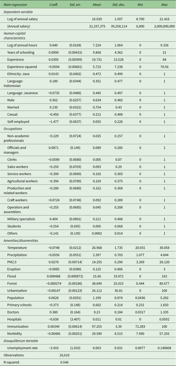
Table 2 presents results for the off-farm labour market using the employment information from 10,610 workers in 2014. These results reveal generally intuitive patterns, such as firms located in districts with severe air pollution are likely to offer higher wages as compensation. Using the data on 2,834 rural households’ information on family farm businesses in 2014, the differentials of smallholder farm income with respect to amenities are shown in table 3 and are noticeably different from those of off-farm wages in table 2. Specifically, excessive rainfall is detrimental to farming returns, which has no significant impact on off-farm wages. However, relative to off-farm labourers (table 2), farmers do not exhibit a strong compensation effect for air pollution (table 3). Urbanisation has a negative impact on farming; however, farmers would rather be close to such an amenity at the expense of lower farm income.
Wage equation with amenities, 2014

Notes: Robust standard errors in parentheses (clustered by districts). The regression includes a constant.
Farm income equation with amenities, 2014

Notes: Robust standard errors in parentheses (clustered by districts). The regression includes a constant.
Using the estimates in tables 1–3, we calculate the overall household-level implicit price in 2014 for each amenity by combining them according to equation (3). In our sample, the average number of workers per household is 2.66. Following Berger et al. (Reference Berger, Blomquist and Peter2008), we multiply the wage differential by this number to obtain the marginal change in household off-farm income. In addition, 31.95 per cent of households in the sample cultivate farmlands. Based on this, we assign household income for the representative household such that 31.95 per cent of the income is from farming and the rest is from off-farm work.Footnote 7 Therefore, we multiply the wage and farm income differentials by 68.05 per cent and 31.95 per cent respectively, in the quality of life formula.
While our primary focus is on the overall quality of life rankings, we nonetheless report the results for the implicit prices for individual amenities in column (4) of table 4. These are the monetary measures for each amenity or disamenity in Indonesian Rupiahs.Footnote 8 Positive prices indicate amenities and negative prices disamenities. For example, air pollution and population are viewed as disamenities while temperature and urbanisation are viewed as amenities up to certain thresholds. Implicit prices indicate the total differential of the effect of an amenity; therefore, significant results provide evidence of the existence of compensating differentials as a whole (Berger et al., Reference Berger, Blomquist and Peter2008).
Implicit prices of amenities, 2014

Notes: Housing rent, and wage and farm income differentials are taken from tables 1, 2 and 3. The annual full implicit prices per household are evaluated at the means of housing rent, wage, and farm income of the sample. 31.95% of households in the sample work for a farm business. For the remaining 68.05% of households, the average number of workers per household is 2.66. 1,000,000 Indonesian Rupiahs are equal to 80.39 US dollars in 2014.
Robust standard errors in parentheses (clustered by districts). The standard errors on the full implicit prices are calculated from a linear combination of the standard errors in the housing rent, wage, and farm income hedonic equations, assuming there is no covariance among the differentials.
We sum the amenities in each geographic district weighted by the full implicit prices.Footnote 9 As a result, we obtain the quality-of-life index for 192 Indonesian districts in 2014. It is not appropriate to directly interpret the monetary index values as quality of life magnitudes due to unit and baseline dependencies across amenities; these index values are typically normalised to be non-negative (see Berger et al., Reference Berger, Blomquist and Peter2008). Therefore, the following analysis focuses on the rankings in 2014, shown in figure 2. It indicates that districts in the east of Java have a relatively higher level of quality of life. In contrast, areas in the west of Java, especially areas around the capital Jakarta, have generally lower quality of life rankings. This result is consistent with well-known congestion and pollution challenges in these rapidly urbanising areas (Yusuf and Resosudarmo, Reference Yusuf and Resosudarmo2009). We illustrate the range of normalised quality-of-life indices by province in figure A1. The spatial pattern of the indices in 2014 is consistent with that of the rankings depicted above.
Choropleth maps illustrating quality-of-life rankings for 192 districts in Indonesia, 2014 and 2007.

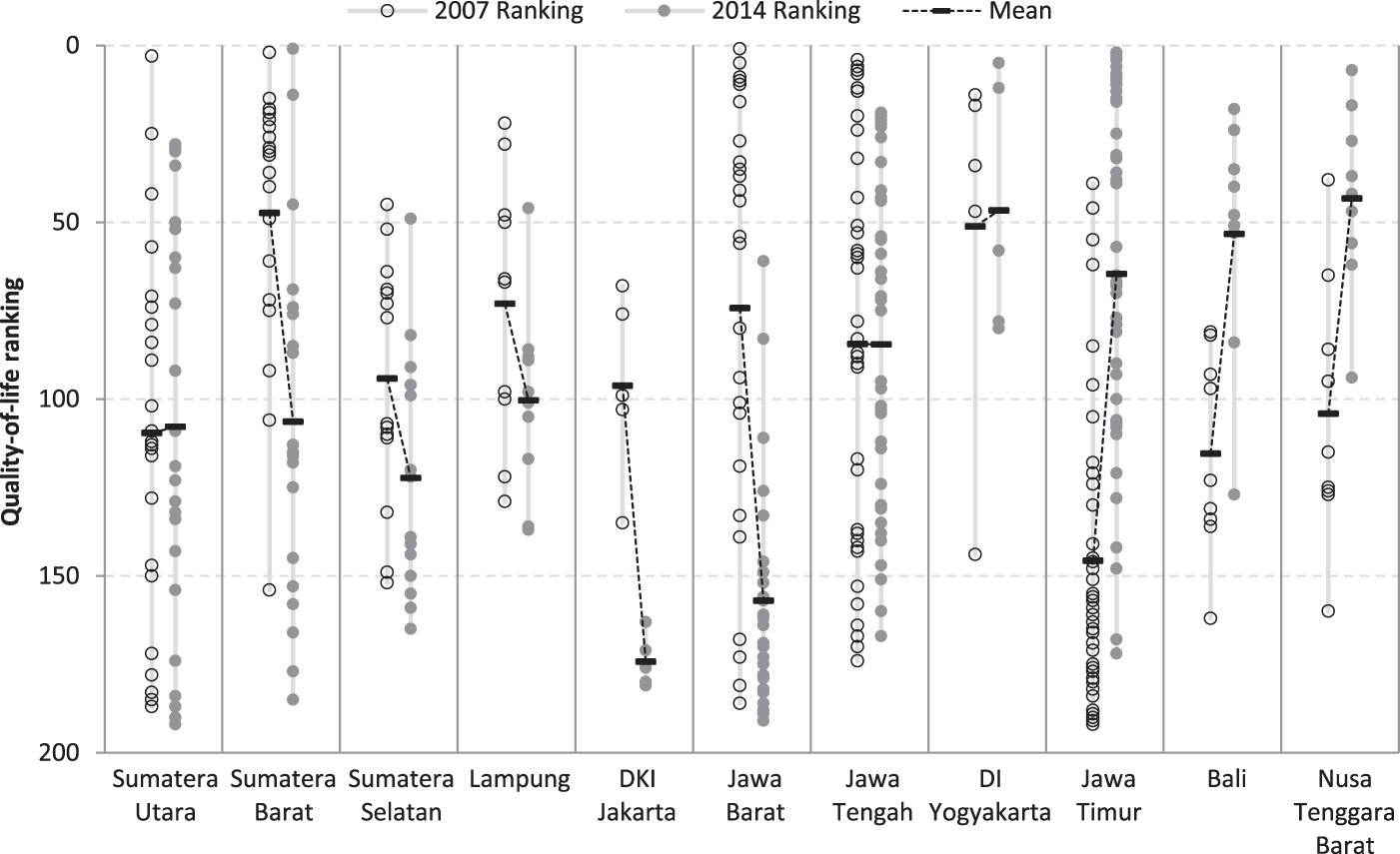
We repeat the same quality of life estimation for each Indonesian district in 2007 (figure 2 and tables A2–A5 in the online appendix). The comparison of the rankings between the two periods is presented in figure 3 and table A6. From 2007 to 2014, the rankings of quality of life changed significantly. At a macro-scale, there is an obvious shift of high-ranking districts from the west of Java to the east (figures 2–3). Districts in the provinces located around the west of Java Island, including DKI Jakarta, Jawa Barat and Lampung, generally experienced decreases in quality-of-life rankings over the sample period. In contrast, districts in the eastern provinces, such as Jawa Timur, Bali and Nusa Tenggara Barat, experienced increases in quality of life rankings.
Quality-of-life rankings for 192 districts in Indonesia, 2007 and 2014.

To compare our preferred model with the conventional quality-of-life model without the agricultural sector, we calculate the quality-of-life indices and rankings only using the housing rent and wage differentials in table A6. Furthermore, we compute the correlation coefficients across ranking methodologies (with vs. without farm income) and across years (2007 vs. 2014) in table A7. Although rankings with and without farm income show high cross-methodological correlations within each year, the between-year correlation becomes statistically insignificant only when farm income is included. This indicates that incorporating the agricultural sector is necessary to detect significant temporal shifts in quality-of-life rankings, particularly the substantial reordering observed over time in agrarian economies undergoing structural transformation, as seen in Indonesia's smallholder-dominated sector.
For robustness, we implement several alternative regression models. First, pooled cross-section regressions with year fixed effects yield implicit prices (table A8) and quality-of-life rankings (table A11) that fall between the 2007 and 2014 baseline estimates (table 4 and tables A5–A6) in magnitude and significance. Second, quantile regressions (25th/50th/75th percentiles) reveal increasing absolute implicit prices for most amenities at higher rent/wage/income percentiles (tables A9–A10), indicating heightened amenity sensitivity among high-expenditure households. Corresponding quality-of-life rankings (table A11) remain consistent with the baseline results. Third, we consider a two-stage hedonic model using estimated district fixed effects as dependent variables, following Albouy et al. (Reference Albouy, Graf, Kellogg and Wolff2016) to address the possible bias caused by omitted amenities and disequilibrium variables. The resulting implicit prices and quality-of-life rankings are highly consistent with the baseline ones (tables A12–A14).
5.2. Changes in quality of life and internal migration
Internal migration in Indonesia is significant and ongoing (Sukamdi and Mujahid, Reference Sukamdi and Mujahid2015). The internal migration patterns are driven by contemporaneous changes in public investment, natural disasters and historical policy interventions.Footnote 10 The transmigration program, initiated by the Dutch colonial government and then taken over by the Indonesian government after independence, aims to relocate residents from densely populated Java to outer islands, in order to relieve demographic pressure and develop unexploited remote lands (Van Lottum and Marks, Reference Van Lottum and Marks2012). In recent years, this program has largely been supplanted by economic incentives, which are now the dominant driver of internal migration (Tirtosudarmo, Reference Tirtosudarmo2009; Van Lottum and Marks, Reference Van Lottum and Marks2012).
Indonesia lacks formal nationwide restrictions on domestic population mobility, allowing residents to move between regions without significant legal barriers. Nevertheless, other non-policy bottlenecks constitute the predominant spatial friction, given Indonesia's geographic characteristics, multiple languages and ethnicities and limited transportation connectivity. For example, the elasticity of migration cost to distance has been calculated as 15 per cent in Indonesia, compared to 2 per cent in the United States (Bryan and Morten, Reference Bryan and Morten2019).
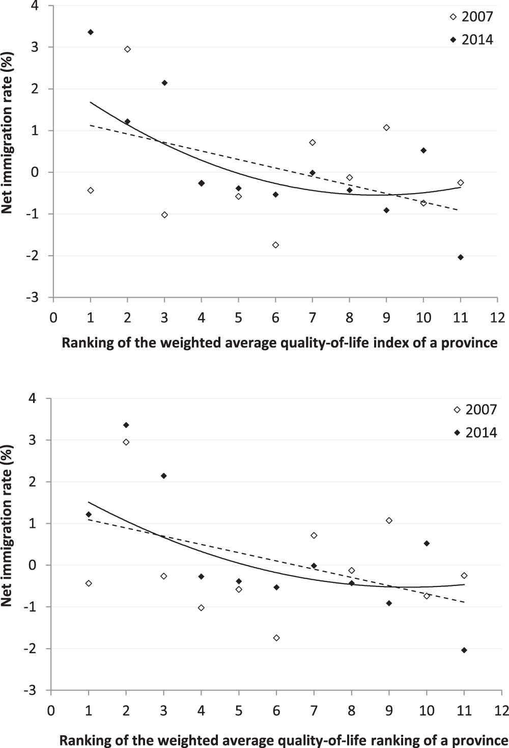
Since our theoretical model is based on households’ residential location choices, we explore the relationship between quality of life and cross-district migration to examine the underlying equilibrium adjustment mechanism. We use scatter plots to present our resulting quality-of-life rankings and the net immigration rates in the corresponding year (sourced from Statistics Indonesia) at the province level (the finest level at which the migration data is available) (figure 4). We calculate the provincial quality-of-life rankings by taking the average of quality-of-life indices of the districts in the province, weighted by district population and then ranking the provinces. We also take the weighted average of individual rankings. In both approaches, the scatter plots show a negative linear relationship, indicating that higher quality of life rankings (smaller numbers) are associated with larger net immigration flows. Moreover, the quadratic fit lines indicate that this relationship is stronger, with steeper slopes, for higher-ranked provinces, i.e., the incremental net migration rate gained from a one-rank increase is greater in provinces with higher quality of life.
Quality-of-life rankings and net immigration rates at the province level, 2007 and 2014.

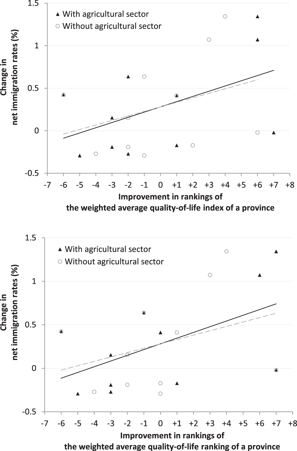
We further consider the improvement in the rankings and the change in net immigration rates from 2007 to 2014 (figure 5). Cancelling out the effects of time invariant unobserved location-specific characteristics, this figure indicates that locations with larger improvements in quality-of-life rankings attract more immigrants, which is consistent with our predictions. The finding demonstrates that Indonesian households’ residential location choices are indeed influenced by quality of life differentials: households tend to move to locations with higher levels of quality of life, leading to a new equilibrium outcome with corresponding shifts in the related markets. As a robustness check, we also replicate the analysis at the district level using the change in district populationFootnote 11 as a proxy for the number of immigrants: the results in figure A2 support our findings.
Improvement in quality-of-life rankings and change in net immigration rates at the province level, 2007-2014.

Finally, to demonstrate the importance of the agricultural sector in our model, we consider the traditional quality-of-life rankings, ignoring the compensating differential from the agricultural sector and show the relationship between rankings and the net immigration rates in terms of changes (figure 5). The upward-sloped linear fit lines for the traditional rankings (grey dashed lines), suggesting a positive relationship between improvement in rankings and change in net immigration rates, are flatter than those for our preferred rankings, including the agricultural sector (black solid lines). This indicates that ignoring the agricultural sector appears to lead to a loss of information in the resulting quality-of-life rankings, and our rankings considering the agricultural sector provide stronger explanatory power for households’ internal migration choices in Indonesia.
6. Discussion
In this paper, we introduce an agricultural sector into the theoretical model of compensating differentials to calculate quality-of-life rankings. By adding a farming return component to the household budget, we can distinguish the farm income differential from the off-farm wage differential. We show that this new framework is well-suited to estimate quality of life in developing country settings with large agricultural sectors, and the changes in quality of life over time are consistent with large internal migration patterns. We find that compensating differentials exist across Indonesia, specifically in the agricultural sector. The farm income compensating differentials differ from the off-farm wage differentials, suggesting that local amenities have heterogeneous impacts on agricultural and off-farm labour markets. Across time, our findings indicate that the rapid development occurring in Indonesia has served to reduce the gap in the quality of life across jurisdictions.
Our quality-of-life rankings from our model are consistent with the expected migration flows of households from lower quality-of-life areas to higher quality-of-life locations. We show that this relationship is significantly stronger when including the agricultural sector in our developing country context. This highlights the importance of accounting for additional dimensions of compensating differentials as economies transition from developing to developed status.
In addition to the overall quality-of-life rankings, the current work also provides a flexible framework for policy-makers to further analyse quality of life in specific aspects. Once the implicit prices are obtained from compensating differentials, one can select relevant amenities to construct indices that reflect local environmental conditions on particular topics of interest. For example, based on estimated implicit prices for amenities that are related to natural resources and disasters, it is possible to construct multiple types of vulnerability indices to focus on topics such as climate change (Barreca, Reference Barreca2012; Zhang et al., Reference Zhang, Zhang and Chen2017). Use of themed indices may also help policymakers assess the effects of specific policies aimed at improving environmental conditions and quality of life, as many related policies have been implemented in Indonesia, such as forest conservation and infrastructure investment (Gibson and Olivia, Reference Gibson and Olivia2010; Koh and Ghazoul, Reference Koh and Ghazoul2010). Our work highlights the importance of considering the agricultural sector as a key input when using quality-of-life indices for policy evaluation.
Supplementary material
The supplementary material for this article can be found at https://doi.org/10.1017/S1355770X25100260.
Acknowledgements
Wei Chen acknowledges financial support from the National Natural Science Foundation of China (No. 72303234).
Competing interests
The authors declare none.