1 Introduction
The ubiquity of internal tides in the ocean has prompted extensive study of their generation at topography, and subsequent radiation (Bell Reference Bell1975; Baines Reference Baines1982; Llewellyn Smith & Young Reference Llewellyn Smith and Young2003). Their role in mixing the stably stratified ocean as they dissipate is well established (Munk & Wunsch Reference Munk and Wunsch1998), and global climate models (GCMs) have provided insight into the remarkable sensitivity of large-scale ocean circulation on the distribution and magnitude of the mixing (Hasumi & Suginohara Reference Hasumi and Suginohara1999; Simmons et al. Reference Simmons, Jayne, St Laurent and Weaver2004; Jayne Reference Jayne2009). As a result, significant effort has been expended developing physically based parameterizations for dissipative processes associated with the superinertial internal tide, i.e. tidal motions with a period of less than one pendulum day (Green & Nycander Reference Green and Nycander2013). These parameterizations are now being implemented in GCMs that are used to inform climate policy (e.g. Melet et al. Reference Melet, Venayagamoorthy, Legg and Polzin2013). In contrast, the mixing associated with subinertial tidal constituents is much less well studied and remains unaccounted for, despite large losses from the subinertial barotropic tide (Egbert & Ray Reference Egbert and Ray2003; Müller Reference Müller2013).
On a traditional
 $f$
-plane, the internal wave dispersion relation disallows radiating internal waves whose period is longer than that of the local pendulum day, which means that subinertial tidal constituents do not generate radiating internal tides polewards of their turning latitudes (defined as where the tidal frequency matches the local Coriolis frequency, and sometimes called a critical latitude). The inclusion of ‘non-traditional’ Coriolis effects extends this latitudinal range by tens to hundreds of kilometres, depending on stratification, enabling subinertial waves to propagate over a limited range (Gerkema & Shrira Reference Gerkema and Shrira2005). However, in regions polewards of this, subinertial tides generate a baroclinic response that is evanescent, decaying exponentially away from topography. Globally these subinertial evanescent tides account for less baroclinic energy than their superinertial radiating counterparts, whose energy forms one of the dominant internal signals in the ocean. Nevertheless, observational and regional modelling studies indicate that the nearfield mixing associated with these trapped tides may be significant (Nakamura et al.
Reference Nakamura, Awaji, Hatayama, Akitomo, Takizawa, Kono, Kawasaki and Fukasawa2000, Reference Nakamura, Isoda, Mitsudera, Takagi and Nagasawa2010; Osafune & Yasuda Reference Osafune and Yasuda2013; Musgrave et al.
Reference Musgrave, Mackinnon, Pinkel, Waterhouse and Nash2016). To understand the role played by tidal dissipation poleward of the turning latitude, it is necessary to have an understanding of both the linear evanescent response and the typical nonlinear responses that arise. In this paper we present an idealized study that explores in detail the nature of the baroclinic response to subinertial tidal forcing at topography, and contrast the physics and processes leading to mixing to those in the relatively well-understood superinertial case.
In the first part of the paper we build on the work of Llewellyn Smith & Young (Reference Llewellyn Smith and Young2003), to derive an analytic solution for subinertial trapped tides generated at a tall, infinitely thin ridge. We show that the baroclinic response is evanescent with a decay scale that decreases with increasing latitude. Both the along-ridge velocity and the near-ridge isopycnal displacement of the evanescent response grow with latitude away from the turning latitude. As a result, for a constant-amplitude barotropic tide, the total near-ridge energy density (i.e. kinetic plus potential) of the subinertial baroclinic response grows with latitude, in direct contrast with the superinertial baroclinic response which has a constant energy density at all latitudes.
We explore and verify these predictions in a series of idealized two-dimensional numerical simulations where a 24 h oscillating tide interacts with a Gaussian ridge at a range of latitudes. Of particular interest is the influence of latitude on the processes leading to turbulence. In the two-dimensional simulations presented here, we use mixing as a proxy for turbulence in the three-dimensional ocean. By performing ‘equivalent’ simulations at superinertial and subinertial latitudes, we find that transient hydraulic jumps are the dominant mechanism for mixing in our simulations when the tide is subinertial, and tidal lee waves formed from radiating constituents are additionally important when the tide is superinertial.
We also investigate the generation of tidally rectified along-ridge currents, whose energy is significant in the nearfield and increases with latitude. These have been examined analytically for both unstratified tidal flows (Huthnance Reference Huthnance1973; Loder Reference Loder1980), and stratified tidal flows over weak topography (Maas & Zimmerman Reference Maas and Zimmerman1989b
; Brink Reference Brink2011). The combination of tall topography and stratification places our simulations beyond the parameter regime of prior theory, but nevertheless we find similar qualitative results of strong along-slope flows, and weaker cross-slope and vertical circulations in the Eulerian time mean. An explicit calculation of particle paths show that particles near the ridge-crest undergo looping trajectories along the flanks for
 $f\neq 0$
.
Observations of enhanced subinertial frequency currents around topography have motivated the investigation of trapped topographic waves (Rhines Reference Rhines1970; Chapman Reference Chapman1989; Brink Reference Brink1990; Padman et al. Reference Padman, Plueddemann, Muench and Pinkel1992; Codiga Reference Codiga1997). These arise from a resonance between the free modes associated with a certain topography and background stratification, and an ambient forcing frequency. The solutions presented in this paper are complementary, describing the forced response to subinertial tides which may be expected even in the absence of a resonance. When the forced response projects onto the free modes of a certain topography, a trapped wave may be resonantly generated.
The remainder of this paper is broadly divided into four parts: the first presents theoretical results for subinertial tidal forcing of a stratified fluid over a knife-edge ridge; the second presents a series of numerical experiments over a tall, narrow Gaussian ridge aimed at verifying the theory, and extending the description to larger amplitude, more nonlinear tides; and the third discusses the relevance of this work to more general three-dimensional situations. In the fourth section we present a summary.
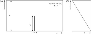
Definition sketch. (a) The barotropic tide oscillates over a tall, narrow ridge. (b) Density,
 ${\it\rho}$
, increases uniformly with depth.

2 Theory
In this section we extend the results of Llewellyn Smith & Young (Reference Llewellyn Smith and Young2003) (hereafter LSY03) to include subinertial tidal forcings. A similar solution for superinertial tides at a knife edge is presented by St Laurent et al. (Reference St Laurent, Stringer, Garrett and Perrault-Joncas2003). The problem is formulated in two dimensions on an
 $f$
-plane, with an imposed barotropic tide (
 $u_{b}=U_{0}\cos {\it\omega}t$
) oscillating in the
 $x$
-direction. The total fluid depth is
 $h$
. At
 $x=0$
the tide interacts with an infinitely thin ridge of height
 $z_{0}$
, where
 $z_{0}<h$
(figure 1). For simplicity we consider only uniform stratification (
 $N$
) in this study, though LSY03 additionally presents solutions for the case of slowly varying
 $N(z)$
. The linearized equations are
 $$\begin{eqnarray}\left.\begin{array}{@{}c@{}}u_{t}-fv=-p_{x},\\ v_{t}+fu=0,\\ p_{z}=b,\\ b_{t}+N^{2}w=0,\\ u_{x}+w_{z}=0,\end{array}\right\}\end{eqnarray}$$
where velocities are
 $(u,v,w)$
, pressure is
 $p$
and the Coriolis frequency is
 $f$
. The density,
 ${\it\rho}$
, has been written in terms of the Brunt–Väisälä frequency,
 $N$
, and the buoyancy,
 $b$
:
 $$\begin{eqnarray}{\it\rho}={\it\rho}_{0}\left[1-\frac{N^{2}z}{g}-\frac{b}{g}\right],\end{eqnarray}$$
and pressure has been scaled by
 ${\it\rho}_{0}$
. Defining a stream function
 $(u,w)=(-{\it\psi}_{z},{\it\psi}_{x})$
, the equations can be combined, and written as
 $$\begin{eqnarray}{\it\psi}_{zztt}+f^{2}{\it\psi}_{zz}+N^{2}{\it\psi}_{xx}=0.\end{eqnarray}$$
Imposing a boundary condition of no-flow through the barrier means
 $$\begin{eqnarray}{\it\psi}(x=0,z<z_{0})=U_{0}z\cos ({\it\omega}t),\end{eqnarray}$$
such that
 $U_{T}=u_{b}+u=U_{0}\cos ({\it\omega}t)+u=0$
on the knife-edge ridge.
In the linear limit we look for solutions which are time periodic at the tidal frequency,
 ${\it\omega}$
:
 $$\begin{eqnarray}\displaystyle {\it\psi}=U_{0}Re\{\text{e}^{-\text{i}{\it\omega}t}{\it\phi}\}. & & \displaystyle\end{eqnarray}$$
Then, equation (2.3) can be written
 $$\begin{eqnarray}N^{2}{\it\phi}_{xx}=({\it\omega}^{2}-f^{2}){\it\phi}_{zz},\end{eqnarray}$$
with boundary conditions
 ${\it\phi}(x=0,z<z_{0})=z$
, and
 ${\it\phi}(x,h)=0$
. For superinertial flows,
 ${\it\omega}^{2}>f^{2}$
and the equation is hyperbolic, however, for subinertial flows,
 ${\it\omega}^{2}<f^{2}$
and the equation is elliptic. The solution is constructed from an infinite sum of the vertical normal modes, defined by
 $$\begin{eqnarray}\frac{\text{d}^{2}a_{n}}{\text{d}z^{2}}+\frac{N^{2}a_{n}}{c_{n}^{2}}=0,\end{eqnarray}$$
with
 $a_{n}(0)=a_{n}(h)=0$
, and
 $\int _{0}^{h}a_{n}(z)a_{m}(z)\,\text{d}z=(h/2){\it\delta}_{mn}$
. A Green’s function solution to (2.6) satisfies
 $$\begin{eqnarray}N^{2}G_{xx}-({\it\omega}^{2}-f^{2})G_{zz}=G_{0}{\it\delta}(x){\it\delta}(z-z^{\prime }),\end{eqnarray}$$
for a point source located at
 $x=0,z=z^{\prime }$
. The normalization
 $G_{0}$
will be determined shortly for convenience. We write the vertical dependence of the separable solution in terms of an infinite sum of vertical normal modes,
 $a_{n}=\sin (nZ)$
,
 $$\begin{eqnarray}G(x,Z,Z^{\prime })=\mathop{\sum }_{n=1}^{\infty }G_{n}(x,Z^{\prime })\sin (nZ),\end{eqnarray}$$
where
 $Z=({\rm\pi}z)/h$
. For modal phase speeds
 $c_{n}=hN/n{\rm\pi}$
, we define two real wave numbers corresponding to the superinertial (
 $\check{~}$
: below the turning latitude) and subinertial (
 $\hat{~}$
: above the turning latitude) cases:
 $$\begin{eqnarray}{\check{k}}_{n}^{2}=\frac{{\it\omega}^{2}-f^{2}}{c_{n}^{2}}\quad \text{and}\quad \hat{k}_{n}^{2}=\frac{f^{2}-{\it\omega}^{2}}{c_{n}^{2}}.\end{eqnarray}$$
The superinertial case is explicitly dealt with in LSY03, so here we concentrate on the subinertial case, for which (2.8) can be written in terms of vertical modes
 $$\begin{eqnarray}\frac{\partial ^{2}{\hat{G}}_{n}}{\partial x^{2}}-\hat{k}_{n}^{2}{\hat{G}}_{n}=\frac{2}{h}G_{0}{\it\delta}(x)\sin (nZ^{\prime }).\end{eqnarray}$$
For
 $x\neq 0$
, the solution is
 $$\begin{eqnarray}{\hat{G}}_{n}=A(z^{\prime })\text{e}^{-\hat{k}_{n}|x|}=\left\{\begin{array}{@{}ll@{}}A\text{e}^{-\hat{k}_{n}x},\quad & x>0\\ A\text{e}^{\hat{k}_{n}x},\quad & x<0,\end{array}\right.\end{eqnarray}$$
The constant,
 $A$
, is determined by integrating (2.11) between
 $x^{-}<0$
and
 $x^{+}>0$
and matching solutions as
 $x\rightarrow 0$
, giving
 $$\begin{eqnarray}A=-\frac{G_{0}}{\hat{k}_{n}h}\sin (nZ^{\prime }).\end{eqnarray}$$
The subinertial Green’s function solution is
 $$\begin{eqnarray}{\hat{G}}=-\frac{G_{0}}{h}\mathop{\sum }_{n=1}^{\infty }\frac{1}{\hat{k}_{n}}\text{e}^{-\hat{k}_{n}|x|}\sin (nZ^{\prime })\sin (nZ).\end{eqnarray}$$
For comparison, LSY03 equation (3.8) is the superinertial Green’s Function solution
 $$\begin{eqnarray}{\check{G}}=\frac{G_{0}}{h}\mathop{\sum }_{n=1}^{\infty }\frac{1}{\text{i}{\check{k}}_{n}}\text{e}^{\text{i}{\check{k}}_{n}|x|}\sin (nZ^{\prime })\sin (nZ).\end{eqnarray}$$
For consistency with LSY03, we define
 $$\begin{eqnarray}\left.\begin{array}{@{}c@{}}\displaystyle \check{{\it\mu}}=\frac{N}{\sqrt{{\it\omega}^{2}-f^{2}}};\quad {\check{k}}_{n}=\frac{n{\rm\pi}}{h\check{{\it\mu}}},\\ \displaystyle \hat{{\it\mu}}=\frac{N}{\sqrt{f^{2}-{\it\omega}^{2}}};\quad \hat{k}_{n}=\frac{n{\rm\pi}}{h\hat{{\it\mu}}}\end{array}\right\}\end{eqnarray}$$
and we non-dimensionalize
 $X={\rm\pi}x/{\it\mu}h$
. Defining
 $G_{0}=-N^{2}/{\it\mu}$
we write
 $$\begin{eqnarray}{\hat{G}}(X,Z,Z^{\prime })=\mathop{\sum }_{n=1}^{\infty }\frac{\text{e}^{-n|\hat{X}|}}{n{\rm\pi}}\sin (nZ)\sin (nZ^{\prime }),\end{eqnarray}$$
to be compared with LSY03 equation (3.11) for the superinertial case:
 $$\begin{eqnarray}{\check{G}}(X,Z,Z^{\prime })=\mathop{\sum }_{n=1}^{\infty }\frac{\text{e}^{\text{i}n|\check{X}|}}{n{\rm\pi}}\sin (nZ)\sin (nZ^{\prime }).\end{eqnarray}$$
The series in (2.17) can be expressed using the real function
 $$\begin{eqnarray}\bowtie (X,Z,Z^{\prime })=\frac{\cos (Z+Z^{\prime })-\cosh |X|}{\cos (Z-Z^{\prime })-\cosh |X|}\end{eqnarray}$$
and the Green’s function becomes
 $$\begin{eqnarray}{\hat{G}}(X,Z,Z^{\prime })=\frac{\ln |\bowtie |}{4{\rm\pi}}.\end{eqnarray}$$
2.1 Streamfunction
The subinertial solution to (2.6) is represented in terms of the Green’s function as
 $$\begin{eqnarray}\hat{{\it\phi}}(X,Z)=\frac{h}{{\rm\pi}}\int _{0}^{Z_{0}}{\it\Gamma}(Z^{\prime }){\hat{G}}(X,Z,Z^{\prime })\,\text{d}Z^{\prime },\end{eqnarray}$$
where
 $Z_{0}={\rm\pi}z_{0}/h$
, and
 ${\it\Gamma}(Z^{\prime })$
is the source density. Evaluated on the knife edge where the boundary condition is
 ${\it\phi}(0,z<z_{0})=z$
, this becomes
 $$\begin{eqnarray}Z=\frac{1}{2{\rm\pi}}\int _{0}^{Z_{0}}{\it\Gamma}(Z^{\prime })\ln \left|\frac{\sin ({\textstyle \frac{1}{2}}(Z+Z^{\prime }))}{\sin ({\textstyle \frac{1}{2}}(Z-Z^{\prime }))}\right|\,\text{d}Z^{\prime }.\end{eqnarray}$$
LSY03 demonstrate this may be arranged to a standard form and solved for
 ${\it\Gamma}$
:
 $$\begin{eqnarray}{\it\Gamma}(Z)=2\sqrt{\frac{1-\cos (Z)}{\cos (Z)-\cos (Z_{0})}}.\end{eqnarray}$$
Substituting (2.17) and (2.23) into (2.21), and using the identity
 $$\begin{eqnarray}\displaystyle \frac{2}{{\rm\pi}}\int _{0}^{Z_{0}}\sin nZ\sqrt{\frac{1-\cos (Z)}{\cos (Z)-\cos (Z_{0})}}\,\text{d}Z=P_{n-1}(\cos Z_{0})-P_{n}(\cos Z_{0})\equiv PP_{n}, & & \displaystyle\end{eqnarray}$$
where
 $P_{n}$
is the
 $n$
th Legendre polynomial, gives an expression for the streamfunction, which decays exponentially with distance away from the ridge:
 $$\begin{eqnarray}\hat{{\it\phi}}(X,Z)=\frac{h}{{\rm\pi}}\mathop{\sum }_{n=1}^{\infty }\frac{\text{e}^{-n|\hat{X}|}}{n}PP_{n}\sin (nZ).\end{eqnarray}$$
For comparison, LSY03 gives the super inertial solution:
 $$\begin{eqnarray}\check{{\it\phi}}(X,Z)=\frac{h}{{\rm\pi}}\mathop{\sum }_{n=1}^{\infty }\frac{\text{e}^{\text{i}n|\check{X}|}}{n}PP_{n}\sin (nZ).\end{eqnarray}$$
2.2 Explicit fields and relative phases
The general streamfunction,
 ${\it\psi}$
, may be written
 $$\begin{eqnarray}\displaystyle {\it\psi}\! & = & \displaystyle \!U_{0}Re(\text{e}^{-\text{i}{\it\omega}t}{\it\phi})\nonumber\\ \displaystyle \! & = & \displaystyle \!U_{0}{\it\phi}_{r}\cos ({\it\omega}t)+U_{0}{\it\phi}_{i}\sin ({\it\omega}t).\end{eqnarray}$$
Two components of the velocity field are directly evaluated from the streamfunction:
 $(u,w)=(-{\it\psi}_{z},{\it\psi}_{x})$
. The remaining fields are derived from (2.1). The superinertial fields are
 $$\begin{eqnarray}\displaystyle & \displaystyle {\check{u}}=-U_{0}\mathop{\sum }_{n=1}^{\infty }PP_{n}\cos (nZ)\cos (n|\check{X}|-{\it\omega}t), & \displaystyle\end{eqnarray}$$
 $$\begin{eqnarray}\displaystyle & \displaystyle \check{v}=-\frac{fU_{0}}{{\it\omega}}\mathop{\sum }_{n=1}^{\infty }PP_{n}\cos (nZ)\sin (n|\check{X}|-{\it\omega}t), & \displaystyle\end{eqnarray}$$
 $$\begin{eqnarray}\displaystyle & \displaystyle \check{w}=-\text{sgn}(x)\frac{U_{0}}{\check{{\it\mu}}}\mathop{\sum }_{n=1}^{\infty }PP_{n}\sin (nZ)\sin (n|\check{X}|-{\it\omega}t), & \displaystyle\end{eqnarray}$$
 $$\begin{eqnarray}\displaystyle & \displaystyle \check{b}=\text{sgn}(x)\frac{N^{2}U_{0}}{{\it\omega}\check{{\it\mu}}}\mathop{\sum }_{n=1}^{\infty }PP_{n}\sin (nZ)\cos (n|\check{X}|-{\it\omega}t), & \displaystyle\end{eqnarray}$$
 $$\begin{eqnarray}\displaystyle & \displaystyle \check{p}=-\text{sgn}(x)\frac{N^{2}U_{0}h}{{\rm\pi}{\it\omega}\check{{\it\mu}}}\mathop{\sum }_{n=1}^{\infty }\frac{PP_{n}}{n}\cos (nZ)\cos (n|\check{X}|-{\it\omega}t). & \displaystyle\end{eqnarray}$$
 $$\begin{eqnarray}\displaystyle & \displaystyle \hat{u} =-U_{0}\cos ({\it\omega}t)\mathop{\sum }_{n=1}^{\infty }\text{e}^{-n|\hat{X}|}PP_{n}\cos (nZ), & \displaystyle\end{eqnarray}$$
 $$\begin{eqnarray}\displaystyle & \displaystyle \hat{v}=\frac{fU_{0}}{{\it\omega}}\sin ({\it\omega}t)\mathop{\sum }_{n=1}^{\infty }\text{e}^{-n|\hat{X}|}PP_{n}\cos (nZ), & \displaystyle\end{eqnarray}$$
 $$\begin{eqnarray}\displaystyle & \displaystyle {\hat{w}}=-U_{0}\cos ({\it\omega}t)\frac{\text{sgn}x}{\hat{{\it\mu}}}\mathop{\sum }_{n=1}^{\infty }\text{e}^{-n|\hat{X}|}PP_{n}\sin (nZ), & \displaystyle\end{eqnarray}$$
 $$\begin{eqnarray}\displaystyle & \displaystyle \hat{b}=\frac{N^{2}U_{0}}{{\it\omega}\hat{{\it\mu}}}\text{sgn}(x)\sin ({\it\omega}t)\mathop{\sum }_{n=1}^{\infty }\text{e}^{-n|\hat{X}|}PP_{n}\sin (nZ), & \displaystyle\end{eqnarray}$$
 $$\begin{eqnarray}\displaystyle & \displaystyle \hat{p}=-\frac{N^{2}U_{0}h}{{\rm\pi}{\it\omega}\hat{{\it\mu}}}\text{sgn}(x)\sin ({\it\omega}t)\mathop{\sum }_{n=1}^{\infty }\frac{\text{e}^{-n|\hat{X}|}}{n}PP_{n}\cos (nZ). & \displaystyle\end{eqnarray}$$
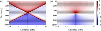
 $U_{0}=0.006~\text{m}~\text{s}^{-1}$
and
 $N=0.0017~\text{rad}~\text{s}^{-1}$
. Subinertial solutions are evanescent and trapped to the ridge crest with a decay scale
 $1/\hat{k}$
that decreases with latitude. Superinertial solutions are radiating waves with wavenumbers
 ${\check{k}}$
, and form characteristic internal wave beams at slopes determined by the dispersion relation. At
 $x=0$
the subinertial buoyancy field has a quadrature phase relationship with the barotropic tide, indicating that the largest isopycnals at the ridge occur during slack tide. Conversely, the superinertial buoyancy field is in phase, and peak isopycnal displacements are associated with peak cross-ridge flows.
Horizontal velocities non-dimensionalized by
 $U_{0}$
(colour) and isopycnals (contours) at
 $t=0$
for (a) superinertial (
 $f_{10^{\circ }}$
) and (b) subinertial (
 $f_{50^{\circ }}$
) solutions.

2.3 Energetics
Using the expressions obtained in the previous section, we evaluate the time and depth mean kinetic and potential energy at the ridge-crest (
 $x=0$
) using the following definitions appropriate for hydrostatic dynamics:
 $$\begin{eqnarray}\left.\begin{array}{@{}c@{}}\displaystyle \overline{\text{KE}}=\frac{{\it\rho}_{0}}{2}\frac{1}{Th}\int _{0}^{T}\int _{0}^{h}(u^{2}+v^{2})\,\text{d}z\,\text{d}t,\\ \displaystyle \overline{\text{APE}}=\frac{{\it\rho}_{0}}{2N^{2}}\frac{1}{Th}\int _{0}^{T}\int _{0}^{h}b^{2}\,\text{d}z\,\text{d}t.\end{array}\right\}\end{eqnarray}$$
The integrals are evaluated over the full water depth, capturing the energy associated with the response on the flank of the ridge as well as above its crest. The superinertial energies are
 $$\begin{eqnarray}\left.\begin{array}{@{}c@{}}\displaystyle \check{\overline{\text{KE}}}=\frac{1}{8}{\it\rho}_{0}U_{0}^{2}\left(\frac{{\it\omega}^{2}+f^{2}}{{\it\omega}^{2}}\right)\mathop{\sum }_{n=1}^{\infty }PP_{n}^{2},\\ \displaystyle \check{\overline{\text{APE}}}=\frac{1}{8}{\it\rho}_{0}U_{0}^{2}\left(\frac{{\it\omega}^{2}-f^{2}}{{\it\omega}^{2}}\right)\mathop{\sum }_{n=1}^{\infty }PP_{n}^{2},\end{array}\right\}\end{eqnarray}$$
and the subinertial energies are
 $$\begin{eqnarray}\left.\begin{array}{@{}c@{}}\displaystyle \hat{\overline{\text{KE}}}=\frac{1}{8}{\it\rho}_{0}U_{0}^{2}\left(\frac{{\it\omega}^{2}+f^{2}}{{\it\omega}^{2}}\right)\mathop{\sum }_{n=1}^{\infty }PP_{n}^{2},\\ \displaystyle \hat{\overline{\text{APE}}}=\frac{1}{8}{\it\rho}_{0}U_{0}^{2}\left(\frac{f^{2}-{\it\omega}^{2}}{{\it\omega}^{2}}\right)\mathop{\sum }_{n=1}^{\infty }PP_{n}^{2}.\end{array}\right\}\end{eqnarray}$$
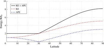
Figure 3 illustrates the strong influence of rotation on the ridge-top energies for a 24 h tide with a fixed tidal amplitude
 $U=0.006~\text{m}~\text{s}^{-1}$
, a stratification of
 $N=0.0017~\text{rad}~\text{s}^{-1}$
(1 cph), in a depth of 1000 m for a ridge of height 500 m. Below the turning latitude, the total energy density at the ridge has a fixed value of
 $2\times$
that of the barotropic tide for this particular choice of parameters. At
 $f_{0^{\circ }}$
this corresponds to a wavelike response with equipartitioned kinetic and potential energy. At higher latitudes the waves have a reduced potential energy, but an increased kinetic energy due to the along-ridge component whose speed increases with latitude as
 $f/{\it\omega}$
. Above the turning latitude the response is evanescent, but the along-ridge oscillatory currents continue to grow with latitude. In contrast to superinertial behaviour, the available potential energy of the evanescent response also grows with latitude as isopycnal displacements in the near field become large. The result is that for a fixed-amplitude barotropic tide, the ridge-crest energy density of the response increases with latitude once the flow is subinertial.
The increase in energy density with latitude also holds if the near-ridge, rather than ridge-crest, response is considered. Defining ‘near-ridge’ as within a distance of
 $k^{-1}$
from the crest, and using the dispersion relations in (2.16), we see that lengthscale of the response decreases linearly in
 $f$
. However, the ridge-top energy increases as
 $f^{2}$
, causing the total near-ridge energy of the response to increase with latitude.
Depth- and time-averaged kinetic and available potential energies at
 $x=0$
as a function of latitude, from theory.

Despite the elevated near-topographic energy densities above the turning latitude, in this inviscid, two-dimensional analytical model there is no conversion of energy from the barotropic tide to the baroclinic response once the latitude is subinertial. In the absence of dissipation, conversion may only arise by the generation of radiating waves, whose phase-averaged energy flux is defined:
 $$\begin{eqnarray}J=\frac{1}{T}\int _{0}^{T}\int _{0}^{h}\boldsymbol{u}p\,\text{d}z\,\text{d}t.\end{eqnarray}$$
In the subinertial solution, pressure and cross-ridge velocity have a quadrature phase relation in time and as a result there is no outward radiating flux, in contrast to the superinertial solution where the pressure and cross-ridge velocity are in phase. However, in the subinertial solution pressure and along-ridge velocity are in phase, suggesting the potential for along-ridge radiation in a three-dimensional solution.
3 Numerical simulations
3.1 Set-up
To test the above theory and explicitly illustrate the effects of changing latitude on tidal flows over topography, we use the MITgcm (Marshall et al.
Reference Marshall, Adcroft, Hill, Perelman and Heisey1997) and solve the full nonlinear, non-hydrostatic equations for two-dimensional tidal flow over a steep Gaussian seamount on an
 $f$
-plane. For all runs we set the tidal period to be 24 h, and the Gaussian topography to have a height of 500 m in 1000 m of water, and a horizontal e-folding scale of 1000 m. Stratification is constant in depth with a Brunt–Väisälä period of 1 h (
 $N=0.0017~\text{rad}~\text{s}^{-1}$
).
For the finite width bathymetry in these simulations, a measure of the linearity of the flow is given by a non-dimensional excursion length
 $$\begin{eqnarray}{\it\varepsilon}_{rdg}=\frac{U_{c}}{{\it\omega}l_{rdg}},\end{eqnarray}$$
which compares the horizontal displacement of a fluid parcel each tidal cycle (
 $l_{exc}=U_{c}/{\it\omega}$
) to a characteristic width of the ridge (
 $l_{rdg}$
). Here
 $U_{c}$
is the depth mean speed at the crest of the topography. Simulations are divided into two categories: the small excursion length simulations have a very small-amplitude barotropic tide (
 $U_{0}=0.006~\text{m}~\text{s}^{-1}$
), and the long excursion length simulations have a larger-amplitude tide (
 $U_{0}=0.02~\text{m}~\text{s}^{-1}$
). Generating tidal excursion lengths at the ridge crest of 160 and 550 m, respectively. An appropriate characteristic ridge width is determined at a depth from the crest determined by the vertical length scale associated with the flow:
 ${\it\delta}=U_{c}/N$
(Winters & Armi Reference Winters and Armi2013). For these parameters, we estimate the characteristic ridge widths to be 240 and 430 m, respectively. As such, the small excursion length simulations have
 ${\it\varepsilon}_{rdg}<1$
, and the large excursion length simulations have
 ${\it\varepsilon}_{rdg}>1$
.
A second important parameter is the topographic Froude number, which is defined as
 $$\begin{eqnarray}Fr=\frac{U_{0}}{Nz_{0}}.\end{eqnarray}$$
All simulations presented in this study have very small values of
 $Fr$
, which in the ocean corresponds to tall topography where most of the tidal flow is unable to surmount the crest during all phases of the tide. Much of the tidal transport above the crest is accommodated in a relatively fast, thin, bottom intensified layer (Winters & Armi Reference Winters and Armi2013).
In these simulations the topography is supercritical at all latitudes where the tide is superinertial, meaning that it is steeper than the characteristics of the fundamental frequency internal wave response. The barotropic tide is approximated in the model by the addition of a spatially uniform body force
 $(G_{u},G_{v})$
to each of the horizontal momentum equations such that in the absence of topography the flow is rectilinear in the
 $x$
-direction and oscillatory with frequency
 ${\it\omega}$
and amplitude
 $U_{0}$
(Di Lorenzo, Young & Llewellyn Smith Reference Di Lorenzo, Young and Llewellyn Smith2006). Specifically, we set
 $$\begin{eqnarray}(G_{u},G_{v})=(-U_{0}{\it\omega}\sin ({\it\omega}t),U_{0}f\cos ({\it\omega}t)).\end{eqnarray}$$
In the real ocean, the barotropic tide itself may be subject to dynamics including subinertial trapping (Longuet-Higgins Reference Longuet-Higgins1968), however, its lengthscales are typically determined by the barotropic Rossby radius, of order 1000 km. As these scales are much larger than those being considered here, our spatially uniform approximation of the tide in these simulations is justified. The inclusion of a more realistic background tidal ellipse does not change the dynamics of these two-dimensional simulations, but it imposes greater computational demand by restricting the time step. Eleven small excursion length simulations are presented with
 $f$
corresponding to latitudes,
 ${\it\theta}=[0,10,20,25,35,40,50,60,70,80,90]^{\circ }$
. We use subscript notation to refer to each simulation, where, for example,
 $f_{50^{\circ }}$
indicates the simulation was performed at a latitude of
 $50^{\circ }$
. Two large excursion length simulations are performed at
 $3.85^{\circ }$
and
 $44.7^{\circ }$
. These latitudes are chosen because the theory of § 2 predicts that the amplitude of near-crest isopycnal displacement, and therefore the available potential energy at the ridge crest, will be the same at each, even though the nature of the response will be fundamentally different. At
 ${\it\theta}=30^{\circ }$
we are very close to the turning latitude of a 24 h tide and the lengthscale,
 $k^{-1}$
, is too large to fit in the computational domain, therefore we do not present results from this simulation.
We telescope our grids in the horizontal such that resolution is highest within 30 km of the ridge. Small excursion length simulations have an isotropic resolution of 15 m, and large excursion length simulations have an isotropic resolution of 5 m within this high-resolution region. In all cases, the domain has a total width of 300 km and is horizontally periodic. Baroclinic signals that reach the boundaries reenter the domain at the opposite boundary at a time determined by the phase speed of the signals and the width of the computational domain. We define an analysis region within
 $\pm$
4 km of the ridge crest, and perform all analysis before these spurious signals reach the boundaries of our analysis domain, which occurs at a time easily identified using Hovmöller diagrams at fixed depth. For these simulations we have determined that between 120 and 144 h, five periods after the simulation starts, flows in the analysis region are uncontaminated by these reentrant waves.
As a check on the convergence of our numerical solutions, two of the small excursion length simulations (
 $f_{10^{\circ }}$
and
 $f_{50^{\circ }}$
) are repeated with identical parameters but doubled resolutions to ensure that our solutions are not quantitatively resolution dependent. Evaluation of the kinetic energy budget in the double-resolution simulations reveal differences of less than 3 % in the dominant terms, giving us confidence in the quantitative results of our standard-resolution simulations. We achieve good closure of the budget in the higher-resolution long excursion length simulations, where time mean residuals in the energy balance are approximately four times smaller than the smallest term in the kinetic energy budget (the dissipation rate). Closure of the budget in the small excursion length simulations have residuals that are comparable with computed dissipation rates, which themselves comprise around 1 % of the largest terms in the budget. Residuals in this budget arise from spatial and temporal discretization errors in our post-simulation evaluation of the terms, in addition to numerical diffusion by the model numerical schemes.
The small excursion length simulations were performed with constant background viscosities of
 $2\times 10^{-3}~\text{m}~\text{s}^{-2}$
corresponding to Reynolds numbers between 1500 and 5000, though the simulations are non-turbulent. The high-resolution long excursion length simulations additionally employ a Smagorinsky turbulence closure (Smagorinsky Reference Smagorinsky1963), with a Smagorinsky coefficient of
 $C_{s}^{2}=0.03$
. Diffusivities are
 $8\times 10^{-4}~\text{m}~\text{s}^{-2}$
for all simulations, and no-slip boundary conditions are enforced at the topography. To minimize numerical diffusion, a seventh-order monoticity preserving scheme is used for tracer advection (Daru & Tenaud Reference Daru and Tenaud2004). Momentum advection is by a centred second-order scheme.
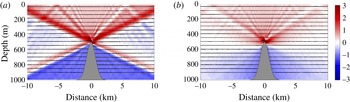
Widefield snapshots of
 $u$
, with isopycnals contoured, for small excursion length simulation at (a)
 $f_{10}$
, where the fundamental frequency response is radiating, and (b)
 $f_{50}$
, where the fundamental frequency response is evanescent. Spatially constant background tide,
 $u_{b}$
, has been removed. Non-dimensionalized by
 $U_{0}$
.

Snapshots of
 $u$
(a) and
 $v$
(b) with isopycnals (contoured) for small excursion length simulation at
 $f_{10}$
, where the fundamental frequency response is radiating. Background tide,
 $u_{b}$
, has been removed. Non-dimensionalized by
 $U_{0}$
.

Snapshots of
 $u$
(a) and
 $v$
(b) with isopycnals (contoured) for small excursion length simulation at
 $f_{50}$
, where the fundamental frequency response is evanescent. Background tide,
 $u_{b}$
, has been removed. Non-dimensionalized by
 $U_{0}$
.

3.2 Small excursion length simulations
3.2.1 Flow snapshots
Widefield snapshots of cross-ridge flow at 120 h are presented in figure 4 for the simulations at latitudes of
 $10^{\circ }$
and
 $50^{\circ }$
. In this and all subsequent snapshot figures the spatially constant background tide,
 $u_{b}$
, has been removed. Parameters are the same as used in the linear analytic solution presented in figure 2, enabling a direct comparison of linear theory with model output. In the
 $f_{10^{\circ }}$
simulation, the forcing frequency is superinertial and the domain is filled with baroclinic energy associated with energetic radiating internal tides. Beams are present, formed from the superposition of linear internal wave modes. Their angles are dependent upon wave frequency according to the internal wave dispersion relation. Harmonics of the forcing frequency are visible at steeper angles, arising due to advection by the background tide (Bell Reference Bell1975). In contrast, the subinertial
 $f_{50^{\circ }}$
simulation has much less energy in the far field as energy at the forcing frequency is unable to radiate at this latitude. Beams at angles corresponding to harmonics of the fundamental frequency are present, indicating the generation of some radiating energy, however, their energy content is small.
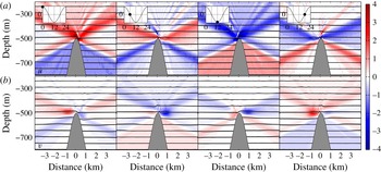
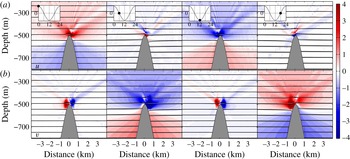
Nearfield snapshots of the simulations at 6 h intervals between 120 and 138 h are shown in figures 5 and 6. Cross-ridge velocity,
 $u$
, is presented in the upper panel, and along-ridge velocity,
 $v$
, in the lower panel. Consistent with the linear solution, velocities in the along-ridge direction have an amplitude of
 $fU_{0}/{\it\omega}$
and are therefore much smaller at
 $10^{\circ }$
(figure 5) than at
 $50^{\circ }$
(figure 6). In the
 $f_{50^{\circ }}$
simulation, the quadrature phase relation between displacement and cross-ridge velocity is evident as isopycnal displacements occur with a 6 h lag behind cross-ridge flows. In agreement with the theory of § 2, both along- and cross-ridge velocities are baroclinic away from topography. The periodic nature of the symmetric tidal flow is demonstrated as the third and fourth panels are mirror images of the first and second panels, with the colors reversed. Time mean along-ridge jets form along the flanks of the ridge and are most clearly visible at 0 and 12 h of the snapshots, and are discussed in detail in the next section.
3.2.2 Phase-averaged flows
Despite the small amplitudes of the tide in these simulations, nonlinear effects generate significant rectified along-ridge flows near the crest of the ridge whose magnitude increases with latitude. In the deep ocean, tidally rectified flows arise under the combined influence of a Stokes drift associated with the Coriolis turning of a fluid parcel as it changes its water depth, and an Eulerian mean current (Huthnance Reference Huthnance1973; Loder Reference Loder1980). In the shallow water near the ridge crest, continuity and Coriolis turning cause the tidal ellipse to be larger than in deeper water. The tidal Stokes drift arises as fluid parcels advected between deep and shallow water each tidal cycle experience asymmetric along-ridge flows, leading to a time-mean drift along the ridge (in the northern hemisphere the drift is with shallow water to the left). However, in the shallow water close to the crest fluid parcels experience greater friction than in deeper water, and an Eulerian mean flow is established such that, combined with the Stokes drift, fluid parcels experience no time mean accelerations or drag over each tidal cycle. The Eulerian mean flow is in the opposite sense to the Stokes drift such that along-ridge parcel velocity is enhanced in low friction (deeper) regions relative to high friction (shallower) regions, and the net drag is zero. The resulting mean Lagrangian current is in the same sense as the Eulerian current (shallow water to the right, in the northern hemisphere), but is smaller due to the influence of the mean Stokes velocity. The generation of these flows has been studied for a stratified fluid over small-amplitude topography in some detail (Maas & Zimmerman (Reference Maas and Zimmerman1989a ) and Maas & Zimmerman (Reference Maas and Zimmerman1989b ), hereafter MZ88a and MZ88b, respectively). MZ88b find that stratification causes the rectified flows to be bottom trapped, and associated with Eulerian mean cross-isobath circulations. In this section we illustrate these flows in our simulations from both the Eulerian and Lagrangian reference frame and find good qualitative agreement between the small-amplitude topography theory presented in MZ88b, and the rectified flows occurring in these finite-amplitude topography simulations.
Eulerian mean along-ridge velocities normalized by
 $U_{0}$
at (a)
 $f_{10^{\circ }}$
and (b)
 $f_{50^{\circ }}$
. Grey contours are
 $x{-}z$
streamfunction. (c) Depth mean along-ridge velocities from all small excursion length simulations. Higher latitudes are darker, with purples indicating superinertial latitudes and greens indicating subinertial latitudes.

Eulerian time-mean along-ridge currents (colour),
 $x{-}z$
streamfunction (grey contours) and isopycnal displacements (black contours) from the analysis period for the simulations at
 $f_{10^{\circ }}$
and
 $f_{50^{\circ }}$
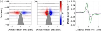
are shown in figure 7(a,b). The Eulerian mean streamfunction is computed by integrating the time mean cross-ridge component in
 $z$
, with the integration constant set to ensure continuity over the ridge. In all simulations with
 $f\neq 0$
, a mean flow develops that is predominantly composed of a pair of along-ridge jets with anticyclonic vertical vorticity at the ridge crest, with a general trend that the jets become faster as latitude increases (figure 7
c). Peak jet speeds in the
 $f_{50^{\circ }}$
simulation are in excess of
 $3U_{0}$
and are located at around the depth of the crest of the topography (note that at this latitude the oscillatory along-ridge response has a magnitude of
 $fU_{0}/{\it\omega}=1.5U_{0}$
). As predicted in MZ88b, these Eulerian time-means exhibit secondary circulations in the
 $x{-}z$
plane: jet-centred cells with peak downwards velocities of around 0.25
 $U_{0}$
at the crest, and weaker upward velocities near the outside of each of the jets. The phase mean along-ridge jets in the
 $f_{10^{\circ }}$
simulation are weaker and extend further in the horizontal.
Depth mean near-ridge (a,c,e)
 $x$
-momentum budget (non-dimensionalized by
 $fU_{0}$
) and (b,d,f) buoyancy budget (non-dimensionalized by
 $w_{0}N^{2}$
) for
 $f_{50^{\circ }}$
. Thick lines in upper panels indicate the dominant balance in the equations. Lower panels break down the advective terms into perturbations and means.

We compute the Eulerian mean momentum balance by performing a Reynolds decomposition of the fields such that they are composed of three parts: an Eulerian phase-averaged component (angle brackets), the oscillatory baroclinic response component (primes), and, in the case of the cross-ridge velocity, the spatially uniform background tide (
 $u_{b}$
):
 $$\begin{eqnarray}\left.\begin{array}{@{}c@{}}u=\langle u\rangle +u^{\prime }+u_{b};\quad v=\langle v\rangle +v^{\prime };\quad w=\langle w\rangle +w^{\prime },\\ p=\langle p\rangle +p^{\prime };\quad b=\langle b\rangle +b^{\prime }.\end{array}\right\}\end{eqnarray}$$
These expressions are substituted into the nonlinear equations of motion, and averaged over one tidal period:
 $$\begin{eqnarray}\displaystyle \left.\begin{array}{@{}c@{}}\langle u\rangle _{t}+\langle p\rangle _{x}-f\langle v\rangle -{\it\nu}{\rm\nabla}^{2}\langle u\rangle =-(\langle u_{b}u^{\prime }\rangle _{x}+\langle u^{\prime }u^{\prime }\rangle _{x}+\langle w^{\prime }u^{\prime }\rangle _{z}+\langle u\rangle \langle u\rangle _{x}+\langle w\rangle \langle u\rangle _{z}),\\ \langle v\rangle _{t}+f\langle u\rangle -{\it\nu}{\rm\nabla}^{2}\langle v\rangle =-(\langle u_{b}v^{\prime }\rangle _{x}+\langle u^{\prime }v^{\prime }\rangle _{x}+\langle w^{\prime }v^{\prime }\rangle _{z}+\langle u\rangle \langle v\rangle _{x}+\langle w\rangle \langle v\rangle _{z}),\\ \langle w\rangle _{t}+\langle p\rangle _{z}-\langle b\rangle -{\it\nu}{\rm\nabla}^{2}\langle w\rangle =-(\langle u_{b}w^{\prime }\rangle _{x}+\langle u^{\prime }w^{\prime }\rangle _{x}+\langle w^{\prime }w^{\prime }\rangle _{z}+\langle u\rangle \langle w\rangle _{x}+\langle w\rangle \langle w\rangle _{z}),\\ \langle b\rangle _{t}+N^{2}\langle w\rangle -{\it\kappa}{\rm\nabla}^{2}\langle b\rangle =-(\langle u_{b}b^{\prime }\rangle _{x}+\langle u^{\prime }b^{\prime }\rangle _{x}+\langle w^{\prime }b^{\prime }\rangle _{z}+\langle u\rangle \langle b\rangle _{x}+\langle w\rangle \langle b\rangle _{z}),\\ \langle u\rangle _{x}+\langle w\rangle _{z}=0.\end{array}\right\} & & \displaystyle \nonumber\\ \displaystyle & & \displaystyle\end{eqnarray}$$
The advective terms are grouped on the right-hand side of the equations, and represent forcing terms for the Eulerian mean fields. Three types of nonlinear interaction can give rise to a momentum flux into the Eulerian mean: (1) self-interaction of the primed fields (Reynolds stresses); (2) self-interaction of the mean fields; and (3) interaction of the barotropic tide with the primed fields. Terms making up the momentum and buoyancy budgets were computed at the beginning of the fifth period for the double-resolution simulation at
 $f_{50^{\circ }}$
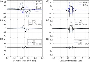
in a region close to the crest of the ridge. The across-ridge momentum and buoyancy budgets and are shown in figure 8, where (a,b) shows the dominant terms and budget residual. All of the nonlinear terms are included in
 $\langle \text{D}u/\text{D}t\rangle$
and
 $\langle \text{D}b/\text{D}t\rangle$
, respectively.
Consistent with the expected balance for tidally rectified flows (e.g. Loder Reference Loder1980), the across-ridge (
 $x$
) momentum balance for the Eulerian mean flow is predominantly in geostrophic balance (figure 8
a, pale blue dashed and grey solid lines), with a residual supported by nonlinear terms. The terms corresponding to the rate of change of the mean cross-ridge flow and viscous diffusion of mean
 $x$
-momentum were found to be negligibly small compared with the other terms and are not explicitly shown (the time dependent terms make a small contribution to
 $\langle \text{D}u/\text{D}t\rangle$
and
 $\langle \text{D}b/\text{D}t\rangle$
). The nonlinear terms are broken down in figure 8(c–f), and show that the dominant terms are the Reynolds stresses, shown in figure 8(c).
Terms in the Eulerian buoyancy budget are shown in figure 8(b). Figure 8(a,b) illustrates the balance between nonlinear terms and the Eulerian vertical velocity. Once again, the time derivative and diabatic terms are small compared with the others and are not shown. The smallness of the diffusive term confirms that despite the relatively large Eulerian vertical velocities, fluid parcels do not cross isopycnals in the time mean, underscoring the importance of a Lagrangian frame of reference when considering time mean fluid motion in oscillatory flows. Eulerian mean vertical velocities are mainly supported by Reynolds stresses (figure 8 d), and to a lesser extent by interactions of the Eulerian mean fields (figure 8 f).
Particle trajectories over one period for 9 particles seeded at 120 h in
 $f_{50^{\circ }}$
simulation: (a) side view; (b) plan view. Green tracks are for particles seeded at
 $-$
480 m, red tracks are particles seeded at
 $-$
520 m. Blue dots indicate starting positions.

Whilst the diabatic and unsteady terms are negligibly small in the across-ridge momentum and buoyancy budgets, they are small but non-zero in the along-ridge (
 $y$
) momentum balance (not shown), indicating that the jets are slowly accelerating at the time that the budget was diagnosed. Mixing results in a volume of intermediate density fluid close to the crest of the ridge that slowly increases over the course of the simulation (see § 3.3). Chen & Beardsley (Reference Chen and Beardsley1995) found similar processes to be occurring in their simulations of stratified tidal flow over a shallow two-dimensional ridge where it generated a tidal mixing front, which, through Rossby adjustment, became associated with a frontal jet. The generation of mixed fluid in our simulations provides a small but steadily increasing contribution to the rectified flows generated by Coriolis turning and friction.
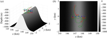
Individual particle trajectories were computed over one period for the flow as a post-processing step by integrating the 10 min output fields using a Runge–Kutta fourth-order scheme. Paths are dependent on the phase of the tide at which the particles were seeded, and figure 9 shows nine paths initiated at slack tide before eastward flow in the
 $f_{50^{\circ }}$
simulation. Particles close to the crest exhibit looping trajectories along the ridge, as they move under the combined influence of Stokes drift and the Eulerian mean flow, spending less time in shallower water (higher friction) than in deeper water (lower friction) such that they experience no net drag. Short-wavelength oscillations are apparent in some tracks as particles pass through nonlinear lee waves. Further away from the crest, particles exhibit tracks that are much more elliptical, and close to those expected from the zero-order linear solution. Particle tracks in the
 $f_{10^{\circ }}$
simulation (not shown) are qualitatively similar, but have smaller displacements along the ridge crest due to weaker rectified flows.
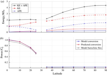
Energies averaged over 2 km region at ridge crest. (a) Thick lines: phase mean kinetic (red dashed), available potential (blue dashed) and total energy (black solid). Thin lines: kinetic (red) and available potential (blue) energy in the time mean flow. (b) Barotropic–baroclinic conversion from theory (red) and model (blue), and baroclinic flux out of region (grey).

3.2.3 Energetics
Tidal averages of kinetic and available potential energies in the region above the topography are shown in figure 10(a). The finite width of the model ridge makes a precise comparison with theory impossible, as such we present the spatial average in a region 2 km wide and centred at the crest of the ridge. For comparison with the theoretical results shown in figure 3, the kinetic energy is computed from only the velocity field arising from the presence of the topography, i.e. with the time-dependent but spatially constant background tide,
 $u_{b}$
, removed.
Consistent with theory, average ridge-crest energy is approximately constant below the turning latitude, but increases with latitude where the barotropic tide is subinertial. Where the tide is superinertial, the radiated wave field has a spatially constant energy density, and integrals over the analysis region compare well with the energy densities predicted by theory. However, when the tide is subinertial the response is spatially varying, and decays exponentially away from topography. In this case the influence of the finite width of the topography on the spatial average causes the measured energy density to be much smaller than that predicted for the knife-edge ridge.
Kinetic and potential energies associated with the Eulerian time mean flow are shown in thin lines in figure 10(a). Even though the phase-averaged flows have velocities comparable with the tidal amplitude, they constitute much less energy than their time-dependent counterparts due to their limited spatial extent. The amplitudes of these mean flows tends to increase with latitude up to
 $70^{\circ }$
and is roughly constant above that (figure 7).
Terms in the baroclinic energy budget are evaluated following (Kang & Fringer Reference Kang and Fringer2012) for the analysis region, and are shown in figure 10(b). The predicted rate of conversion of barotropic to baroclinic energy by a knife edge ridge with the same parameters (stratification, tidal amplitude and height) are also shown, and the conversion predicted at
 ${\it\theta}=0$
is used to non-dimensionalize all values (Llewellyn Smith & Young Reference Llewellyn Smith and Young2003). Modelled conversion is remarkably well predicted by the knife-edge model, despite the nonlinearities and finite width of the numerical simulation. Conversion decreases with latitude up to the turning latitude, and is negligible beyond, as the evanescent response does not extract energy from the barotropic tide in steady state. At superinertial latitudes, model baroclinic fluxes are comparable with conversion as most of the converted energy radiates out of the domain in the form of internal tides. Differences between the conversion and baroclinic flux arises from the dissipation of baroclinic energy within the domain. When the tide is subinertial, radiated fluxes are negligible, and all converted barotropic to baroclinic energy is dissipated locally.
3.3 Long excursion length simulations
Nearfield mixing can arise through both breaking tidal lee waves and transient hydraulic jumps (Musgrave et al.
Reference Musgrave, Mackinnon, Pinkel, Waterhouse and Nash2016), influencing the overall tide-topography energy budget by dissipating energy in the nearfield, and reducing the radiated internal wave flux (Klymak, Legg & Pinkel Reference Klymak, Legg and Pinkel2010; Rapaka, Gayen & Sarkar Reference Rapaka, Gayen and Sarkar2013). In this section we present the results of two simulations having relatively long excursion lengths (
 $l_{exc}\approx l_{rdg}$
), and contrast the development of nearfield mixing when the tide is subinertial, then superinertial. The tidal amplitudes of these flows are
 $0.02~\text{m}~\text{s}^{-1}$
, which is small, even in the deep ocean. Though the cross-ridge kinetic energy of the response is the same at all latitudes, the along-ridge kinetic energy and available potential energy depends on latitude. These simulations were performed at latitudes of
 $3.85^{\circ }$
and
 $44.7^{\circ }$
, where theory predicts that the amplitude of the ridge-top buoyancy anomaly (potential energy) will be the same, enabling as close to an equivalent comparison as possible.
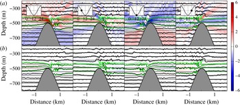
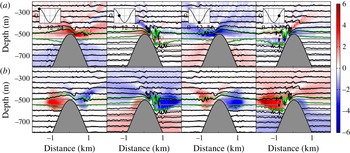
Snapshots of the flow at 6 h intervals during the fifth period of the simulation are shown in figures 11 (superinertial) and 12 (subinertial). As in the small excursion length simulations, the superinertial tide generates radiating energy at the fundamental frequency and its harmonics which forms beams at characteristic slopes emanating from the topographic crest. Close to the crest, the wavefield constructively superposes during peak cross-ridge flow to form tidal lee waves: time-dependent beam-like features that have slopes that change with the tide as the composite frequencies disperse (Bell Reference Bell1975; Musgrave et al. Reference Musgrave, Mackinnon, Pinkel, Waterhouse and Nash2016). The subinertial simulation has some energy at harmonics, but the response at the fundamental frequency is trapped and associated with large-amplitude along-ridge flows. The quadrature phase relation between ridge-top flow and isopycnals is more obvious in these large-amplitude simulations, with the subinertial simulation having large isopycnal displacements during slack tide (hours 6 and 18). In hours 0 and 12, isopycnals very close to the crest of the ridge on its upstream side exhibit vertical displacements that are not predicted by the linear theory in § 2, and are associated with the phase-averaged jets.
Snapshots of cross-ridge velocity
 $u$
(a) and along-ridge velocity
 $v$
(b) with isopycnals (contoured) for nonlinear simulation (
 $U_{0}=0.02~\text{m}~\text{s}^{-1}$
) at
 $f=3.85^{\circ }$
, where the fundamental frequency response is radiating. Green contours indicate temperature classes which have increased in volume through mixing.

Snapshots of cross-ridge velocity
 $u$
(a) and along-ridge velocity
 $v$
(b) with isopycnals (contoured) for nonlinear simulation (
 $U_{0}=0.02~\text{m}~\text{s}^{-1}$
) at
 $f=44.7^{\circ }$
, where the fundamental frequency response is evanescent. Green contours indicate temperature classes which have increased in volume through mixing.

Area integrated dissipation rates within
 $\pm 4$
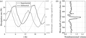
km of the ridge crest are presented for each simulation during the fifth period in figure 13(a). In these two-dimensional simulations, computed dissipation rates are not representative of dissipation associated with fully turbulent, three-dimensional flows at high Reynolds number. Nevertheless, their relative values and timings provide insight on which of the two simulations are more dissipative, and when during the tidal cycle the dissipation occurs. Dissipation rates take larger values and peak later in the tidal cycle for the subinertial simulation compared with the superinertial simulation. In the superinertial simulation tidal transport is in phase with isopycnal displacement at the ridge crest, and peak dissipation lags peak tidal flow by around an eighth of a period as dissipative processes in the hydraulic jump continue to grow even once the cross-ridge tidal transport starts to decrease. In the subinertial simulation isopycnal displacement lags tidal transport by a quarter period at the ridge crest, and peak dissipation rates are both larger than in the superinertial simulation, and lag peak tidal flow by almost a quarter of a period, occurring significantly later in the tidal cycle than in the superinertial case. As the cross-ridge transport relaxes, the combination of upward-moving isopycnals on the upstream side, and downward moving isopycnals on the lee side causes the near-bottom, hydraulically controlled jet to persist for longer, with the hydraulic jump developing in a region of relatively low stratification (associated with large isopycnal displacement) and generating a more dissipative hydraulic jump than in the superinertial case. In the latter situation, the relaxing tidal transport is associated with increasing downstream stratification.
(a) Integrated dissipation rate within
 $\pm 4$
km of the crest versus time during the fifth period. Thin dashed line is background tide,
 $u_{b}$
. (b) Volume of fluid occupied by given temperature class at 120 h, non-dimensionalized by volume occupied at 0 h.

We assess the vertical distribution of mixing in each simulation within the analysis domain (
 $\pm 4$
km of the ridge crest) by defining an evenly spaced set of temperature classes, then computing the volume of fluid occupied by each temperature class at the beginning of the simulation, and at 120 h of the simulation. Figure 13(b) shows the volume of fluid occupied by each temperature class, non-dimensionalized by its initial volume for both the sub- and superinertial simulations. Volumes different than one indicate that diabatic processes have mixed fluid into or out of that temperature class. Both simulations show distinct mixing peaks at depths of
 ${\sim}500$
m, corresponding to relatively weakly stratified fluid that develops close to the peak. Adjacent temperature classes occupy a reduced volume of fluid, indicating relatively high stratifications surrounding the mixed fluid. The superinertial simulation has a second, smaller peak at around 430 m depth. The temperature classes which have grown (non-dimensional volumes greater than one) are outlined in green contours in figures 11 and 12. Musgrave et al. (Reference Musgrave, Mackinnon, Pinkel, Waterhouse and Nash2016) distinguish between mixing arising from hydraulic jump-like features which occur on the flanks of topography, and mixing arising from convective instability of the radiating lee wave component, which occurs at shallower depths, mainly above the ridge crest. The lack of a second, shallower peak in the subinertial simulation is consistent with the evanescent (non-radiating) fundamental frequency response, and consequently a much smaller radiating component than in the superinertial case. The dominant mixing mechanism here is a transient hydraulic jump of the bottom trapped cross-ridge jet, forming on the flanks of the ridge each tidal cycle. In the superinertial simulation, the constructive interference of the fundamental and harmonic responses is of large enough amplitude to generate breaking and mixing in a radiating tidal lee wave, forming a second, smaller peak in mixing above the top of the ridge. It is notable that the subinertial simulation is more dissipative, despite the relative contribution from the radiating component being much smaller in this case.
4 Trapped internal tides in three dimensions
The distinctly different nature of the evanescent compared with the radiating response results in changes not only to the magnitude and spatial distribution of tidal energy near topography, but also the timing, structure and evolution of nearfield tidally driven mixing. In addition, nonlinear effects generate fast along-ridge time mean currents, even when tidal amplitudes are small. A natural question that arises is to what extent these idealized two-dimensional results apply in a more general three-dimensional setting, and whether additional phenomena may become important.
Our imposition of two-dimensional solutions excludes a priori features with along-ridge variation, including trapped topographic waves, which have been observed at several high-latitude locations (Padman et al. Reference Padman, Plueddemann, Muench and Pinkel1992; Kunze & Toole Reference Kunze and Toole1997). The structure of these trapped waves can be determined for specific topographies and stratifications by numerically solving an eigenvalue problem whose eigenmodes correspond to the resonant modes of the topography (Huthnance Reference Huthnance1978; Brink Reference Brink1989; Codiga Reference Codiga1997). Trapped modes have discrete subinertial frequencies, and propagate anticyclonically around bathymetry. When the eigenfrequencies of the trapped modes are close to that of a tidal constituent, trapped tides at that frequency may be resonantly excited, generating relatively large-amplitude tidal currents close to the topography (Chapman Reference Chapman1989). Unlike the two-dimensional forced solutions discussed in this paper, the eigenmodes corresponding to trapped tides are constructed such that they individually satisfy a boundary condition of no-flow through the boundary. Conversely, in the forced tidal problem, solutions are required to add to the background tide such that there is no flow through the boundary, which means that the solutions themselves have a component perpendicular to the boundary. Despite this distinction, we note that in the subinertial solution, the phase relation between displacement and along-ridge flow is consistent with propagation along the ridge (if along-ridge variation was allowed). As a result, the forced response described in this paper will resonantly excite the trapped eigenmodes of the topography if the topographic length scales and ambient stratification are such that the eigenfrequencies of the topography are close to the forcing frequency. For isolated topographies, the potential for such resonant forcing may have important consequences for nearfield mixing and dissipation, as a large-amplitude response is subject to nonlinearities and breaking.
Even in the absence of a resonance between the forced response and the eigenmodes of the topography, we expect that the characteristics of the subinertial forced solutions described here are relevant in three dimensions, generating strong along-ridge flows that are phase locked with the background tide and having displacements and velocities that increase, and off-ridge length scales that decrease at higher latitudes.
5 Discussion and conclusions
In this paper we have examined the two-dimensional response of a stratified ocean to subinertial tidal forcing, and contrasted it to the relatively well-studied response to superinertial tidal forcing. Analytic solutions for a tall, infinitely thin barrier predict a latitudinal increase in the energy density at the ridge-crest when the tide is subinertial, arising from large along-ridge flows and isopycnal displacements. This is confirmed in a series of numerical simulations, which additionally illustrate the distinctive evanescent nature of the response. The elevated energy density of near-ridge subinertial tidal flows may strongly influence regional mixing at high latitudes, affecting critical climate processes including ice melt and ocean–atmosphere heat exchange.
All simulations with
 $f\neq 0$
generate along-ridge rectified currents, demonstrating the importance of nonlinearity in these flows despite the small barotropic amplitudes. The speed of the Eulerian mean currents increase with latitude, with peak speeds reaching
 $4u_{0}$
at latitudes of
 $80^{\circ }$
, though the jet speeds continue to increase during our simulations. The time mean flows are primarily associated with the Coriolis mechanism described by Huthnance (Reference Huthnance1973), whereby Coriolis turning and frictional drag cause fluid parcels to acquire relative vorticity. Additional routes for nearfield dissipation may be associated with these currents in three dimensions, either by interaction with along-bathymetric features which could lead to along-ridge hydraulic processes, or even via the generation of Kelvin–Helmholtz-type instabilities. Using the Eulerian mean field at
 $f_{50^{\circ }}$
, and with
 $N=1$
cph, we estimate a vertical shear of
 ${\sim}9\times 10^{-4}~\text{s}^{-1}$
, which results in a Richardson number of around 3.7. However, the influence of nearfield mixing on locally reducing stratification, combined with time-dependent changes in shear and stratification has the potential to reduce the Richardson number during some phases of the tide such that instabilities in the along-ridge flow may play an important role. In addition, the Lagrangian transport associated with these jets may be important for high-latitude coastal processes, transporting and mixing water masses across the shelf-break and providing a pathway for the regional transport of tracers and biological material (Flexas et al.
Reference Flexas, Schodlok, Padman, Menemenlis and Orsi2015).
A pair of simulations with larger-amplitude tides (
 $0.02~\text{m}~\text{s}^{-1}$
) at latitudes that are superinertial and subinertial for the 24 h tide show that the subinertial simulation is relatively more dissipative, with peak dissipation occurring around
 ${\rm\pi}/2$
after peak barotropic velocity in the subinertial case, compared to around
 ${\rm\pi}/4$
in the superinertial case. Enhanced mixing in the subinertial simulation is due to reduced stratification downstream of the crest when the transient hydraulic jump is developing. The vertical distribution of mixing in both simulations is similar, though the superinertial simulation has more mixing higher in the water column, associated with the radiating lee wave response. In both simulations, most of the mixing occurs on the near-crest flanks of the ridge, and is associated with hydraulic control of a bottom intensified cross-ridge jet.
The generation of evanescent wave responses is not restricted to subinertial frequencies. Maas (Reference Maas2011) shows that certain topographic shapes may be expected to generate evanescent baroclinic signals at specific frequencies, even when the tidal forcing is superinertial. As such, the enhanced nearfield mixing that we observe in this study may have a broader relevance to superinertial evanescent responses.
The idealized nature of this study invites further, more realistic investigation. In particular, the influence of three-dimensional topography and a varying stratification are relevant in an oceanic context. Our restriction to constant stratification is applicable in the deep ocean, where a trapped response may not extend as far as a pycnocline. However, in shallow water this is not the case, and an understanding of how variations in stratification might affect the solution may be important. The effects of three-dimensional topography, and particularly the interaction of the forced response discussed here with three-dimensional trapped subinertial free modes may lead to significantly more nearfield dissipation and mixing compared with when the tide is superinertial. This additional complexity may indicate that parametrizing the dissipation of subinertial tidal constituents may prove more complicated than their superinertial counterparts.
Acknowledgements
We thank N. Grisourd for helpful discussions relating to this work, and M. Nikurashin for help setting up the numerical model. Computing was performed on the Yellowstone Supercomputer, NSF award number ANT-0961218. R.C.M. acknowledges funding from the Office of Naval Research under grant ONR N00014-12-1-0943 and from the National Science Foundation under grant NSF OCE 1129763. M.M. acknowledges the National Science Foundation (NSF) for support of this research through grants OCE-1234473 and PLR-1425989.