1 Introduction
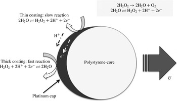
In recent years there has been a flurry of activity in developing micro- and nanoscale self-propelling devices that are engineered to produce enhanced motion within a fluid environment (Kapral Reference Kapral2013). They are of interest for a number of reasons, including the potential to perform transport tasks (Patra et al. Reference Patra, Sengupta, Duan, Zhang, Pavlick and Sen2013) and exhibit new emergent phenomena (Volpe et al. Reference Volpe, Buttinoni, Vogt, Kümmerer and Bechinger2011; Theurkauff et al. Reference Theurkauff, Cottin-Bizonne, Palacci, Ybert and Bocquet2012; Bricard et al. Reference Bricard, Caussin, Desreumaux, Dauchot and Bartolo2013; Kümmel et al. Reference Kümmel, ten Hagen, Wittkowski, Buttinoni, Eichhorn, Volpe, Löwen and Bechinger2013; Marchetti et al. Reference Marchetti, Joanny, Ramaswamy, Liverpool, Prost, Rao and Simha2013; Palacci et al. Reference Palacci, Sacanna, Steinberg, Pine and Chaikin2013). A variety of subtly different methods, all based on the catalytic decomposition of dissolved fuel molecules, have been shown to produce autonomous motion or swimming. Commonly studied systems are catalytic bimetallic rod-shaped devices (Kline et al. Reference Kline, Paxton, Wang, Velegol, Mallouk and Sen2005b ) and metallic-insulator spherical Janus particles that are half-coated with catalyst (e.g. platinum) for a non-equilibrium reaction (e.g. the decomposition of hydrogen peroxide) (Howse et al. Reference Howse, Jones, Ryan, Gough, Vafabakhsh and Golestanian2007) (see figure 1 a). The propulsion mechanism is thought to be phoretic in nature (Anderson Reference Anderson1989; Golestanian, Liverpool & Ajdari Reference Golestanian, Liverpool and Ajdari2007), but many specific details, such as which type of phoretic mechanism drive propulsion, remain the subject of debate (Golestanian et al. Reference Golestanian, Liverpool and Ajdari2007; Gibbs & Zhao Reference Gibbs and Zhao2009; Brady Reference Brady2011; Moran & Posner Reference Moran and Posner2011). A fundamental understanding of the mechanisms is key for developing the knowledge of how to use and control them in applications and how to build up a picture of the collective behaviour through implementation of realistic interactions between catalytic colloids.
For bimetallic swimmers, a plausible proposal is that the two metallic segments, usually platinum and gold, electrochemically reduce the dissolved fuel in a process that results in electron transfer across the rod (Paxton, Sen & Mallouk Reference Paxton, Sen and Mallouk2005; Kagan et al. Reference Kagan, Calvo-Marzal, Balasubramanian, Sattayasamitsathit, Manesh, Flechsig and Wang2009). This, together with proton movement in the solution (Farniya et al. Reference Farniya, Esplandiu, Reguera and Bachtold2013) and the interaction between the resulting self-generated electric field and the charge density on the rod, produces (self-electrophoretic) motion (Moran & Posner Reference Moran and Posner2011). The direction of travel and swimming speed for arbitrary pairs of metals are well understood in the context of this mechanism (Wang et al. Reference Wang, Hernandez, Bartlett, Bingham, Kline, Sen and Mallouk2006), as well as the link between fuel concentration and velocity (Sabass & Seifert Reference Sabass and Seifert2012). For Pt-insulator Janus particles, the absence of conduction between the two hemispheres suggests a mechanism independent of electrokinetics. Hence, a natural first proposal is that a self-generated gradient of product and reactants can lead to motion via self-diffusiophoresis (Golestanian, Liverpool & Ajdari Reference Golestanian, Liverpool and Ajdari2005), provided the colloid is sufficiently small (Gibbs & Zhao Reference Gibbs and Zhao2009). A number of predictions have been made based on this mechanism (Golestanian et al. Reference Golestanian, Liverpool and Ajdari2005; Rückner & Kapral Reference Rückner and Kapral2007; Popescu, Dietrich & Oshanin Reference Popescu, Dietrich and Oshanin2009; Sabass & Seifert Reference Sabass and Seifert2010; Valadares et al. Reference Valadares, Tao, Zacharia, Kitaev, Galembeck, Kapral and Ozin2010; Brady Reference Brady2011; Sharifi-Mood, Koplik & Maldarelli Reference Sharifi-Mood, Koplik and Maldarelli2013) which have to date shown good agreement with the experimental dependency of swimming velocity on the size of the colloid (Ebbens et al. Reference Ebbens, Tu, Howse and Golestanian2012) and fuel concentration (Howse et al. Reference Howse, Jones, Ryan, Gough, Vafabakhsh and Golestanian2007). It would thus appear that a key difference between the bimetallic and metallic-insulator Janus particles is that the motility in the latter system does not require conduction or electrostatic effects. However recent experiments have raised the possibility that this assumption might not be completely correct (Brown & Poon Reference Brown and Poon2014; Ebbens et al. Reference Ebbens, Gregory, Dunderdale, Howse, Ibrahim, Liverpool and Golestanian2014; Das et al. Reference Das, Garg, Campbell, Howse, Sen, Velegol, Golestanian and Ebbens2015).
Cross-section of a schematic swimmer showing the variation of the thickness of the Pt-coating, the directions of the currents and swimming direction.

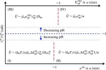
Here we present a detailed theoretical study which demonstrates however that electrokinetic effects (Pagonabarraga, Rotenberg & Frenkel Reference Pagonabarraga, Rotenberg and Frenkel2010) can also play a role in the motion of metallic-insulator spherical Janus particles expanding on our previous analyses briefly presented in Ebbens et al. (Reference Ebbens, Gregory, Dunderdale, Howse, Ibrahim, Liverpool and Golestanian2014). We find that their motion is due to a combination of neutral and ionic-diffusiophoretic as well as electrophoretic effects whose interplay can be changed by varying the ionic properties of the fluid (see figure 8). This has great potential significance as the effect on the swimming behaviour, of solution properties such as temperature (Balasubramanian et al. Reference Balasubramanian, Kagan, Manesh, Calvo-Marzal, Flechsig and Wang2009), contaminants (Zhao et al. Reference Zhao, Sanchez, Schmidt and Pumera2013), pH and salt concentration are of critical importance to potential applications (Patra et al. Reference Patra, Sengupta, Duan, Zhang, Pavlick and Sen2013).
We consider a Janus polystyrene (insulating) spherical colloid of radius
 $a$
, half-coated by a platinum (conducting) shell. It is known that such colloids are active i.e. self-propel in hydrogen peroxide solution. This is due to gradients generated by the asymmetric decomposition of
 $\text{H}_{2}\text{O}_{2}$
on the Pt-coating and the interaction of the reactants and products with the sphere surface. In the rest of the paper we will call this process self-phoresis.
Generically, the catalytic decomposition of the hydrogen peroxide by the platinum catalyst is given by
 $$\begin{eqnarray}\text{Pt}+2\text{H}_{2}\text{O}_{2}\rightarrow \displaystyle \text{Intermediate-complexes}\rightarrow \text{Pt}+2\text{H}_{2}\text{O}+\text{O}_{2},\end{eqnarray}$$
however there is still some debate about the nature of the intermediate complexes Hall, Khudaish & Hart (Reference Hall, Khudaish and Hart1998, Reference Hall, Khudaish and Hart1999a ,Reference Hall, Khudaish and Hart b ), Katsounaros et al. (Reference Katsounaros, Schneider, Meier, Benedikt, Biedermann, Auer and Mayrhofer2012).
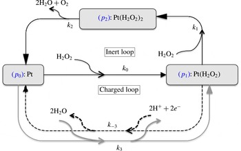
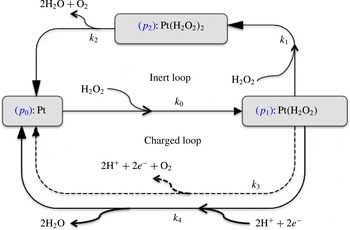
In this article, we outline a detailed calculation of the self-phoresis problem. Our approach is guided by the well-studied problem of a phoretic motion of a colloid in an externally applied concentration gradient or electric field. To model the effect of the non-equilibrium chemical reaction sketched above on the motion of the Janus particle, we study the concentration fields of all the species involved in the reaction. The half-coating of the colloid by catalyst is reflected by inhomogeneous reactive boundary conditions on its surface. The reaction involves the production of charged intermediates which can also lead to changes in the electric potential on the swimmer surface and hence the possibility of local electric fields. Our flexible calculation framework allows us to study a variety of different schemes for the reaction kinetics of the intermediate complexes. Using this we analyse in detail a scheme with both charged and uncharged pathways (see appendix A) whose results are consistent with all the behaviour observed in the recent experiments.
2 The model
A Janus sphere of radius
 $a$
has the catalytic reaction of hydrogen peroxide decomposition occurring on its Pt coated half. We choose, without loss of generality, that the normal to the plane splitting the hemispheres is aligned with the
 $z$
-axis (see figure 2). We propose a theoretical framework based on generally accepted properties of the reaction scheme for Pt catalysis of
 $\text{H}_{2}\text{O}_{2}$
degradation to water and
 $\text{O}_{2}$
(Hall et al.
Reference Hall, Khudaish and Hart1998, Reference Hall, Khudaish and Hart1999a
,Reference Hall, Khudaish and Hart
b
). A key feature of our analysis of self-propulsion is that it takes account of the existence of charged intermediates within the catalytic reaction scheme, namely protons and that the reaction rates varies with the Pt coating thickness (see figure 1).
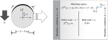
Schematic platinum–polystyrene swimmer and the domain decomposition of the phoretic problem.

The state of the system is therefore described by the local state of the Pt on the coated hemisphere, the electric potential,
 $\bar{\unicode[STIX]{x1D6F7}}(\bar{\boldsymbol{r}})$
, the fluid velocity,
 $\bar{\boldsymbol{v}}(\bar{\boldsymbol{r}})$
, the local concentrations,
 $\bar{c}_{hp}(\bar{\boldsymbol{r}}),\bar{c}_{o}(\bar{\boldsymbol{r}}),\bar{c}_{h}(\bar{\boldsymbol{r}})$
of
 $\text{H}_{2}\text{O}_{2}$
,
 $\text{O}_{2}$
and
 $\text{H}^{+}$
respectively, i.e. the various reactive species, and the local concentrations,
 $\bar{c}_{oh}(\bar{\boldsymbol{r}})$
,
 $\bar{c}_{s}(\bar{\boldsymbol{r}})$
of hydroxide and salt ions, respectively. The background concentrations (far from the Janus sphere) of the salt,
 $\text{H}_{2}\text{O}_{2}$
,
 $\text{H}^{+}$
and
 $\text{OH}^{-}$
are
 $c_{s}^{\infty },c_{hp}^{\infty },c_{h}^{\infty },c_{oh}^{\infty }$
respectively. Positions outside the Janus sphere (in the bulk) are represented by the vectors
 $\bar{\boldsymbol{r}}=(\bar{x},\bar{y},\bar{z})$
(in Cartesian coordinates) while positions on the surface are parametrized by the unit vectors
 $\hat{\boldsymbol{n}}=(\sin \unicode[STIX]{x1D703}\cos \unicode[STIX]{x1D719},\sin \unicode[STIX]{x1D703}\sin \unicode[STIX]{x1D719},\cos \unicode[STIX]{x1D703})$
. We note that the vector
 $\bar{\boldsymbol{r}}=(\bar{r},\unicode[STIX]{x1D703},\unicode[STIX]{x1D719})$
and
 $\hat{\boldsymbol{n}}=\hat{\boldsymbol{e}}_{\bar{r}}$
in spherical polar coordinates. Each of the neutral species interacts non-electrostatically with the surface of the swimmer via a fixed short-ranged potential energy
 $\bar{\unicode[STIX]{x1D6F9}}_{n}(\bar{\boldsymbol{r}})$
, that depends on the distance from the Janus sphere surface. The interaction range,
 $L_{eff}$
is taken to be the same for all neutral species.
2.1 Equations of motion
The relevant equations are Nernst–Planck equations (Probstein Reference Probstein2003) for the concentration of charged species,
 $\bar{c}_{q}$
,
 $$\begin{eqnarray}\displaystyle \unicode[STIX]{x2202}_{t}\bar{c}_{q}=-\bar{\unicode[STIX]{x1D735}}\boldsymbol{\cdot }\bar{\boldsymbol{J}}_{q};\quad \bar{\boldsymbol{J}}_{q}=-D_{q}\bar{\unicode[STIX]{x1D735}}\bar{c}_{q}+\bar{\boldsymbol{u}}_{q}\bar{c}_{q};\quad \bar{\boldsymbol{u}}_{q}=\bar{\boldsymbol{v}}-\frac{D_{q}z_{q}e}{k_{B}T}\bar{\unicode[STIX]{x1D735}}\bar{\unicode[STIX]{x1D6F7}}, & & \displaystyle\end{eqnarray}$$
drift-diffusion equations (Chandrasekhar Reference Chandrasekhar1943) for the neutral species,
 $\bar{c}_{n}$
,
 $$\begin{eqnarray}\displaystyle \unicode[STIX]{x2202}_{t}\bar{c}_{n}=-\bar{\unicode[STIX]{x1D735}}\boldsymbol{\cdot }\bar{\boldsymbol{J}}_{n};\quad \bar{\boldsymbol{J}}_{n}=-D_{n}\bar{\unicode[STIX]{x1D735}}\bar{c}_{n}+\bar{\boldsymbol{u}}_{n}\bar{c}_{n};\quad \bar{\boldsymbol{u}}_{n}=\bar{\boldsymbol{v}}-\frac{D_{n}}{k_{B}T}\bar{\unicode[STIX]{x1D735}}\bar{\unicode[STIX]{x1D6F9}}_{n}, & & \displaystyle\end{eqnarray}$$
Poisson’s equation (Jackson Reference Jackson1975) for the electric potential
 $$\begin{eqnarray}\displaystyle \bar{\unicode[STIX]{x1D6FB}}^{2}\bar{\unicode[STIX]{x1D6F7}}=-\mathop{\sum }_{q}\frac{z_{q}e\bar{c}_{q}}{\unicode[STIX]{x1D716}} & & \displaystyle\end{eqnarray}$$
and the incompressible Navier–Stokes equations (Lamb Reference Lamb1932) for the fluid velocity
 $$\begin{eqnarray}\displaystyle \left.\begin{array}{@{}c@{}}\displaystyle \unicode[STIX]{x1D70C}(\unicode[STIX]{x2202}_{t}\bar{\boldsymbol{v}}+\bar{\boldsymbol{v}}\boldsymbol{\cdot }\bar{\unicode[STIX]{x1D735}}\bar{\boldsymbol{v}})=\unicode[STIX]{x1D702}\bar{\unicode[STIX]{x1D6FB}}^{2}\bar{\boldsymbol{v}}-\bar{\unicode[STIX]{x1D735}}\bar{p}+\bar{\boldsymbol{f}}(\bar{\boldsymbol{r}});\quad \bar{\unicode[STIX]{x1D735}}\boldsymbol{\cdot }\bar{\boldsymbol{v}}=0,\\ \displaystyle \bar{\boldsymbol{f}}(\bar{\boldsymbol{r}})=\mathop{\sum }_{q}\unicode[STIX]{x1D6E4}_{q}\bar{c}_{q}(\bar{\boldsymbol{u}}_{q}-\bar{\boldsymbol{v}})+\mathop{\sum }_{n}\unicode[STIX]{x1D6E4}_{n}\bar{c}_{n}\left(\bar{\boldsymbol{u}}_{n}-\bar{\boldsymbol{v}}\right);\quad \unicode[STIX]{x1D6E4}_{q}=\frac{k_{B}T}{D_{q}},\quad \unicode[STIX]{x1D6E4}_{n}=\frac{k_{B}T}{D_{n}},\end{array}\right\} & & \displaystyle\end{eqnarray}$$
where
 $\bar{p}(\bar{\boldsymbol{r}})$
is the hydrostatic pressure at
 $\bar{\boldsymbol{r}}$
,
 $\unicode[STIX]{x1D702}$
is the viscosity,
 $k_{B}$
Boltzmann constant and
 $T$
temperature,
 $D_{i}$
is the diffusion coefficient of
 $i$
th solute and
 $z_{i}$
its valency if charged. These equations together with the inhomogeneous boundary conditions (BC) on the surface of the Janus sphere and as
 $\bar{r}\rightarrow \infty$
(see next section) define a boundary value problem whose approximate solution is the subject of this paper.
We consider the system in the steady state (time derivatives equal to zero), the dynamics of the fluid around the swimmer in the zero Reynolds number (
 $Re=0$
) limit of the Navier–Stokes equations for incompressible fluid flow. In this paper we restrict ourselves to zero Peclét number, equivalent to assuming that diffusion of the solutes occurs much faster than their convection by the flows generated by the Janus particle – very reasonable for the experimental systems we attempt to describe. Thus, the fluid velocity given by
 $\bar{\boldsymbol{v}}(\bar{\boldsymbol{r}})=\bar{v}_{r}\hat{\boldsymbol{e}}_{\bar{r}}+\bar{v}_{\unicode[STIX]{x1D703}}\hat{\boldsymbol{e}}_{\unicode[STIX]{x1D703}}$
obeys the Stokes equation, while the solute concentration fields
 $\bar{c}_{q},\bar{c}_{n}$
are governed by the steady-state drift-diffusion equations.
 $$\begin{eqnarray}\displaystyle & \displaystyle 0=\bar{\unicode[STIX]{x1D735}}\boldsymbol{\cdot }\bar{\boldsymbol{v}}, & \displaystyle\end{eqnarray}$$
 $$\begin{eqnarray}\displaystyle & \displaystyle \mathbf{0}=\unicode[STIX]{x1D735}\boldsymbol{\cdot }\bar{\unicode[STIX]{x1D72B}}+\bar{\boldsymbol{f}}=\unicode[STIX]{x1D702}\bar{\unicode[STIX]{x1D6FB}}^{2}\bar{\boldsymbol{v}}-\bar{\unicode[STIX]{x1D735}}\bar{p}-\mathop{\sum }_{i\in \,ions}ez_{i}\bar{c}_{i}\bar{\unicode[STIX]{x1D735}}\bar{\unicode[STIX]{x1D6F7}}-\mathop{\sum }_{j\in \,non\text{-}ions}\bar{c}_{j}\bar{\unicode[STIX]{x1D735}}\bar{\unicode[STIX]{x1D6F9}}_{j}, & \displaystyle\end{eqnarray}$$
 $$\begin{eqnarray}\displaystyle & \displaystyle 0=-\bar{\unicode[STIX]{x1D735}}\boldsymbol{\cdot }\bar{\boldsymbol{J}}_{q};\quad \bar{\boldsymbol{J}}_{q}=-D_{q}\bar{\unicode[STIX]{x1D735}}\bar{c}_{q}-\frac{D_{q}z_{q}e\bar{c}_{q}}{k_{B}T}\bar{\unicode[STIX]{x1D735}}\bar{\unicode[STIX]{x1D6F7}};\quad q\in \text{ions}, & \displaystyle\end{eqnarray}$$
 $$\begin{eqnarray}\displaystyle & \displaystyle 0=-\bar{\unicode[STIX]{x1D735}}\boldsymbol{\cdot }\bar{\boldsymbol{J}}_{n};\quad \bar{\boldsymbol{J}}_{n}=-D_{n}\bar{\unicode[STIX]{x1D735}}\bar{c}_{n}-\frac{D_{n}\bar{c}_{n}}{k_{B}T}\bar{\unicode[STIX]{x1D735}}\bar{\unicode[STIX]{x1D6F9}}_{n};\quad n\in \text{non-ions}, & \displaystyle\end{eqnarray}$$
where we have defined
 $\bar{\unicode[STIX]{x1D72B}}(\bar{\boldsymbol{r}})=\unicode[STIX]{x1D702}(\unicode[STIX]{x1D735}\boldsymbol{v}+\unicode[STIX]{x1D735}\boldsymbol{v}^{\text{T}})-p\unicode[STIX]{x1D739}$
, the local hydrodynamic stress tensor.
2.2 Boundary conditions
The hydroxide and the salt ions are not involved directly in the catalytic decomposition of the fuel (1.1) so we impose zero flux boundary conditions for their concentrations on the surface of the Janus particle,
 $$\begin{eqnarray}\hat{\boldsymbol{n}}\boldsymbol{\cdot }\bar{\boldsymbol{J}}_{oh}|_{\bar{r}=a}=0=\hat{\boldsymbol{n}}\boldsymbol{\cdot }\bar{\boldsymbol{J}}_{s,\pm }|_{\bar{r}=a},\end{eqnarray}$$
where the unit vector,
 $\hat{\boldsymbol{n}}=(\sin \unicode[STIX]{x1D703}\cos \unicode[STIX]{x1D719},\sin \unicode[STIX]{x1D703}\sin \unicode[STIX]{x1D719},\cos \unicode[STIX]{x1D703})=\hat{\boldsymbol{e}}_{r}$
in spherical polar coordinates. We define a catalyst coverage function,
 $K(\cos \unicode[STIX]{x1D703})$
which is
 $1$
on the platinum hemisphere and zero on the polystyrene hemisphere,
 $$\begin{eqnarray}K(\cos \unicode[STIX]{x1D703})=\left\{\begin{array}{@{}ll@{}}1,\quad & 0\leqslant \cos \unicode[STIX]{x1D703}\leqslant 1\\ 0,\quad & -1\leqslant \cos \unicode[STIX]{x1D703}<0.\end{array}\right.\end{eqnarray}$$
The presence of protons as intermediates of the fuel decomposition reaction (1.1) and the variation of the reaction rates across the Pt-coated hemisphere leads to non-zero flux boundary conditions for the proton concentration on the surface of the Janus sphere
 $$\begin{eqnarray}\displaystyle \hat{\boldsymbol{n}}\boldsymbol{\cdot }\bar{\boldsymbol{J}}_{h}|_{\bar{r}=a}=\bar{{\mathcal{J}}}_{h}(\unicode[STIX]{x1D703})K(\cos \unicode[STIX]{x1D703}), & & \displaystyle\end{eqnarray}$$
where the proton current,
 $\bar{{\mathcal{J}}}_{h}$
, varies with
 $\unicode[STIX]{x1D703}$
(position along the Pt-coated hemisphere). The specific form of the proton current
 $\bar{{\mathcal{J}}}_{h}$
will depend on the details of the reaction kinetics (see § 2.4 and appendix A). However, we note that
 $\bar{{\mathcal{J}}}_{h}>0$
implies a chemical reaction producing protons while
 $\bar{{\mathcal{J}}}_{h}<0$
implies a proton sink.
The fuel decomposition reaction involves the neutral species,
 $\text{H}_{2}\text{O}_{2}$
and
 $\text{O}_{2}$
giving rise to non-zero flux boundary conditions for their concentrations on the Janus particle surface,
 $$\begin{eqnarray}\displaystyle & \displaystyle \hat{\boldsymbol{n}}\boldsymbol{\cdot }\bar{\boldsymbol{J}}_{o}|_{\bar{r}=a}=\bar{{\mathcal{J}}}_{o}(\unicode[STIX]{x1D703})K(\cos \unicode[STIX]{x1D703}), & \displaystyle\end{eqnarray}$$
 $$\begin{eqnarray}\displaystyle & \displaystyle \hat{\boldsymbol{n}}\boldsymbol{\cdot }\bar{\boldsymbol{J}}_{hp}|_{\bar{r}=a}=\bar{{\mathcal{J}}}_{hp}(\unicode[STIX]{x1D703})K(\cos \unicode[STIX]{x1D703}), & \displaystyle\end{eqnarray}$$
where
 $\bar{{\mathcal{J}}}_{hp}(\unicode[STIX]{x1D703})<0$
indicates
 $\text{H}_{2}\text{O}_{2}$
decomposition while
 $\bar{{\mathcal{J}}}_{o}(\unicode[STIX]{x1D703})>0$
indicates production of the
 $\text{O}_{2}$
. Because of the variations in thickness of the Pt-coating, both
 $\bar{{\mathcal{J}}}_{hp}(\unicode[STIX]{x1D703}),\bar{{\mathcal{J}}}_{o}(\unicode[STIX]{x1D703})$
, defined in appendix A, are functions of position along the Pt-coated hemisphere.
All the concentrations,
 $\bar{c_{i}}(\bar{\boldsymbol{r}})$
, decay to their background values,
 $\bar{c}_{i}^{\infty }$
as
 $\bar{r}\rightarrow \infty$
.
We have Dirichlet boundary conditions for the electric potential on the particle surface
 $$\begin{eqnarray}\bar{\unicode[STIX]{x1D6F7}}(\bar{r}=a)=\bar{\unicode[STIX]{x1D711}}_{s}(\unicode[STIX]{x1D703}),\end{eqnarray}$$
where
 $\bar{\unicode[STIX]{x1D711}}_{s}$
is a possibly varying function over the swimmer surface. The potential,
 $\bar{\unicode[STIX]{x1D711}}_{s}$
will in general be pH dependent and will also depend on the particular reaction scheme of catalytic fuel decomposition. For our analysis, it is sufficient to know the average value
 $\left\langle \bar{\unicode[STIX]{x1D711}}_{s}\right\rangle =(1/2\unicode[STIX]{x03C0})\int \text{d}\cos \unicode[STIX]{x1D703}\,\bar{\unicode[STIX]{x1D711}}_{s}(\unicode[STIX]{x1D703})$
and in the following we take
 $\bar{\unicode[STIX]{x1D711}}_{s}\equiv \left\langle \bar{\unicode[STIX]{x1D711}}_{s}\right\rangle$
. The potential
 $\bar{\unicode[STIX]{x1D711}}_{s}$
can be related to the swimmer surface charge by double-layer models (Russel, Saville & Schowalter Reference Russel, Saville and Schowalter1992).
The boundary conditions for the fluid velocity field are
 $$\begin{eqnarray}\bar{\boldsymbol{v}}|_{\bar{r}=a}=\bar{\boldsymbol{U}}+\bar{\unicode[STIX]{x1D734}}\times \bar{\boldsymbol{r}};\quad \bar{\boldsymbol{v}}(\bar{r}\rightarrow \infty )=\mathbf{0},\end{eqnarray}$$
where
 $\bar{\boldsymbol{U}},\bar{\unicode[STIX]{x1D734}}$
are respectively the total linear and angular propulsion velocities of the swimmer. These are unknown and their calculation is the goal of this paper.
2.3 Constraints
(Quasi-steady state condition) As we study the system in a quasi-steady state, this requires that the average proton current on the swimmer surface vanishes,
 $$\begin{eqnarray}\oint _{\bar{r}=a}\bar{{\mathcal{J}}}_{h}(\unicode[STIX]{x1D703})K(\cos \unicode[STIX]{x1D703})\sin \unicode[STIX]{x1D703}\,\text{d}\unicode[STIX]{x1D703}=0,\end{eqnarray}$$
and note that this also guarantees conservation of the surface charge (Moran & Posner Reference Moran and Posner2011).
(Swimming conditions) We consider a freely swimming Janus particle with no external load on the colloid which requires that there is zero total force and torque on the swimmer:
 $$\begin{eqnarray}\displaystyle & \displaystyle \bar{\boldsymbol{F}}=\oint _{\bar{r}=a}\bar{\unicode[STIX]{x1D72B}}\boldsymbol{\cdot }\hat{\boldsymbol{n}}\,\text{d}{\mathcal{S}}_{p}+\int \bar{\boldsymbol{f}}\,\text{d}{\mathcal{V}}_{p}=\mathbf{0}, & \displaystyle\end{eqnarray}$$
 $$\begin{eqnarray}\displaystyle & \displaystyle \bar{\boldsymbol{T}}=\oint _{\bar{r}=a}\bar{\boldsymbol{r}}\times \left(\bar{\unicode[STIX]{x1D72B}}\boldsymbol{\cdot }\hat{\boldsymbol{n}}\right)\,\text{d}{\mathcal{S}}_{p}+\int \bar{\boldsymbol{r}}\times \bar{\boldsymbol{f}}\,\text{d}{\mathcal{V}}_{p}=\mathbf{0}, & \displaystyle\end{eqnarray}$$
where
 $\text{d}{\mathcal{S}}_{p}$
(
 $\text{d}{\mathcal{V}}_{p}$
) is the differential surface (volume) element. These two conditions uniquely determine both propulsion velocities
 $(\bar{\boldsymbol{U}},\bar{\unicode[STIX]{x1D734}})$
(Anderson Reference Anderson1989).
The linearity of the Stokes equation and the limit of vanishing Peclét number, mean that we can divide the linear and angular velocities into non-electric, i.e. neutral diffusiophoretic, (due to the terms on the right-hand side of (2.6) depending on the
 $\bar{\unicode[STIX]{x1D6F9}}_{j}$
), and electric, i.e. ionic-diffusiophoretic and electrophoretic, contributions (due to the terms on the right-hand side of (2.6) depending on
 $\bar{\unicode[STIX]{x1D6F7}}$
), which can each be calculated separately,
 $$\begin{eqnarray}\displaystyle & \displaystyle \bar{\boldsymbol{U}}=\bar{\boldsymbol{U}}^{e}+\bar{\boldsymbol{U}}^{d}, & \displaystyle\end{eqnarray}$$
 $$\begin{eqnarray}\displaystyle & \displaystyle \bar{\unicode[STIX]{x1D734}}=\bar{\unicode[STIX]{x1D734}}^{e}+\bar{\unicode[STIX]{x1D734}}^{d}, & \displaystyle\end{eqnarray}$$
where (
 $\bar{\boldsymbol{U}}^{e},\bar{\unicode[STIX]{x1D734}}^{e}$
) are electric and (
 $\bar{\boldsymbol{U}}^{d},\bar{\unicode[STIX]{x1D734}}^{d}$
) are non-electric. We expect (and indeed find) that the neutral-diffusiophoretic contribution to the propulsion is much smaller than the electrophoretic contribution. While we will later briefly outline the calculation of the neutral-diffusiophoretic contribution to the propulsion velocity in § 3.2, in this article we will focus on the electrophoretic and ionic-diffusiophoretic contributions. Detailed calculations of the neutral-diffusiophoretic contribution can be found in the literature (Anderson, Lowell & Prieve Reference Anderson, Lowell and Prieve1982; Golestanian et al.
Reference Golestanian, Liverpool and Ajdari2005, Reference Golestanian, Liverpool and Ajdari2007; Michelin & Lauga Reference Michelin and Lauga2014).
Due to the axisymmetry of the swimmer and the constraint of zero torque (2.18), the angular velocity
 $(\bar{\unicode[STIX]{x1D734}})$
vanishes identically
 $(\bar{\unicode[STIX]{x1D734}}^{e}=\mathbf{0},\bar{\unicode[STIX]{x1D734}}^{d}=\mathbf{0})$
. Therefore in the following we will only consider the swimmer velocity
 $\bar{\boldsymbol{U}}$
.
2.4 Dependence of reaction rate constants on Pt-coating thickness
The cornerstone of our analysis in this paper is the identification of the fact that the reaction rate of
 $\text{H}_{2}\text{O}_{2}$
decomposition depends on the Pt-coating thickness (Ebbens et al.
Reference Ebbens, Gregory, Dunderdale, Howse, Ibrahim, Liverpool and Golestanian2014). A further observation is the well-known presence of additional chemical pathways in the decomposition which involve charged intermediates, in particular protons, (Hall et al.
Reference Hall, Khudaish and Hart1998, Reference Hall, Khudaish and Hart1999a
,Reference Hall, Khudaish and Hart
b
). These charged intermediates, in conjunction with the variation of Pt-coating thickness, allow an electric current to be established in the Pt shell due to varying decomposition rates of the hydrogen peroxide on different parts of the shell. We approximate for simplicity that this thickness variation is linear in
 $\cos \unicode[STIX]{x1D703}$
, with a peak at the pole and the minimum at the equator,
 $$\begin{eqnarray}k_{i}(\unicode[STIX]{x1D703})=k_{i}^{(0)}+\mathop{\sum }_{l}k_{i}^{(l)}P_{l}\left(\cos \unicode[STIX]{x1D703}\right)\simeq k_{i}^{(0)}+k_{i}^{(1)}\cos \unicode[STIX]{x1D703},\end{eqnarray}$$
where
 $k_{i}(\unicode[STIX]{x1D703})$
is the reaction rate ‘constant’ for the
 $i$
th reaction step in reaction (1.1) above and
 $P_{n}(x)$
is the Legendre polynomial of order
 $n$
. The Legendre moments
 $k_{i}^{(l)}=(l+1/2)\int _{-1}^{1}k_{i}(\unicode[STIX]{x1D703})P_{l}(\cos \unicode[STIX]{x1D703})\,\text{d}\cos \unicode[STIX]{x1D703}$
. We assume weak variation (
 $k_{i}^{(1)}\ll k_{i}^{(0)}$
) allowing us to work perturbatively in the variation. As long as there is a competition between a neutral pathway and a pathway involving charged intermediates, conservation of charge in the steady state requires that the varying reaction rates across the Pt-coating lead to establishment of electric currents in the Pt shell. This is described in detail for a particular reaction scheme involving protons in appendix A, however the qualitative features of our results do not depend on the details of the scheme.
3 Analysis
Guided by current experiments, we analyse the coupled problem of the concentrations, electrostatic potential and fluid flow by considering situations in which the length scale of the interactions (Debye screening length,
 $\unicode[STIX]{x1D705}^{-1}$
for charged species and effective interaction range
 $L_{eff}$
for the neutral species) is small compared to the size (radius
 $=a$
) of the swimmer. We verify a posteriori that this is indeed the case. The effective diffusiophoretic interaction range
 $L_{eff}$
for all the neutral solutes is defined as
 $L_{eff}^{2}=(\unicode[STIX]{x1D702}/k_{B}T)\bar{\unicode[STIX]{x1D707}}_{d}^{\ddagger }$
, where
 $\bar{\unicode[STIX]{x1D707}}_{d}^{\ddagger }=(k_{B}T/\unicode[STIX]{x1D702})\int _{0}^{\infty }\unicode[STIX]{x1D70C}(1-e^{-\bar{\unicode[STIX]{x1D6F9}}/k_{B}T})\,\text{d}\unicode[STIX]{x1D70C}>0$
is the characteristic diffusiophoretic mobility of the Janus particle. Hence the problem can naturally be viewed as one with two very separate length scales with small parameters
 $\unicode[STIX]{x1D706}=1/(\unicode[STIX]{x1D705}a),\unicode[STIX]{x1D712}=L_{eff}/a$
for charged and neutral species respectively. A robust bound for comparison with experiment would be
 $\unicode[STIX]{x1D706}\leqslant 0.1$
. A useful approach to multi-scale problems with a small parameter multiplying the differential operator of highest order, is the decomposition of the domain of the solution into a boundary layer, where the fields vary on the small
 $O(\unicode[STIX]{x1D706})$
length scale (
 $O(\unicode[STIX]{x1D712})$
for the diffusiophoretic contribution) and an outer domain where the characteristic length scale is the size of the swimmer ‘
 $a$
’. To do this most efficiently, we group the dimensional quantities into useful dimensionless groups whose variation determines the behaviour of the system.
3.1 Self-electrophoresis and ionic self-diffusiophoresis
In this section, we describe detailed calculations of the electrophoretic and ionic-diffusiophoretic contributions to the swimming velocity which is the main focus of the paper.
3.1.1 Dimensionless equations
We non-dimensionalize the equations as follows. The position vector
 $\bar{\boldsymbol{r}}$
is measured in units of the swimmer size ‘
 $a$
’, concentrations
 $\bar{c}_{i}$
in units of the steady-state background values
 $c_{i}^{\infty }$
, electric potential
 $\bar{\unicode[STIX]{x1D6F7}}$
in terms of the thermal voltage
 $(e\unicode[STIX]{x1D6FD})^{-1}$
(with
 $\unicode[STIX]{x1D6FD}^{-1}=k_{B}T$
,
 $k_{B}$
Boltzmann constant and
 $T$
temperature), ionic solute fluxes,
 $\bar{\boldsymbol{J}}_{q}$
in terms of
 $D_{q}\sum _{i}|z_{i}|^{2}c_{i}^{\infty }/a$
, with
 $D_{i}$
the diffusion coefficient of
 $i$
th solute and
 $z_{i}$
its valency. The fluid flow velocity
 $\bar{\boldsymbol{v}}$
is rescaled by
 $\unicode[STIX]{x1D716}/(e^{2}\unicode[STIX]{x1D6FD}^{2}\unicode[STIX]{x1D702}a)$
, while the pressure
 $\bar{p}$
is rescaled by
 $\unicode[STIX]{x1D716}/(e^{2}\unicode[STIX]{x1D6FD}^{2}a^{2})$
. Hence we express dimensionless quantities (without overbar) in terms of the dimensional (with overbar):
 $\boldsymbol{r}=(x,y,z)=\bar{\boldsymbol{r}}/a,c_{i}=\bar{c}_{i}/c_{i}^{\infty },\unicode[STIX]{x1D6F7}=e\unicode[STIX]{x1D6FD}\bar{\unicode[STIX]{x1D6F7}},\boldsymbol{v}=\bar{\boldsymbol{v}}e^{2}\unicode[STIX]{x1D6FD}^{2}\unicode[STIX]{x1D702}a/\unicode[STIX]{x1D716},p=\bar{p}e^{2}\unicode[STIX]{x1D6FD}^{2}a/\unicode[STIX]{x1D716}$
.
It is useful for us to define the dimensionless deviations of the solute concentrations,
 $C_{i}(\boldsymbol{r})\equiv c_{i}(\boldsymbol{r})-1=(\bar{c}_{i}/c_{i}^{\infty })-1$
from their bulk values. Hence we obtain the following dimensionless equations of motion:
-
(i) The steady-state equations for concentration differences of the charged species; protons
 $C_{h}$
, hydroxide ions
$C_{oh}$
and the salt
$C_{s\pm }$
, (3.1a,b )where
$$\begin{eqnarray}\unicode[STIX]{x1D735}\boldsymbol{\cdot }\boldsymbol{J}_{i}=0;\quad \boldsymbol{J}_{i}=-\unicode[STIX]{x1D735}C_{i}-z_{i}(1+C_{i})\unicode[STIX]{x1D735}\unicode[STIX]{x1D6F7},\end{eqnarray}$$
$i\in \{h,oh,s\pm \}$
. We consider only monovalent salts
$|z_{i}|=1$
.
-
(ii) The dimensionless Poisson equation for the electric potential
$\unicode[STIX]{x1D6F7}(\boldsymbol{r})$
, (3.2)
$$\begin{eqnarray}-\unicode[STIX]{x1D706}^{2}\unicode[STIX]{x1D6FB}^{2}\unicode[STIX]{x1D6F7}=\mathop{\sum }_{i\in \{h,oh,s\pm \}}{\mathcal{Z}}_{i}C_{i}.\end{eqnarray}$$
-
(iii) The dimensionless Stokes equations for the fluid velocity
$\boldsymbol{v}(\boldsymbol{r})$
, (3.3)
$$\begin{eqnarray}\displaystyle & \displaystyle 0=\unicode[STIX]{x1D735}\boldsymbol{\cdot }\boldsymbol{v}, & \displaystyle\end{eqnarray}$$
(3.4)
$$\begin{eqnarray}\displaystyle & \displaystyle \mathbf{0}=\unicode[STIX]{x1D735}\boldsymbol{\cdot }\unicode[STIX]{x1D72E}=\unicode[STIX]{x1D6FB}^{2}\boldsymbol{v}-\unicode[STIX]{x1D735}p-\unicode[STIX]{x1D706}^{-2}\mathop{\sum }_{i\in \,ions}{\mathcal{Z}}_{i}C_{i}\unicode[STIX]{x1D735}\unicode[STIX]{x1D6F7}, & \displaystyle\end{eqnarray}$$


where the dimensionless parameters
 $\unicode[STIX]{x1D706}$
and
 ${\mathcal{Z}}_{i}$
are defined as
 $$\begin{eqnarray}\unicode[STIX]{x1D706}^{2}\equiv \left(\unicode[STIX]{x1D705}a\right)^{-2};\quad \unicode[STIX]{x1D705}^{-2}=\frac{\unicode[STIX]{x1D716}k_{B}T}{e^{2}\mathop{\sum }_{j}|z_{j}|^{2}c_{j}^{\infty }}=\frac{1}{4\unicode[STIX]{x03C0}l_{B}\mathop{\sum }_{j}|z_{j}|^{2}c_{j}^{\infty }};\quad {\mathcal{Z}}_{i}=\frac{z_{i}c_{i}^{\infty }}{\mathop{\sum }_{j}|z_{j}|^{2}c_{j}^{\infty }},\end{eqnarray}$$
where
 $\unicode[STIX]{x1D716}$
is the permittivity of the solvent and
 $e$
is the electronic charge.
 $\unicode[STIX]{x1D705}^{-1}$
is the Debye screening length and
 $l_{B}=e^{2}/4\unicode[STIX]{x03C0}\unicode[STIX]{x1D716}k_{B}T$
is the Bjerrum length (Russel et al.
Reference Russel, Saville and Schowalter1992). We note that the stress
 $\unicode[STIX]{x1D72E}$
is the sum of the hydrodynamic stress tensor and the Maxwell stress tensor due to the interactions of the charged species with each other and the colloid surface.
The zero total force condition which determines the propulsion velocity
 $\boldsymbol{U}^{e}$
becomes
 $$\begin{eqnarray}\boldsymbol{F}=\oint _{r=1}\unicode[STIX]{x1D72E}\boldsymbol{\cdot }\hat{\boldsymbol{n}}\sin \unicode[STIX]{x1D703}\,\text{d}\unicode[STIX]{x1D703}=\mathbf{0}.\end{eqnarray}$$
3.1.2 Dimensionless boundary conditions
For the electric potential on the swimmer surface,
 $$\begin{eqnarray}\unicode[STIX]{x1D6F7}(r=1)=\unicode[STIX]{x1D711}_{s},\end{eqnarray}$$
and decays to zero in the bulk far from the swimmer,
 $\unicode[STIX]{x1D6F7}(r\rightarrow \infty )=0$
.
For the flow field on the swimmer surface,
 $$\begin{eqnarray}\displaystyle \boldsymbol{v}|_{r=1}=\boldsymbol{U}^{e}, & & \displaystyle\end{eqnarray}$$
and
 $\boldsymbol{v}(r\rightarrow \infty )=\mathbf{0}$
far in the bulk, where
 $\boldsymbol{U}^{e}$
is the electric contribution to the propulsion velocity.
For the hydroxide and the salt concentrations, the zero flux boundary conditions due to the impermeability of the Janus particle surface,
 $$\begin{eqnarray}\hat{\boldsymbol{n}}\boldsymbol{\cdot }\boldsymbol{J}_{oh}|_{r=1}=0=\hat{\boldsymbol{n}}\boldsymbol{\cdot }\boldsymbol{J}_{s,\pm }|_{r=1}.\end{eqnarray}$$
For the proton concentration, the non-zero flux boundary condition,
 $$\begin{eqnarray}\hat{\boldsymbol{n}}\boldsymbol{\cdot }\boldsymbol{J}_{h}|_{r=1}={\mathcal{J}}_{h}(\unicode[STIX]{x1D703})K(\cos \unicode[STIX]{x1D703}).\end{eqnarray}$$
The essential mechanism which drives this process depends on the presence of a (i) varying proton flux (as a result of variation of Pt thickness) which (ii) averages to zero over the metallic hemisphere (due to charge conservation in the steady state). In the limit of small linear variation in the thickness, this leads to a proton flux of the general form
 $$\begin{eqnarray}{\mathcal{J}}_{h}(\unicode[STIX]{x1D703})=\unicode[STIX]{x1D6FE}^{(1)}\left(1-2\cos \unicode[STIX]{x1D703}\right)K(\cos \unicode[STIX]{x1D703})-\unicode[STIX]{x1D6FE}^{(0)}\unicode[STIX]{x1D6FF}\left(\unicode[STIX]{x1D6F7}+C_{h}\right)K(\cos \unicode[STIX]{x1D703}),\end{eqnarray}$$
where both
 $\unicode[STIX]{x1D6FE}^{(i)}\neq 0$
. We note that
 $\unicode[STIX]{x1D6FE}^{(1)}=0$
for a uniform thickness coating and
 $\unicode[STIX]{x1D6FF}(\unicode[STIX]{x1D6F7}+C_{h})=[(\unicode[STIX]{x1D6F7}+C_{h})-\int _{0}^{\unicode[STIX]{x03C0}}(\unicode[STIX]{x1D6F7}+C_{h})K(\cos \unicode[STIX]{x1D703})\sin \unicode[STIX]{x1D703}\,\text{d}\unicode[STIX]{x1D703}]$
is the deviation of the local electric field and proton concentration from their surface average.
 $\unicode[STIX]{x1D6FE}^{(0)}$
is a measure of the scale of typical production and consumption of protons across the metallic hemisphere. Since both terms on the right-hand side of (3.11) integrated over the surface give zero, the flux,
 ${\mathcal{J}}_{h}$
automatically satisfies the steady-state requirement (2.16) and hence the conservation of total charge on the swimmer surface.
Systems which possess both properties above, with both
 $\unicode[STIX]{x1D6FE}^{(i)}>0$
, will show all the qualitative behaviours described in this article, however their values will depend on the specific details of the chemical reaction scheme. A specific reaction scheme described in detail in appendix A gives:
 $$\begin{eqnarray}\unicode[STIX]{x1D6FE}^{(0)}=\frac{k_{eff}^{(h)}c_{hp}^{\infty }a}{D_{h}\mathop{\sum }_{i}c_{i}^{\infty }};\quad \unicode[STIX]{x1D6FE}^{(1)}=\frac{\unicode[STIX]{x0394}k_{eff}^{(h)}c_{hp}^{\infty }a}{D_{h}\mathop{\sum }_{i}c_{i}^{\infty }},\end{eqnarray}$$
where
 $k_{eff}^{(h)}>0$
is the typical scale of the average proton consumption and production while
 $\unicode[STIX]{x0394}k_{eff}^{(h)}>0$
is the scale of the difference between the rates at the pole and equator (see appendix A for their derivation from reaction kinetics).
We note that the conservation of protons also requires a relationship between the pH of the solution and the potential on the surface of the Janus particle, which depends on the reaction kinetics (see appendix A);
 $$\begin{eqnarray}\displaystyle \unicode[STIX]{x1D711}_{s}=\unicode[STIX]{x1D711}_{s}(c_{h}^{\infty }), & & \displaystyle\end{eqnarray}$$
leading to an estimate of the average swimmer surface charge
 $(\unicode[STIX]{x1D70E}_{0}(c_{h}^{\infty }))$
using the Gouy–Chapman model (Russel et al.
Reference Russel, Saville and Schowalter1992) of the interfacial double layer
 $$\begin{eqnarray}\unicode[STIX]{x1D70E}_{0}(c_{h}^{\infty })=\frac{e\unicode[STIX]{x1D705}}{2\unicode[STIX]{x03C0}l_{B}}\sinh \left(\frac{\unicode[STIX]{x1D711}_{s}}{2}\right),\end{eqnarray}$$
where
 $l_{B}=e^{2}/4\unicode[STIX]{x03C0}\unicode[STIX]{x1D716}k_{B}T$
is the Bjerrum length, with
 $\unicode[STIX]{x1D716}$
the solution permittivity.
In this electrostatic problem, the inner boundary layer (double layer) fields,
 $H(\boldsymbol{r})\in \{c_{i}(\boldsymbol{r}),\boldsymbol{v}(\boldsymbol{r}),\unicode[STIX]{x1D731}(\boldsymbol{r})\}$
are expanded as
 $$\begin{eqnarray}\displaystyle H(r,\unicode[STIX]{x1D703})=\mathop{\sum }_{n}\unicode[STIX]{x1D706}^{n}{\mathcal{H}}^{(n)}\left(\unicode[STIX]{x1D70C},\unicode[STIX]{x1D703}\right)\!;\quad \unicode[STIX]{x1D70C}=\frac{r-1}{\unicode[STIX]{x1D706}}, & & \displaystyle\end{eqnarray}$$
while the outer fields,
 $H(\boldsymbol{r})\in \{c_{i}(\boldsymbol{r}),\boldsymbol{v}(\boldsymbol{r}),\unicode[STIX]{x1D731}(\boldsymbol{r})\}$
are expanded as
 $$\begin{eqnarray}H(r,\unicode[STIX]{x1D703})=H^{(0)}(r,\unicode[STIX]{x1D703})+\mathop{\sum }_{n=1}^{\infty }\unicode[STIX]{x1D706}^{n}H^{(n)}(r,\unicode[STIX]{x1D703}),\end{eqnarray}$$
where
 $r$
is the bulk-scale coordinate. Similar expansions will apply for the self-diffusiophoretic problem, with
 $\unicode[STIX]{x1D706}$
replaced by
 $\unicode[STIX]{x1D712}$
.
The essence of the matched asymptotic method involves obtaining asymptotic expansions of the solutions of the equations in the limit
 $\unicode[STIX]{x1D706}\rightarrow 0$
for both the inner and outer fields and matching the results in the intermediate region:
 $$\begin{eqnarray}\lim _{\unicode[STIX]{x1D706}\rightarrow 0;\unicode[STIX]{x1D70C}\rightarrow \infty }\{{\mathcal{H}}_{i}^{(0)}\}\left(\unicode[STIX]{x1D70C},\unicode[STIX]{x1D703}\right)=\lim _{r\rightarrow 1;\unicode[STIX]{x1D706}\rightarrow 0}\{H_{i}^{(0)}\}(r,\unicode[STIX]{x1D703})=\{H_{i}\}(1,\unicode[STIX]{x1D703}).\end{eqnarray}$$
In the next section, we will proceed to solve the outer problem in the limit of
 $\unicode[STIX]{x1D706}=(\unicode[STIX]{x1D705}a)^{-1}\rightarrow 0$
, i.e. thin double-layer limit where the swimmer radius
 $a$
is much larger than the Debye-layer thickness
 $\unicode[STIX]{x1D705}^{-1}$
. The details of the inner (Debye-layer) calculations (Prieve et al.
Reference Prieve, Anderson, Ebel and Lowell1984; Yariv Reference Yariv2011) can be found in the appendix B (see figure 3).
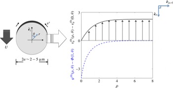
Profiles of flow and electric field within the (inner) Debye layer with
 $C_{s}^{\ast }=\unicode[STIX]{x2202}C_{s}^{\ast }/\unicode[STIX]{x2202}\unicode[STIX]{x1D703}=\unicode[STIX]{x2202}\unicode[STIX]{x1D6F7}/\unicode[STIX]{x2202}\unicode[STIX]{x1D703}=1$
(see appendix B).

3.1.3 Outer concentration and electric fields
In the bulk, the fields vary over length scales comparable to the swimmer size, with
 $O(1)$
leading-order fields, and are expanded as
 $$\begin{eqnarray}H(r,\unicode[STIX]{x1D703})=H^{(0)}(r,\unicode[STIX]{x1D703})+\unicode[STIX]{x1D706}H^{(1)}(r,\unicode[STIX]{x1D703})+\cdots \,.\end{eqnarray}$$
We drop the
 $^{(0)}$
superscript in the following as we will consider only the leading-order terms
 $C^{(0)},\unicode[STIX]{x1D6F7}^{(0)},v_{i}^{(0)},p^{(0)}$
, in the expansions for the fields.
The leading-order solute concentrations and electric potential outside the Debye layer obey the equations
 $$\begin{eqnarray}\displaystyle & \displaystyle \mathop{\sum }_{i\in \{h,oh,s\pm \}}{\mathcal{Z}}_{i}C_{i}=0, & \displaystyle\end{eqnarray}$$
 $$\begin{eqnarray}\displaystyle & \displaystyle \unicode[STIX]{x1D735}\boldsymbol{\cdot }\left[\unicode[STIX]{x1D735}C_{i}+z_{i}(1+C_{i})\unicode[STIX]{x1D735}\unicode[STIX]{x1D6F7}\right]=0, & \displaystyle\end{eqnarray}$$
where
 ${\mathcal{Z}}_{i}$
is defined in (3.5). It is useful for the rest of our analysis to treat all the ionic solutes together. Combining the two equations (3.19) and (3.20), we obtain,
 $$\begin{eqnarray}\displaystyle & \displaystyle \unicode[STIX]{x1D6FB}^{2}C^{\ast }=0, & \displaystyle\end{eqnarray}$$
 $$\begin{eqnarray}\displaystyle & \displaystyle \unicode[STIX]{x1D735}\boldsymbol{\cdot }\left(C^{\ast }\unicode[STIX]{x1D735}\unicode[STIX]{x1D6F7}\right)=0, & \displaystyle\end{eqnarray}$$
where we have defined the sum of the deviations of concentration of all of the ionic solutes and its value at
 $r=1$
.
 $$\begin{eqnarray}\displaystyle & \displaystyle C^{\ast }(r,\unicode[STIX]{x1D703})=2\mathop{\sum }_{i\in \{h,s+\}}{\mathcal{Z}}_{i}\left(1+C_{i}(r,\unicode[STIX]{x1D703})\right)\!; & \displaystyle\end{eqnarray}$$
 $$\begin{eqnarray}\displaystyle & \displaystyle C_{s}^{\ast }(\unicode[STIX]{x1D703})\equiv C^{\ast }(r=1,\unicode[STIX]{x1D703}). & \displaystyle\end{eqnarray}$$
The boundary conditions for
 $\unicode[STIX]{x1D6F7}$
and
 $C^{\ast }$
are obtained by matching to the inner solutions (see appendix B), giving
 $$\begin{eqnarray}\displaystyle & \displaystyle -\hat{\boldsymbol{n}}\boldsymbol{\cdot }\unicode[STIX]{x1D735}C^{\ast }|_{r=1}=\unicode[STIX]{x1D6FE}^{(1)}\left(1-2\cos \unicode[STIX]{x1D703}\right)K(\cos \unicode[STIX]{x1D703})-\unicode[STIX]{x1D6FE}^{(0)}\unicode[STIX]{x1D6FF}(\unicode[STIX]{x1D6F7}+C_{h})K(\cos \unicode[STIX]{x1D703}), & \displaystyle\end{eqnarray}$$
 $$\begin{eqnarray}\displaystyle & \displaystyle -\hat{\boldsymbol{n}}\boldsymbol{\cdot }\left(C^{\ast }\unicode[STIX]{x1D735}\unicode[STIX]{x1D6F7}\right|_{r=1}=\unicode[STIX]{x1D6FE}^{(1)}\left(1-2\cos \unicode[STIX]{x1D703}\right)K(\cos \unicode[STIX]{x1D703})-\unicode[STIX]{x1D6FE}^{(0)}\unicode[STIX]{x1D6FF}\left(\unicode[STIX]{x1D6F7}+C_{h}\right)K(\cos \unicode[STIX]{x1D703}), & \displaystyle\end{eqnarray}$$
from equations (3.10) and (3.11).
The fluid velocity field in the outer region obeys the equation
 $$\begin{eqnarray}\displaystyle \unicode[STIX]{x1D6FB}^{2}\boldsymbol{v}-\unicode[STIX]{x1D735}p+\unicode[STIX]{x1D6FB}^{2}\unicode[STIX]{x1D6F7}\unicode[STIX]{x1D735}\unicode[STIX]{x1D6F7}=\mathbf{0}, & & \displaystyle\end{eqnarray}$$
with the slip boundary condition (Prieve et al. Reference Prieve, Anderson, Ebel and Lowell1984)
 $$\begin{eqnarray}\displaystyle \boldsymbol{v}(1,\unicode[STIX]{x1D703})=\boldsymbol{U}^{e}+\left[\unicode[STIX]{x1D701}(\unicode[STIX]{x1D703})\frac{\unicode[STIX]{x2202}\unicode[STIX]{x1D6F7}}{\unicode[STIX]{x2202}\unicode[STIX]{x1D703}}+4\ln \cosh \left(\frac{\unicode[STIX]{x1D701}(\unicode[STIX]{x1D703})}{4}\right)\frac{\unicode[STIX]{x2202}\ln C_{s}^{\ast }}{\unicode[STIX]{x2202}\unicode[STIX]{x1D703}}\right]\hat{\boldsymbol{e}}_{\unicode[STIX]{x1D703}}, & & \displaystyle\end{eqnarray}$$
and quiescent fluid far away from the swimmer,
 $\boldsymbol{v}\rightarrow \mathbf{0}$
as
 $r\rightarrow \infty$
. The slip boundary condition for
 $\boldsymbol{v}$
is obtained by matching to the inner solution (see appendix B).
3.1.4 Linear response and propulsion velocity
We note that with uniform coating,
 $k_{i}=k_{i}^{(0)}$
, which implies
 $\unicode[STIX]{x1D6FE}^{(1)}=0$
, the deviations of the electric potential and the ionic concentrations vanish (
 $\unicode[STIX]{x1D6F7}=0=C_{i}$
). The
 $\unicode[STIX]{x1D701}$
potential for this trivial solution is
 $$\begin{eqnarray}\unicode[STIX]{x1D701}_{0}:=\unicode[STIX]{x1D701}=\unicode[STIX]{x1D711}_{s}.\end{eqnarray}$$
In addition, this implies the fluid velocity field vanishes
 $\boldsymbol{v}=\mathbf{0}$
, and hence the contribution of self-electrophoresis to the propulsion velocity vanishes
 $\boldsymbol{U}^{e}=\mathbf{0}$
. However, a varying thickness coating and the consequent non-zero
 $\unicode[STIX]{x1D6FE}^{(1)}$
, lead to a qualitatively different scenario. To explore this we perform an expansion to linear order in
 $\unicode[STIX]{x1D6FE}^{(1)}/\unicode[STIX]{x1D6FE}^{(0)}$
of the fields for the concentrations, fluid velocity, pressure and electric potential:
 $\{C_{i},\boldsymbol{v},p,\unicode[STIX]{x1D6F7}\}$
for
 $\unicode[STIX]{x1D6FE}^{(1)}\ll \unicode[STIX]{x1D6FE}^{(0)}$
, where
 $\unicode[STIX]{x1D6FE}^{(1)},\unicode[STIX]{x1D6FE}^{(0)}$
are defined in (3.12).
We first expand the deviations of the concentrations and the electric field as
 $$\begin{eqnarray}\displaystyle H=\unicode[STIX]{x1D6FE}^{(1)}H^{(\unicode[STIX]{x1D6FE})}+O((\unicode[STIX]{x1D6FE}^{(1)})^{2}), & & \displaystyle\end{eqnarray}$$
with
 $H\in \{C_{i},C^{\ast },\unicode[STIX]{x1D6F7}\}$
and keeping only linear terms. Substituting these perturbative fields into (3.21), (3.22), we find that at leading order,
 ${C^{\ast }}^{(\unicode[STIX]{x1D6FE})}$
decouples from the electric potential field
 $\unicode[STIX]{x1D6F7}^{(\unicode[STIX]{x1D6FE})}$
– with both obeying Laplace equations
 $$\begin{eqnarray}\displaystyle & \displaystyle \unicode[STIX]{x1D6FB}^{2}{C^{\ast }}^{(\unicode[STIX]{x1D6FE})}=0, & \displaystyle\end{eqnarray}$$
 $$\begin{eqnarray}\displaystyle & \displaystyle \unicode[STIX]{x1D6FB}^{2}\unicode[STIX]{x1D6F7}^{(\unicode[STIX]{x1D6FE})}=0, & \displaystyle\end{eqnarray}$$
and the boundary conditions, from the matching with the inner solution, at this order are
 $$\begin{eqnarray}\left.-\hat{\boldsymbol{n}}\boldsymbol{\cdot }\unicode[STIX]{x1D735}{C^{\ast }}^{(\unicode[STIX]{x1D6FE})}\right|_{r=1}=\left.-\hat{\boldsymbol{n}}\boldsymbol{\cdot }\unicode[STIX]{x1D735}\unicode[STIX]{x1D6F7}^{(\unicode[STIX]{x1D6FE})}\right|_{r=1}=\left(1-2x\right)K(x)-\unicode[STIX]{x1D6FE}^{(0)}\unicode[STIX]{x1D6FF}(\unicode[STIX]{x1D6F7}^{(\unicode[STIX]{x1D6FE})}+{C_{h}}^{(\unicode[STIX]{x1D6FE})})K(x),\end{eqnarray}$$
where
 $x=\cos \unicode[STIX]{x1D703}$
,
 $\unicode[STIX]{x1D6FF}(\unicode[STIX]{x1D6F7}^{(\unicode[STIX]{x1D6FE})}+{C_{h}}^{(\unicode[STIX]{x1D6FE})})=[(\unicode[STIX]{x1D6F7}^{(\unicode[STIX]{x1D6FE})}+{C_{h}}^{(\unicode[STIX]{x1D6FE})})-\int _{0}^{1}(\unicode[STIX]{x1D6F7}^{(\unicode[STIX]{x1D6FE})}+{C_{h}}^{(\unicode[STIX]{x1D6FE})})\,\text{d}x]$
.
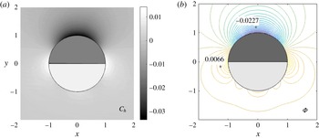
(a) Proton concentration deviation from the uniform background profile and (b) associated electric potential difference contours (both plots with
 $\text{pH}=5.5$
for 10 %
 $\text{H}_{2}\text{O}_{2}$
without salt and the system parameters in table 1). The equipotential contours
 $0.0066$
and
 $-0.0227$
(in units of the thermal voltage
 $(k_{B}T/e)\approx 25$
mV) are shown to indicate the electric pole–equator polarity. In both panels, the upper (dark) hemisphere is the platinum cap.

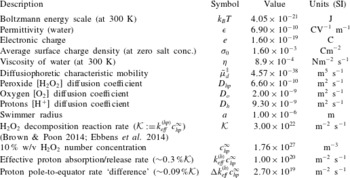
System parameters.

Now, the Laplace equations above for
 ${C^{\ast }}^{(\unicode[STIX]{x1D6FE})},\unicode[STIX]{x1D6F7}^{(\unicode[STIX]{x1D6FE})}$
in conjunction with the electroneutrality condition (3.19) imply (see figure 4)
 $$\begin{eqnarray}\unicode[STIX]{x1D6F7}^{(\unicode[STIX]{x1D6FE})}(r,\unicode[STIX]{x1D703})={C_{h}}^{(\unicode[STIX]{x1D6FE})}(r,\unicode[STIX]{x1D703})={C^{\ast }}^{(\unicode[STIX]{x1D6FE})}(r,\unicode[STIX]{x1D703})-1=\mathop{\sum }_{l=0}^{\infty }A_{l}r^{-(l+1)}P_{l}(\cos \unicode[STIX]{x1D703}),\end{eqnarray}$$
where
 $P_{l}(\cos \unicode[STIX]{x1D703})$
are the Legendre polynomials. The unknown coefficients
 $A_{l}$
are determined by the boundary conditions in (3.33) above.
Finally, the coefficients
 $A_{l}$
are obtained as a self-consistent system of equations,
 $$\begin{eqnarray}\mathop{\sum }_{l=0}^{\infty }A_{l}(l+1)P_{l}(x)=(1-2x)K(x)-2\unicode[STIX]{x1D6FE}^{(0)}\mathop{\sum }_{l=0}^{\infty }A_{l}\left(P_{l}\left(x\right)-\int _{0}^{1}P_{l}(x^{\prime })\,\text{d}x^{\prime }\right)K(x),\end{eqnarray}$$
where
 $x=\cos \unicode[STIX]{x1D703}$
.
Using the orthogonality of the Legendre polynomials, we obtain a linear system of equations for the coefficients
 $A_{l}$
,
 $$\begin{eqnarray}\left(\begin{array}{@{}cccccc@{}}1 & 0 & 0 & \cdots \, & 0 & \cdots \\ 0 & M_{11} & M_{12} & \cdots \, & M_{1l} & \cdots \\ 0 & M_{21} & M_{22} & \cdots \, & M_{2l} & \cdots \\ \vdots & \vdots & \vdots & \ddots & \vdots & \ldots \\ 0 & M_{n1} & M_{n2} & \ldots & M_{nl} & \ldots \\ \vdots & \vdots & \vdots & \vdots & \vdots & \ddots \end{array}\right)\left(\begin{array}{@{}c@{}}A_{0}\\ A_{1}\\ A_{2}\\ \vdots \\ A_{l}\\ \vdots \end{array}\right)=\left(\begin{array}{@{}c@{}}0\\ \unicode[STIX]{x1D6EC}_{1}\\ \unicode[STIX]{x1D6EC}_{2}\\ \vdots \\ \unicode[STIX]{x1D6EC}_{n}\\ \vdots \end{array}\right)\end{eqnarray}$$
or more compactly
 $$\begin{eqnarray}\displaystyle \unicode[STIX]{x1D648}\boldsymbol{\cdot }\boldsymbol{A}=\unicode[STIX]{x1D726}, & & \displaystyle\end{eqnarray}$$
where
 $\boldsymbol{A}=(A_{0},\ldots ,A_{N},\ldots )$
, and the matrix
 $\unicode[STIX]{x1D648}$
and vector
 $\unicode[STIX]{x1D726}$
entries are given by
 $$\begin{eqnarray}\displaystyle & \displaystyle M_{nl}=\unicode[STIX]{x1D6FF}_{nl}+\unicode[STIX]{x1D6FE}^{(0)}\left(\frac{2n+1}{n+1}\right)\int _{0}^{1}P_{n}(x)\left(P_{l}(x)-\int _{0}^{1}P_{l}(x^{\prime })\,\text{d}x^{\prime }\right)\,\text{d}x, & \displaystyle\end{eqnarray}$$
 $$\begin{eqnarray}\displaystyle & \displaystyle \unicode[STIX]{x1D6EC}_{n}=\frac{1}{2}\left(\frac{2n+1}{n+1}\right)\int _{0}^{1}\left(1-2x\right)P_{n}(x)\,\text{d}x. & \displaystyle\end{eqnarray}$$
The infinite linear system of equations (3.36) above can be solved approximately by truncating the infinite system after a finite number of components, reducing the description to the first
 $N$
Legendre coefficients
 $A_{l}$
. The approximate (numerical) solution requires inversion of an
 $N\times N$
matrix
 $\unicode[STIX]{x1D648}$
(see figure 5). However, we can extract asymptotic regimes of this solution for
 $\unicode[STIX]{x1D6FE}^{(0)}\ll 1$
and
 $\unicode[STIX]{x1D6FE}^{(0)}\gg 1$
. Note that
 $\unicode[STIX]{x1D6FE}^{(1)}\ll \unicode[STIX]{x1D6FE}^{(0)}$
in both limits.
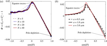
(a) The deviations of the surface electric potential,
 $\unicode[STIX]{x1D6F7}(1,\unicode[STIX]{x1D703})$
, and ionic concentrations,
 $C_{h}(1,\unicode[STIX]{x1D703}),C_{s}^{\ast }(1,\unicode[STIX]{x1D703})-1$
, from the uniform background values (for swimmer size
 $a=1.00~\unicode[STIX]{x03BC}\text{m}$
). We show the convergence of the solution as the number
 $N$
of the Legendre modes in (3.34) are increased, i.e.
 $\boldsymbol{A}=\{A_{0},\ldots ,A_{N-1},A_{N}\}$
. (b) The deviations of the surface potential and ionic concentration as a function of swimmer size
 $a$
(truncating at
 $N=40$
).

 $\unicode[STIX]{x1D6FE}^{(0)}\ll 1$
: In this regime,
 $A_{l}\sim \unicode[STIX]{x1D6EC}_{l}$
and
 $$\begin{eqnarray}A_{1}\sim -{\textstyle \frac{1}{8}}\end{eqnarray}$$
 $\unicode[STIX]{x1D6FE}^{(0)}\gg 1$
: In this regime,
 $$\begin{eqnarray}A_{1}\sim -\frac{\unicode[STIX]{x1D6FC}}{\unicode[STIX]{x1D6FE}^{(0)}},\end{eqnarray}$$
where
 $\unicode[STIX]{x1D6FC}$
is a positive constant whose value can be determined numerically. The asymptotes show that the perturbations of
 $C_{i}$
and
 $\unicode[STIX]{x1D6F7}$
decay to zero for large
 $\unicode[STIX]{x1D6FE}^{(0)}$
(proportional to swimmer size) – when the diffusion time becomes large compared to the reaction time.
In figure 5(a), the deviations of the proton concentration
 ${C_{h}}^{(\unicode[STIX]{x1D6FE})}(1,\unicode[STIX]{x1D703})$
and electric potential
 $\unicode[STIX]{x1D6F7}^{(\unicode[STIX]{x1D6FE})}(1,\unicode[STIX]{x1D703})$
on the surface from their bulk values are plotted showing the an excess at the equator and depletion at the pole. Increasing the number of Legendre polynomial modes (
 $N$
) improves the accuracy of the fields on the polystyrene hemisphere. The proton depletion (excess) at the pole (equator) is stronger for larger swimmer sizes (see figure 5
b).
The calculated coefficients
 $A_{l}$
above determine the slip velocity and we can now solve the Stokes flow problem. Hence, as above, we expand the velocity and pressure fields about the trivial solution
 $\boldsymbol{v}=\mathbf{0},p=p_{\infty }$
,
 $$\begin{eqnarray}\displaystyle & \displaystyle \boldsymbol{v}=\unicode[STIX]{x1D6FE}^{(1)}\boldsymbol{v}^{(\unicode[STIX]{x1D6FE})}+\cdots \,; & \displaystyle\end{eqnarray}$$
 $$\begin{eqnarray}\displaystyle & \displaystyle p-p_{\infty }=\unicode[STIX]{x1D6FE}^{(1)}p^{(\unicode[STIX]{x1D6FE})}+\cdots & \displaystyle\end{eqnarray}$$
and the propulsion velocity about the stationary colloid,
 $\boldsymbol{U}^{e}=\mathbf{0}$
 $$\begin{eqnarray}\displaystyle \boldsymbol{U}^{e}=\unicode[STIX]{x1D6FE}^{(1)}{\boldsymbol{U}^{e}}^{(\unicode[STIX]{x1D6FE})}+\cdots \,. & & \displaystyle\end{eqnarray}$$
Then, the Stokes equations become
 $$\begin{eqnarray}\displaystyle \unicode[STIX]{x1D6FB}^{2}\boldsymbol{v}^{(\unicode[STIX]{x1D6FE})}-\unicode[STIX]{x1D735}p^{(\unicode[STIX]{x1D6FE})}=\mathbf{0};\quad \unicode[STIX]{x1D735}\boldsymbol{\cdot }\boldsymbol{v}^{(\unicode[STIX]{x1D6FE})}=0, & & \displaystyle\end{eqnarray}$$
with the slip boundary condition from matching to the inner solution,
 $$\begin{eqnarray}\boldsymbol{v}^{(\unicode[STIX]{x1D6FE})}(1,\unicode[STIX]{x1D703})={\boldsymbol{U}^{e}}^{(\unicode[STIX]{x1D6FE})}+\unicode[STIX]{x1D707}_{e}\frac{\unicode[STIX]{x2202}\unicode[STIX]{x1D6F7}^{(\unicode[STIX]{x1D6FE})}}{\unicode[STIX]{x2202}\unicode[STIX]{x1D703}}\hat{\boldsymbol{e}}_{\unicode[STIX]{x1D703}},\end{eqnarray}$$
where
 $\unicode[STIX]{x1D707}_{e}=\unicode[STIX]{x1D701}_{0}+4\ln \cosh (\unicode[STIX]{x1D701}_{0}/4)$
. Recall that
 $\unicode[STIX]{x1D701}_{0}=\unicode[STIX]{x1D711}_{s}$
is the
 $\unicode[STIX]{x1D701}$
potential for the trivial solution with
 $\unicode[STIX]{x1D6FE}^{(1)}=0$
.
Solving the homogeneous Stokes equations (3.45) with these boundary conditions gives the following structure for the flow generated by the electrophoretic and ionic-diffusiophoretic contributions:
 $$\begin{eqnarray}\displaystyle \boldsymbol{v}(\boldsymbol{r})=\unicode[STIX]{x1D6FE}^{(1)}\boldsymbol{v}^{(\unicode[STIX]{x1D6FE})}=B_{2}[-\unicode[STIX]{x2202}_{z}\boldsymbol{G}(\boldsymbol{r})]+B_{1}\boldsymbol{D}(\boldsymbol{r})+B_{3}[\unicode[STIX]{x2202}_{z}^{2}\boldsymbol{G}(\boldsymbol{r})]+O(r^{-4}), & & \displaystyle\end{eqnarray}$$
expressed in terms of the leading-order fundamental singularities of the Stokes equation:
 $$\begin{eqnarray}\boldsymbol{G}(\boldsymbol{r})=\frac{\hat{\boldsymbol{e}}_{z}}{r}+\frac{\boldsymbol{r}\boldsymbol{r}\boldsymbol{\cdot }\hat{\boldsymbol{e}}_{z}}{r^{3}};\quad \boldsymbol{D}(\boldsymbol{r})=3\frac{\boldsymbol{r}\boldsymbol{r}\boldsymbol{\cdot }\hat{\boldsymbol{e}}_{z}}{r^{5}}-\frac{\hat{\boldsymbol{e}}_{z}}{r^{3}},\end{eqnarray}$$
with the strengths given by
 $$\begin{eqnarray}\displaystyle B_{1}=-\frac{1}{3}\unicode[STIX]{x1D707}_{e}\unicode[STIX]{x1D6FE}^{(1)}A_{1}\left(1-\frac{3}{2}\frac{A_{3}}{A_{1}}\right);\quad B_{2}=\frac{3}{2}\unicode[STIX]{x1D707}_{e}\unicode[STIX]{x1D6FE}^{(1)}A_{2};\quad B_{3}=\frac{5}{4}\unicode[STIX]{x1D707}_{e}\unicode[STIX]{x1D6FE}^{(1)}A_{3}, & & \displaystyle \nonumber\\ \displaystyle & & \displaystyle\end{eqnarray}$$
where the
 $A_{l}$
are obtained from solving equations (3.36). Imposing the constraint of zero total force, equation (3.6), leads to an expression for the electrophoretic and ionic-diffusiophoretic contributions to the propulsion velocity,
 $$\begin{eqnarray}\boldsymbol{U}^{e}=-{\textstyle \frac{2}{3}}\unicode[STIX]{x1D707}_{e}\unicode[STIX]{x1D6FE}^{(1)}A_{1}\hat{\boldsymbol{e}}_{z}.\end{eqnarray}$$
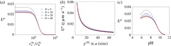
Written in dimensional form (see figure 6),
 $$\begin{eqnarray}\bar{\boldsymbol{U}}^{e}=-\frac{1}{3}\left(\frac{k_{B}T}{e}\right)^{2}\frac{\unicode[STIX]{x1D716}}{\unicode[STIX]{x1D702}}\frac{A_{1}\unicode[STIX]{x0394}k_{eff}^{(h)}c_{hp}^{\infty }}{D_{h}\left(c_{h}^{\infty }+c_{s}^{\infty }\right)}\left[\frac{e\bar{\unicode[STIX]{x1D701}}_{0}}{k_{B}T}+4\ln \cosh \left(\frac{e\bar{\unicode[STIX]{x1D701}}_{0}}{4k_{B}T}\right)\right]\hat{\boldsymbol{e}}_{z},\end{eqnarray}$$
where
 $\bar{\unicode[STIX]{x1D701}}_{0}=(k_{B}T/e)\unicode[STIX]{x1D701}_{0}$
is the average swimmer
 $\unicode[STIX]{x1D701}$
potential. A plot of this electrophoretic contribution against the solution salt concentration (ionic strength) is shown in figure 6(a). As expected, this contribution is strongly sensitive to salt concentration. Interestingly, the swimmer speed is only weakly dependent on pH (see figure 6
c) under weakly acidic conditions (high
 $c_{h}^{\infty }$
). This is due to the competition between the dependence on
 $c_{h}^{\infty }$
of
 $A_{1}$
(decreases with
 $c_{h}$
),
 $\unicode[STIX]{x1D707}_{e}$
(increases with
 $c_{h}$
) and the denominator of the expression for
 $\boldsymbol{U}^{e}$
(increases with
 $c_{h}$
). This is consistent with recent experiments (Brown & Poon Reference Brown and Poon2014) which showed a minor reduction of swimming speed on addition of sodium hydroxide (NaOH). Furthermore, the propulsion speed is inversely dependent on swimmer size,
 $a$
for large swimmer sizes as shown in figure 6(b). This is consistent with the experimental observation of
 ${\sim}1/a$
propulsion velocity decay for large swimmer sizes (Howse et al.
Reference Howse, Jones, Ryan, Gough, Vafabakhsh and Golestanian2007).
(Electrophoretic and ionic-diffusiophoretic contributions) (a) the propulsion speed
 $U^{e}$
as a function of the salt concentration
 $C_{s}^{\infty }$
. (b) The propulsion speed
 $U^{e}$
decays with increasing size
 $a$
. (c) The speed
 $U^{e}$
against the solution pH (we expect that the charge balance may be more complicated and the reaction kinetics are known to change with the solution pH (McKee Reference McKee1969; Liu et al.
Reference Liu, Wu, Li, Yin and Nie2014)).

3.2 Self-diffusiophoresis
In this section, we outline a solution of the equations of motion for the neutral solutes in the outer region
 $(\unicode[STIX]{x1D712}=L_{eff}/a\rightarrow 0)$
to calculate the neutral-diffusiophoretic contribution to the propulsion velocity,
 $\boldsymbol{U}^{d}$
. Detailed calculations for the inner interaction layer where the fields vary on the length scale
 $L_{eff}$
can be found in the literature (Anderson et al.
Reference Anderson, Lowell and Prieve1982; Golestanian et al.
Reference Golestanian, Liverpool and Ajdari2005, Reference Golestanian, Liverpool and Ajdari2007; Howse et al.
Reference Howse, Jones, Ryan, Gough, Vafabakhsh and Golestanian2007; Michelin & Lauga Reference Michelin and Lauga2014).
Here since there is a finite propulsion velocity,
 $\bar{\boldsymbol{U}}^{d}\neq 0$
, for the uniformly coated system,
 $k_{i}^{(0)}\neq 0,k_{i}^{(1)}=0$
, then a weak variation of rates due to a varying thickness
 $k_{i}^{(0)}\gg k_{i}^{(1)}$
leads to a small correction which we can ignore. Hence we set
 $k_{i}^{(1)}=0$
for the rest of this section.
3.2.1 Dimensionless equations
The position vector
 $\bar{\boldsymbol{r}}$
is measured in units of the swimmer size ‘
 $a$
’, concentrations
 $\bar{c}_{i}$
in units of the steady-state background values
 $c_{i}^{\infty }$
(note that
 $\bar{c}_{o}$
is measured in units of
 $c_{hp}^{\infty }$
), the short-ranged interaction potential of solutes with the Janus sphere,
 $\bar{\unicode[STIX]{x1D6F9}}$
in terms of the thermal energy scale
 $\unicode[STIX]{x1D6FD}^{-1}=k_{B}T$
, neutral solute fluxes,
 $\bar{\boldsymbol{J}}_{n}$
in units of
 $D_{n}c_{hp}^{\infty }/a$
, with
 $D_{i}$
the diffusion coefficient of the
 $i$
th solute. The fluid flow velocity
 $\bar{\boldsymbol{v}}$
is rescaled by
 $\bar{\unicode[STIX]{x1D707}}_{d}^{\ddagger }c_{hp}^{\infty }/a$
, where
 $\bar{\unicode[STIX]{x1D707}}_{d}^{\ddagger }$
is the characteristic diffusiophoretic mobility, the pressure
 $\bar{p}$
is rescaled by
 $\bar{\unicode[STIX]{x1D707}}_{d}^{\ddagger }\unicode[STIX]{x1D702}c_{hp}^{\infty }/a^{2}$
. Hence, the dimensionless quantities (no overbar) are expressed in terms of dimensional ones (with overbar) as follows
 $\boldsymbol{r}=(x,y,z)=\bar{\boldsymbol{r}}/a,c_{i}=\bar{c}_{i}/c_{i}^{\infty },\unicode[STIX]{x1D6F9}=\unicode[STIX]{x1D6FD}\bar{\unicode[STIX]{x1D6F9}},\boldsymbol{v}=\bar{\boldsymbol{v}}a/c_{hp}^{\infty }\bar{\unicode[STIX]{x1D707}}_{d}^{\ddagger },p=\bar{p}a^{2}/c_{hp}^{\infty }\bar{\unicode[STIX]{x1D707}}_{d}^{\ddagger }\unicode[STIX]{x1D702}$
. As before we define the dimensionless difference of the concentrations from their bulk values as
 $C_{i}(\boldsymbol{r})\equiv c_{i}(\boldsymbol{r})-1=(\bar{c}_{i}/c_{i}^{\infty })-1$
.
The dimensionless equations for
 $r>1$
in the outer region are thus Laplace equations for the concentration deviations
 $$\begin{eqnarray}\displaystyle & \displaystyle \unicode[STIX]{x1D6FB}^{2}C_{o}=0, & \displaystyle\end{eqnarray}$$
 $$\begin{eqnarray}\displaystyle & \displaystyle \unicode[STIX]{x1D6FB}^{2}C_{hp}=0, & \displaystyle\end{eqnarray}$$
and the Stokes equations for the fluid velocity,
 $\boldsymbol{v}(\boldsymbol{r})$
 $$\begin{eqnarray}\displaystyle \mathbf{0}=\unicode[STIX]{x1D735}\boldsymbol{\cdot }\unicode[STIX]{x1D72B}=\unicode[STIX]{x1D6FB}^{2}\boldsymbol{v}-\unicode[STIX]{x1D735}p;\quad 0=\unicode[STIX]{x1D735}\boldsymbol{\cdot }\boldsymbol{v}, & & \displaystyle\end{eqnarray}$$
where
 $p(\boldsymbol{r})$
is the hydrostatic pressure at
 $\boldsymbol{r}$
(Anderson Reference Anderson1989; Golestanian et al.
Reference Golestanian, Liverpool and Ajdari2005, Reference Golestanian, Liverpool and Ajdari2007; Howse et al.
Reference Howse, Jones, Ryan, Gough, Vafabakhsh and Golestanian2007; Michelin & Lauga Reference Michelin and Lauga2014).
3.2.2 Dimensionless boundary conditions
Matching with the inner layer (Anderson Reference Anderson1989; Golestanian et al. Reference Golestanian, Liverpool and Ajdari2005, Reference Golestanian, Liverpool and Ajdari2007; Howse et al. Reference Howse, Jones, Ryan, Gough, Vafabakhsh and Golestanian2007; Michelin & Lauga Reference Michelin and Lauga2014), gives rise to non-zero flux boundary conditions for hydrogen peroxide and oxygen
 $$\begin{eqnarray}\displaystyle & \displaystyle \left.-\unicode[STIX]{x2202}_{r}C_{o}\right|_{r=1}={\mathcal{J}}_{o}(\unicode[STIX]{x1D703})K(\cos \unicode[STIX]{x1D703})=\frac{D_{hp}}{2D_{o}}{\mathcal{K}}_{eff}^{(hp)}(1+C_{hp})K(\cos \unicode[STIX]{x1D703}), & \displaystyle\end{eqnarray}$$
 $$\begin{eqnarray}\displaystyle & \displaystyle \left.-\unicode[STIX]{x2202}_{r}C_{hp}\right|_{r=1}={\mathcal{J}}_{hp}(\unicode[STIX]{x1D703})K(\cos \unicode[STIX]{x1D703})=-{\mathcal{K}}_{eff}^{(hp)}(1+C_{hp})K(\cos \unicode[STIX]{x1D703}), & \displaystyle\end{eqnarray}$$
and vanishing concentration deviations far from the swimmer
 $C_{o},C_{hp}\rightarrow 0$
as
 $r\rightarrow \infty$
.
 $K(\cos \unicode[STIX]{x1D703})$
, the catalyst coverage function, is
 $1$
on the platinum hemisphere and zero on the polystyrene hemisphere. From the reaction kinetics in appendix A, we obtain non-zero fluxes for hydrogen peroxide and oxygen
 $$\begin{eqnarray}\displaystyle & \displaystyle {\mathcal{J}}_{o}(\unicode[STIX]{x1D703})=\frac{1}{2}\left(\frac{k_{eff}^{(hp)}\bar{c}_{hp}a}{D_{o}c_{hp}^{\infty }}\right)K(\cos \unicode[STIX]{x1D703})=\frac{D_{hp}}{2D_{o}}{\mathcal{K}}_{eff}^{(hp)}(1+C_{hp}(1,\unicode[STIX]{x1D703}))K(\cos \unicode[STIX]{x1D703}), & \displaystyle\end{eqnarray}$$
 $$\begin{eqnarray}\displaystyle & \displaystyle {\mathcal{J}}_{hp}(\unicode[STIX]{x1D703})=-\left(\frac{k_{eff}^{(hp)}\bar{c}_{hp}a}{D_{hp}c_{hp}^{\infty }}\right)K(\cos \unicode[STIX]{x1D703})=-{\mathcal{K}}_{eff}^{(hp)}(1+C_{hp}(1,\unicode[STIX]{x1D703}))K(\cos \unicode[STIX]{x1D703}). & \displaystyle\end{eqnarray}$$
We have defined dimensionless
 ${\mathcal{K}}_{eff}^{(hp)}=k_{eff}^{(hp)}a/D_{hp}$
, where
 $k_{eff}^{(hp)}\bar{c}_{hp}>0$
is the effective rate of consumption of the hydrogen peroxide (see appendix A for details of the derivation).
The boundary conditions for the fluid velocity are
 $$\begin{eqnarray}\boldsymbol{v}|_{r=1}=\boldsymbol{U}^{d}+\boldsymbol{v}_{slip}^{d};\quad \boldsymbol{v}(r\rightarrow \infty )=\mathbf{0},\end{eqnarray}$$
where
 $\boldsymbol{U}^{d}$
is the neutral self-diffusiophoretic contribution to the propulsion velocity.
 is the self-diffusiophoretic slip velocity obtained by matching with the inner solution (Anderson et al.
Reference Anderson, Lowell and Prieve1982; Anderson Reference Anderson1989) and
 is a unit matrix. The dimensionless self-diffusiophoretic mobility is given by
 $\unicode[STIX]{x1D707}_{d}^{(i)}=\lim _{\unicode[STIX]{x1D70C}^{\prime }\rightarrow \infty }\int _{0}^{\unicode[STIX]{x1D70C}^{\prime }}\unicode[STIX]{x1D70C}[1-e^{-\unicode[STIX]{x1D6F9}_{i}(\unicode[STIX]{x1D70C})}]\,\text{d}\unicode[STIX]{x1D70C}$
(Anderson Reference Anderson1989).
Finally, the zero total force condition on the swimmer
 $$\begin{eqnarray}\boldsymbol{F}=\oint _{r=1}\unicode[STIX]{x1D72B}\boldsymbol{\cdot }\hat{\boldsymbol{n}}\sin \unicode[STIX]{x1D703}\,\text{d}\unicode[STIX]{x1D703}=\mathbf{0},\end{eqnarray}$$
determines the diffusiophoretic propulsion velocity
 $\boldsymbol{U}^{d}$
.
3.2.3 Outer concentration fields
The general solution of the Laplace equations (3.52), (3.53) for the neutral solutes is of the form
 $$\begin{eqnarray}\displaystyle & \displaystyle C_{o}(r,\unicode[STIX]{x1D703})=\mathop{\sum }_{l=0}^{\infty }\left(\frac{D_{hp}}{2D_{o}}\right)W_{l}\frac{P_{l}(\cos \unicode[STIX]{x1D703})}{r^{l+1}}, & \displaystyle\end{eqnarray}$$
 $$\begin{eqnarray}\displaystyle & \displaystyle C_{hp}(r,\unicode[STIX]{x1D703})=-\mathop{\sum }_{l=0}^{\infty }W_{l}\frac{P_{l}(\cos \unicode[STIX]{x1D703})}{r^{l+1}}, & \displaystyle\end{eqnarray}$$
where
 $P_{l}(\cos \unicode[STIX]{x1D703})$
are the Legendre polynomials and note that we have used the fact that
 $D_{hp}{\mathcal{J}}_{hp}+2D_{o}{\mathcal{J}}_{o}=0$
. The amplitudes,
 $W_{l}$
, are determined from either of the boundary conditions;
 $$\begin{eqnarray}\displaystyle & \displaystyle \left.-\unicode[STIX]{x2202}_{r}C_{o}\right|_{r=1}=\frac{D_{hp}}{2D_{o}}{\mathcal{K}}_{eff}^{(hp)}(1+C_{hp})K(\cos \unicode[STIX]{x1D703}), & \displaystyle\end{eqnarray}$$
 $$\begin{eqnarray}\displaystyle & \displaystyle \left.-\unicode[STIX]{x2202}_{r}C_{hp}\right|_{r=1}=-{\mathcal{K}}_{eff}^{(hp)}(1+C_{hp})K(\cos \unicode[STIX]{x1D703}). & \displaystyle\end{eqnarray}$$
This gives rise to a system of equations:
 $$\begin{eqnarray}\mathop{\sum }_{l=0}^{\infty }W_{l}(l+1)P_{l}(\cos \unicode[STIX]{x1D703})={\mathcal{K}}_{eff}^{(hp)}\left(1-\mathop{\sum }_{l=0}^{\infty }W_{l}P_{l}(\cos \unicode[STIX]{x1D703})\right)K(\cos \unicode[STIX]{x1D703}).\end{eqnarray}$$
From this, using the orthogonality condition of the Legendre polynomials, we obtain the linear system of equations for the amplitudes,
 $W_{l}$
:
 $$\begin{eqnarray}\displaystyle \unicode[STIX]{x1D648}^{(d)}\boldsymbol{\cdot }\boldsymbol{W}=\unicode[STIX]{x1D726}^{(d)}, & & \displaystyle\end{eqnarray}$$
where
 $\boldsymbol{W}=(W_{0},\ldots ,W_{l},\ldots )$
, and more explicitly
 $$\begin{eqnarray}\left(\begin{array}{@{}cccccc@{}}1 & 0 & 0 & \cdots \, & 0 & \cdots \\ 0 & M_{11}^{(d)} & M_{12}^{(d)} & \cdots \, & M_{1l}^{(d)} & \cdots \\ 0 & M_{21}^{(d)} & M_{22}^{(d)} & \cdots \, & M_{2l}^{(d)} & \cdots \\ \vdots & \vdots & \vdots & \ddots & \vdots & \ldots \\ 0 & M_{n1}^{(d)} & M_{n2}^{(d)} & \ldots & M_{nl}^{(d)} & \ldots \\ \vdots & \vdots & \vdots & \vdots & \vdots & \ddots \end{array}\right)\left(\begin{array}{@{}c@{}}W_{0}\\ W_{1}\\ W_{2}\\ \vdots \\ W_{l}\\ \vdots \end{array}\right)=\left(\begin{array}{@{}c@{}}0\\ \unicode[STIX]{x1D6EC}_{1}^{(d)}\\ \unicode[STIX]{x1D6EC}_{2}^{(d)}\\ \vdots \\ \unicode[STIX]{x1D6EC}_{n}^{(d)}\\ \vdots \end{array}\right),\end{eqnarray}$$
where the matrix
 $\unicode[STIX]{x1D648}^{(d)}$
and vector
 $\unicode[STIX]{x1D726}^{(d)}$
entries are given by
 $$\begin{eqnarray}\displaystyle & \displaystyle M_{nl}^{(d)}=\unicode[STIX]{x1D6FF}_{nl}+{\mathcal{K}}_{eff}^{(hp)}\left(\frac{n+\frac{1}{2}}{n+1}\right)\int _{0}^{1}P_{n}(x)P_{l}(x)\,\text{d}x, & \displaystyle\end{eqnarray}$$
 $$\begin{eqnarray}\displaystyle & \displaystyle \unicode[STIX]{x1D6EC}_{n}^{(d)}={\mathcal{K}}_{eff}^{(hp)}\left(\frac{n+\frac{1}{2}}{n+1}\right)\int _{0}^{1}P_{n}(x)\,\text{d}x. & \displaystyle\end{eqnarray}$$
Here as in the ionic section, we solve a truncated approximation of the linear equations above, including all modes up to the
 $N$
th Legendre mode
 $\{W_{0},W_{1},\ldots ,W_{N}\}$
. As above, we can obtain analytic asymptotic solutions for
 ${\mathcal{K}}_{eff}^{(hp)}\ll 1$
and
 ${\mathcal{K}}_{eff}^{(hp)}\gg 1$
:
 ${\mathcal{K}}_{eff}^{(hp)}\ll 1$
: In this regime,
 $W_{l}\sim \unicode[STIX]{x1D6EC}_{l}^{(d)}$
and
 $$\begin{eqnarray}W_{1}\sim {\textstyle \frac{3}{8}}{\mathcal{K}}_{eff}^{(hp)}\end{eqnarray}$$
 ${\mathcal{K}}_{eff}^{(hp)}\gg 1$
: In this regime,
 $$\begin{eqnarray}W_{1}\sim \unicode[STIX]{x1D6EF},\end{eqnarray}$$
where
 $\unicode[STIX]{x1D6EF}>0$
is some constant to be determined numerically. Since
 ${\mathcal{K}}_{eff}^{(hp)}\propto a$
(swimmer size), this implies the limit
 ${\mathcal{K}}_{eff}^{(hp)}\gg 1$
corresponds to large swimmer size. For
 $a=1.00~\unicode[STIX]{x03BC}\text{m}$
sized swimmer in 10 % w/v
 $\text{H}_{2}\text{O}_{2}$
solution, and the measured reaction rates in table 1, the estimate of the dimensionless reaction rate coefficient is
 ${\mathcal{K}}_{eff}^{(hp)}\approx 0.026$
. Hence, this puts the current experimental measurements (Brown & Poon Reference Brown and Poon2014; Ebbens et al.
Reference Ebbens, Gregory, Dunderdale, Howse, Ibrahim, Liverpool and Golestanian2014) in the first regime
 $(W_{l}\sim \unicode[STIX]{x1D6EC}_{l}^{(d)})$
. We note that in this regime
 $C_{hp}\sim W_{l}\sim {\mathcal{K}}_{eff}^{(hp)}\ll 1$
.
The coefficients
 $W_{l}$
determine the solute concentration, and hence the slip velocity which act as boundary conditions for the Stokes flow problem. Hence the velocity fields generated, expressed in terms of the fundamental singularities (see (3.48)) of the Stokes flow are
 $$\begin{eqnarray}\displaystyle \boldsymbol{v}(\boldsymbol{r})=B_{1}^{(d)}\boldsymbol{D}(\boldsymbol{r})+B_{3}^{(d)}[\unicode[STIX]{x2202}_{z}^{2}\boldsymbol{G}(\boldsymbol{r})]+O(r^{-4}), & & \displaystyle\end{eqnarray}$$
where the coefficients (
 $B_{1}^{(d)},B_{3}^{(d)}$
) are
 $$\begin{eqnarray}B_{1}^{(d)}=-\frac{1}{3}\unicode[STIX]{x1D707}_{d}W_{1}\left(1-\frac{3}{2}\frac{W_{3}}{W_{1}}\right);\quad B_{3}^{(d)}=\frac{5}{4}\unicode[STIX]{x1D707}_{d}W_{3}.\end{eqnarray}$$
Imposing the condition of net zero total force, we obtain the neutral-diffusiophoretic contribution to the propulsion velocity as

where since we have taken the interaction potential,
 $\unicode[STIX]{x1D6F9}$
identical for all species, we have identical neutral-diffusiophoretic mobilities for all the neutral solute species,
 $\unicode[STIX]{x1D707}_{d}^{(i)}=1,i\in \{o,hp\}$
. From the modes calculated above, we thus obtain
 $$\begin{eqnarray}\boldsymbol{U}^{d}=-{\textstyle \frac{2}{3}}\unicode[STIX]{x1D707}_{d}W_{1}\hat{\boldsymbol{e}}_{z},\end{eqnarray}$$
where
 $\unicode[STIX]{x1D707}_{d}=\unicode[STIX]{x1D707}_{d}^{(hp)}-(D_{hp}/2D_{o})\unicode[STIX]{x1D707}_{d}^{(o)}=1-(D_{hp}/2D_{o})$
is the combined effective diffusiophoretic mobility.
3.3 Comparison of ionic and neutral velocities
Finally, we can now compare the two contributions to the swimmer propulsion from ionic and neutral solutes using dimensional quantities. From (3.50) and (3.75), the relative speed
 $$\begin{eqnarray}\frac{\bar{U}^{e}}{\bar{U}^{d}}=\frac{\left(\unicode[STIX]{x1D716}k_{B}^{2}T^{2}/a\unicode[STIX]{x1D702}e^{2}\right)U^{e}}{\left(\bar{\unicode[STIX]{x1D707}}_{d}^{\ddagger }c_{hp}^{\infty }/a\right)U^{d}}=\frac{\bar{\unicode[STIX]{x1D707}}_{e}}{\bar{\unicode[STIX]{x1D707}}_{d}}\frac{(k_{B}T/e)\unicode[STIX]{x1D6FE}^{(1)}A_{1}}{c_{hp}^{\infty }W_{1}},\end{eqnarray}$$
where
 $\bar{\unicode[STIX]{x1D707}}_{e}=(\unicode[STIX]{x1D716}k_{B}T/e\unicode[STIX]{x1D702})\,\unicode[STIX]{x1D707}_{e}$
is the electrophoretic mobility and
 $\bar{\unicode[STIX]{x1D707}}_{d}=\unicode[STIX]{x1D707}_{d}\bar{\unicode[STIX]{x1D707}}_{d}^{\ddagger }$
is the diffusiophoretic mobility, both in dimensional form. For a fixed swimmer size, and in the limit
 $\unicode[STIX]{x1D6FE}^{(0)}\ll 1,{\mathcal{K}}_{eff}^{(hp)}\ll 1$
, the above ratio takes the simple analytic expression
 $$\begin{eqnarray}\frac{\bar{U}^{e}}{\bar{U}^{d}}=\frac{1}{6}\frac{\bar{\unicode[STIX]{x1D707}}_{e}}{\bar{\unicode[STIX]{x1D707}}_{d}}\frac{D_{hp}}{D_{h}}\frac{\unicode[STIX]{x0394}k_{eff}^{(h)}}{k_{eff}^{(hp)}}\frac{\left(k_{B}T/e\right)}{(c_{s}^{\infty }+c_{h}^{\infty })},\end{eqnarray}$$
where
 $k_{eff}^{(hp)}c_{hp}^{\infty }>0$
is the effective rate of the hydrogen peroxide consumption and
 $\unicode[STIX]{x0394}k_{eff}^{(h)}>0$
is the scale of the difference between the rates at the pole and equator due to the Pt thickness variation (defined in appendix A for a particular example of reaction model). These rates are linear functions of the
 $c_{hp}^{\infty }$
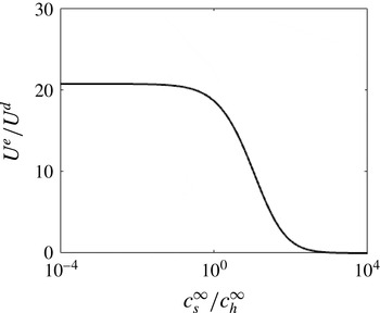
concentration for low fuel concentration. In figure 7, it can be seen that the electrophoretic contribution vanishes at large ionic strengths and the swimmer speed asymptotically approaches the diffusiophoretic contribution value
 $\bar{U}^{d}$
. The self-diffusiophoretic speed
 $\bar{U}^{d}=\bar{\unicode[STIX]{x1D707}}_{d}k_{eff}^{(hp)}c_{hp}^{\infty }/4D_{hp}\sim 0.52~\unicode[STIX]{x03BC}\text{ms}^{-1}$
(see table 1) for the chosen system parameter values in the plot (figure 7).


Asymptotic regimes of the swimmer propulsion speed
 $\bar{U}$
. The dimensionless parameters on the horizontal axes are
 $\unicode[STIX]{x1D6FE}^{(0)}=k_{eff}^{(h)}c_{hp}^{\infty }a/D_{h}\sum _{i\in \,ions}c_{i}^{\infty }$
and
 ${\mathcal{K}}_{eff}^{(hp)}=k_{eff}^{(hp)}a/D_{hp}$
where
 $D_{i}$
and
 $c_{i}^{\infty }$
are respectively the diffusion coefficient and bulk concentration of chemical species
 $i$
.
 $k_{eff}^{(i)}$
is the average rate of production/consumption of species
 $i$
on the catalytic coated hemisphere.
 $\unicode[STIX]{x0394}k_{eff}^{(i)}$
is the difference in the reaction rate between the equator where the coating is thinnest and the pole where the coating is thickest.
 $\bar{\unicode[STIX]{x1D707}}_{e}$
and
 $\bar{\unicode[STIX]{x1D707}}_{d}$
are electrophoretic and diffusiophoretic mobilities respectively.

4 Summary and discussion
The total propulsion velocity of the metallic-insulator sphere from both electrophoresis and diffusiophoresis, from (3.50) and (3.75), in dimensional form is
 $$\begin{eqnarray}\bar{\boldsymbol{U}}=-\left[\frac{1}{3}\bar{\unicode[STIX]{x1D707}}_{e}\frac{\unicode[STIX]{x0394}k_{eff}^{(h)}c_{hp}^{\infty }}{D_{h}\left(c_{s}^{\infty }+c_{h}^{\infty }\right)}\left(\frac{k_{B}T}{e}\right)A_{1}+\frac{2}{3}\bar{\unicode[STIX]{x1D707}}_{d}\frac{c_{hp}^{\infty }}{a}W_{1}\right]\hat{\boldsymbol{e}}_{z},\end{eqnarray}$$
where
 $\bar{\unicode[STIX]{x1D707}}_{e}$
and
 $\bar{\unicode[STIX]{x1D707}}_{d}$
are the electrophoretic and diffusiophoretic mobilities. The scale of the difference between the rates at the poles and equator due to the Pt thickness variation
 $\unicode[STIX]{x0394}k_{eff}^{(h)}>0$
is defined in appendix A for a particular reaction kinetic model. We point out that these results are qualitatively independent of the details of the reaction kinetics, provided the reaction involves both charged and neutral pathways for the reduction of the hydrogen peroxide and the reaction rate varies along the catalytic cap.
The ionic contribution to the expression above has a number of important simple features that are in agreement with recent experimental results on this system (Howse et al.
Reference Howse, Jones, Ryan, Gough, Vafabakhsh and Golestanian2007; Ebbens et al.
Reference Ebbens, Tu, Howse and Golestanian2012; Brown & Poon Reference Brown and Poon2014; Ebbens et al.
Reference Ebbens, Gregory, Dunderdale, Howse, Ibrahim, Liverpool and Golestanian2014; Das et al.
Reference Das, Garg, Campbell, Howse, Sen, Velegol, Golestanian and Ebbens2015): (i) it depends linearly on the fuel,
 $c_{hp}^{\infty }$
, at low concentrations and the dependence weakens at high concentrations, (ii) it is independent of
 $a$
at small
 $a$
and behaves as
 $1/a$
for large
 $a$
due to fuel depletion as shown in Ebbens et al. (Reference Ebbens, Tu, Howse and Golestanian2012) and (iii) it is a monotonically decreasing function of salt concentration,
 $c_{s}^{\infty }$
starting from a finite value when
 $c_{s}^{\infty }=0$
and tending to zero as
 $c_{s}^{\infty }$
becomes large. Hence at high salt concentration the swimming speed saturates to the neutral-diffusiophoretic value (see figure 7). The electrophoretic contribution, which can be much larger than the diffusiophoretic part, vanishes if there is no variation in the rates
 $k_{i}$
on the surface.
Adding salt to the solution containing the swimmer would influence the propulsion in three possible ways (i) pH neutral salts that do not specifically adsorb to the surface would enhance the solution conductivity thereby reducing the effective screening length (ii) while alkali or acidic salts would in general alter the total surface charge in addition to the increased solution conductivity, (iii) Pt catalytic decomposition of
 $\text{H}_{2}\text{O}_{2}$
is known to strongly depend on the solution pH (McKee Reference McKee1969; Liu et al.
Reference Liu, Wu, Li, Yin and Nie2014). Hence, non-pH neutral salts would also affect the Pt catalytic activity.
We note also that due to the existence of the two separate reaction loops, the overall catalytic reaction rate (measured from the current
 $J_{o}$
above) can be significantly reduced with only small reductions to the swimming speed; say by a significant decrease in
 $k_{1}$
. This type of behaviour would be expected from any reaction scheme which has this topological structure.
In conclusion, we have shown that in a system with catalytic reaction with charged intermediates, the existence of thickness dependence in the reaction rates up to a certain limit (a few nanometres), allows us to create – by tapering the catalyst layer – spatially separated non-equilibrium cycles that could lead to large-scale (many microns) ionic currents in the form of closed loops in the bulk. This remarkable effect, combining long-range electrostatic interactions with non-equilibrium chemical reactions to substantially enhance surface generated flows has potential for application in many different areas of nanoscience.
Acknowledgements
This work was supported by EPSRC grant EP/G026440/1 (T.B.L., Y.I.), and HFSP grant RGP0061/2013 (R.G.). Y.I. acknowledges the support of University of Bristol. T.B.L. acknowledges support of BrisSynBio, a BBSRC/EPSRC Advanced Synthetic Biology Research Centre (grant no. BB/L01386X/1).
Appendix A. Reaction kinetics
In this section, our goal is to obtain the fluxes on the surface of the swimmer,
 $\bar{{\mathcal{J}}}_{i}$
of all the chemical species involved in the
 $\text{H}_{2}\text{O}_{2}$
decomposition
 $$\begin{eqnarray}\text{Pt}+2\text{H}_{2}\text{O}_{2}\rightarrow \displaystyle \text{Intermediate complexes}\rightarrow \text{Pt}+2\text{H}_{2}\text{O}+\text{O}_{2}.\end{eqnarray}$$
Though a complete picture of the intermediate complexes in reaction (A 1) remains elusive, it is known that there are neutral pathways as well as ionic electrochemical pathways (Hall, Khudaish & Hart Reference Hall, Khudaish and Hart2000; Katsounaros et al. Reference Katsounaros, Schneider, Meier, Benedikt, Biedermann, Auer and Mayrhofer2012). However, we find that our results are qualitatively independent of many details of the reaction scheme considered as long as they involve both neutral and charged pathways. So our lack of knowledge of the microscopic chemical kinetics is not such a hindrance. To illustrate this, we consider two different reaction schemes involving a neutral as well as a charged pathway. We emphasize that both schemes are provided simply as examples as the precise details of the chemical kinetics are not known.
A.1 Reaction scheme 1
First, we consider a reaction scheme for the reaction (A 1) made up of two pathways, one neutral
 $$\begin{eqnarray}\text{Pt}+2\text{H}_{2}\text{O}_{2}\overset{k_{0}}{\longrightarrow }\text{Pt}\left(\text{H}_{2}\text{O}_{2}\right)+\text{H}_{2}\text{O}_{2}\overset{k_{1}}{\rightarrow }\text{Pt}\left(\text{H}_{2}\text{O}_{2}\right)_{2}\overset{k_{2}}{\rightarrow }\text{Pt}+2\text{H}_{2}\text{O}+\text{O}_{2},\end{eqnarray}$$
and the other ionic involving charged intermediates,
 $$\begin{eqnarray}\displaystyle \text{Pt}+2\text{H}_{2}\text{O}\underset{k_{-3}}{\overset{k_{3}}{\rightleftharpoons }}\text{Pt}\left(\text{H}_{2}\text{O}_{2}\right)+2e^{-}+2\text{H}^{+}. & & \displaystyle\end{eqnarray}$$
(Reaction scheme 1): schematic complexation kinetics of the platinum catalyst with free (
 $0$
th state) Pt occupied with probability density
 $p_{0}$
; first complex state
 $\text{Pt}(\text{H}_{2}\text{O}_{2})$
occupied with probability density
 $p_{1}$
and the second complex state
 $\text{Pt}(\text{H}_{2}\text{O}_{2})_{2}$
occupied with probability density
 $p_{2}$
.

The reaction scheme above and the intermediate states denoted by
 $(0,1,2)$
are enumerated in figure 9. The kinetics of the Pt catalyst complexation in stationary state reads
 $$\begin{eqnarray}\displaystyle & \displaystyle 0=\unicode[STIX]{x2202}_{t}p_{0}=-k_{0}\bar{c}_{hp}p_{0}-k_{3}p_{0}+k_{2}p_{2}+k_{-3}\bar{c}_{h}^{2}p_{1}, & \displaystyle\end{eqnarray}$$
 $$\begin{eqnarray}\displaystyle & \displaystyle 0=\unicode[STIX]{x2202}_{t}p_{1}=k_{0}\bar{c}_{hp}p_{0}+k_{3}p_{0}-k_{1}\bar{c}_{hp}p_{1}-k_{-3}\bar{c}_{h}^{2}p_{1}, & \displaystyle\end{eqnarray}$$
 $$\begin{eqnarray}\displaystyle & \displaystyle 0=\unicode[STIX]{x2202}_{t}p_{2}=k_{1}\bar{c}_{hp}p_{1}-k_{2}p_{2}, & \displaystyle\end{eqnarray}$$
where
 $p_{i}$
are the complexation probabilities. Solving for these probabilities
 $p_{i}$
, we obtain
 $$\begin{eqnarray}\displaystyle & \displaystyle p_{0}={\mathcal{M}}^{-1}k_{2}\left(k_{1}\bar{c}_{hp}+k_{-3}\bar{c}_{h}^{2}\right), & \displaystyle\end{eqnarray}$$
 $$\begin{eqnarray}\displaystyle & \displaystyle p_{1}={\mathcal{M}}^{-1}k_{2}\left(k_{0}\bar{c}_{hp}+k_{3}\right), & \displaystyle\end{eqnarray}$$
 $$\begin{eqnarray}\displaystyle & \displaystyle p_{2}={\mathcal{M}}^{-1}k_{1}\bar{c}_{hp}\left(k_{0}\bar{c}_{hp}+k_{3}\right), & \displaystyle\end{eqnarray}$$
where the normalization condition
 $p_{0}+p_{1}+p_{2}=1$
was used and we have defined
 $$\begin{eqnarray}{\mathcal{M}}:=k_{2}k_{3}+k_{2}k_{-3}\bar{c}_{h}^{2}+\left(k_{0}k_{2}+k_{1}k_{3}+k_{1}k_{2}\right)\bar{c}_{hp}+k_{0}k_{1}\bar{c}_{hp}^{2}.\end{eqnarray}$$
This leads to expressions for the fluxes
 $\bar{{\mathcal{J}}}_{i}$
of
 $i\in \{o,hp,h\}$
 $$\begin{eqnarray}\displaystyle \bar{{\mathcal{J}}}_{o}(\unicode[STIX]{x1D703}) & = & \displaystyle k_{2}p_{2}K(\cos \unicode[STIX]{x1D703}),\nonumber\\ \displaystyle & = & \displaystyle {\mathcal{M}}^{-1}k_{1}k_{2}\bar{c}_{hp}(k_{0}\bar{c}_{hp}+k_{3})K(\cos \unicode[STIX]{x1D703}),\end{eqnarray}$$
 $$\begin{eqnarray}\displaystyle \bar{{\mathcal{J}}}_{hp}(\unicode[STIX]{x1D703}) & = & \displaystyle -\!\left(k_{0}p_{0}+k_{1}p_{1}\right)\bar{c}_{hp}K(\cos \unicode[STIX]{x1D703}),\nonumber\\ \displaystyle & = & \displaystyle -{\mathcal{M}}^{-1}k_{2}\bar{c}_{hp}(k_{1}k_{3}+k_{0}k_{-3}\bar{c}_{h}^{2}+2k_{0}k_{1}\bar{c}_{hp})K(\cos \unicode[STIX]{x1D703}),\end{eqnarray}$$
 $$\begin{eqnarray}\displaystyle \bar{{\mathcal{J}}}_{h}(\unicode[STIX]{x1D703}) & = & \displaystyle 2\left(k_{3}p_{0}-k_{-3}\bar{c}_{h}^{2}p_{1}\right)K(\cos \unicode[STIX]{x1D703}),\nonumber\\ \displaystyle & = & \displaystyle 4{\mathcal{M}}^{-1}k_{2}\bar{c}_{hp}(k_{1}k_{3}-k_{0}k_{-3}\bar{c}_{h}^{2})K(\cos \unicode[STIX]{x1D703}),\end{eqnarray}$$
and for the fluxes of hydroxide and the salt,
 $\bar{{\mathcal{J}}}_{oh}=0,\bar{{\mathcal{J}}}_{s,\pm }=0$
. Measurements of the reaction rates (Ebbens et al.
Reference Ebbens, Gregory, Dunderdale, Howse, Ibrahim, Liverpool and Golestanian2014) imply that
 $\bar{{\mathcal{J}}}_{hp}$
and
 $\bar{{\mathcal{J}}}_{o}$
vary with the Pt coating thickness (of
 ${\sim}$
nm scale). Hence we may assume that the rate ‘constants’
 $k_{i}$
vary in a similar manner.
Since the thickness of the coating varies across the Pt cap, the reaction rates
 $k_{i}(\unicode[STIX]{x1D703})$
vary over the coated hemisphere, and can be expanded in Legendre polynomials. We consider a simple linear approximation
 $$\begin{eqnarray}k_{i}(\unicode[STIX]{x1D703})\cong k_{i}^{(0)}+k_{i}^{(1)}\cos \unicode[STIX]{x1D703},\end{eqnarray}$$
in
 $\cos \unicode[STIX]{x1D703}$
and we assume a weak variation
 $k_{i}^{(1)}/k_{i}^{(0)}\ll 1$
of the rates.
The solute fluxes
 $\bar{{\mathcal{J}}}_{i}$
above in (A 11)–(A 13) require the inner (Debye-layer) proton concentration profile
 $$\begin{eqnarray}\bar{c}_{h}(1,\unicode[STIX]{x1D703})/c_{h}^{\infty }=\left(1+C_{h}(1,\unicode[STIX]{x1D703})\right)e^{-\unicode[STIX]{x1D701}(\unicode[STIX]{x1D703})};\quad \unicode[STIX]{x1D701}(\unicode[STIX]{x1D703})=\unicode[STIX]{x1D711}_{s}-\unicode[STIX]{x1D6F7}(1,\unicode[STIX]{x1D703}),\end{eqnarray}$$
from (B 22) in appendix B, where
 $C_{h}(1,\unicode[STIX]{x1D703})$
and
 $\unicode[STIX]{x1D6F7}(1,\unicode[STIX]{x1D703})$
are the deviations from the uniform background of proton concentration and electric fields.
 $\unicode[STIX]{x1D711}_{s}$
is the electric potential on the swimmer surface. We have taken
 $\unicode[STIX]{x1D711}_{s}$
constant here, but it is straightforward to generalize our calculations to situations in which it varies across the surface. We note that having an electric potential difference between the coated and non-coated hemispheres does not lead to qualitative differences from the results presented here. Hence, the proton flux at the outer edge of the double layer reads
 $$\begin{eqnarray}\bar{{\mathcal{J}}}_{h}(\unicode[STIX]{x1D703})=4{\mathcal{M}}^{-1}k_{2}\bar{c}_{hp}(k_{1}k_{3}-k_{0}k_{-3}(c_{h}^{\infty })^{2}(1+C_{h})^{2}e^{-2\unicode[STIX]{x1D701}(\unicode[STIX]{x1D703})})K(\cos \unicode[STIX]{x1D703}).\end{eqnarray}$$
Furthermore, Taylor expanding the flux up to linear order in
 $k_{i}^{(1)}$
, and the deviations
 $C_{h},\unicode[STIX]{x1D6F7}$
;
 $$\begin{eqnarray}\bar{{\mathcal{J}}_{h}}(\unicode[STIX]{x1D703})=\left(\bar{{\mathcal{J}}}_{h}^{(0)}+\bar{{\mathcal{J}}}_{h}^{(1)}P_{1}(\cos \unicode[STIX]{x1D703})+\bar{{\mathcal{J}}}_{h}^{^{\prime }(0)}\left(\unicode[STIX]{x1D6F7}+C_{h}\right)\right)K(\cos \unicode[STIX]{x1D703}),\end{eqnarray}$$
where
 $j=\{0,1,2\}$
. We define
 $$\begin{eqnarray}\displaystyle & \displaystyle \bar{{\mathcal{J}}}_{h}^{(0)}=4\{k_{2}c_{hp}\}^{(0)}\left(\{k_{1}k_{3}\}^{(0)}-\{k_{0}k_{-3}\}^{(0)}(c_{h}^{\infty })^{2}e^{-2\unicode[STIX]{x1D711}_{s}}\right)/{\mathcal{M}}^{(0)}, & \displaystyle\end{eqnarray}$$
 $$\begin{eqnarray}\displaystyle & \displaystyle \bar{{\mathcal{J}}}_{h}^{(1)}=4\{k_{2}c_{hp}\}^{(0)}\left(\{k_{1}k_{3}\}^{(1)}-\{k_{0}k_{-3}\}^{(1)}(c_{h}^{\infty })^{2}e^{-2\unicode[STIX]{x1D711}_{s}}\right)/{\mathcal{M}}^{(0)}, & \displaystyle\end{eqnarray}$$
 $$\begin{eqnarray}\displaystyle & \displaystyle \bar{{\mathcal{J}}}_{h}^{^{\prime }(0)}=8\{k_{2}c_{hp}\}^{(0)}\{k_{0}k_{-3}\}^{(0)}(c_{h}^{\infty })^{2}e^{-2\unicode[STIX]{x1D711}_{s}}/{\mathcal{M}}^{(0)}, & \displaystyle\end{eqnarray}$$
 $$\begin{eqnarray}\displaystyle & \displaystyle {\mathcal{M}}^{(0)}=\left\{k_{2}k_{3}+k_{2}k_{-3}\bar{c}_{h}^{2}+\left(k_{0}k_{2}+k_{1}k_{3}+k_{1}k_{2}\right)\bar{c}_{hp}+k_{0}k_{1}\bar{c}_{hp}^{2}\right\}^{(0)}. & \displaystyle\end{eqnarray}$$
Now, imposing net charge conservation, equation (2.16), on the swimmer surface, equation (A 17) for the proton flux leads to
 $$\begin{eqnarray}\bar{{\mathcal{J}}}_{h}^{(0)}+\frac{1}{2}\bar{{\mathcal{J}}}_{h}^{(1)}+\bar{{\mathcal{J}}}_{h}^{^{\prime }(0)}\int _{0}^{\unicode[STIX]{x03C0}}\left(\unicode[STIX]{x1D6F7}+C_{h}\right)K(\cos \unicode[STIX]{x1D703})\sin \unicode[STIX]{x1D703}\,\text{d}\unicode[STIX]{x1D703}=0.\end{eqnarray}$$
Then, substituting for
 $\bar{{\mathcal{J}}}_{h}^{(i)}$
(from (A 18)–(A 20)) and simplifying;
 $$\begin{eqnarray}\displaystyle & & \displaystyle (c_{h}^{\infty })^{2}e^{-2\unicode[STIX]{x1D711}_{s}}\left(1+\frac{1}{2}\frac{\{k_{0}k_{-3}\}^{(1)}}{\{k_{0}k_{-3}\}^{(0)}}+2\int _{0}^{\unicode[STIX]{x03C0}}\left(\unicode[STIX]{x1D6F7}+C_{h}\right)K(\cos \unicode[STIX]{x1D703})\sin \unicode[STIX]{x1D703}\,\text{d}\unicode[STIX]{x1D703}\right)\end{eqnarray}$$
 $$\begin{eqnarray}\displaystyle & & \displaystyle \qquad =\frac{\{k_{1}k_{3}\}^{(0)}}{\{k_{0}k_{-3}\}^{(0)}}+\frac{1}{2}\frac{\{k_{1}k_{3}\}^{(1)}}{\{k_{0}k_{-3}\}^{(0)}}.\end{eqnarray}$$
For a uniform coating (i.e.
 $k_{i}^{(1)}=0$
for all
 $i$
), which has the trivial solution
 $\unicode[STIX]{x1D6F7}=C_{h}=0$
, the zero total current condition gives rise to
 $$\begin{eqnarray}\displaystyle (c_{h}^{\infty })^{2}e^{-2\unicode[STIX]{x1D711}_{s}}\cong \frac{\{k_{1}k_{3}\}^{(0)}}{\{k_{0}k_{-3}\}^{(0)}}, & & \displaystyle\end{eqnarray}$$
which is all that is required for a linear expansion about a uniform coating. Hence solving for the swimmer potential
 $\unicode[STIX]{x1D711}_{s}$
, we obtain the equation
 $$\begin{eqnarray}\unicode[STIX]{x1D711}_{s}=\unicode[STIX]{x1D711}_{s}^{\ominus }-\ln 10\text{pH},\end{eqnarray}$$
where
 $\text{pH}=-\text{log}_{10}c_{h}^{\infty }$
(with
 $c_{h}^{\infty }$
measured in molar units) and
 $$\begin{eqnarray}\unicode[STIX]{x1D711}_{s}^{\ominus }=-\frac{1}{2}\ln \left(\frac{\{k_{1}k_{3}\}^{(0)}}{\{k_{0}k_{-3}\}^{(0)}}\right).\end{eqnarray}$$
Therefore, eliminating the swimmer potential and proton background concentration (
 $\unicode[STIX]{x1D711}_{s},\,c_{h}^{\infty }$
) by substituting (A 25) into (A 17) and keeping only linear perturbations, the proton flux assumes a simple form
 $$\begin{eqnarray}\displaystyle \bar{{\mathcal{J}}}_{h}(\unicode[STIX]{x1D703})\cong \left[\unicode[STIX]{x0394}k_{eff}^{(h)}\left(1-2\cos \unicode[STIX]{x1D703}\right)-k_{eff}^{(h)}\unicode[STIX]{x1D6FF}\left(\unicode[STIX]{x1D6F7}+C_{h}\right)\right]c_{hp}^{\infty }K(\cos \unicode[STIX]{x1D703}),\end{eqnarray}$$
where we have defined
 $$\begin{eqnarray}\displaystyle & \displaystyle k_{eff}^{(h)}=\frac{8\{k_{1}k_{2}k_{3}\}^{(0)}}{{\mathcal{M}}^{(0)}}; & \displaystyle\end{eqnarray}$$
 $$\begin{eqnarray}\displaystyle & \displaystyle \unicode[STIX]{x0394}k_{eff}^{(h)}=\frac{k_{eff}^{(h)}}{2}\left(\frac{\{k_{0}k_{-3}\}^{(1)}}{\{k_{0}k_{-3}\}^{(0)}}-\frac{\{k_{1}k_{3}\}^{(1)}}{\{k_{1}k_{3}\}^{(0)}}\right), & \displaystyle\end{eqnarray}$$
 $$\begin{eqnarray}\displaystyle & \displaystyle \unicode[STIX]{x1D6FF}\left(\unicode[STIX]{x1D6F7}+C_{h}\right)=\left[(\unicode[STIX]{x1D6F7}+C_{h})-\int _{0}^{\unicode[STIX]{x03C0}}(\unicode[STIX]{x1D6F7}+C_{h})K(\cos \unicode[STIX]{x1D703})\sin \unicode[STIX]{x1D703}\,\text{d}\unicode[STIX]{x1D703}\right]. & \displaystyle\end{eqnarray}$$
 $k_{eff}^{(h)}c_{hp}^{\infty }>0$
is the typical scale of the average proton consumption and production and
 $\unicode[STIX]{x0394}k_{eff}^{(h)}c_{hp}^{\infty }$
the scale of the difference between the rates at the pole and equator due to variation of coating thickness over the surface.
 $\unicode[STIX]{x1D6FF}\left(\unicode[STIX]{x1D6F7}+C_{h}\right)$
is the deviation of the perturbative fields from their surface average; which promotes/penalize the oxidation/reduction reactions. The proton flux
 $\bar{{\mathcal{J}}}_{h}$
is linear in
 $c_{hp}^{\infty }$
for low fuel concentration and the dependence weakens for high fuel concentration. It is noteworthy that with uniform coating,
 $k_{i}=k_{i}^{(0)}\Rightarrow \unicode[STIX]{x0394}k_{eff}^{(h)}=0$
and the deviation fields vanish (
 $\unicode[STIX]{x1D6F7}=0=C_{i}$
).
The fluxes of neutral solutes from (A 11), (A 12) give
 $$\begin{eqnarray}\displaystyle & \displaystyle \bar{{\mathcal{J}}}_{o}(\unicode[STIX]{x1D703})\cong {\textstyle \frac{1}{2}}k_{eff}^{(hp)}\bar{c}_{hp}(1,\unicode[STIX]{x1D703}), & \displaystyle\end{eqnarray}$$
 $$\begin{eqnarray}\displaystyle & \displaystyle \bar{{\mathcal{J}}}_{hp}(\unicode[STIX]{x1D703})\cong -k_{eff}^{(hp)}\bar{c}_{hp}(1,\unicode[STIX]{x1D703}), & \displaystyle\end{eqnarray}$$
where the effective rate of hydrogen peroxide consumption is defined
 $$\begin{eqnarray}k_{eff}^{(hp)}=\frac{2}{{\mathcal{M}}^{(0)}}\{k_{0}k_{1}k_{2}\}^{(0)}\bar{c}_{hp}(1,\unicode[STIX]{x1D703})+\frac{1}{2}k_{eff}^{(h)},\end{eqnarray}$$
and the effective rate of proton consumption/desorption
 $k_{eff}^{(h)}$
is defined in (A 29). Note that
 $\bar{{\mathcal{J}}}_{hp}$
and
 $\bar{{\mathcal{J}}}_{o}$
are linear in
 $c_{hp}^{\infty }$
for low fuel (
 $c_{hp}^{\infty }$
) concentration, and show the saturation typical of Michaelis–Menten kinetics at high fuel concentration.
A.2 Reaction scheme 2
Alternatively, we may consider a different reaction scheme, with the same neutral pathway
 $$\begin{eqnarray}\text{Pt}+2\text{H}_{2}\text{O}_{2}\overset{k_{0}}{\longrightarrow }\text{Pt}\left(\text{H}_{2}\text{O}_{2}\right)+\text{H}_{2}\text{O}_{2}\overset{k_{1}}{\rightarrow }\text{Pt}\left(\text{H}_{2}\text{O}_{2}\right)_{2}\overset{k_{2}}{\rightarrow }\text{Pt}+2\text{H}_{2}\text{O}+\text{O}_{2},\end{eqnarray}$$
but with a different electrochemical pathway
 $$\begin{eqnarray}\displaystyle & \displaystyle \text{Pt}\left(\text{H}_{2}\text{O}_{2}\right)\overset{k_{3}}{\longrightarrow }\text{Pt}+2\text{H}^{+}+2e^{-}+\text{O}_{2}, & \displaystyle\end{eqnarray}$$
 $$\begin{eqnarray}\displaystyle & \displaystyle \text{Pt}\left(\text{H}_{2}\text{O}_{2}\right)+2\text{H}^{+}+2e^{-}\overset{k_{4}}{\longrightarrow }\text{Pt}+2\text{H}_{2}\text{O}. & \displaystyle\end{eqnarray}$$
This is the reaction scheme commonly used in modelling the electrophoretic motion of the bimetallic nanorods (Kline et al.
Reference Kline, Paxton, Mallouk and Sen2005a
,Reference Kline, Paxton, Wang, Velegol, Mallouk and Sen
b
; Paxton et al.
Reference Paxton, Sen and Mallouk2005; Dhar et al.
Reference Dhar, Fischer, Wang, Mallouk, Paxton and Sen2006; Sabass & Seifert Reference Sabass and Seifert2012). As for the reaction scheme considered in the previous section, we can write down the equations of motion for the kinetics for this scheme (see figure 10). Hence, we can, as in the previous section, obtain the fluxes
 $\bar{{\mathcal{J}}}_{i}$
,
 $$\begin{eqnarray}\displaystyle & \bar{{\mathcal{J}}}_{h}(\unicode[STIX]{x1D703})=2\,{\mathcal{M}}^{-1}\,k_{0}k_{2}\bar{c}_{hp}\left(k_{3}-k_{4}\bar{c}_{h}^{2}\right)\,K(\cos \unicode[STIX]{x1D703}), & \displaystyle\end{eqnarray}$$
 $$\begin{eqnarray}\displaystyle & \displaystyle \bar{{\mathcal{J}}}_{hp}(\unicode[STIX]{x1D703})=-{\mathcal{M}}^{-1}\,k_{0}k_{2}\bar{c}_{hp}\left(2k_{1}\bar{c}_{hp}+k_{3}+k_{4}\bar{c}_{h}^{2}\right)\,K(\cos \unicode[STIX]{x1D703}), & \displaystyle\end{eqnarray}$$
 $$\begin{eqnarray}\displaystyle & \displaystyle \bar{{\mathcal{J}}}_{o}(\unicode[STIX]{x1D703})={\mathcal{M}}^{-1}\,k_{0}k_{2}\bar{c}_{hp}\left(k_{1}\bar{c}_{hp}+k_{3}\right)\,K(\cos \unicode[STIX]{x1D703}), & \displaystyle\end{eqnarray}$$
where here
 ${\mathcal{M}}:=k_{2}k_{3}+\left(k_{0}+k_{1}\right)k_{2}\bar{c}_{hp}+k_{2}k_{4}\bar{c}_{h}^{2}+k_{0}k_{1}\bar{c}_{hp}^{2}$
.
(Reaction scheme 2): schematic complexation kinetics of the platinum catalyst with free (
 $0$
th state) Pt occupied with probability density
 $p_{0}$
; first complex state
 $\text{Pt}(\text{H}_{2}\text{O}_{2})$
occupied with probability density
 $p_{1}$
, and the second complex state
 $\text{Pt}(\text{H}_{2}\text{O}_{2})_{2}$
occupied with probability density
 $p_{2}$
.

Now, imposing the steady-state constraint
 $\oint \bar{{\mathcal{J}}}_{h}(\unicode[STIX]{x1D703})\,\text{d}\cos \unicode[STIX]{x1D703}=0$
, and following the same procedure as in the previous section (with
 $k_{i}=k_{i}^{(0)}+k_{i}^{(1)}\cos \unicode[STIX]{x1D703}$
), we obtain the same expression for the proton flux as (A 28)
 $$\begin{eqnarray}\bar{{\mathcal{J}}}_{h}(\unicode[STIX]{x1D703})\cong [\unicode[STIX]{x0394}k_{eff}^{(h)}(1-2\cos \unicode[STIX]{x1D703})-k_{eff}^{(h)}\unicode[STIX]{x1D6FF}(\unicode[STIX]{x1D6F7}+C_{h})]\bar{c}_{hp}^{\infty }K(\cos \unicode[STIX]{x1D703}),\end{eqnarray}$$
where here we have
 $$\begin{eqnarray}\displaystyle k_{eff}^{(h)}=\frac{4\{k_{0}k_{2}k_{3}\}^{(0)}}{{\mathcal{M}}^{(0)}};\quad \unicode[STIX]{x0394}k_{eff}^{(h)}=\frac{k_{eff}^{(h)}}{2}\left(\frac{k_{4}^{(1)}}{k_{4}^{(0)}}-\frac{k_{3}^{(1)}}{k_{3}^{(0)}}\right). & & \displaystyle\end{eqnarray}$$
The deviation
 $\unicode[STIX]{x1D6FF}(\unicode[STIX]{x1D6F7}+C_{h})=[(\unicode[STIX]{x1D6F7}+C_{h})-\int _{0}^{\unicode[STIX]{x03C0}}(\unicode[STIX]{x1D6F7}+C_{h})K(\cos \unicode[STIX]{x1D703})\sin \unicode[STIX]{x1D703}\,\text{d}\unicode[STIX]{x1D703}]$
retains its previous definition as given in (A 31). Finally, we obtain the same relation
 $\unicode[STIX]{x1D711}_{s}=\unicode[STIX]{x1D711}_{s}^{\ominus }-\ln 10\text{pH}$
and the kinetically defined potential for this scheme is
 $\unicode[STIX]{x1D711}_{s}^{\ominus }=-(1/2)\ln (k_{3}^{(0)}/k_{4}^{(0)})$
.
It is noteworthy that both reaction schemes possess many similar qualitative features: the solute fluxes
 $\bar{{\mathcal{J}}}_{i}$
retain the same functional dependence on the fuel concentration
 $\bar{c}_{hp}$
and the variation in reaction rates.
Appendix B. Derivation of the slip velocity
In the Debye layer, where the fields vary on the Debye length scale
 $\unicode[STIX]{x1D705}^{-1}$
, we rescale the radial coordinate by the
 $\unicode[STIX]{x1D706}=(\unicode[STIX]{x1D705}a)^{-1}$
,
 $$\begin{eqnarray}\unicode[STIX]{x1D70C}=\frac{r-1}{\unicode[STIX]{x1D706}},\end{eqnarray}$$
and expand the deviation fields in the form
 $$\begin{eqnarray}\displaystyle & \displaystyle C_{i}(r,\unicode[STIX]{x1D703})={\mathcal{C}}_{i}^{(0)}(\unicode[STIX]{x1D70C},\unicode[STIX]{x1D703})+\unicode[STIX]{x1D706}{\mathcal{C}}_{i}^{(1)}(\unicode[STIX]{x1D70C},\unicode[STIX]{x1D703})+\cdots \,, & \displaystyle\end{eqnarray}$$
 $$\begin{eqnarray}\displaystyle & \displaystyle \unicode[STIX]{x1D6F7}(r,\unicode[STIX]{x1D703})=\{^{(0)}(\unicode[STIX]{x1D70C},\unicode[STIX]{x1D703})+\unicode[STIX]{x1D706}\{^{(1)}(\unicode[STIX]{x1D70C},\unicode[STIX]{x1D703})+\cdots & \displaystyle\end{eqnarray}$$
 $$\begin{eqnarray}\displaystyle & \displaystyle \boldsymbol{v}(r,\unicode[STIX]{x1D703})=\boldsymbol{{\mathcal{V}}}^{(0)}(\unicode[STIX]{x1D70C},\unicode[STIX]{x1D703})+\unicode[STIX]{x1D706}\boldsymbol{{\mathcal{V}}}^{(1)}(\unicode[STIX]{x1D70C},\unicode[STIX]{x1D703})+\cdots \,, & \displaystyle\end{eqnarray}$$
 $$\begin{eqnarray}\displaystyle & \displaystyle p(r,\unicode[STIX]{x1D703})=\unicode[STIX]{x1D706}^{-2}{\mathcal{P}}^{(-2)}(\unicode[STIX]{x1D70C},\unicode[STIX]{x1D703})+\unicode[STIX]{x1D706}^{-1}{\mathcal{P}}^{(-1)}(\unicode[STIX]{x1D70C},\unicode[STIX]{x1D703})+\cdots \,, & \displaystyle\end{eqnarray}$$
where
 $i\in \{h,oh,s\pm \}$
. It is noteworthy that the expansion for the pressure field begins with
 ${\mathcal{P}}^{(-2)}$
to balance
 $O(\unicode[STIX]{x1D706}^{-2})$
radial electric stresses that could not be accounted by the viscous stresses at the interface (Anderson Reference Anderson1989; Yariv Reference Yariv2011).
B.1 Ionic solute concentrations
Exploiting the axisymmetry of the problem, we write the steady-state Nernst–Planck equations (3.1) in spherical polar coordinates, with only radial and polar angle dependence:
 $$\begin{eqnarray}\displaystyle \unicode[STIX]{x1D735}\boldsymbol{\cdot }\boldsymbol{J}_{i}(r,\unicode[STIX]{x1D703})=\left(\frac{\unicode[STIX]{x2202}}{\unicode[STIX]{x2202}r}+\frac{2}{r}\right)J_{i,r}+\frac{1}{r}\left(\frac{\unicode[STIX]{x2202}}{\unicode[STIX]{x2202}\unicode[STIX]{x1D703}}+\cot \unicode[STIX]{x1D703}\right)J_{i,\unicode[STIX]{x1D703}}=0, & & \displaystyle\end{eqnarray}$$
where
 $$\begin{eqnarray}\displaystyle & \displaystyle J_{i,\unicode[STIX]{x1D703}}=-r^{-1}\unicode[STIX]{x2202}_{\unicode[STIX]{x1D703}}C_{i}-z_{i}(1+C_{i})r^{-1}\unicode[STIX]{x2202}_{\unicode[STIX]{x1D703}}\unicode[STIX]{x1D6F7} & \displaystyle\end{eqnarray}$$
 $$\begin{eqnarray}\displaystyle & \displaystyle J_{i,r}=-\unicode[STIX]{x2202}_{r}C_{i}-z_{i}(1+C_{i})\unicode[STIX]{x2202}_{r}\unicode[STIX]{x1D6F7}. & \displaystyle\end{eqnarray}$$
We therefore expand the fluxes in the inner coordinates
 $(\unicode[STIX]{x1D70C},\unicode[STIX]{x1D703})$
, noting that
 $r=\unicode[STIX]{x1D706}\unicode[STIX]{x1D70C}+1$
 $$\begin{eqnarray}\boldsymbol{J}_{i}(r,\unicode[STIX]{x1D703})=\boldsymbol{\mathfrak{J}}_{i}(\unicode[STIX]{x1D70C},\unicode[STIX]{x1D703})=\unicode[STIX]{x1D706}^{-1}\boldsymbol{\mathfrak{J}}_{i}^{(-1)}(\unicode[STIX]{x1D70C},\unicode[STIX]{x1D703})+\boldsymbol{\mathfrak{J}}_{i}^{(0)}(\unicode[STIX]{x1D70C},\unicode[STIX]{x1D703})+O(\unicode[STIX]{x1D706}),\end{eqnarray}$$
where we define radial and polar components of the currents (see (B 2) and (B 3))
 $$\begin{eqnarray}\displaystyle & \displaystyle \mathfrak{J}_{i,\unicode[STIX]{x1D703}}^{(-1)}(\unicode[STIX]{x1D70C},\unicode[STIX]{x1D703})=0, & \displaystyle\end{eqnarray}$$
 $$\begin{eqnarray}\displaystyle & \displaystyle \mathfrak{J}_{i,\unicode[STIX]{x1D70C}}^{(-1)}(\unicode[STIX]{x1D70C},\unicode[STIX]{x1D703})=-\frac{\unicode[STIX]{x2202}{\mathcal{C}}_{i}^{(0)}}{\unicode[STIX]{x2202}\unicode[STIX]{x1D70C}}-z_{i}\left(1+{\mathcal{C}}_{i}^{(0)}\right)\frac{\unicode[STIX]{x2202}\unicode[STIX]{x1D711}^{(0)}}{\unicode[STIX]{x2202}\unicode[STIX]{x1D70C}}, & \displaystyle\end{eqnarray}$$
 $$\begin{eqnarray}\displaystyle & \displaystyle \mathfrak{J}_{i,\unicode[STIX]{x1D703}}^{(0)}(\unicode[STIX]{x1D70C},\unicode[STIX]{x1D703})=-\frac{\unicode[STIX]{x2202}{\mathcal{C}}_{i}^{(0)}}{\unicode[STIX]{x2202}\unicode[STIX]{x1D703}}-z_{i}\left(1+{\mathcal{C}}_{i}^{(0)}\right)\frac{\unicode[STIX]{x2202}\unicode[STIX]{x1D711}^{(0)}}{\unicode[STIX]{x2202}\unicode[STIX]{x1D703}}, & \displaystyle\end{eqnarray}$$
 $$\begin{eqnarray}\displaystyle & \displaystyle \mathfrak{J}_{i,\unicode[STIX]{x1D70C}}^{(0)}(\unicode[STIX]{x1D70C},\unicode[STIX]{x1D703})=-\frac{\unicode[STIX]{x2202}{\mathcal{C}}_{i}^{(1)}}{\unicode[STIX]{x2202}\unicode[STIX]{x1D70C}}-z_{i}\frac{\unicode[STIX]{x2202}\unicode[STIX]{x1D711}^{(1)}}{\unicode[STIX]{x2202}\unicode[STIX]{x1D70C}}-z_{i}{\mathcal{C}}_{i}^{(1)}\frac{\unicode[STIX]{x2202}\unicode[STIX]{x1D711}^{(0)}}{\unicode[STIX]{x2202}\unicode[STIX]{x1D70C}}. & \displaystyle\end{eqnarray}$$
Hence, equation (B 6) can be written
 $$\begin{eqnarray}\displaystyle \unicode[STIX]{x1D735}\boldsymbol{\cdot }\boldsymbol{\mathfrak{J}}_{i}(\unicode[STIX]{x1D70C},\unicode[STIX]{x1D703})=\frac{1}{\unicode[STIX]{x1D706}}\frac{\unicode[STIX]{x2202}\mathfrak{J}_{i,\unicode[STIX]{x1D70C}}}{\unicode[STIX]{x2202}\unicode[STIX]{x1D70C}}+\frac{2}{(1+\unicode[STIX]{x1D706}\unicode[STIX]{x1D70C})}\mathfrak{J}_{i,\unicode[STIX]{x1D70C}}+\frac{1}{(1+\unicode[STIX]{x1D706}\unicode[STIX]{x1D70C})}\left(\frac{\unicode[STIX]{x2202}}{\unicode[STIX]{x2202}\unicode[STIX]{x1D703}}+\cot \unicode[STIX]{x1D703}\right)\mathfrak{J}_{i,\unicode[STIX]{x1D703}}, & & \displaystyle\end{eqnarray}$$
from which performing an expansion in
 $\unicode[STIX]{x1D706}$
and equating terms order by order gives the following equations at order,
 $$\begin{eqnarray}\displaystyle & \displaystyle \unicode[STIX]{x1D706}^{-2}:\quad \frac{\unicode[STIX]{x2202}\mathfrak{J}_{i,\unicode[STIX]{x1D70C}}^{(-1)}}{\unicode[STIX]{x2202}\unicode[STIX]{x1D70C}}=0,\quad \Rightarrow \quad \mathfrak{J}_{i,\unicode[STIX]{x1D70C}}^{(-1)}(\unicode[STIX]{x1D70C},\unicode[STIX]{x1D703})=\mathfrak{h}_{i}(\unicode[STIX]{x1D703}), & \displaystyle\end{eqnarray}$$
 $$\begin{eqnarray}\displaystyle & \displaystyle \unicode[STIX]{x1D706}^{-1}:\quad \frac{\unicode[STIX]{x2202}\mathfrak{J}_{i,\unicode[STIX]{x1D70C}}^{(0)}}{\unicode[STIX]{x2202}\unicode[STIX]{x1D70C}}+2\mathfrak{J}_{i,\unicode[STIX]{x1D70C}}^{(-1)}=0,\quad \Rightarrow \quad \mathfrak{J}_{i,\unicode[STIX]{x1D70C}}^{(0)}(\unicode[STIX]{x1D70C},\unicode[STIX]{x1D703})=g_{i}(\unicode[STIX]{x1D703})+2\mathfrak{h}_{i}(\unicode[STIX]{x1D703})\unicode[STIX]{x1D70C}, & \displaystyle\end{eqnarray}$$
 $$\begin{eqnarray}\displaystyle & \displaystyle \unicode[STIX]{x1D706}^{0}:\quad \frac{\unicode[STIX]{x2202}\mathfrak{J}_{i,\unicode[STIX]{x1D70C}}^{(1)}}{\unicode[STIX]{x2202}\unicode[STIX]{x1D70C}}+2\mathfrak{J}_{i,\unicode[STIX]{x1D70C}}^{(0)}-2\unicode[STIX]{x1D70C}\mathfrak{J}_{i,\unicode[STIX]{x1D70C}}^{(-1)}+\left(\frac{\unicode[STIX]{x2202}}{\unicode[STIX]{x2202}\unicode[STIX]{x1D703}}+\cot \unicode[STIX]{x1D703}\right)\left(\mathfrak{J}_{i,\unicode[STIX]{x1D703}}^{(0)}-\unicode[STIX]{x1D70C}\mathfrak{J}_{i,\unicode[STIX]{x1D70C}}^{(-1)}\right)=0, & \displaystyle\end{eqnarray}$$
where
 $\mathfrak{h}_{i}(\unicode[STIX]{x1D703}),g_{i}(\unicode[STIX]{x1D703})$
are arbitrary functions of
 $\unicode[STIX]{x1D703}$
. Matching the currents in the inner and outer regions,
 $$\begin{eqnarray}\mathfrak{h}_{i}(\unicode[STIX]{x1D703})=\lim _{\unicode[STIX]{x1D706}\rightarrow 0,\unicode[STIX]{x1D70C}\rightarrow \infty }\mathfrak{J}_{i,\unicode[STIX]{x1D70C}}^{(-1)}(\unicode[STIX]{x1D70C},\unicode[STIX]{x1D703})=\lim _{r\rightarrow 1,\unicode[STIX]{x1D706}\rightarrow 0}\hat{\boldsymbol{n}}\boldsymbol{\cdot }\boldsymbol{J}_{i}^{(-1)}(r,\unicode[STIX]{x1D703})=0,\end{eqnarray}$$
which implies
 $\mathfrak{h}_{i}(\unicode[STIX]{x1D703})=0$
for all the species. Furthermore, the matching at the next order gives
 $$\begin{eqnarray}g_{i}(\unicode[STIX]{x1D703})=\mathfrak{J}_{i,\unicode[STIX]{x1D70C}}^{(0)}(\unicode[STIX]{x1D70C}=0,\unicode[STIX]{x1D703})=\lim _{\unicode[STIX]{x1D706}\rightarrow 0,\unicode[STIX]{x1D70C}\rightarrow \infty }\mathfrak{J}_{i,\unicode[STIX]{x1D70C}}^{(0)}(\unicode[STIX]{x1D70C},\unicode[STIX]{x1D703})=\lim _{r\rightarrow 1,\unicode[STIX]{x1D706}\rightarrow 0}\hat{\boldsymbol{n}}\boldsymbol{\cdot }\boldsymbol{J}_{i}^{(0)}(r,\unicode[STIX]{x1D703}),\end{eqnarray}$$
providing the solution
 $g_{i}(\unicode[STIX]{x1D703})={\mathcal{J}}_{i}(\unicode[STIX]{x1D703})K(\cos \unicode[STIX]{x1D703})$
; where
 ${\mathcal{J}}_{i}(\unicode[STIX]{x1D703})$
are defined in appendix A and
 $K(\cos \unicode[STIX]{x1D703})$
is defined in (2.10). Therefore, the outer flux boundary conditions at leading order are,
 $$\begin{eqnarray}\hat{\boldsymbol{n}}\boldsymbol{\cdot }\boldsymbol{J}_{i}(r=1,\unicode[STIX]{x1D703})=g_{i}(\unicode[STIX]{x1D703})=\left\{\begin{array}{@{}ll@{}}{\mathcal{J}}_{h}(\unicode[STIX]{x1D703})K(\cos \unicode[STIX]{x1D703});\quad & i=h,\text{(protons)},\\ 0;\quad & i\in \{oh,s\pm \}.\end{array}\right.\end{eqnarray}$$
In the following we drop the
 $^{(0)}$
subscript for the outer fluxes as we are interested only in the leading-order contributions (i.e. we have set
 $\boldsymbol{J}_{i}^{(n)}=0$
for
 $n\geqslant 1$
).
Next, we obtain the concentration profiles by first matching the inner fields with the
 $O(1)$
outer fields
 $C_{i}(r,\unicode[STIX]{x1D703}),\unicode[STIX]{x1D6F7}(r,\unicode[STIX]{x1D703})$
;
 $$\begin{eqnarray}\lim _{\unicode[STIX]{x1D706}\rightarrow 0;\unicode[STIX]{x1D70C}\rightarrow \infty }\{{\mathcal{C}}_{i}^{(0)},\unicode[STIX]{x1D711}^{(0)}\}(\unicode[STIX]{x1D70C},\unicode[STIX]{x1D703})=\lim _{r\rightarrow 1;\unicode[STIX]{x1D706}\rightarrow 0}\{C_{i}^{(0)},\unicode[STIX]{x1D6F7}^{(0)}\}(r,\unicode[STIX]{x1D703})=\{C_{i},\unicode[STIX]{x1D6F7}\}(1,\unicode[STIX]{x1D703}).\end{eqnarray}$$
Integrating (B 11) and using equations (B 15), (B 18) and (B 21), we obtain the leading-order concentration profile
 $$\begin{eqnarray}1+{\mathcal{C}}_{i}^{(0)}(\unicode[STIX]{x1D70C},\unicode[STIX]{x1D703})=\left(1+C_{i}(1,\unicode[STIX]{x1D703})\right)\text{e}^{-(\unicode[STIX]{x1D711}^{(0)}(\unicode[STIX]{x1D70C},\unicode[STIX]{x1D703})-\unicode[STIX]{x1D6F7}(1,\unicode[STIX]{x1D703}))}.\end{eqnarray}$$
This method can be iterated to obtain the higher-order concentration fields such as
 ${\mathcal{C}}^{(1)}(\unicode[STIX]{x1D70C},\unicode[STIX]{x1D703})$
from (B 17) above.
B.2 Electric field
Writing out Poisson’s equation, in spherical polar coordinates,
 $$\begin{eqnarray}-\unicode[STIX]{x1D706}^{2}\left(\frac{1}{r^{2}}\frac{\unicode[STIX]{x2202}}{\unicode[STIX]{x2202}r}r^{2}\frac{\unicode[STIX]{x2202}}{\unicode[STIX]{x2202}r}+\frac{1}{r^{2}\sin \unicode[STIX]{x1D703}}\frac{\unicode[STIX]{x2202}}{\unicode[STIX]{x2202}\unicode[STIX]{x1D703}}\sin \unicode[STIX]{x1D703}\frac{\unicode[STIX]{x2202}}{\unicode[STIX]{x2202}\unicode[STIX]{x1D703}}\right)\unicode[STIX]{x1D6F7}(r,\unicode[STIX]{x1D703})=\mathop{\sum }_{i\in \{h,oh,s\pm \}}{\mathcal{Z}}_{i}C_{i},\end{eqnarray}$$
which at the leading order in the inner expansion reduces to
 $$\begin{eqnarray}-\frac{\unicode[STIX]{x2202}^{2}\unicode[STIX]{x1D711}^{(0)}}{\unicode[STIX]{x2202}\unicode[STIX]{x1D70C}^{2}}=\mathop{\sum }_{i}{\mathcal{Z}}_{i}{\mathcal{C}}_{i}^{(0)}.\end{eqnarray}$$
Substituting the concentration profiles from (B 22) into to the foregoing (B 24), we have
 $$\begin{eqnarray}\displaystyle -\frac{\unicode[STIX]{x2202}^{2}\unicode[STIX]{x1D711}^{(0)}}{\unicode[STIX]{x2202}\unicode[STIX]{x1D70C}^{2}}=\mathop{\sum }_{i\in \{h,oh,s\pm \}}{\mathcal{Z}}_{i}(1+C_{i}(1,\unicode[STIX]{x1D703}))\text{e}^{-z_{i}(\unicode[STIX]{x1D711}^{(0)}(\unicode[STIX]{x1D70C},\unicode[STIX]{x1D703})-\unicode[STIX]{x1D6F7}(1,\unicode[STIX]{x1D703}))}. & & \displaystyle\end{eqnarray}$$
In addition, applying electroneutrality in the outer region (see (3.19) in the main text) at leading order,
 $$\begin{eqnarray}\mathop{\sum }_{i\in \{h,oh,s\pm \}}{\mathcal{Z}}_{i}C_{i}=0,\end{eqnarray}$$
leads to the simpler expression
 $$\begin{eqnarray}\frac{\unicode[STIX]{x2202}^{2}\unicode[STIX]{x1D711}^{(0)}}{\unicode[STIX]{x2202}\unicode[STIX]{x1D70C}^{2}}=C_{s}^{\ast }(\unicode[STIX]{x1D703})\sinh \left(\unicode[STIX]{x1D711}^{(0)}(\unicode[STIX]{x1D70C},\unicode[STIX]{x1D703})-\unicode[STIX]{x1D6F7}(1,\unicode[STIX]{x1D703})\right),\end{eqnarray}$$
where we have defined
 $$\begin{eqnarray}C_{s}^{\ast }(\unicode[STIX]{x1D703})=2\mathop{\sum }_{i\in \{h,s+\}}{\mathcal{Z}}_{i}\left(1+C_{i}(1,\unicode[STIX]{x1D703})\right).\end{eqnarray}$$
Introducing a convenient factor
 $$\begin{eqnarray}\displaystyle 2\frac{\unicode[STIX]{x2202}\unicode[STIX]{x1D711}^{(0)}}{\unicode[STIX]{x2202}\unicode[STIX]{x1D70C}}\frac{\unicode[STIX]{x2202}^{2}\unicode[STIX]{x1D711}^{(0)}}{\unicode[STIX]{x2202}\unicode[STIX]{x1D70C}^{2}}=2C_{s}^{\ast }\frac{\unicode[STIX]{x2202}\unicode[STIX]{x1D711}^{(0)}}{\unicode[STIX]{x2202}\unicode[STIX]{x1D70C}}\sinh \left(\unicode[STIX]{x1D711}^{(0)}(\unicode[STIX]{x1D70C},\unicode[STIX]{x1D703})-\unicode[STIX]{x1D6F7}(1,\unicode[STIX]{x1D703})\right) & & \displaystyle\end{eqnarray}$$
and integrating once gives
 $$\begin{eqnarray}\left(\frac{\unicode[STIX]{x2202}\unicode[STIX]{x1D711}^{(0)}}{\unicode[STIX]{x2202}\unicode[STIX]{x1D70C}}\right)^{2}=2C_{s}^{\ast }\left[\cosh \left(\unicode[STIX]{x1D711}^{(0)}(\unicode[STIX]{x1D70C},\unicode[STIX]{x1D703})-\unicode[STIX]{x1D6F7}(1,\unicode[STIX]{x1D703})\right)-1\right],\end{eqnarray}$$
where the matching condition
 $\unicode[STIX]{x2202}_{\unicode[STIX]{x1D70C}}\unicode[STIX]{x1D711}^{(0)}(\unicode[STIX]{x1D70C}\rightarrow \infty ,\unicode[STIX]{x1D703})=0$
(since the outer electric field expansion begins at
 $O(1)$
) was applied. Thus, we obtain the electric field in the Debye layer using the identity
 $(2\sinh ^{2}(x/2)=\cosh (x)-1)$
,
 $$\begin{eqnarray}-\frac{\unicode[STIX]{x2202}\unicode[STIX]{x1D711}^{(0)}}{\unicode[STIX]{x2202}\unicode[STIX]{x1D70C}}=2\sqrt{C_{s}^{\ast }}\sinh \left(\frac{\unicode[STIX]{x1D711}^{(0)}(\unicode[STIX]{x1D70C},\unicode[STIX]{x1D703})-\unicode[STIX]{x1D6F7}(1,\unicode[STIX]{x1D703})}{2}\right).\end{eqnarray}$$
Integrating once again, we obtain
 $$\begin{eqnarray}\frac{1}{2}\ln \left[\frac{\cosh \left(\left[\unicode[STIX]{x1D711}^{(0)}(\unicode[STIX]{x1D70C}^{\prime },\unicode[STIX]{x1D703})-\unicode[STIX]{x1D6F7}(1,\unicode[STIX]{x1D703})\right]/2\right)-1}{\cosh \left(\left[\unicode[STIX]{x1D711}^{(0)}(\unicode[STIX]{x1D70C}^{\prime },\unicode[STIX]{x1D703})-\unicode[STIX]{x1D6F7}(1,\unicode[STIX]{x1D703})\right]/2\right)+1}\right]_{\unicode[STIX]{x1D70C}^{\prime }=0}^{\unicode[STIX]{x1D70C}^{\prime }=\unicode[STIX]{x1D70C}}=-\sqrt{C_{s}^{\ast }}\unicode[STIX]{x1D70C}.\end{eqnarray}$$
Now, using the hyperbolic identities
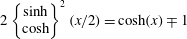 $2\left\{\begin{array}{@{}c@{}}\sinh \\ \cosh \end{array}\right\}^{2}(x/2)=\cosh (x)\mp 1$
, we obtain (Anderson Reference Anderson1989; Yariv Reference Yariv2011)
 $$\begin{eqnarray}\tanh \left(\frac{\unicode[STIX]{x1D711}^{(0)}(\unicode[STIX]{x1D70C},\unicode[STIX]{x1D703})-\unicode[STIX]{x1D6F7}(1,\unicode[STIX]{x1D703})}{4}\right)=\tanh \left(\frac{\unicode[STIX]{x1D701}(\unicode[STIX]{x1D703})}{4}\right)e^{-\sqrt{C_{s}^{\ast }}\unicode[STIX]{x1D70C}},\end{eqnarray}$$
where
 $\unicode[STIX]{x1D701}(\unicode[STIX]{x1D703})=\unicode[STIX]{x1D711}_{s}-\unicode[STIX]{x1D6F7}(1,\unicode[STIX]{x1D703})$
.
B.3 Momentum conservation
Writing the Stokes equations in spherical polar coordinates,
 $$\begin{eqnarray}\displaystyle & \displaystyle \left(\unicode[STIX]{x1D735}\boldsymbol{\cdot }\unicode[STIX]{x1D72B}\right)\boldsymbol{\cdot }\hat{\boldsymbol{e}}_{r}=\unicode[STIX]{x1D6FB}^{2}v_{r}-\frac{2v_{r}}{r^{2}}-\frac{2}{r^{2}\sin \unicode[STIX]{x1D703}}\frac{\unicode[STIX]{x2202}}{\unicode[STIX]{x2202}\unicode[STIX]{x1D703}}\left(\sin \unicode[STIX]{x1D703}\,v_{\unicode[STIX]{x1D703}}\right)-\frac{\unicode[STIX]{x2202}p}{\unicode[STIX]{x2202}r}+\frac{\unicode[STIX]{x2202}\unicode[STIX]{x1D6F7}}{\unicode[STIX]{x2202}r}\unicode[STIX]{x1D6FB}^{2}\unicode[STIX]{x1D6F7}=0, & \displaystyle\end{eqnarray}$$
 $$\begin{eqnarray}\displaystyle & \displaystyle \left(\unicode[STIX]{x1D735}\boldsymbol{\cdot }\unicode[STIX]{x1D72B}\right)\boldsymbol{\cdot }\hat{\boldsymbol{e}}_{\unicode[STIX]{x1D703}}=\unicode[STIX]{x1D6FB}^{2}v_{\unicode[STIX]{x1D703}}-\frac{v_{\unicode[STIX]{x1D703}}}{r^{2}\sin ^{2}\unicode[STIX]{x1D703}}+\frac{2}{r^{2}}\frac{\unicode[STIX]{x2202}v_{r}}{\unicode[STIX]{x2202}\unicode[STIX]{x1D703}}-\frac{1}{r}\frac{\unicode[STIX]{x2202}p}{\unicode[STIX]{x2202}\unicode[STIX]{x1D703}}+\frac{1}{r}\frac{\unicode[STIX]{x2202}\unicode[STIX]{x1D6F7}}{\unicode[STIX]{x2202}\unicode[STIX]{x1D703}}\unicode[STIX]{x1D6FB}^{2}\unicode[STIX]{x1D6F7}=0, & \displaystyle\end{eqnarray}$$
 $$\begin{eqnarray}\displaystyle & \displaystyle \unicode[STIX]{x1D735}\boldsymbol{\cdot }\boldsymbol{v}=\frac{\unicode[STIX]{x2202}v_{r}}{\unicode[STIX]{x2202}r}+\frac{2v_{r}}{r}+\frac{1}{r\sin \unicode[STIX]{x1D703}}\frac{\unicode[STIX]{x2202}}{\unicode[STIX]{x2202}\unicode[STIX]{x1D703}}\left(\sin \unicode[STIX]{x1D703}\,v_{\unicode[STIX]{x1D703}}\right)=0. & \displaystyle\end{eqnarray}$$
To the leading order in the inner expansion (see (B 2)–(B 4)), the static pressure balances the electrostatic stresses normal to the surface (Anderson Reference Anderson1989; Yariv Reference Yariv2011)
 $$\begin{eqnarray}\hat{\boldsymbol{e}}_{\unicode[STIX]{x1D70C}}:\unicode[STIX]{x1D706}^{-3}\left(-\frac{\unicode[STIX]{x2202}{\mathcal{P}}^{(-2)}}{\unicode[STIX]{x2202}\unicode[STIX]{x1D70C}}-\mathop{\sum }_{i}{\mathcal{Z}}_{i}{\mathcal{C}}_{i}^{(0)}\frac{\unicode[STIX]{x2202}\unicode[STIX]{x1D711}^{(0)}}{\unicode[STIX]{x2202}\unicode[STIX]{x1D70C}}\right)+\unicode[STIX]{x1D706}^{-2}\frac{\unicode[STIX]{x2202}^{2}{\mathcal{V}}_{\unicode[STIX]{x1D70C}}^{(0)}}{\unicode[STIX]{x2202}\unicode[STIX]{x1D70C}^{2}}+O\left(\unicode[STIX]{x1D706}^{-1}\right)=0.\end{eqnarray}$$
Note that the expansion for the pressure field begins at
 ${\mathcal{P}}^{(-2)}$
to balance
 $O(\unicode[STIX]{x1D706}^{-2})$
radial electric stresses that cannot be accounted by the viscous stresses (Anderson Reference Anderson1989; Yariv Reference Yariv2011). The viscous stresses balances the static pressure gradient and tangential electric stresses along the surface
 $$\begin{eqnarray}\displaystyle \hat{\boldsymbol{e}}_{\unicode[STIX]{x1D703}}:\unicode[STIX]{x1D706}^{-2}\left(\frac{\unicode[STIX]{x2202}^{2}{\mathcal{V}}_{\unicode[STIX]{x1D703}}^{(0)}}{\unicode[STIX]{x2202}\unicode[STIX]{x1D70C}^{2}}-\frac{\unicode[STIX]{x2202}{\mathcal{P}}^{(-2)}}{\unicode[STIX]{x2202}\unicode[STIX]{x1D703}}-\mathop{\sum }_{i}{\mathcal{Z}}_{i}{\mathcal{C}}_{i}^{(0)}\frac{\unicode[STIX]{x2202}\unicode[STIX]{x1D711}^{(0)}}{\unicode[STIX]{x2202}\unicode[STIX]{x1D703}}\right)+O\left(\unicode[STIX]{x1D706}^{-1}\right)=0, & & \displaystyle\end{eqnarray}$$
with the leading-order incompressibility constraint
 $$\begin{eqnarray}\unicode[STIX]{x1D706}^{-1}\frac{\unicode[STIX]{x2202}{\mathcal{V}}_{\unicode[STIX]{x1D70C}}^{(0)}}{\unicode[STIX]{x2202}\unicode[STIX]{x1D70C}}+O\left(1\right)=0.\end{eqnarray}$$
Therefore, to leading
 $O(\unicode[STIX]{x1D706}^{-3})$
in (B 37), the static pressure balances the radial electrostatic stress
 $$\begin{eqnarray}-\frac{\unicode[STIX]{x2202}{\mathcal{P}}^{(-2)}}{\unicode[STIX]{x2202}\unicode[STIX]{x1D70C}}-\mathop{\sum }_{i}{\mathcal{Z}}_{i}{\mathcal{C}}_{i}^{(0)}\frac{\unicode[STIX]{x2202}\unicode[STIX]{x1D711}^{(0)}}{\unicode[STIX]{x2202}\unicode[STIX]{x1D70C}}=0,\end{eqnarray}$$
which gives the static pressure field
 $$\begin{eqnarray}{\mathcal{P}}^{(-2)}\left(\unicode[STIX]{x1D70C},\unicode[STIX]{x1D703}\right)=2C_{s}^{\ast }(\unicode[STIX]{x1D703})\sinh ^{2}\left(\frac{\unicode[STIX]{x1D711}^{(0)}(\unicode[STIX]{x1D70C},\unicode[STIX]{x1D703})-\unicode[STIX]{x1D6F7}(1,\unicode[STIX]{x1D703})}{2}\right),\end{eqnarray}$$
where matching with the outer solution implies
 ${\mathcal{P}}^{(-2)}(\infty ,\unicode[STIX]{x1D703})=0$
(since the outer field
 $p$
expansion begins at
 $O(1)$
). The next-order
 $O(\unicode[STIX]{x1D706}^{-2})$
in (B 37), momentum balance is
 $$\begin{eqnarray}\frac{\unicode[STIX]{x2202}^{2}{\mathcal{V}}_{\unicode[STIX]{x1D70C}}^{(0)}}{\unicode[STIX]{x2202}\unicode[STIX]{x1D70C}^{2}}=0,\end{eqnarray}$$
where the continuity equation (B 39),
 $\unicode[STIX]{x2202}_{\unicode[STIX]{x1D70C}}{\mathcal{V}}_{\unicode[STIX]{x1D70C}}^{(0)}=0$
(i.e.
 ${\mathcal{V}}_{\unicode[STIX]{x1D70C}}^{(0)}$
is
 $\unicode[STIX]{x1D70C}$
independent), implies
 $$\begin{eqnarray}{\mathcal{V}}_{\unicode[STIX]{x1D70C}}^{(0)}\left(\unicode[STIX]{x1D70C},\unicode[STIX]{x1D703}\right)=\boldsymbol{U}^{e}\boldsymbol{\cdot }\hat{\boldsymbol{e}}_{\unicode[STIX]{x1D70C}}.\end{eqnarray}$$
At
 $O(\unicode[STIX]{x1D706}^{-2})$
in (B 38), viscous stresses balance the tangential pressure gradient
 $\unicode[STIX]{x2202}_{\unicode[STIX]{x1D703}}{\mathcal{P}}^{(-2)}$
and the tangential electrical stress;
 $$\begin{eqnarray}\frac{\unicode[STIX]{x2202}^{2}{\mathcal{V}}_{\unicode[STIX]{x1D703}}^{(0)}}{\unicode[STIX]{x2202}\unicode[STIX]{x1D70C}^{2}}-\frac{\unicode[STIX]{x2202}{\mathcal{P}}^{(-2)}}{\unicode[STIX]{x2202}\unicode[STIX]{x1D703}}-\mathop{\sum }_{i}{\mathcal{Z}}_{i}{\mathcal{C}}_{i}^{(0)}\frac{\unicode[STIX]{x2202}\unicode[STIX]{x1D711}^{(0)}}{\unicode[STIX]{x2202}\unicode[STIX]{x1D703}}=0.\end{eqnarray}$$
Using (B 41) and (B 27), we obtain
 $$\begin{eqnarray}\displaystyle \frac{\unicode[STIX]{x2202}^{2}{\mathcal{V}}_{\unicode[STIX]{x1D703}}^{(0)}}{\unicode[STIX]{x2202}\unicode[STIX]{x1D70C}^{2}} & = & \displaystyle 2\sinh ^{2}\left(2\unicode[STIX]{x1D711}\right)\frac{\unicode[STIX]{x2202}C_{s}^{\ast }}{\unicode[STIX]{x2202}\unicode[STIX]{x1D703}}-2C_{s}^{\ast }\sinh \left(2\unicode[STIX]{x1D711}\right)\cosh \left(2\unicode[STIX]{x1D711}\right)\nonumber\\ \displaystyle & = & \displaystyle \frac{2\tanh \left(2\unicode[STIX]{x1D711}\right)}{1-\tanh ^{2}\left(2\unicode[STIX]{x1D711}\right)}\left[\tanh \left(2\unicode[STIX]{x1D711}\right)\frac{\unicode[STIX]{x2202}C_{s}^{\ast }}{\unicode[STIX]{x2202}\unicode[STIX]{x1D703}}+C_{s}^{\ast }\frac{\unicode[STIX]{x2202}\unicode[STIX]{x1D6F7}}{\unicode[STIX]{x2202}\unicode[STIX]{x1D703}}\right],\end{eqnarray}$$
where
 $4\unicode[STIX]{x1D711}(\unicode[STIX]{x1D70C},\unicode[STIX]{x1D703})=\unicode[STIX]{x1D711}^{(0)}(\unicode[STIX]{x1D70C},\unicode[STIX]{x1D703})-\unicode[STIX]{x1D6F7}(1,\unicode[STIX]{x1D703})$
. Using the identity
 $\tanh (2x)=2\tanh (x)/(1+\tanh ^{2}(x))$
,
 $$\begin{eqnarray}\displaystyle \frac{\unicode[STIX]{x2202}^{2}{\mathcal{V}}_{\unicode[STIX]{x1D703}}^{(0)}}{\unicode[STIX]{x2202}\unicode[STIX]{x1D70C}^{2}}=2\left[\frac{4\tanh ^{2}(\unicode[STIX]{x1D711})\displaystyle \frac{\unicode[STIX]{x2202}C_{s}^{\ast }}{\unicode[STIX]{x2202}\unicode[STIX]{x1D703}}}{\left(1+\tanh (\unicode[STIX]{x1D711})\right)^{2}\left(1-\tanh (\unicode[STIX]{x1D711})\right)^{2}}-\frac{2\tanh (\unicode[STIX]{x1D711})C_{s}^{\ast }\displaystyle \frac{\unicode[STIX]{x2202}\unicode[STIX]{x1D6F7}}{\unicode[STIX]{x2202}\unicode[STIX]{x1D703}}}{\left(1+\tanh (\unicode[STIX]{x1D711})\right)^{2}\left(1-\tanh (\unicode[STIX]{x1D711})\right)^{2}}\right]. & & \displaystyle \nonumber\\ \displaystyle & & \displaystyle\end{eqnarray}$$
It is helpful to write the coefficients of the right-hand side first and second terms as
 $$\begin{eqnarray}\displaystyle \frac{4\tanh ^{2}(\unicode[STIX]{x1D711})}{\left(1+\tanh (\unicode[STIX]{x1D711})\right)^{2}\left(1-\tanh (\unicode[STIX]{x1D711})\right)^{2}} & = & \displaystyle \frac{-1}{\left(1+\tanh (\unicode[STIX]{x1D711})\right)}+\frac{1}{\left(1+\tanh (\unicode[STIX]{x1D711})\right)^{2}}\nonumber\\ \displaystyle & & \displaystyle +\,\frac{-1}{\left(1-\tanh (\unicode[STIX]{x1D711})\right)}+\frac{1}{\left(1-\tanh (\unicode[STIX]{x1D711})\right)^{2}},\end{eqnarray}$$
 $$\begin{eqnarray}\displaystyle \frac{2\tanh (\unicode[STIX]{x1D711})}{\left(1+\tanh (\unicode[STIX]{x1D711})\right)^{2}\left(1-\tanh (\unicode[STIX]{x1D711})\right)^{2}} & = & \displaystyle \frac{1}{\left(1+\tanh (\unicode[STIX]{x1D711})\right)}+\frac{-1}{\left(1+\tanh (\unicode[STIX]{x1D711})\right)^{2}}\nonumber\\ \displaystyle & & \displaystyle +\,\frac{-1}{\left(1-\tanh (\unicode[STIX]{x1D711})\right)}+\frac{1}{\left(1-\tanh (\unicode[STIX]{x1D711})\right)^{2}}.\end{eqnarray}$$
Using (B 33) and integrating once, we obtain
 $$\begin{eqnarray}\displaystyle \frac{\unicode[STIX]{x2202}{\mathcal{V}}_{\unicode[STIX]{x1D703}}^{(0)}}{\unicode[STIX]{x2202}\unicode[STIX]{x1D70C}}=\frac{2}{\sqrt{C_{s}^{\ast }}}\left[\frac{2Q^{2}}{\left(Q^{2}-e^{2\sqrt{C_{s}^{\ast }}\unicode[STIX]{x1D70C}}\right)}\frac{\unicode[STIX]{x2202}{\mathcal{C}}^{\ast }}{\unicode[STIX]{x2202}\unicode[STIX]{x1D703}}-\frac{2Qe^{\sqrt{C_{s}^{\ast }}\unicode[STIX]{x1D70C}}}{\left(Q^{2}-e^{2\sqrt{C_{s}^{\ast }}\unicode[STIX]{x1D70C}}\right)}C_{s}^{\ast }\frac{\unicode[STIX]{x2202}\unicode[STIX]{x1D6F7}}{\unicode[STIX]{x2202}\unicode[STIX]{x1D703}}\right], & & \displaystyle\end{eqnarray}$$
where
 $Q=\tanh (\unicode[STIX]{x1D701}(\unicode[STIX]{x1D703})/4)$
and such that matching with the outer solution imposes
 $\unicode[STIX]{x2202}_{\unicode[STIX]{x1D70C}}{\mathcal{V}}_{\unicode[STIX]{x1D703}}^{(0)}(\infty ,\unicode[STIX]{x1D703})=0$
. In obtaining the above expression, we have used the following integral identities
 $$\begin{eqnarray}\displaystyle & \displaystyle \int \frac{\text{d}\unicode[STIX]{x1D70C}^{\prime }}{1+Qe^{-\sqrt{C_{s}^{\ast }}\unicode[STIX]{x1D70C}^{\prime }}}=\frac{1}{\sqrt{C_{s}^{\ast }}}\ln \left(Q+e^{\sqrt{C_{s}^{\ast }}\unicode[STIX]{x1D70C}}\right)+\text{const.}, & \displaystyle\end{eqnarray}$$
 $$\begin{eqnarray}\displaystyle & \displaystyle \int \frac{\text{d}\unicode[STIX]{x1D70C}^{\prime }}{\left(1+Qe^{-\sqrt{C_{s}^{\ast }}\unicode[STIX]{x1D70C}^{\prime }}\right)^{2}}=\frac{1}{\sqrt{C_{s}^{\ast }}}\frac{Q}{\left(Q+e^{\sqrt{C_{s}^{\ast }}}\right)}+\frac{1}{\sqrt{C_{s}^{\ast }}}\ln \left(Q+e^{\sqrt{C_{s}^{\ast }}\unicode[STIX]{x1D70C}}\right)+\text{const.}, & \displaystyle \nonumber\\ \displaystyle & & \displaystyle\end{eqnarray}$$
 $$\begin{eqnarray}\displaystyle & \displaystyle \int \frac{\text{d}\unicode[STIX]{x1D70C}^{\prime }}{1-Qe^{-\sqrt{C_{s}^{\ast }}\unicode[STIX]{x1D70C}^{\prime }}}=\frac{1}{\sqrt{C_{s}^{\ast }}}\ln \left(e^{\sqrt{C_{s}^{\ast }}\unicode[STIX]{x1D70C}}-Q\right)+\text{const.}, & \displaystyle\end{eqnarray}$$
 $$\begin{eqnarray}\displaystyle & \displaystyle \int \frac{\text{d}\unicode[STIX]{x1D70C}^{\prime }}{\left(1-Qe^{-\sqrt{C_{s}^{\ast }}\unicode[STIX]{x1D70C}^{\prime }}\right)^{2}}=-\frac{1}{\sqrt{C_{s}^{\ast }}}\frac{Q}{\left(Q+e^{\sqrt{C_{s}^{\ast }}}\right)}+\frac{1}{\sqrt{C_{s}^{\ast }}}\ln \left(e^{\sqrt{C_{s}^{\ast }}\unicode[STIX]{x1D70C}}-Q\right)+\text{const.} & \displaystyle \nonumber\\ \displaystyle & & \displaystyle\end{eqnarray}$$
Finally, integrating again,
 $$\begin{eqnarray}\displaystyle {\mathcal{V}}_{\unicode[STIX]{x1D703}}^{(0)}\left(\unicode[STIX]{x1D70C},\unicode[STIX]{x1D703}\right) & = & \displaystyle {\mathcal{V}}_{\unicode[STIX]{x1D703}}^{(0)}(0,\unicode[STIX]{x1D703})+\frac{2}{C_{s}^{\ast }}\frac{\unicode[STIX]{x2202}C_{s}^{\ast }}{\unicode[STIX]{x2202}\unicode[STIX]{x1D703}}\ln \left(\frac{1-Q^{2}e^{-2\unicode[STIX]{x1D70C}\sqrt{C_{s}^{\ast }}}}{1-Q^{2}}\right)\nonumber\\ \displaystyle & & \displaystyle -\,4\frac{\unicode[STIX]{x2202}\unicode[STIX]{x1D6F7}}{\unicode[STIX]{x2202}\unicode[STIX]{x1D703}}\left(\tanh ^{-1}\left(Qe^{-\sqrt{C_{s}^{\ast }}\unicode[STIX]{x1D70C}}\right)-\tanh ^{-1}\left(Q\right)\right).\end{eqnarray}$$
Therefore, in the thin-layer limit
 $\unicode[STIX]{x1D706}\rightarrow 0$
and
 $\unicode[STIX]{x1D70C}\rightarrow \infty$
,
 $$\begin{eqnarray}\lim _{\unicode[STIX]{x1D706}\rightarrow 0;\unicode[STIX]{x1D70C}\rightarrow \infty }{\mathcal{V}}_{\unicode[STIX]{x1D703}}^{(0)}\left(\unicode[STIX]{x1D70C},\unicode[STIX]{x1D703}\right)={\mathcal{V}}_{\unicode[STIX]{x1D703}}^{(0)}(0,\unicode[STIX]{x1D703})+\unicode[STIX]{x1D701}(\unicode[STIX]{x1D703})\frac{\unicode[STIX]{x2202}\unicode[STIX]{x1D6F7}}{\unicode[STIX]{x2202}\unicode[STIX]{x1D703}}-\frac{2}{C_{s}^{\ast }}\frac{\unicode[STIX]{x2202}C_{s}^{\ast }}{\unicode[STIX]{x2202}\unicode[STIX]{x1D703}}\ln \left(1-\tanh ^{2}\left(\frac{\unicode[STIX]{x1D701}(\unicode[STIX]{x1D703})}{4}\right)\right).\end{eqnarray}$$
Finally, matching with the leading-order outer flow field
 $$\begin{eqnarray}\lim _{\unicode[STIX]{x1D706}\rightarrow 0;\unicode[STIX]{x1D70C}\rightarrow \infty }{\mathcal{V}}_{\unicode[STIX]{x1D703}}^{(0)}\left(\unicode[STIX]{x1D70C},\unicode[STIX]{x1D703}\right)=\lim _{r\rightarrow 1,\unicode[STIX]{x1D706}\rightarrow 0}\boldsymbol{v}^{(0)}(r,\unicode[STIX]{x1D703})=\boldsymbol{v}(1,\unicode[STIX]{x1D703}),\end{eqnarray}$$
we obtain the slip velocity boundary condition for the outer flow (Anderson et al. Reference Anderson, Lowell and Prieve1982; Yariv Reference Yariv2011)
 $$\begin{eqnarray}\boldsymbol{v}(1,\unicode[STIX]{x1D703})=\boldsymbol{U}^{e}+\left[\unicode[STIX]{x1D701}(\unicode[STIX]{x1D703})\frac{\unicode[STIX]{x2202}\unicode[STIX]{x1D6F7}}{\unicode[STIX]{x2202}\unicode[STIX]{x1D703}}+4\frac{\unicode[STIX]{x2202}\ln C_{s}^{\ast }}{\unicode[STIX]{x2202}\unicode[STIX]{x1D703}}\ln \cosh \left(\frac{\unicode[STIX]{x1D701}(\unicode[STIX]{x1D703})}{4}\right)\right]\hat{\boldsymbol{e}}_{\unicode[STIX]{x1D703}}.\end{eqnarray}$$