


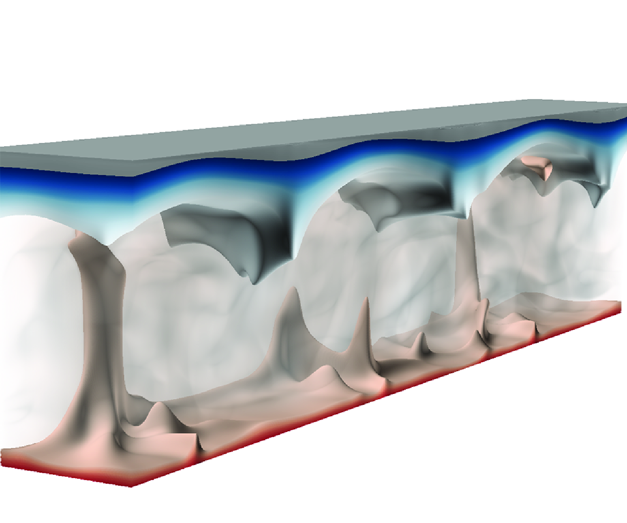

1. Introduction
Icebergs released from the Greenland and Antarctic ice sheets are one of the dominant sources of freshwater discharged into the oceans (Silva, Bigg & Nicholls Reference Silva, Bigg and Nicholls2006; England, Wagner & Eisenman Reference England, Wagner and Eisenman2020). Such a process accounts for
 $45\,\%$
of Antarctic freshwater loss (Rignot et al. Reference Rignot, Jacobs, Mouginot and Scheuchl2013) and dominates the freshwater production in Greenland fjords (Enderlin et al. Reference Enderlin, Hamilton and Sutherland2016). The melting of icebergs is one of the key factors for the changing of environmental conditions and actively participates in many geophysical processes (Bintanja & de Wal Reference Bintanja and van de Wal2008; Notz Reference Notz2009; Shepherd et al. Reference Shepherd, Hubbard, Nienow, King, McMillan and Joughin2009; Tietsche et al. Reference Tietsche, Notz, Jungclaus and Marotzke2011; Hanna et al. Reference Hanna2013), thus being highly relevant to the global climate evolution (Clark, Alley & Pollard Reference Clark, Alley and Pollard1999; Golledge et al. Reference Golledge, Keller, Gomez, Naughten, Bernales, Trusel and Edwards2019). Iceberg melting is usually coupled with the convective flows in the surrounding seawater fluid, and the plumes within the convection zone facilitate the transport of momentum, heat and mass, such as nutrients, in the upper ocean (Bhatia et al. Reference Bhatia, Kujawinski, Das, Breier, Henderson and Charette2013; Smith et al. Reference Smith, Sherman, Shaw and Sprintall2013; Bigg Reference Bigg2016; Duprat, BIgg & Wilton Reference Duprat, Bigg and Wilton2016). It is then of great importance to accurately quantify the melting rate of glacial ice in the ocean, which has attracted numerous interest in recent years (Edwards et al. Reference Edwards2021; Cenedese & Straneo Reference Cenedese and Straneo2023; Du, Calzavarini & Sun Reference Du, Calzavarini and Sun2024; Rosevear et al. Reference Rosevear, Gayen, Vreugdenhil and Galton-Fenzi2025).
To understand the underlying dynamics of ice melting, different flow configurations and factors have been investigated. For a comprehensive review, please refer to the recent work of Du et al. (Reference Du, Calzavarini and Sun2024). For single component buoyant fluid, many studies have revealed that the convection motions have profound influences on the ice–fluid interface morphology and melting process. The convection motions induced by melting share a great resemblance with the traditional Rayleigh–Bénard (RB) convection, such as the scaling of global quantities (Esfahani et al. Reference Esfahani, Hirata, Berti and Calzavarini2018). The size of convection cells can strongly alter the topography of the ice surface during the melting (Favier, Purseed & Duchemin Reference Favier, Purseed and Duchemin2019). Detailed studies at larger Rayleigh numbers further suggests that the interface roughness can be spontaneously generated by convection motions, and the relation between the roughness amplitude and the mean height of the fluid layer can be explained by scaling laws (Yang et al. Reference Yang, Howland, Liu, Verzicco and Lohse2023b ). In reality, the convection motions can be modulated by external shear and the melting process is altered simultaneously, which has also been extensively investigated in recent years (Toppaladoddi & Wettlaufer Reference Toppaladoddi and Wettlaufer2019; Couston et al. Reference Couston, Hester, Favier, Taylor, Holland and Jenkins2021; Hester et al. Reference Hester, McConnochie, Cenedese, Couston and Vasil2021; Toppaladoddi Reference Toppaladoddi2021; Lu et al. Reference Lu, Zhang, Luo, Wu and Yi2022). Other relevant effects include the aspect ratio of the ice block and the ambient water velocity; see, e.g. Hester et al. (Reference Hester, McConnochie, Cenedese, Couston and Vasil2021).
When solid ice melts in the seawater, the flow system is much more complex compared with that in pure water. The presence of salinity significantly alters the melting process (Huppert & Turner Reference Huppert and Turner1978, Reference Huppert and Turner1980). On the one hand, the melting temperature depends on the actual salinity at the ice–seawater interface. On the other hand, the density of seawater is determined by both temperature and salinity. Therefore, the buoyancy-driven motions generated during the melting is actually double diffusive convection (Kang et al. Reference Kang, Mittal, Bire, Campin and Marshall2022). Large-scale large-eddy simulations indicate that double diffusive convection controls the basal melting of ice and the vertical mixing beneath (Rosevear, Gayen & Galton-Fenzi Reference Rosevear, Gayen and Galton-Fenzi2021). Detailed dynamics at the melting ice surface have also been studied extensively by using a fixed phase interface for basal melting (Vreugdenhil & Taylor Reference Vreugdenhil and Taylor2019; Middleton et al. Reference Middleton, Vreugdenhil, Holland and Taylor2021) and front melting (Wells & Worster Reference Wells and Worster2011; Gayen, Griffiths & Kerr Reference Gayen, Griffiths and Kerr2016; Mondal et al. Reference Mondal, Gayen, Griffiths and Kerr2019). For basal melting, the interplay between the turbulence and double diffusive convection strongly affects the overall flow morphology (Vreugdenhil & Taylor Reference Vreugdenhil and Taylor2019; Middleton et al. Reference Middleton, Vreugdenhil, Holland and Taylor2021). As salinity concentrations increase, diverse flow motions may emerge (Xue, Zhang & Ni Reference Xue, Zhang and Ni2024). For a time-evolving phase interface, the topographic features of the ice surface are shaped by the double diffusive motions nearby, such as the ‘sharkskin’ texture for melting from above (Sugawara et al. Reference Sugawara, Ishikura and Beer2005, Reference Sugawara, Tamura, Satoh, Komatsu, Tago and Beer2007) and the ice scalloping at a vertical front (Wilson et al. Reference Wilson, Vreugdenhil, Gayen and Hester2023). For the vertical ice front, the interplay between the thermally induced stratification and the salinity induced stratification control the flow strength near the ice front and, therefore, the front shape and the melting rate (Yang et al. Reference Yang, Howland, Liu, Verzicco and Lohse2023a ).
Another important factor that influences ice melting in seawater is the nonlinear equation of state of seawater. Specifically, the density of seawater varies non-monotonically with temperature and salinity. The density can reach its maximum within the flow domain, instead of at the top boundary as in a traditional RB configuration. It has long been known that the existence of maximal density inside the flow domain has a profound impact on the phase-changing dynamics of seawater (Dumore, Merk & Prins Reference Dumore, Merk and Prins1953; Carey, Gebhart & Mollendorf Reference Carey, Gebhart and Mollendorf1980; Carey & Gebhart Reference Carey and Gebhart1981). Even for ice melting in fresh water, experiments and numerical simulations have revealed that very rich dynamics and flow morphology emerge under different thermal conditions. The shape of a vertical ice front depends on the vertical convection inside the water region, which is strongly affected by density inversion (Wang et al. Reference Wang, Jiang, Du and Sun2021d ; Yang et al. Reference Yang, Chong, Liu, Verzicco and Lohse2022, Reference Yang, Howland, Liu, Verzicco and Lohse2023a ). While in the RB-like configuration with a vertical temperature gradient, density inversion induces the emergence of a stably stratified fluid layer (Wang et al. Reference Wang, Calzavarini, Sun and Toschi2021c ; Du et al. Reference Du, Wang, Jiang, Calzavarini and Sun2023). In flipped RB systems, it significantly affects the phase-change dynamics and ice front morphology (Townsend Reference Townsend1964; Tsai, Yang & Hwang Reference Tsai, Yang and Hwang1998; Couston Reference Couston2021; Wang et al. Reference Wang, Jiang, Du and Sun2021d ). Additionally, density inversion can induce multi-equilibrium states depending on initial conditions (Wang et al. Reference Wang, Calzavarini and Sun2021b ). These effects, including the formation of scallop patterns on ice fronts (Weady et al. Reference Weady, Tong, Zidovska and Ristroph2022), highlight the complex interplay between density inversion and ice melting dynamics.
Therefore, the melting of solid ice in seawater involves the heat transfer inside ice, the phase-changing process at the interface, the heat and mass exchange between ice and seawater, and the double diffusive convection inside the liquid. Also the nonlinear equation of state should be considered for seawater in order to include the density inversion effect. It should be pointed out that Xue et al. (Reference Xue, Zhang and Ni2024) has investigated the interaction between the double diffusive convection and the pure ice melting, where only a linear equation of state was used. However, the novelty of the current study is twofold. First, a nonlinear equation of state will be employed and its influence on the flow dynamics will be examined for the parameters relevant to the ocean. Second, a theoretical model will be constructed to explain the regime transition revealed by our numerical simulations. For these purposes, we develop an efficient numerical solver that can simultaneously simulate the phase-changing process by using an enthalpy-based method and the temporal evolution of a shape-changing ice surface by using an immersed-boundary method. Systematic direct numerical simulations (DNS) will then be conducted.
The paper is structured as follows. In
 $\S$
2 we describe the theoretical formulation and numerical methods. The time evolution of the flow morphology and melting process is discussed in
 $\S$
3, along with the introduction of different flow regimes. In
 $\S$
4 we develop theoretical models for the global transport properties, the properties at the ice–seawater interface front and the critical parameters for the transition between different flow regimes. The effects of density inversion are discussed in
 $\S$
5. Finally, conclusions are given in
 $\S$
6.
2. Governing equations and numerical methods
To study the melting of pure ice in seawater, a two-layer flow system is employed as shown in figure 1. Initially, a layer of ice lies above a layer of warm seawater. The total height of the domain is
 $H$
. The initial height of the seawater layer is
 $Hh_0$
, here
 $h_0$
represents the initial dimensionless height of the liquid layer. Denote the temperature and salinity of seawater by
 $T$
and
 $S$
, respectively. The initial temperature of ice is uniform and set to
 $T_0=0\,^{\,\circ} \textrm{C}$
. To facilitate the ice melting, the bottom boundary of the domain has a fixed temperature
 $T_b$
that is higher than
 $T_0$
, i.e.
 $T_b\gt T_0$
. The salinity at the bottom boundary remains constant at
 $S_b$
. Since most of the heat transported from seawater to ice is consumed by the phase changing at the ice–water interface, the heat loss from the top boundary is negligible, and the adiabatic condition is used. The adiabatic condition naturally holds for the salinity field at the top boundary as well. Under these conditions, the ice layer will completely melt at the final state.
Schematic illustration of the melting problem involving a binary fluid. (a) The initial configuration for the simulations. (b) The evolving stage of the system.

For fresh water, the density is maximal at
 $T^f_m=4^{\,\circ} \textrm{C}$
, while for seawater, the density is affected by many factors and the equation of state is strongly nonlinear. The full nonlinear equation of state, for example, TEOS-10 equation of state (IOC et al. 2010), takes a very complex form. Here, to make the analyses more systematic and manageable, instead of the fully nonlinear equation, we use a simplified equation of state that keeps the essential nonlinearity effect as
 \begin{equation} \rho = \rho _0+\rho '=\rho _0 -\frac {C_b}{2}{\left (T-T_m\right )}^2+b_{0}S. \end{equation}
Here
 $\rho _0$
is a reference density and
 $\rho '=\rho -\rho _0$
is the density anomaly with respect to
 $\rho _0$
. The density inversion temperature
 $T_m$
is dependent on local salinity
 $S$
according to the relation
 $T_m=T^f_m+C_sS$
. Other coefficients in the equation of state are set as
 $C_b=0.011\,\textrm{kg}\,\textrm{m}^{-3}\,\textrm{K}^{-2}$
,
 $b_0=0.77\,\textrm{kg}\,\textrm{m}^{-3}\,\textrm{psu}^{-1}$
and
 $C_s=-0.25\,\textrm{K}\,\textrm{psu}^{-1}$
. Such a choice is very common in the studies of ice melting in seawater, see, e.g. Roquet et al. (Reference Roquet, Madec, Brodeau and Nycander2015) and Yang et al. (Reference Yang, Howland, Liu, Verzicco and Lohse2023a
).
Denote the vertical coordinate by
 $z$
and the two horizontal coordinates by
 $x$
and
 $y$
, respectively. Under the Oberbeck–Boussinesq approximation and by using the equation of state (2.1), the incompressible flow and the dynamics of temperature and salinity within the seawater layer can be described by the following equations:
 \begin{align}&\qquad\qquad\qquad\qquad\qquad\qquad\quad\,\, \nabla \cdot \mathbf{U} = 0, \end{align}
 \begin{align}& \partial _{t}\mathbf{U}+\mathbf{U}\cdot \nabla \mathbf{U} = -\frac {\nabla {P}}{\rho _0}+\nu \nabla ^{2}\mathbf{U} +\frac {g}{\rho _0}\left [\frac {C_b}{2}{\left (T-T_m\right )}^2-b_{0}S\right ]\mathbf{e}_z +\mathbf{F}_{\textit{IBM}}, \end{align}
 \begin{align}&\qquad\qquad\qquad\qquad\quad\qquad \partial _{t}T+\mathbf{U}\cdot \nabla T =\kappa _T\nabla ^{2}T, \end{align}
 \begin{align}&\qquad\qquad\qquad\qquad\qquad\quad\, \partial _{t}S+\mathbf{U}\cdot \nabla S =\kappa _S\nabla ^{2}S. \end{align}
Here,
 $\mathbf{U}$
is velocity,
 $P$
is pressure,
 $g$
is gravitational acceleration,
 $\nu$
is kinetic viscosity,
 $\kappa _T$
and
 $\kappa _S$
are the molecular diffusivities of temperature and salinity, respectively.
 $\mathbf{e}_z$
is the unit vector along the vertical
 $z$
direction;
 $\mathbf{F}_{\textit{IBM}}$
is the virtual force introduced by the immersed boundary method (IBM) at the ice–seawater interface, its detailed form will be discussed later with the numerical methods. In (2.2) all the flow variables represented by the capital letters are in their dimensional form.
For the pure ice layer, only the diffusion equation is solved for temperature as
 \begin{equation} \partial _{t}T =\kappa _i\nabla ^{2}T, \end{equation}
where
 $\kappa _i$
is the thermal diffusivity of ice. Both velocity and salinity are zero within the ice layer. In order to write the temperature equations for seawater and ice in a unified form, as proposed by Esfahani et al. (Reference Esfahani, Hirata, Berti and Calzavarini2018), a phase variable
 $\phi$
is introduced and defined as the volume fraction of seawater. Within the seawater layer
 $\phi =1$
and within the ice layer
 $\phi =0$
. At the interface,
 $\phi$
takes a value between
 $0$
and
 $1$
. In our numerical simulations,
 $\phi$
equals the volume fraction of seawater within the Eulerian mesh cell if the cell intersects the ice–seawater interface. Then, for the whole domain, the temperature equation reads
 \begin{equation} \alpha _c\partial _{t}T+\mathbf{U}\cdot \nabla T = \nabla \cdot \left (\alpha _k\kappa _T\nabla T\right ) -\frac {\mathcal{L}}{c_p}\partial _{t}\phi , \end{equation}
with
 \begin{equation} \alpha _k = \phi + \frac {k_i}{k_w}\left (1-\phi \right ), \qquad \alpha _c = \phi + \frac {c_i}{c_p}\left (1-\phi \right ). \end{equation}
Here
 $\mathcal{L}$
is the latent heat,
 $k_i=\kappa _i c_i$
and
 $k_w=\kappa _T c_p$
are the thermal conductivities of ice and seawater,
 $c_i$
and
 $c_p$
are the heat capacity per unit volume of ice and seawater, respectively. Note that with the phase variable
 $\phi$
the salinity equation can be written for the whole domain as
 \begin{equation} \partial _{t}S+\mathbf{U}\cdot \nabla S =\nabla \cdot \left (\phi \kappa _S\nabla S\right ). \end{equation}
Since in the ice layer both
 $\mathbf{U}$
and
 $\phi$
are equal to zero, the above equation is equivalent to
 $S\equiv 0$
within the ice layer as the initial value is set to zero. Additionally, we denote the quantities associated with the interface by the subscript
 $\Gamma$
, according to the liquidus relation for a binary melt, at the ice–seawater interface, the local temperature
 $T_\Gamma$
depends on the local salinity
 $S_\Gamma$
,
 \begin{equation} T_\Gamma + \lambda S_\Gamma = T_0, \end{equation}
in which
 $\lambda =5.71\times 10^{-2}\,^{\,\circ} \textrm{C}$
stands for the liquidus slope of the temperature–salinity binary fluid. The boundary conditions at the top and bottom boundaries of the domain are
 \begin{align} U_x = U_y = U_z = 0,\quad T=T_b,\quad S=S_b, \quad \mbox{at } z &= 0,\\[-10pt]\nonumber \end{align}
 \begin{align} U_x = U_y = U_z = 0,\quad \partial _z T = \partial _z S = 0, \quad \mbox{at } z & = H. \\[12pt] \nonumber \end{align}
Namely, the non-slip condition is used for velocity, while both temperature and salinity are kept constant at the bottom boundary and adiabatic at the top boundary, respectively.
The above governing equations and boundary conditions are non-dimensionalised by using the domain height
 $H$
, the initial temperature difference across the seawater layer
 $\varDelta _{T0}=T_b-T_0$
, the salinity at the bottom boundary
 $S_b$
, the free-fall velocity
 $U_f=\sqrt {gC_b\varDelta _{T0}^2 H/(2\rho _0)}$
and the time scale
 $H/U_f$
. The non-dimensional equations read
 \begin{align}&\qquad\qquad\qquad\qquad\quad\qquad \nabla \cdot \mathbf{u} = 0, \end{align}
 \begin{align}& \partial _{t}\mathbf{u} +\mathbf{u}\cdot \nabla {\mathbf{u}} = -\nabla {p} +\frac {\sqrt {Pr}}{\sqrt {Ra}}\nabla ^{2}\mathbf{u} +\big[{\left (\theta -\theta _m\right )}^2 -\Lambda s \big]\mathbf{e}_z +\mathbf{f}_{\textit{IBM}}, \end{align}
 \begin{align}&\qquad\qquad \alpha _c\partial _{t}{\theta } +\mathbf{u}\cdot \nabla {\theta } = \frac {1}{\sqrt {Pr Ra}}\nabla \cdot \left (\alpha _k \nabla \theta \right )-St\partial _{t}\phi , \end{align}
 \begin{align}&\qquad\qquad\qquad \partial _{t}s +\mathbf{u}\cdot \nabla s = \frac {1}{\sqrt {PrRa}Le}\nabla \cdot \left (\phi \nabla s\right ), \end{align}
 \begin{align}&\qquad\qquad\qquad\qquad\quad\quad \theta _\Gamma + \alpha _\lambda s_\Gamma = \theta _0. \end{align}
Here
 $\mathbf{u}$
and
 $p$
are the non-dimensional velocity and pressure,
 $\theta =(T-T_0)/\varDelta _{T0}$
is the non-dimensional temperature and
 $s=S/S_b$
is the non-dimensional salinity. In (2.9e
),
 $\theta _\Gamma$
and
 $s_\Gamma$
are the non-dimensional interface temperature and salinity, and
 $\alpha _\lambda =\lambda C_b\varDelta _{T0}\Lambda /2b_0$
denotes the non-dimensional liquidus slope. It should also be mentioned that the kinetic and capillary undercooling effects are neglected in the present study, as done in previous works (e.g. Favier et al. Reference Favier, Purseed and Duchemin2019).
The system is then controlled by the Prandtl number, Lewis number, Rayleigh number, density ratio, and the Stefan number, which are respectively defined as
 \begin{equation} Pr = \frac {\nu }{\kappa _T}, \quad Le = \frac {\kappa _T}{\kappa _S}, \quad Ra = \frac {g C_b \varDelta _{T0}^2 H^3}{2\rho _0\kappa _T\nu }, \quad \Lambda = \frac {2b_{0}S_b}{C_b\varDelta _{T0}^2}, \quad St = \frac {\mathcal{L}}{c_p\varDelta _{T0}}. \end{equation}
Other commonly used parameters can be calculated from the above parameters, such as the Schmidt number
 $Sc=Le Pr$
and the salinity Rayleigh number
 $Ra_S=\Lambda Le Ra$
. The non-dimensional density inversion temperature
 $\theta _m$
can be readily obtained by
 \begin{align} \theta _m = \frac {T_m^f-T_0}{\varDelta _{T0}} + C_s\frac {S_b}{\varDelta _{T0}}s. \end{align}
Throughout this study, we set
 $k_i/k_w=2.76$
,
 $c_i/c_p=0.51$
and
 $\alpha _\lambda =4.1\times 10^{-3}\Lambda$
, which are based on field observations (Jenkins, Nicholls & Corr Reference Jenkins, Nicholls and Corr2010; Jenkins Reference Jenkins2011; Hester et al. Reference Hester, McConnochie, Cenedese, Couston and Vasil2021). The Prandtl number is taken as the typical value in the polar oceans, i.e.
 $Pr=10$
. The realistic Schmidt number of salinity is about
 $Sc=1000$
, or corresponding
 $Le=100$
, which poses a severe restriction on the mesh size. Moreover, as will be shown later, the melting process usually is a very slow process. Therefore, to make the DNS simulations feasible, we choose a smaller Lewis number
 $Le=10$
. It has been shown that cases with
 $Le=10$
are capable of investigating the double diffusive effects (Hester et al. Reference Hester, McConnochie, Cenedese, Couston and Vasil2021).
We also fix the temperature difference at
 $\varDelta _{T0}=10\,^{\,\circ} \textrm{C}$
, which gives a Stefan number at
 $St=8.4$
by using the actual values of
 $\mathcal{L}$
and
 $c_p$
. This temperature difference may be larger than the typical values found in the ocean. There are several reasons to use a large temperature difference. First, we want to accelerate the melting process, otherwise the simulations would take too much time to finish. Second, a temperature difference larger than
 $T_m^f$
will ensure that density inversion still happens at small
 $S_b$
. Finally, using a large temperature difference ensures that freezing cannot happen during simulations. Note that the freezing of seawater results in mushy ice instead of solid ice that cannot be dealt with using the current numerical method. Nevertheless, a smaller temperature difference or larger Stefan number only results in much slower melting while the melting dynamics should remain similar. Since the temperature difference is fixed, a different Rayleigh number corresponds to different domain heights.
The Rayleigh number and density ratio are then systematically varied to cover a wide range of parameters. Specifically, the Rayleigh number lies in
 $10^6\leqslant Ra\leqslant 10^9$
and the density ratio in
 $1\leqslant \Lambda \leqslant 50$
. The explored parameters are presented in figure 2. For the temperature difference
 $\varDelta _{T0}=10^{\,\circ} \textrm{C}$
, the density ratio
 $\Lambda =50$
corresponds to the typical oceanic salinity of
 $S_b=35\,\textrm{psu}$
. For smaller temperature differences, the density ratio can be much larger. It may be argued that the current density ratio is too small. For example, when
 $\varDelta _{T0}=2\,^{\,\circ} \textrm{C}$
and
 $S_b=35\,\textrm{psu}$
, the density ratio
 $\Lambda$
will be over
 $1000$
. In reality, fresh water is constantly released into the surrounding seawater as ice melts, and local salinity decreases. The local density ratio also decreases. Moreover, as will be demonstrated later, the flow at
 $\Lambda =50$
will eventually enter the pure diffusion state, and a higher density ratio should lead to the same state. Therefore, the current range of density ratio covers all the relevant flow dynamics.
The parameter space explored in the current simulations. The blue circles mark the cases in the convection-diminishing regime and the red circles mark those in the convection-growing regime. The black dashed line marks the critical density ratio.

For all simulations, a flat ice–seawater interface is initially located at a height
 $h_0$
. We used uniform initial distributions of temperature and salinity in the water and ice layers:
 \begin{align} \theta =\left \{ \begin{aligned} &1, &z&\lt h_0, \\ &0, &z&\geqslant h_0, \end{aligned}\right .\qquad s =\left \{ \begin{aligned} &1, &z&\lt h_0, \\ &0, &z&\geqslant h_0. \end{aligned}\right . \end{align}
To accelerate flow evolution, in all simulations a random perturbation with a magnitude of
 $10^{-3}$
is introduced in the initial fields. Then the ice layer gradually melts due to heating from the bottom. The initial height of the ice front is chosen so that
 $h^3_0=0.1H^3$
and the effective Rayleigh number of the seawater layer is
 $Ra^0_{eff}=0.1Ra$
, i.e. one order of magnitude lower than the total Rayleigh number. Denote the average height of the ice–seawater interface by
 $h_\Gamma$
, which increases during ice melting. The simulations will stop when
 $h_\Gamma =0.9H$
. It should be pointed out that
 $10^5\leqslant Ra_{eff}^0\leqslant 10^8$
corresponds to an initial seawater layer with a height of
 $0.01{-}0.3\,\textrm{m}$
. For pure ice melting in seawater, the thermal and salinity diffusive boundary layers adjacent to the ice fronts have a thickness of about
 $O(1{-}10)\,\textrm{mm}$
, and the mixed layer that is affected by the melting process has a typical depth of
 $O(10{-}100)\,\textrm{mm}$
(Rosevear et al. Reference Rosevear, Gayen, Vreugdenhil and Galton-Fenzi2025). The dimensional height of the current simulation is thicker than the diffusive layer but well embedded inside the mixed layer. Uniform distributions of temperature and salinity are a reasonable choice for the initial condition.
The governing equation (2.9) is numerically solved using our in-house code that employs the second-order finite difference scheme and a fractional time-step method, along with the multiple resolution technique (Ostilla-Mónico et al. Reference Ostilla-Monico, Yang, van der Poel, Lohse and Verzicco2015). Specifically, a Runge–Kutta type of scheme is used for temporal integration, where the nonlinear terms are handled by the explicit Adams–Bashforth scheme and the diffusion terms by the implicit Crank–Nicholson scheme. The velocity and temperature fields are solved on a base mesh, whereas the salinity field, which has a smaller diffusivity, is solved on a refined mesh. Various computational methods have been developed for problems where fluid dynamics is coupled to the process of the ice–seawater phase change. In the present work, the velocity boundary condition at the ice–seawater interface is dealt with in the IBM, and the iterative enthalpy-based method is utilised to simulate the melting process in the multiple component fluid. In our main investigation, simulations are run in two dimensions in order to cover a wide range of control parameters, and the numerical details are summarised in table 1. The horizontal width of the domain is set to
 $L_x=4H$
. The aspect ratio should be large enough to ensure that the periodic boundary condition is applicable. Our choice of aspect ratio is either similar to or larger than that in previous studies (e.g. Esfahani et al. Reference Esfahani, Hirata, Berti and Calzavarini2018; Hester et al. Reference Hester, McConnochie, Cenedese, Couston and Vasil2021; Yang et al. Reference Yang, Howland, Liu, Verzicco and Lohse2023b
; Xue et al. Reference Xue, Zhang and Ni2024). Further details in the numerical methods and several validations are provided in Appendix A. In Appendices B and C we also provided, for limited cases, the comparison between the two-dimensional (2-D) and three-dimensional (3-D) results and the comparison between
 $Le=10$
and
 $Le=100$
, respectively, and no fundamental differences are observed.
Summary of the control parameters and the numerical set-up for 2-D cases. The columns, from left to right, detail the initial Rayleigh number, Rayleigh number, density ratio, Lewis number, the base resolutions and the refinement factors in the
 $x$
and
 $z$
directions, respectively, and the total simulation time.

3. Evolution of flow morphology
Given the initial set-up in the current system, i.e. a layer of ice above a layer of seawater with uniform temperature and salinity, convection motions start from the interface due to the local unstable temperature difference
 $T_0\lt T_b$
. Then as the ice melts, the salinity within the adjacent seawater decreases and a stable salinity gradient grows. The unstable temperature gradient and stable salinity gradient combined drive double diffusive convection in the seawater layer. The flow morphology depends on the density ratio
 $\Lambda$
, which is the ratio between the strength of the temperature gradient and that of the salinity gradient. As a first illustration of such a process, figure 3 shows the temporal evolution of the root-mean-square (r.m.s.) of velocity
 $u_{rms}$
for fixed
 $Ra=10^9$
(
 $Ra_{eff}^0=10^8$
),
 $Le=10$
and increasing
 $\Lambda$
. Initially,
 $u_{rms}$
decreases with time for all cases due to the development of a stable salinity gradient, which is related to the initial condition. When roughly
 $t\gt 500$
,
 $u_{rms}$
exhibits totally different behaviours for the cases with different
 $\Lambda$
. Generally, for small
 $\Lambda$
, flow motions become stronger as the ice melts. Conversely, flow motions becomes weaker with time for larger
 $\Lambda$
. For the large values
 $\Lambda =10$
and
 $\Lambda =20$
, all flow motions disappear within the simulation time period. These different long-term behaviours of
 $u_{rms}$
are caused by different flow morphologies. Based on the numerical results, two different regimes can be identified: the convection-growing regime for small density ratios and the convection-diminishing regime for large density ratios.
The time history of the r.m.s. velocity for cases with fixed
 $Ra=10^9$
and different density ratios.

Characteristics of the convection-growing regime at the parameter settings of
 $(Ra,\Lambda )=(10^9,1)$
. Snapshots of the temperature field (a), the salinity field (b) and the solid–liquid interfaces (white solid lines) at different times (
 $t=100,1000,10\,000$
).

When
 $\Lambda$
is small, the solute-stabilising effect is rather weak, and the flow evolution is dominated by the temperature-destabilising effect. A typical temporal evolution of such a case is illustrated in figure 4 for
 $Ra=10^9$
,
 $Le=10$
and
 $\Lambda =1$
. A series of flow fields at different times are shown for both temperature and salinity. The seawater layer consists of convection rolls that extend from the bottom boundary to the ice–seawater interface all along. It is clear that convection motions emerge first at the interface and take the form of isolated plumes. Note the salinity plumes are much thinner compared with the thermal ones, due to the smaller diffusivity of salinity. These plumes grow downward and drive the large convection rolls. The ice–seawater interface, as indicated by the thick white lines, retreats towards the top boundary as ice melts. The shape of the interface cannot remain flat due to the presence of the large rolls inside the seawater layer. For this case, the density ratio
 $\Lambda =1$
is too small for the salinity gradient to have noticeable effects, and the flow system is very similar to that observed for the iceberg melting in fresh water that corresponds to
 $\Lambda =0$
(Hester et al. Reference Hester, McConnochie, Cenedese, Couston and Vasil2021). If we further increase
 $\Lambda$
to a higher value, e.g. at
 $(Ra,\Lambda )=(10^9,4)$
as displayed in figure 5, we find that an upper stably stratified layer in the liquid forms due to the solute-stabilising effect. The convection rolls are hardly able to penetrate the stably stratified layer, which makes the ice–seawater interface more flat. These distinct scenarios imply that the flow structures for
 $\Lambda =1$
and
 $4$
are not identical, even though both belong to the diffusion regime. In either case, the convection layer grows in height. Therefore, we refer to this type of flow morphology as the convection-growing regime.
Characteristics of the convection-growing regime at the parameter settings of
 $(Ra,\Lambda )=(10^9,4)$
. Snapshots of the temperature field (a), the salinity field (b) and the solid–liquid interfaces (white solid lines) at different times (
 $t=100,1000,10\,000,49\,600$
).

Figure 6 displays the evolution of horizontally averaged scalar profiles for the same case shown in figure 4, where
 $\tilde {\xi }(z,t)=({1}/{L})\int _{0}^{L}\xi (x,z,t)\,{\textrm d}x$
with
 $\xi =\theta ,\,s,\,\rho$
representing the averaged scalars at a given dimensionless height
 $z$
and time
 $t$
. The colour changes from red to blue as the time evolves. The profiles of temperature and salinity within the seawater layer are very similar to that of traditional RB convection, indicating a nearly homogeneous bulk bounded by two thin boundary layers at the bottom boundary and interface. For this case, the mean temperature of the homogeneous bulk first decreases and then stops at a constant about
 $0.6$
, as explained in Wang, Calzavarini & Sun (Reference Wang, Reiter, Lohse and Shishkina2021a
). The heat transfer through the seawater layer from the bottom boundary is consumed by the phase-changing process and heating the newly formed water layer. When the two balance each other, the bulk temperature does not change with time anymore. Meanwhile, the mean salinity of the bulk decreases over time. Figure 6 also plots the horizontally averaged profiles of density anomaly
 $\rho ' = \Lambda s - (\theta -\theta _m)^2$
, as shown in panel (c). The density anomaly profiles also have a nearly homogeneous bulk with the mean value decreasing with time. Within a thin layer near the interface, an unstable stratification appears at the early time but becomes very weak as the flow develops, similar to the flow structure of pure water taking into account the density inversion effect. Figure 7 illustrates the time evolution of horizontally averaged scalar profiles at
 $(Ra,Le,\Lambda )=(10^9,10,4)$
. For this case, the height of the convection layer grows with time. In the diffusive layer above, both the temperature and salinity have a linear profile from the upper edge of the homogeneous layer to the ice–seawater interface. The height of this diffusive layer increases as the ice melts. The density also has a linear profile in this diffusive layer, which is a stably stratified layer due to the temperature and salinity distribution. As the ice melts, the density gradient becomes smaller and the stabilising effect weakens.
The left panels show the time evolution of the horizontally averaged profiles of (a) temperature
 $\theta$
, (b) salinity
 $s$
and (c) density anomaly for the case with
 $(Ra,\Lambda )=(10^9,1)$
. The right panels display the instantaneous vertical profiles of (d) temperature
 $\theta$
, (e) salinity
 $s$
and (f) density anomaly at time
 $t=100,1000,10\,000$
.

The left panels show the time evolution of the horizontally averaged profiles of (a) temperature
 $\theta$
, (b) salinity
 $s$
and (c) density anomaly for the case with
 $(Ra,\Lambda )=(10^9,4)$
. The right panels display the instantaneous vertical profiles of (d) temperature
 $\theta$
, (e) salinity
 $s$
and (f) density anomaly at time
 $t=100,1000,10\,000,49\,600$
.

For a larger density ratio
 $\Lambda$
, the flow evolution takes a different form, which is illustrated by the snapshots of flow field and the scalar profiles shown in figures 8 and 9 for the case with
 $Ra=10^9$
,
 $Le=10$
and
 $\Lambda =10$
. It is evident that although convection rolls are still observable at
 $t=10\,000$
, their strength diminishes and is fully suppressed by
 $t=68\,000$
. Initially, there is also an unstably stratified layer that appears in the whole fluid domain, with a uniform density distribution. However, due to the dominant salinity stabilising effect, as the ice block melts, the fresh fluid forms a stably stratified layer that develops downwards, compressing the convection stratification. The convection rolls are unable to penetrate the stably stratified layer, consequently the solute-stabilising effect gradually dominates over the temperature-destabilising effect, and ultimately, the fluid becomes almost static, with heat and salt transported only in a diffusive manner.
Time evolution of the temperature (a) and salinity (b) fields for the transition case with
 $(Ra,Le,\Lambda )=(10^9,10)$
. Rows from top to bottom corresponds to
 $t=100,1000,10\,000,68\,000$
, respectively. The ice–seawater interface is indicated by the white solid line.

The left panels show the time evolution of the horizontally averaged profiles of (a) temperature
 $\theta$
, (b) salinity
 $s$
and (c) density anomaly for the case with
 $(Ra,\Lambda )=(10^9,10)$
. The right panels display the instantaneous vertical profiles of (d) temperature
 $\theta$
, (e) salinity
 $s$
and (f) density anomaly at time
 $t=100,1000,10\,000,68\,000$
.

Figure 9 displays the evolution of horizontally averaged scalar profiles. Here, the coexistence of the upper and lower liquid layers is evident as the solid melts. The homogeneous layer where the averaged temperature and salinity do not change with height corresponds to the convection layer. The layer where both the temperature and salinity have a linear profile from the upper edge of the homogeneous layer to the ice–seawater interface corresponds to the diffusive layer. After a brief decrease, the average temperature in the convection layer gradually increases with time due to the decreases of heat flux on the top boundary. However, for the current parameters, due to the relatively small salinity gradient, the salinity flux through the bottom boundary cannot sustain a constant value in the bulk as more fresh water enters the seawater layer due to melting. The bulk salinity gradually decreases during the whole simulation as the interface moves upwards, which enhance the solute-stabilising effect in the convection layer. Meanwhile, the gradually decreasing thickness and temperature difference of the convection layer weaken the convection rolls. The horizontally averaged profiles shown in figure 9(d) also indicate that the temperature profile becomes linear within the seawater layer at the end of the simulation. As flow eventually enters the conductive state, according to the diffusion equation, the salinity profiles become predictably linear after a sufficiently long time.
Let us now discuss the transition state between the convection-growing state and the convection-diminishing state. In this case, we anticipate that the solute-stabilising effect dominates in the upper liquid layer because convection is unable to fully penetrate the stably stratified layer. Similarly, the temperature-destabilising effect dominates in the lower liquid layer because the stably stratified layer cannot develop downward to totally suppress the convection flow. Figure 10 illustrates the development of such a transition state at
 $(Ra,\Lambda )=(10^8,5)$
. Here, the coexistence of the upper and lower liquid layers is evident as the solid melts. Initially, plumes grow from the interface and descend into the seawater layer. Large-scale convection rolls can still form, similar to that at
 $\Lambda =1$
. However, in the later stage a diffusive layer appears between the ice–seawater interface and the convection layer. The diffusive layer grows as the ice–seawater interface rises, which weakens the salinity gradient in the convection. The weakening of the stabilised effect leads to the growth of the convection layer. Owing to the shielding effect of this diffusive layer, the convection motions can hardly reach the interface and the interface becomes flatter.
Time evolution of the temperature (a) and salinity (b) fields for the transition case with
 $(Ra,\Lambda )=(10^8,5)$
. Rows from top to bottom corresponds to
 $t=100,1000,10\,000,89\,200$
, respectively. The ice-seawater interface is indicated by the white solid line.

The diffusive layer is more clearly seen in the profiles in figure 11. For this case, the temperature-destabilising effect and the solute-stabilising effect are in balance at the interface of these two liquid layers, so that the height of the convection layer does not change with time, and the height of this diffusive layer increases as the ice melts. If we further increase
 $Ra$
to a higher value, or decrease
 $\Lambda$
to a lower value, this balance will be disrupted, the flow will transit to the convection-growing state. Otherwise, it will transit to the convection-diminishing state if
 $Ra$
is decreased.
The left panels show the time evolution of the horizontally averaged profiles of (a) temperature
 $\theta$
, (b) salinity
 $s$
and (c) density anomaly for the case with
 $(Ra,Le,\Lambda )=(10^8,10,5)$
. The right panels display the instantaneous vertical profiles of (d) temperature
 $\theta$
, (e) salinity
 $s$
and (f) density anomaly at time
 $t=100,1000,10\,000,37\,700$
.

The results discussed in this section already reveal an important difference between our study and that reported by Xue et al. (Reference Xue, Zhang and Ni2024). A double-layer convection state was observed in Xue et al. (Reference Xue, Zhang and Ni2024), but absent in the current simulations. This discrepancy comes from the different choice of the equation of state. Here, due to the nonlinear equation of state and the density inversion effect, when maximal density locates within the seawater layer, both temperature and salinity gradients induce stable stratification between the ice and convection layer below and a stably diffusion layer emerges.
4. Global transport and evolution of ice–seawater interface
4.1. Global heat and salinity transport
One of the key questions for the ice melting in seawater is the rate at which the heat and salinity are transferred from the bottom. Note that all the heat and salinity are transferred into the flow domain through the bottom boundary, and the instantaneous heat and salinity flux can be measured by the effective Nusselt numbers, which are defined as
 \begin{equation} Nu_{Te} = \frac {-\partial _z\langle T \rangle _{bot}}{\varDelta _T {\left (H h_\Gamma \right )}^{-1}}, \quad Nu_{Se} = \frac {-\partial _z\langle S \rangle _{bot}}{\varDelta _S {\left (H h_\Gamma \right )}^{-1}}, \end{equation}
with
 $\langle \cdot \rangle _{bot}$
denoting the surface average over the bottom boundary,
 $\langle \cdot \rangle _\Gamma$
denoting the surface average over the ice–seawater interface, while
 $\varDelta _T=T_b-\langle T\rangle _\Gamma$
and
 $\varDelta _S=S_b-\langle S\rangle _\Gamma$
are the temperature and salinity difference, respectively.
Figure 12 plots the time history of Nusselt numbers for the cases with fixed
 $Ra=10^9$
and increasing
 $\Lambda$
. Generally, both the heat and salt Nusselt numbers decrease as
 $\Lambda$
increases. This is mainly due to the stabilising effect of the salinity gradient. For the convection-growing regime with small
 $\Lambda$
, both
 $Nu_{Te}$
and
 $Nu_{Se}$
increase with time as the ice–seawater interface rises, while
 $Nu_{Se}$
fluctuates more severely. For the convection-diminishing regime, both Nusselt numbers decreases after reaching some maximal value. They revert to the diffusive value of unity for the cases in the convection-diminishing regime since all flow motions are suppressed. For the transition state, both
 $Nu_{Te}$
and
 $Nu_{Se}$
firstly decrease and then quickly fluctuate around a value that changes very slowly. This is because the convection layer reaches a quasi-statistically steady state that is weakly affected by the stably stratified layer.
The time history of the effective heat and salinity fluxes, measured by two Nusselt numbers
 $Nu_{Te}$
and
 $Nu_{Se}$
, is presented for the cases with a fixed Rayleigh number
 $Ra=10^9$
and increasing density ratio. The two inserts show the curves at the initial stage.

Sketch of the multilayers morphology in the system at the final state.

Since different flow regimes exhibit various combinations of convection layer and diffusive layer, to quantitatively understand the transport behaviours, we first focus on the convection layer. Figure 13 shows a sketch of the coupled different layers of the system after the initial evolving stage. Here the orange layer is the unstably stratified convection layer, while the yellow layer is stably stratified. Then we denote the average temperature at the core region of the convection layer by
 $T_c$
, and the temperature and salinity at the upper edge of the convection layer are denoted by
 $T_u$
and
 $S_u$
, respectively. Here
 $T_c$
and
 $T_u$
satisfy the relation
 $T_c=(T_u+T_b)/2$
, which means that the temperature of the core convection layer is the average of the upper and lower edge of the convection layer. Thus, the upper edge of the convection layer is defined as the height at
 $T=T_u$
. Then, effective parameters for the convection layer can be defined as follows. The temperature and salinity differences across the convection layer are
 $\varDelta _T^u = T_b-T_u$
and
 $\varDelta _S^u=S_b-S_u$
, respectively. The effective thermal and solutal Rayleigh numbers of the convection layer are readily defined as
 \begin{align} Ra_{Te}^u & =\frac {gC_{b}{\left (H h_u\right )}^3}{2\rho _0\kappa _T\nu }\big[{\left (T_b-T_m\right )}^2-{\left (T_u-T_m\right )}^2\big] =\frac {g\beta _T^u\varDelta _T^u {\left (H h_u\right )}^3}{\kappa _T\nu }, \end{align}
 \begin{align} Ra_{Se}^u & =\frac {gb_{0}\varDelta _S^u {\left (H h_u\right )}^3}{\rho _0\kappa _S\nu } =\frac {g\beta _S^u\varDelta _S^u {\left (H h_u\right )}^3}{\kappa _S\nu }. \end{align}
Here
 $\beta _T^u$
and
 $\beta _S^u$
are the positive expansion coefficients of temperature and salinity, respectively, defined as
 \begin{equation} \beta _T^u =\frac {C_b}{2\rho _0}\frac {{\left (T_b-T_m\right )}^2-{\left (T_u-T_m\right )}^2}{T_b-T_u} = \frac {C_b}{\rho _0}\left (T_c-T_m\right ), \quad \beta _S^u = \frac {b_0}{\rho }. \end{equation}
Here
 $h_u$
represents the average dimensionless height of the convection layer. Similarly, the effective thermal and solutal Nusselt numbers across the convection layer are calculated as
 \begin{equation} Nu_{Te}^u =\frac {-{\langle \partial _{z}T\rangle }_{bot}}{\varDelta _T^u {\left (H h_u\right )}^{-1}}, \quad Nu_{Se}^u =\frac {-{\langle \partial _{z}S\rangle }_{bot}}{\varDelta _S^u {\left (H h_u\right )}^{-1}}. \end{equation}
(a) The variation of effective thermal Rayleigh number
 $Ra_{Te}^u$
with effective thermal Nusselt number
 $Nu_{Te}^u$
. The black broken line is
 $Nu_{Te}^u=0.27 {Ra_{Te}^u}^{0.27}$
. (b) The variation of effective thermal Rayleigh number
 $Ra_{Te}^u$
with effective solutal Nusselt number
 $Nu_{Se}^u$
. The black dashed line corresponds to
 $Nu_{Se}=0.6 {Ra_{Te}^u}^{0.27}$
.

Figure 14 shows a scattered plot of all simulated cases. Note that four different Rayleigh numbers are displayed. Each point corresponds to the value of
 $Ra_{Te}^u$
,
 $Nu_{Te}^u$
and
 $Nu_{Se}^u$
of the flow field at a specific time instant. We find that, for the convection-growing regime, especially for
 $\Lambda =1$
,
 $Ra_{Te}^u$
and
 $Nu_{Te}^u$
exhibit certain power-law scalings. The black dashed line in figure 14(a) is
 \begin{equation} Nu_{Te}^u = 0.27{Ra_{Te}^u}^{0.27}, \end{equation}
which is same as the results for the melting system driven by temperature with larger
 $Pr$
; see Wang et al. (Reference Wang, Calzavarini, Sun and Toschi2021c
). For a slightly larger density ratio, the flow is still in the convection-growing regime. Both the effective Nusselt number and the effective Rayleigh number increase with time but the same scaling law still holds for the whole evolution. However, for the convection-diminishing regime with a large density ratio, because of the strong stabilising salinity gradient, the convection motions are completely restrained at the final stage. Both the effective Nusselt number and the effective Rayleigh number decrease with time and deviate from the power-law scaling, as shown by the blue symbols in figure 14. For the transition state separating the two regimes, both the effective Rayleigh and Nusselt numbers are nearly constant since at the final stage the height of the convection layer does not change much with time. Moreover, we find that
 $Nu_{Se}^u$
also has a power-law scaling with
 $Ra_{Te}^u$
, as shown in figure 14(b) by the black dashed line,
 \begin{equation} Nu_{Se}^u = 0.6{Ra_{Te}^u}^{0.27}. \end{equation}
Thus, the salinity flux behaves similarly to the heat flux. The existence of scaling laws in Nusselt numbers, especially for the final stage, indicates that even though the melting process is a transient one, the flow is in a self-similar state. These scaling laws may then have potential implications for parameterisation of the melting process, given that proper effective parameters are used.
The scatter plot of the effective density flux ratio
 $R_{Fe}^u$
versus the effective thermal Rayleigh number
 $Ra_{Te}^u$
over the convection layer. The filled points represent the convection-diminishing regime and hollow points represent the convection-growing regime. The horizontal black dashed line marks the value
 $R_{Fe}^u =\sqrt {1/Le}\approx 0.316$
. The inclined dashed line marks the linear fitting of the solid symbols between
 $10^4\lt Ra^{u}_{Te}\lt 5\times 10^5$
.

We then look at the density flux ratio
 $R_{Fe}^u$
for the convection layer, which is defined as
 \begin{equation} R_{Fe}^u = \frac {\beta _S^u\left (-\kappa _S{\left \langle \partial _z S\right \rangle }_{bot}\right )}{\beta _T^u\left (-\kappa _T{\left \langle \partial _z T\right \rangle }_{bot}\right )}. \end{equation}
Its variation versus the effective Rayleigh number is shown in figure 15. In the figure we differentiate the convection-growing and convection-diminishing regimes by using the open and solid symbols, respectively. For the convection-growing regime,
 $R^u_{Fe}$
depends on both
 $Ra_{Te}^u$
and
 $\Lambda$
and a single trend cannot be observed. On the other hand, for the convection-diminishing regime, a distinct dependence of
 $R^u_{Fe}$
on
 $Ra_{Te}^u$
exists for all density ratios. Here
 $R^u_{Fe}$
is nearly constant for
 $Ra^u_{Te}\lt 10^4$
and close to
 $0.1$
, which is the ratio between the diffusivities of two scalars, namely
 $R_{Fe}^u\approx 1/Le$
, since the flow is dominated by the diffusion process. For the intermediate effective Rayleigh number, i.e. roughly in the range
 $10^4\lt Ra^{u}_{Te}\lt 5\times 10^5$
,
 $R^u_{Fe}$
gradually increases. Beyond
 $Ra^{u}_{Te}=5\times 10^5$
, the effective density flux ratio saturates to a value around
 $R^u_{Fe}=1/\sqrt {Le}\approx 0.316$
, which is the value predicted by the theoretical model of Linden & Shirtcliffe (Reference Linden and Shirtcliffe1978). Actually, for the convection-diminishing regime, when
 $Ra_{Te}^u$
is large enough, the fluid layer consists of an upper diffusive layer and a lower convection layer and the two layers are separated by a distinct diffusive interface. This configuration is physically similar to that of Linden & Shirtcliffe (Reference Linden and Shirtcliffe1978) and the model prediction holds. As the flow evolves, the effective Rayleigh number
 $Ra^u_{Te}$
decreases and the interface is gradually smoothed out, resulting in a density flux ratio smaller than
 $1/\sqrt {Le}$
.
4.2. Properties and evolution of ice-seawater interface
We now discuss the properties and evolution of the ice–seawater interface and aim to develop a corresponding theoretical model. For the phase changing ice–seawater interface, two relations always hold. By applying energy conservation at the interface, we obtain
 \begin{equation} -k_w(\partial _n T)_\Gamma =\mathcal{L}\rho _i V_\Gamma , \end{equation}
with
 $\partial _n$
denoting the partial derivative in the normal direction of the ice–seawater phase boundary. Here
 $\rho _i$
is the density of ice and
 $V_\Gamma$
is the retracting speed of the melting interface. Meanwhile, salinity is not continuous across the ice–seawater interface. At the ice side of the interface
 $S \equiv 0$
, while at the fluid side, from salinity conservation, we obtain
 \begin{equation} -\kappa _S(\partial _n S)_\Gamma =S_\Gamma V_\Gamma . \end{equation}
We define the dimensionless temperature gradient and the dimensionless salinity gradient at the interface as
 \begin{equation} F_{T\Gamma } = \frac {-\langle \partial _z T \rangle _{\Gamma }}{\varDelta _T {\left (H h_\Gamma \right )}^{-1}}, \quad F_{S\Gamma } = \frac {-\langle \partial _z S \rangle _{\Gamma }}{\varDelta _S {\left (H h_\Gamma \right )}^{-1}}. \end{equation}
Through the heat and salinity conservation relations (4.8) and (4.9), and the liquidus relation for a binary melt (2.7), we obtain the non-dimensionalised relations
 \begin{align} \left \langle \theta \right \rangle _\Gamma + \alpha _\lambda \left \langle s \right \rangle _\Gamma & = \theta _0,\\[-10pt]\nonumber \end{align}
 \begin{align} \frac {F_{T\Gamma }}{St\sqrt {PrRa}} & = \frac {h_\Gamma v_\Gamma }{1-\left \langle \theta \right \rangle _\Gamma },\\[-10pt]\nonumber \end{align}
 \begin{align} \frac {F_{S\Gamma }}{Le\sqrt {PrRa}} & = \frac {h_\Gamma v_\Gamma \left \langle s \right \rangle _\Gamma }{1-\left \langle s \right \rangle _\Gamma }. \end{align}
Here
 $\left \langle \theta \right \rangle _\Gamma$
and
 $\left \langle s \right \rangle _\Gamma$
are the averaged temperature and salinity at the interface, respectively, and
 $v_\Gamma$
denotes the non-dimensional value of
 $V_\Gamma$
. Then by using the density flux ratio of the ice–seawater interface, given by
 \begin{equation} R_{F\Gamma } = \frac {1}{Le}\frac {F_{S\Gamma }}{F_{T\Gamma }}, \end{equation}
we derive a relation between the instantaneous quantities as
 \begin{align}& \left \langle s \right \rangle _\Gamma = \frac {1}{1+{\left (St R_{F\Gamma }\right )}^{-1}},\\[-10pt]\nonumber \end{align}
 \begin{align}&\,\,\,\, v_\Gamma = \frac {1}{h_\Gamma }\frac {F_{T\Gamma }}{St\sqrt {PrRa}}. \end{align}
Figure 16 depicts the variation of
 $\left \langle s \right \rangle _\Gamma$
vs
 $R_{F\Gamma }$
for all cases with different Rayleigh numbers and density ratios. The black dashed line corresponds to the theoretical results of
 $\left \langle s \right \rangle _\Gamma$
given in (4.13a
). It can be seen that the theoretical model can explain the general trend of the variation of
 $\left \langle s \right \rangle _\Gamma$
, especially for large
 $R_{F\Gamma }$
. Since both quantities are measured from instantaneous fields, the data points scatter around the theoretical prediction due to the temporal fluctuation.
Scattering plot of the instantaneous
 $\langle s \rangle _\Gamma$
vs
 $R_{F\Gamma }$
. The black dashed line shows the relation
 $\langle s \rangle _\Gamma = 1/[1+(St R_{F\Gamma })^{-1}].$

The temporal evolution of the melting rate
 $v_\Gamma (t)$
for cases with fixed (a)
 $Ra=10^9$
, (b)
 $Ra=10^8$
and increasing density ratio. The two vertical dashed lines mark the three different stages. For the final stage, the long dashed line shows the solution (4.14) for
 $\Lambda =1$
, and the dash-dotted line shows the solution (4.15) for the transition state with
 $\Lambda =5$
.

The temporal variation of the horizontally averaged melting rate
 $\langle v_\Gamma \rangle (t)$
is depicted in figure 17 for cases with
 $Ra=10^9$
in different flow regimes. The entire melting process can be roughly divided into three stages. During the first stage, the melting rate grows solely by conduction and the system closely follows the one-dimensional (1-D) Stefan solution. Then, for the second stage, a convective flow pattern develops. All simulations show an increase in the melting rate due to the turbulent transport, and then the melting rate decreases as the mean temperature with the convection layer decreases with time. For the final stage, the melting rate behaves differently between the convection-growing regime and the convection-diminishing regime. Overall the melting rate at the final stage becomes smaller as the density ratio increases. For the smallest density ratio
 $\Lambda =1$
at the convection-growing regime, the melting rate only slightly decreases with time. When the flow enters the convection-diminishing regime, all the curves follow the same power-law scaling, even though the curve shifts downwards for larger density ratio.
The theoretical model can be developed to explain the melting rates in the final stage for very small density ratios and the transition state. A detailed derivation is provided in Appendix D, where, for simplicity, we only compare the model prediction to numerical results. When the density ratio is small enough, the convection layer occupies the whole fluid domain and the melting rate can be described by
 \begin{equation} v_\Gamma = 0.12St^{-1}Pr^{-0.5}Ra^{-0.23}{\left [h^*+1.43St^{-1}Pr^{-0.5}Ra^{-0.23}\left (t-t^*\right )\right ]}^{-0.16}. \end{equation}
Here
 $h^*$
is the initial height of the ice interface at the beginning of the final stage. For the transition state where the height of the convection layer does not change temporally, the melting rate
 $v_\Gamma$
follows
 \begin{equation} v_\Gamma \approx \frac {1}{\sqrt {2St\sqrt {PrRa}}}\,\left (t-t^*\right )^{-0.5}. \end{equation}
These two predictions agree with the numerical results for
 $Ra=10^8$
and
 $Ra=10^9$
, as shown in figure 17. For the convection-diminishing regime, the stable stratification grows not only upwards but also downwards through diffusion until the convection layer fully disappears. Nevertheless, the overall process of melting is controlled by the diffusion within the stably stratified layer. The scaling
 $v_\Gamma \sim t^{-0.5}$
still holds, which is confirmed by the curves for large
 $\Lambda$
in figure 17. At the final stage of the flow, all cases with
 $\Lambda \geqslant 5$
exhibit the same
 $t^{-0.5}$
scaling but shift downwards as
 $\Lambda$
increases. This is due to the fact that the larger
 $\Lambda$
is, the stronger the salinity difference becomes and the sooner the flow enters the final diffusion-controlled stage, which results in a smaller melting rate.
4.3. The critical parameters for the transition state
In this subsection we present a theoretical model for the critical density ratio corresponding to the transition from the convection-growing regime to the convection-diminishing regime as the density ratio increases. At a small density ratio, the salinity difference is too weak to affect the convection layer, which is mainly driven by the unstable temperature difference, and the flow is in the convection-growing regime. When the density ratio is large enough, the upward salinity flux through the bottom boundary layer is too strong and can not be balanced by the salinity flux through the stably stratified layer above the convection layer. Salinity accumulates inside the convection layer and induces the growth of the stably stratified layer above, which suppresses the convection layer. The flow is in the convection-diminishing regime. Therefore, at the transition state with a convection layer of constant height, the salinity flux at the bottom plate must be equal to that at the interface between the convection layer and stably stratified layer.
We then propose a model for this flux balance at the transition state. The key task here is to obtain the approximations for the salinity fluxes, or the salinity gradients at the upper and bottom boundaries of the convection layer. For the upper boundary, the salinity gradient can be readily calculated by the gradient of the stably stratified layer as
 \begin{equation} \left \langle \partial _z s \right \rangle _{u}\approx -\frac {1-\left \langle s \right \rangle _\Gamma }{h_\Gamma -h_u}. \end{equation}
For the salinity gradient at the bottom boundary, we start from the density flux ratio as
 \begin{equation} R_{Fe}^u = \frac {\Lambda }{Le}\frac {\left \langle \partial _z s\right \rangle _{bot}}{\left \langle \partial _z\theta \right \rangle _{bot}}, \end{equation}
which gives
 \begin{equation} \left \langle \partial _z s \right \rangle _{bot} = \frac {Le R^u_{Fe}}{\Lambda } \left \langle \partial _z \theta \right \rangle _{bot}. \end{equation}
Owing to the fact that temperature diffuses much faster than salinity, the heat fluxes at the upper and bottom boundaries of the convection layer are approximately equal to each other. Then we have
 \begin{equation} \left \langle \partial _z \theta \right \rangle _{bot} \approx \left \langle \partial _z \theta \right \rangle _u \approx -\frac {1-\left \langle \theta \right \rangle _\Gamma }{h_\Gamma -h_u}\approx -\frac {1}{h_\Gamma -h_u}, \end{equation}
where the second approximation comes from the thermal gradient in the stably stratified layer and the final approximation from the fact that non-dimensional temperature at the ice–seawater interface
 $\theta _\Gamma$
is much smaller than unity. By substituting (4.19) into (4.18) we obtain
 \begin{equation} \left \langle \partial _z s \right \rangle _{bot}\approx -\frac {Le}{\Lambda }\frac {R_{Fe}^u}{h_\Gamma -h_u}. \end{equation}
Then from the critical condition
 $\left \langle \partial _z s \right \rangle _u = \left \langle \partial _z s \right \rangle _{bot}$
for the transition state, the critical density ratio is given by
 \begin{equation} \Lambda _{cr} = \frac {Le}{1-s_\Gamma }\,R^u_{Fe}. \end{equation}
To derive the final expression for the critical density ratio
 $\Lambda _{cr}$
, the expression for the effective density flux ratio
 $R^u_{Fe}$
is needed. According to figure 15, when the transfer of heat and salt in the system is controlled by a convection layer, the following piecewise function can be used to describe
 $R^u_{Fe}$
, namely,
 \begin{equation} R^u_{Fe} =\left \{ \begin{aligned} &1/\sqrt {Le}, && Ra^u_{Te} \gt 5\times 10^5, \\ &0.125 \log _{10}Ra_{Te}^u - 0.4, && 10^4\lt Ra^u_{Te}\lt 5\times 10^5, \\ &0.1, && Ra^u_{Te} \lt 10^4. \end{aligned}\right . \end{equation}
Here the expression for the intermediate effective Rayleigh number is obtained by a linear fitting of the corresponding data points in figure 15. When
 $Ra^u_{Te} \gt 5\times 10^5$
, we have
 $s_\Gamma \approx 0.4$
. For an intermediate effective Rayleigh number,
 $Ra^u_{Te} \approx 0.01 Ra$
. Then, for
 $Le=10$
, we obtain the final relation between
 $\Lambda _{cr}$
and the Rayleigh number
 $Ra$
as
 \begin{equation} \Lambda _{cr} =\left \{ \begin{aligned} & 5.3, && Ra \gt 5\times 10^7, \\ & 2.1\log _{10}(Ra)-10.8, && 10^6\lt Ra\lt 5\times 10^7 ,\\ & 1.67, && Ra \lt 10^6. \end{aligned}\right . \end{equation}
The above relation is plotted in the phase plane shown in figure 2, which agrees with the transition state given by the numerical results.
5. Effect of the density inversion on the interface shape
Since a nonlinear equation of state is employed in the current study, density inversion can occur in our simulations. The existence of a maximum in the seawater density can significantly influence the flow structures during the ice melting process and the shape of the interface. It is noteworthy that the phase-changing temperature
 $T_\Gamma$
at the ice–seawater interface is usually lower than the temperature
 $T_m$
with maximal density. When
 $T_m$
is reached within the seawater layer, density inversion happens within the layer bounded by the maximal density height from the bottom and the ice–seawater interface from the top. The temperature difference across this layer induces a stabilising stratification and can shield the ice–seawater interface from the convection motion below. Such a configuration is very similar to the so-called penetrative convection (Veronis Reference Veronis1963; Musman Reference Musman1968), where convection in the lower thermally unstable layer penetrates into the upper stable layers. This happens when the dimensionless density inversion temperature
 $\theta _m$
is larger than zero.
Figure 18 displays instantaneous temperature and salinity fields for different
 $Ra$
and
 $(Le,\Lambda )=(10,1)$
, with the density inversion temperature
 $\theta _m\approx 0.4$
. The ice–seawater interfaces are marked by white solid lines, while the isothermal contours corresponding to maximal density are marked by black dashed lines. Here the maximal density is calculated by the spatially averaged salinity. Therefore, the fluid layer between the two lines is stably stratified. For all four Rayleigh numbers, this stable stratified layer is penetrated by the convection motions below. However, the layer thickness increases as the Rayleigh number decreases. Consequently, the ice–seawater interface is less exposed to the convection motions below the maximal density line, and the interface becomes more flat.
Instantaneous distributions of temperature (a) and salinity (b) for cases with
 $(Le,\Lambda )=(10,1)$
and different Rayleigh numbers. Rows from top to bottom corresponds to
 $Ra=10^9$
,
 $10^8$
,
 $10^7$
and
 $10^6$
, respectively. The white solid lines mark the ice–seawater interface. The black dashed lines are the isothermal lines corresponding to the maximal density set by the spatially averaged salinity.

To quantitatively illustrate the impact of density inversion effect, we measure the roughness of the interface using the r.m.s. of interface height, defined as
 \begin{equation} h_{rms} = \sqrt {\overline {{\left (h(x,t)-\overline {h}(t)\right )}^2}}. \end{equation}
The temporal variation of
 $h_{rms}$
has been calculated for the four cases shown in figure 18 and is plotted in figure 19. Instead of time, we use the effective Rayleigh number as the horizontal axis. The time increases as the symbol colour changes from red to blue. In general, the effective Rayleigh number increases with time, indicating the strengthening of the convection motions. However, the variation of
 $h_{rms}$
is very different for the four cases. For the two cases with the smaller Rayleigh numbers,
 $h_{rms}$
is much smaller and does not exhibit a significant increase during melting, even though the convection motions become stronger. This is clearly due to the shielding effect of the density inversion layer. For the two cases with larger Rayleigh numbers,
 $h_{rms}$
is not only much larger but also increases significantly with time. For these two latter cases, the convection motions can penetrate the density inversion layer and affect the interface shape directly.
For
 $\Lambda =1$
, simulations of Xue et al. (Reference Xue, Zhang and Ni2024) suggest that the roughness continues growing as the ice melts. However, our simulations with the nonlinear equation of state produce more complicated behaviours. For the case with
 $Ra=10^6$
, initially the convection layer makes direct contact with the ice interface and the large-scale rolls produce large roughness. As the ice melts, a stably stratified layer forms between the ice and convection layer and the roughness reduces with time. For the two large Rayleigh numbers at
 $Ra=10^8$
and
 $10^9$
, the convection layer always directly interacts with the ice and the roughness gradually increases at an early time. The roughness
 $h_{rms}$
saturates at a later time. Closer investigation of the flow fields indicates that cold water accumulates inside the concave region shaped by large-scale rolls and reduces the local melting rate, which prevents the growth of the concave shape and the roughness. For the case with
 $Ra=10^7$
, overall roughness
 $h_{rms}$
increases during the whole simulation. The reason is that the concave regions are never deep enough for the accumulation of cold water to occur and so
 $h_{rms}$
does not saturate.
The roughness of the interface height at
 $Ra=10^6$
,
 $10^7$
,
 $10^8$
,
 $10^9$
. Colours from red to blue indicate the direction of time evolution. For all cases,
 $\Lambda =1$
.

6. Conclusions and outlook
We investigated the melting process of pure solid ice above a layer of seawater with a fixed temperature and salinity at the bottom boundary, and focused on the interplay between the melting of the ice–seawater interface and the flow motions induced by the temperature and salinity gradient across the seawater layer below. In particular, a nonlinear equation of state was adopted and the effects of double diffusive convection were explored. Direct numerical simulations were conducted for a wide range of thermal Rayleigh numbers and density ratios, with the melting interface treated by combining the IBM and the enthalpy-based method.
In our model problem with finite domain height, we revealed two different flow regimes for a fixed Rayleigh number and gradually increasing density ratio. When the density ratio is small, the stabilising effect of the salinity field is weak, and the flow is in the convection-growing regime where the convection layer driven by the unstable thermal gradient sustains and grows in height. A stably stratified layer can form between the ice–seawater interface and the convection layer due to the density inversion effect. When the density ratio is large enough, the height of the convection layer decreases with time due to the strong stabilising salinity field, and the flow is in the convection-diminishing regime. At the transition state between the two regimes, the height of the convection layer hardly changes with time, with the stable stratified layer above becoming thicker as the ice–seawater interface retreats.
The global transport behaviours are different between the two regimes. For the convection-growing regime, the effective or apparent Nusselt numbers of temperature and salinity over the convection layer exhibit similar power-law scalings with respect to the effective thermal Rayleigh number. For the convection-diminishing regime, the power-law scaling breaks. The density flux ratio, i.e. the ratio of the density flux induced by salinity flux to that by heat flux, has a lower bound that is set by the diffusion process at a small effective Rayleigh number, and an upper bound that is reached when a stably stratified layer exists consistently between the ice–seawater interface and the convection layer below and can be explained by the theory for the diffusive interface in double diffusive convection. Based on these observations of global transport properties, theoretical models are developed for the melting rate and the salinity at the ice–seawater interface. Moreover, by analysing the salinity flux balance in the flow, a theoretical expression is developed for the critical density ratio that corresponds to the transition state with a convection layer of constant height.
The nonlinear equation of state employed in the current study reveals that the density inversion effect has a profound influence on both the flow morphology and the shape of the ice–seawater interface. Owing to the existence of density inversion, a stably stratified layer can form at a low density ratio or weak salinity difference, thereby shielding the ice–seawater interface from the convection motions below. Therefore, we do not observe the double-layer convection state reported in Xue et al. (Reference Xue, Zhang and Ni2024), where the equation of state is linear. Meanwhile, the stably stratified layer due to density inversion results in a flatter ice–seawater interface.
Although the current study has provided many valuable insights into the process of solid ice melting in seawater, several issues need to be clarified and deserve future study. For instance, a thorough analysis for 3-D flows and with
 $Le=100$
should be conducted in order to establish quantitative models that can be directly applied to the relevant ocean flows. In the current configuration, the boundary conditions at the bottom plate undoubtedly have inevitable effects on the flow morphology. Increasing the Rayleigh number, which is equivalent to increasing the domain height when the temperature difference is fixed, can reduce the undesirable influences from the bottom boundary. Also, simulations of the realistic temperature and salinity conditions are of great importance but require very fine field measurements. All these future works pose big challenges for both numerical and observational techniques.
Funding
This work is financially supported by the NSFC Excellence Research Group Program for “Multiscale Problems in Nonlinear Mechanics” (No. 12588201) and the Laoshan Laboratory under the Grant No. LSKJ202202000.
Declaration of interests
The authors report no conflict of interest.
Appendix A. Numerical methods and validation
In our numerics the solver for the incompressible Navier–Stokes equations has been widely tested in previous works (Ostilla-Mónico et al. Reference Ostilla-Monico, Yang, van der Poel, Lohse and Verzicco2015). For the quantities inside the ice phase, the velocity remains at zero for the whole simulation, therefore, the diffusion equations can be solved automatically by the same solver as in the fluid phase. Therefore, the key challenges in the numerical method are how to impose the boundary condition at the ice–seawater interface and how to model the interface evolution. For the former, we adopt the IBM method, while for the latter, we implement an iterative enthalpy-based method. For two scalar fields, we introduce the volume fraction of seawater to modify the equations on the phase boundary.
Using an Eulerian grid not conforming to the immersed body, we first segregate the fluid, solid and interface cells, as depicted in figure 20(a). In order to label the fraction of the fluid phase, we use a volume fraction
 $\phi$
that is defined at the cell centre; see figure 20(b). Here
 $\phi =0$
for cells in solid (white cells),
 $\phi =1$
for cells in liquid (green cells) and
 $\phi =h_{bnd}/h_{cell}$
for cells on the boundary;
 $h_{bnd}$
is the distance from the actual location of the boundary to the bottom of the cell and
 $h_{cell}$
is the total height of the cells. Therefore, the ratio roughly measures the volume fraction of liquid in the boundary cells. At the centre of cell face, the phase fraction is equal to the average of the two adjacent cells. The virtual body forces of IBM on the boundary cells depend on
 $\phi$
and are calculated as
 \begin{equation} \mathbf{f}_{\textit{IBM}}^{n-1/2} = (1-\phi ^{n-1})\left (\frac {\mathbf{U}-\mathbf{u}^{n-1}}{\Delta t}-\mathbf{RHS}^{n-1/2}\right ), \end{equation}
where the superscript denotes the time step and
 $\mathbf{U}$
is the velocity boundary condition at the ice–seawater interface. The last term
 $\mathbf{RHS}^{n-1/2}$
is the right-hand side (RHS) of the discretisated function when the immersed boundary is not present, which includes the convection, diffusion and pressure gradient terms.
(a) Representation of the immersed body in the 2-D view and different terminology associated with IBM. The red solid line represents the liquid–solid interface. The black dots are the centres of Eulerian cells for the phase field. The white cells are in solid and the green cells are in liquid. The orange cells are interface cells in solid that are beside cells in liquid, and the blue cells are interface cells in liquid that are beside cells in solid. (b) Zoom-in illustration for the liquid–solid interface. The blue square is the mesh and the red line is the sharp interface. The subscript (
 $i,j$
) indicates the variable locating at the centre of the cell (
 $i,j$
), while (
 $i\pm 1/2,j$
) and (
 $i,j\pm 1/2$
) are the face centred variables. The phase field
 $\phi$
is the volume fraction of the liquid phase. In the solid field
 $\phi _{i,j+1}=0$
and in the liquid field
 $\phi _{i,j-1}=1$
. At the interface,
 $\phi _{i,j}=h_{i,j}/\varDelta _{i,j}$
, where
 $\varDelta _{i,j}$
is the height of the cell (
 $i,j$
). At the face centre,
 $\phi _{i\pm 1/2,j\pm 1/2}=(\phi _{i,j}+\phi _{i\pm 1,j\pm 1})/2$
.

To model the phase-changing process at the interface, we introduce the local enthalpy by considering the liquidus relation for a binary melt (Esfahani et al. Reference Esfahani, Hirata, Berti and Calzavarini2018):
 \begin{equation} \mathcal{H} = \mathcal{L}\phi + \left [c_p\phi +c_i\left (1-\phi \right )\right ]\left (T-T_\Gamma \right ). \end{equation}
Then the temperature equation at the interface can be modified as
 \begin{equation} \frac {\partial \mathcal{H}}{\partial t} +\mathbf{u}\cdot \nabla \mathcal{H} =\nabla \cdot \mathbf{q}, \end{equation}
with
 $\mathbf{q} = k_m\nabla T$
being the heat flux. Here
 $k_m=k_l\phi +k_s(1-\phi )$
is the thermal conductivity weighted by the volume fraction. The local enthalpy on the boundary cells can be easily solved using (A3). At the phase interface, where
 $0\lt \phi \lt 1$
and
 $T(t_n)\equiv T_\Gamma$
, we have
 $\mathcal{H}(t_n)=\mathcal{L}\phi (t_n)$
, then we can estimate the melt fraction at time
 $t_n$
according to the function
 \begin{align} \phi (t_n) = \left \{ \begin{aligned} &0, & \mathcal{H}^n\lt 0, \\ &\frac {\mathcal{H}^n}{\mathcal{L}}, & 0 \leqslant \mathcal{H}^n\leqslant \mathcal{L},\\ &1, & \mathcal{H}^n\gt \mathcal{L}, \end{aligned}\right . \end{align}
and, finally, the liquid volume fraction increment is estimated by a first-order finite difference
 \begin{equation} \partial _t\phi (t_n)\backsimeq \frac {\phi (t_n)-\phi (t_{n-1})}{t_n-t_{n-1}}. \end{equation}
Because the salinity diffusivity
 $\kappa _S\equiv 0$
in the ice layer, in order to solve the salinity on the phase boundary, we similarly introduce the local salt content
 $\mathcal{S}$
as
 \begin{equation} \mathcal{S} = S\phi . \end{equation}
The salinity equation on the boundary can be modified as
 \begin{equation} \frac {\partial \mathcal{S}}{\partial t} +\mathbf{u}\cdot \nabla \mathcal{S} =\nabla \cdot \mathbf{q}_S, \end{equation}
where
 $\mathbf{q}_S = \kappa _{Sm}\nabla S$
is the salinity flux with
 $\kappa _{Sm}=\kappa _S\phi$
. The local salt content
 $\mathcal{S}$
on the boundary cells can be easily solved using (A7), and then we can get the boundary salinity
 $S$
by using the relation
 $S=\mathcal{S}/\phi$
.
To verify the accuracy of the iterative enthalpy-based method, we firstly consider the 1-D Stefan problem of a binary system with substance melting. The liquid and ice are considered incompressible and initially
 $h_\Gamma =0$
. We impose the following boundary conditions:
 \begin{align}& \theta (z=0,t) =\theta _b, \quad \theta (z=h_\Gamma ,t) =\theta _\Gamma , \end{align}
 \begin{align}&s(z=0,t) =s_b, \quad \partial _z s(z=h_\Gamma ,t) =0. \end{align}
Note that
 $\theta _\Gamma =\theta _0=0$
at the interface if one ignores the capillary under-cooling effect, the molecular kinetic under-cooling effect and the concentration as well. The liquid experiences an increase in temperature on the solid boundary and a thermal profile develops in the liquid driving mass transfer at the interface. In this flow the liquid will be motionless while the ice is pushed away from the solid boundary with the interface also moving away from the solid boundary. The ice profiles are uniform and the scalar equations in the liquid phase are expressed as
 \begin{align}&\partial _t \theta (z,t) =\kappa _\theta \partial ^2_z \theta (z,t),\quad 0\leqslant z\leqslant h_\Gamma (t), \end{align}
 \begin{align}&\, \partial _t s(z,t) =\kappa _s\partial ^2_z s(z,t),\quad 0\leqslant z\leqslant h_\Gamma (t), \end{align}
where
 $\kappa _\theta$
and
 $\kappa _s$
are dimensionless molecular diffusivities of temperature and salinity, respectively.
(a) Schematic illustration of the 1-D Stefan problem with the corresponding boundary conditions. Comparisons are drawn between the numerical results and the analytical solution for (b) the time evolution of the interface position, (c) the temperature distribution at
 $t=30\,000$
and (d) the salinity distribution at
 $t=30\,000$
, respectively. In panels (b–d) the blue lines represent the analytical solutions, while the red symbols depict the numerical results.

On the phase interface, the interfacial jump conditions are
 \begin{align} -\kappa _\theta \partial _z \theta |_{z=h_\Gamma } & = St v_n, \end{align}
 \begin{align} -\kappa _s\partial _z s|_{z=h_\Gamma } & = s_\Gamma v_n. \end{align}
At the domain boundary on the liquid side, both temperature and salinity are kept constant at
 $\theta _b=1$
and
 $s_b=1$
, while at the boundary on the solid side, adiabatic conditions are applied, as illustrated in figure 21(a). For this 1-D problem, one readily obtains the analytical solution as
 \begin{align} h_\Gamma (t) &= 2\gamma \sqrt {\kappa _\theta t}, \end{align}
 \begin{align} \theta (z,t) & = 1-\frac {1}{\textrm { erf}(\gamma )}\textrm { erf}\left (\frac {z}{2\sqrt {\kappa _\theta t}}\right ), \end{align}
 \begin{align} s(z,t) & = 1-\frac {1-s_\Gamma }{\textrm { erf}(\sqrt {Le}\gamma )}\textrm { erf}\left (\frac {z}{2\sqrt {Le^{-1}\kappa _\theta t}}\right ). \end{align}
Here
 $\textrm erf$
stands for the error function and
 $\gamma$
is the solution of the transcendental equation
 \begin{equation} \gamma \exp \left (\gamma ^2\right )\textrm { erf}(\gamma ) =\frac {1}{St\sqrt {\pi }}. \end{equation}
Then
 $s_\Gamma$
is given by
 \begin{equation} s_\Gamma = \frac {1}{1+\sqrt {\pi Le}\gamma \exp \left (Le\gamma ^2\right )\textrm { erf}\left (\sqrt {Le}\gamma \right )}. \end{equation}
We numerically solve the problem on a uniform grid of
 $N_z=240$
by using the properties of water and ice. Specifically, the relevant parameters are set as
 $St=8.44$
,
 $\kappa _\theta =10^{-4}$
,
 $Le=100$
. Figure 21 shows the comparison between the numerical results and the analytical solution for the interface position, and temperature and salinity distributions at
 $t=30\,000$
. Excellent agreement is achieved for all quantities.
The second validation is the 2-D freezing and melting process of ice in pure water. The numerical results are compared with the experimental results reported by Wang et al. (Reference Wang, Calzavarini, Sun and Toschi2021c
). Similar to the experiments, the top plate has a constant temperature below the freezing point, while the temperature of the bottom plate is higher than the freezing value. Initially the domain is filled with fresh water. Subsequently, ice begins to grow downward from the top plate until an equilibrium state is established, where the mean height of the ice remains constant over time. We run 2-D simulations for
 $Pr=10$
,
 $Ra=2\times 10^9$
and
 $St-1$
. The grid resolution is fixed at
 $480\times 480$
. A series of cases are completed with gradually increasing temperatures at the bottom plate. In figure 22(a) we display the final flow morphology for several cases, which are very similar to those reported by Wang et al. (Reference Wang, Calzavarini, Sun and Toschi2021c
). We compare the final mean height of the ice–seawater interface from our numerical simulations to those given by the experiments (Wang et al. Reference Wang, Calzavarini, Sun and Toschi2021c
); see figure 22(b). Again, good agreement is achieved. Therefore, simulations of both the 1-D Stefan problem and the 2-D freezing problem support that our numerical methods can accurately simulate the phase-changing process.
(a) Snapshots of the temperature field are presented for the run with
 $Pr=10$
,
 $Ra=2\times 10^9$
and
 $T_t=-10^{\,\circ} \textrm{C}$
. The bottom temperature
 $T_b$
varies from
 $4^{\,\circ} \textrm{C}$
in the top left corner to
 $10^{\,\circ} \textrm{C}$
in the bottom right corner, with increments of
 $1^{\,\circ} \textrm{C}$
(
 $T_b=4^{\,\circ} \textrm{C}$
,
 $5^{\,\circ} \textrm{C}$
,
 $6^{\,\circ} \textrm{C}$
,
 $7^{\,\circ} \textrm{C}$
,
 $8^{\,\circ} \textrm{C}$
,
 $10^{\,\circ} \textrm{C}$
, respectively). (b) The normalised equilibrium ice–water interface height as a function of the heating temperature
 $T_h$
. A comparison is made between our numerical results and the experiments and numerical simulations reported by Wang et al. (Reference Wang, Calzavarini, Sun and Toschi2021c
).

Finally, we demonstrate that both enthalpy and salinity are conserved during the simulation. Since both heat and salinity enter the flow domain through the bottom boundary, the total enthalpy and salinity inside the flow domain should equate to the summation of the initial quantities and the accumulated quantities transferred through the bottom plate. We compared these values in figure 23, and our numerical method can accurately conserve both scalars.
(a) Enthalpy conservation test and (b) salinity conservation test. The test case has a Rayleigh number
 $Ra=10^9$
and a density ratio
 $\lambda =1$
. The black solid line represents the results obtained by summing the initial heat and salinity in the flow field with the heat and salinity inflow from the lower plate. The red circles represent the heat and salinity at the corresponding time points.

Appendix B. Comparison between the 2-D and 3-D simulations
As explained in the main text, systematic 3-D DNS for the current problem is challenging due to the large Schmidt number and the very slow temporal evolution. Nevertheless, we run several cases also in 3-D configurations and compare with the 2-D simulations. For the 3-D cases, the two horizontal widths are
 $L_x=4H$
and
 $L_y=0.5H$
. That is, the width in the
 $x$
direction is the same as the width in the 2-D simulations. The numerical details for the 3-D simulations are summarised in table 2.
Summary of the control parameters and the numerical set-up for 3-D cases. The columns, from left to right, detail the initial Rayleigh number, Rayleigh number, density ratio, Lewis number, the base resolutions and the refinement factors in the
 $x$
and
 $z$
directions, respectively, and the total simulation time.

Figures 24 and 25 show the visualisation of the 2-D (top) and 3-D (bottom) system at
 $Ra=10^7$
and
 $t=300$
for two very different
 $\Lambda$
. For the same control parameters, the flow structures and the morphology of the ice–seawater interface in the 2-D and 3-D simulations are very similar to each other. Figure 26 shows the time history of the melting rate for the 2-D and 3-D simulations with two different density ratios. For the large density ratio
 $\Lambda =50$
, the evolution of the melting rate is very similar for the two simulations. Minor differences can be observed around
 $t=10$
when the convection layers touch the bottom plates. For the small density ratio
 $\Lambda =1$
, the difference is more apparent. Nevertheless, for the two cases, the overall behaviours are similar between the 2-D and 3-D cases.
Visualisation of the 2-D (top row) and 3-D (bottom row) simulations at
 $t=300$
for
 $Ra=10^7$
and
 $\Lambda =1$
. The left panels show the temperature fields and the right panels show the salinity fields.

Visualisation of the 2-D (top row) and 3-D (bottom row) system at
 $t=300$
for
 $Ra=10^7$
and
 $\Lambda =50$
. The left panels show the temperature fields and the right panels show the salinity fields.

Time history of the melt rates for 2-D and 3-D simulations of cases with (a)
 $\Lambda =1$
and (b)
 $\Lambda =50$
.

Appendix C. Effects of Lewis number
In our simulations we adopt a Lewis number
 $Le=10$
, which is one order of magnitude smaller than the realistic value
 $Le=100$
of seawater, mainly due to the difficulty of the very refined meshes for salinity with very small diffusivity. Here, for the three cases, we conduct DNS simulations with
 $Le=100$
to reveal the effects of the Lewis number on the flow properties. The numerical parameters are summarised in table 3. Figure 27 shows snapshots of flow structures and the vertical profiles of the temperature and salinity with different Lewis numbers at different regimes. For the convection-growing regime, a thicker stably stratified layer emerges above the convection layer when
 $Le=100$
, which significantly reduces the melting rate of the ice and the interface becomes more flat. In addition, the average temperature of the convection layer at
 $Le=100$
is higher than that at
 $Le=10$
. On the contrary, for the convection-diminishing regime, convection maintains for a longer time with a larger Lewis number. At the transition state, the Lewis number has little effect on the flow structure.
Summary of the control parameters and the numerical set-up for 2-D cases with large
 $Le$
. The columns, from left to right, detail the initial Rayleigh number, Rayleigh number, density ratio, Lewis number, the base resolutions and the refinement factors in the
 $x$
and
 $z$
directions, respectively, and the total simulation time.

Characteristics of the (a–c) convection-growing regime at
 $(Ra,\Lambda )=(10^8,2)$
and
 $t=10\,000$
, (d–f) transition state at
 $(Ra,\Lambda )=(10^8,5)$
and
 $t=20\,000$
, (g–i) convection-diminishing regime at
 $(Ra,\Lambda )=(10^8,50)$
and
 $t=10\,000$
. (a,d,g) Snapshots of the temperature field (left panels), the salinity field (right panels) and the solid–liquid interfaces (white solid lines). Within each panel
 $Le=100$
for the top plot and
 $Le=10$
for the bottom plot. (b,e,h) Vertical profiles of temperature
 $\theta$
. (c,f,i) Vertical profiles of salinity
 $s$
.

Owing to a smaller salinity diffusivity, the interfacial salinity becomes much smaller at
 $Le=100$
. At the transition state, considering that the height and concentration of the convection layer remain almost constant, we can simplify the stable stratification as a 1-D Stefan problem with binary solidification. Figures 27(e) and 27(f) show the numerical results of the vertical profiles of temperature and salinity with different
 $Le$
at the transition state. Figures 27(h) and 27(i) show the numerical results of vertical profiles of temperature and salinity with different
 $Le$
in the convection-diminishing regime. As the convection vanishes, the vertical profiles of temperature and salinity finally become linear.
Appendix D. Theoretical models for the melting rates at the final stage
Theoretical models can be developed for the melting rates at the final stage. For the convection-growing regime, the thickness of the stably stratified layer can be ignored and one can assume that
 $h_\Gamma \approx h_u$
. Combining (4.1), (4.2a
) and (4.4), we have
 \begin{align}&\,\, Nu_{Te}\approx \left (1-\theta _m^f\right )Nu_{Te}^u =0.6 Nu_{Te}^u, \end{align}
 \begin{align}& Ra_{Te}^u\approx Ra h_\Gamma ^3 {\left (1-\theta _m^f\right )}^2 =0.36 Ra h_\Gamma ^3. \end{align}
Substituting these equations and (4.5) into (4.13b ) yields
 \begin{equation} v_\Gamma \approx 0.12 St^{-1}Pr^{-0.5}Ra^{-0.23}h_\Gamma ^{-0.19}. \end{equation}
Note that
 $v_\Gamma = {\textrm d} h_\Gamma / {\textrm d}t$
, the above relation can be cast to the relation between the melting rate and time as
 \begin{equation} v_\Gamma = 0.12St^{-1}Pr^{-0.5}Ra^{-0.23}{\left [h^*+1.43St^{-1}Pr^{-0.5}Ra^{-0.23}\left (t-t^*\right )\right ]}^{-0.16}. \end{equation}
Here
 $h_\Gamma (t=t^*)=h^*$
, with the asterisk denoting the value at the beginning of the final stage. Note that (D3) holds only for cases in which the convection layer is a similar height to the ice interface or the stable layer is negligible.
We then turn our attention to the transition state where the height of the convection layer does not change with time during the final stage. Once a stably stratified layer forms between the ice layer and the convection layer, the salinity within the convection layer remains nearly constant over time. The 1-D diffusion equations for temperature and salinity below can be solved in a dimensionless form, i.e.
 \begin{align}&\,\,\partial _t \theta (z,t) = \frac {\partial _z^2 \theta (z,t)}{\sqrt {PrRa}}, \end{align}
 \begin{align}&\partial _t s (z,t) = \frac {\partial _z^2 s (z,t)}{Le\sqrt {PrRa}}, \\[12pt] \nonumber \end{align}
with the boundary conditions
 \begin{equation} \theta (z=h^*,t)=\theta _u, \quad \theta (z=h_\Gamma ,t)=\theta _\Gamma . \end{equation}
Here
 $h^*$
denotes the height of the convection layer during the final stage. We readily obtain
 \begin{align}&\,\,\, \theta (z,t) = \theta _u -\frac {\theta _u-\left \langle \theta \right \rangle _\Gamma }{\textrm { erf}\left (\gamma \right )}\textrm { erf}\left [\frac {z-h^*}{2\sqrt {(t-t^*)/\sqrt {PrRa}}}\right ],\\[-10pt]\nonumber \end{align}
 \begin{align}& s(z,t) = s_u -\frac {s_u-\left \langle s \right \rangle _\Gamma }{\textrm { erf}\left (\sqrt {Le}\gamma \right )}\textrm { erf}\left [\frac {\sqrt {Le}\left (z-h^*\right )}{2\sqrt {(t-t^*)/\sqrt {PrRa}}}\right ], \end{align}
where
 $\gamma$
is defined as
 \begin{equation} \gamma = \frac {\left (h_\Gamma -h^*\right )}{2\sqrt {(t-t^*)/\sqrt {PrRa}}} \end{equation}
and the error function
 \begin{equation} \textrm { erf}\left (\gamma \right ) = \frac {2}{\sqrt {\pi }}\int _{0}^{\gamma }\exp \left (-t^2\right ) \,{\textrm d}t. \end{equation}
By the definitions of
 $F_{T\Gamma }$
and
 $\gamma$
, and noting that
 $\langle \theta _\Gamma \rangle \ll 1$
and
 $\theta _u\approx 1$
, we obtain the following relations, with the aid of the solution (D6a
):
 \begin{align}& F_{T\Gamma } = \frac {h_\Gamma }{\textrm { erf}\left (\gamma \right )}\frac {\textrm { exp}\left (-\gamma ^2\right )}{\sqrt {\pi \left (t-t^*\right )/\sqrt {PrRa}}}, \end{align}
 \begin{align}&\quad v_\Gamma = \partial _t h_\Gamma = \frac {\gamma }{\sqrt {\sqrt {PrRa}\left (t-t^*\right )}}. \end{align}
Substituting these relations into the interfacial relation (4.11b
), an equation for
 $\gamma$
is established as
 \begin{equation} \gamma \exp \left (\gamma ^2\right )\textrm { erf}\left (\gamma \right ) = \frac {1}{St\sqrt {\pi }}, \end{equation}
which can be used to determine the value of
 $\gamma$
. Meanwhile, if we substitute the solution (D6b
) into the interfacial condition (4.11c
), and using the observation that
 $s_u\approx 1$
, the dimensionless salinity at the ice–seawater interface during the final stage for the transition state is
 \begin{equation} \left \langle s \right \rangle _\Gamma = \frac {1}{1+\sqrt {\pi Le}\gamma \exp \left (Le\gamma ^2\right ) \textrm {erf}\left (\sqrt {Le}\gamma \right )}. \end{equation}
It should be pointed out that this relation is only valid for the transition stage, where the convection layer has a nearly constant height during the final stage of simulation. Also, the Rayleigh number should be high enough so that the convection layer still exists when the flow reaches the final stage. For the current study with
 $Le=10$
, the above relation gives
 $\left \langle s \right \rangle _\Gamma \approx 0.36$
. Our numerical results suggest that, for
 $\Lambda =5$
and
 $Ra\geqslant 10^8$
, the dimensionless salinity at the interface is about
 $\left \langle s \right \rangle _\Gamma \approx 0.38$
, which is very close to the theoretical prediction.
The melting rate for the transition state can now be obtained. From (D10) we note that, when
 $\gamma \ll 1$
, we have
 $\gamma \approx 1/\sqrt {2St}$
. Then (D9b
) becomes
 \begin{align} v_\Gamma \approx \frac {1}{\sqrt {2St\sqrt {PrRa}}}\,\left (t-t^*\right )^{-0.5}. \\[-9pt] \nonumber \end{align}
This provides the melting rate for the transition state.



