Implications
The first step toward obtaining accurate and precise estimates of feed (forage) intake in grazing systems using plant-wax markers is to estimate the composition of an animal’s diet. Our results assess the accuracy, including sources of error, of estimates of forage proportions under controlled conditions at two physiologically immature ages in beef heifers. This work constitutes a validation step to allow the techniques described to be applied in similar grazing scenarios.
Introduction
Quantification of diet composition by grazing animals presents a number of challenges. Although animals in grazing conditions may have ad libitum access to forages, their nutritive values can be limiting and animals may modify their intake of the available forages over time to meet their needs. Therefore, having a measure of diet choice becomes important to estimate feed efficiency in grassland systems (Rutter, Reference Rutter2010; Vargas Junior et al., Reference Vargas Junior, Wechsler, Rossi, Morais and Schmidt2011).
Although fecal markers such as chromic oxide or Ytterbium can be used to estimate feed intake (Prigge et al., Reference Prigge, Varga, Vicini and Reid1981; Owens and Hanson, Reference Owens and Hanson1992; Perez-Ramirez et al., Reference Perez-Ramirez, Peyraud and Delagarde2012) they do not allow for diet choice to be estimated (Dove and Mayes, Reference Dove and Mayes2000). On the other hand, plant-wax markers, such as n-alkanes (ALK) (aliphatic hydrocarbons), have been demonstrated to be reliable for estimation of diet choice in addition to feed intake (Dove and Mayes, Reference Dove and Mayes2006). Although plant-wax markers are relatively inert, incomplete recovery in feces may occur (Dove and Mayes, Reference Dove and Mayes2006), necessitating use of a correction factor to improve the reliability of estimates of diet choice (Dove and Mayes, Reference Dove and Mayes1991; Elwert et al., Reference Elwert, Dove and Rodehutscord2008).
In studies aiming to describe diet composition in grazing conditions, minimal disturbance of animal feeding behavior is undoubtedly important (Charmley and Dove, Reference Charmley and Dove2007), thus limited fecal sampling may be desired. However, since diurnal variation in the concentration of plant-wax markers in feces may occur, proper fecal sampling strategies need to be considered in order to address this issue (Olivan et al., Reference Olivan, Ferreira, Celaya and Osoro2007; Elwert et al., Reference Elwert, Dove and Rodehutscord2008).
Estimation of diet composition with plant-wax markers is usually accomplished by minimizing the squared discrepancy between fecal and plant (forage) ALK (or any other plant-wax marker) concentrations (profiles). Since diet composition is naturally bounded between zero and one, estimates of diet composition are usually constrained to this interval by using non-negative least squares (NNLS; Dove and Moore, Reference Dove and Moore1995) and then normalizing the estimated coefficients. More recently, Vargas Jurado et al. (Reference Vargas Jurado, Eskridge, Kachman and Lewis2018) used a Bayesian hierarchical linear unmixing (BLHU) model that not only accommodates the nonnegative restriction but also a more sophisticated error variance structure. By modeling error more comprehensively, variability among plant-wax markers due to animal, such as through small changes in digestibility at different physiological stages (Gorocica-Buenfil and Loerch, Reference Gorocica-Buenfil and Loerch2005), and technical error may be improved.
The ability of the ALK technique for the quantification of feed intake under grazing conditions needs to be addressed and tested first in controlled conditions so extraneous sources of error can be taken into account (Lin et al., Reference Lin, Zhu, Jiang, Luo, Wang, Zhang and Hong2012). This study was designed to address the reliability of the ALK technique for estimation of diet choice in beef heifers at two physiologically immature ages (post-weaning and yearling), given two fecal sampling times (a.m. and p.m.), when using two methods of statistical analysis (BHLU and NNLS). The specific hypotheses were (i) pooling individual (repeated) samples would aid in alleviating diurnal variation, and (ii) estimates of diet composition from pooled fecal samples would be as accurate as averaging individual estimates of diet composition.
Two forages, fescue and red clover, commonly found in grazing systems in the Appalachian region of the United States were considered (Tracy and Sanderson, Reference Tracy and Sanderson2000; Franzluebbers, Reference Franzluebbers2007).
Material and methods
Animals
The experiment was performed at the Shenandoah Valley Agricultural Research and Extension Center, in western Virginia. Twenty-four spring born heifers, at least 75% Angus in breeding, were drawn from a smaller and a larger frame score line which differed by 5.08 (±0.63) cm in hip height (Vargas Jurado et al., Reference Vargas Jurado, Tanner, Blevins, Rich, Mayes, Fiske, Swecker and Lewis2015). The heifers were evaluated at two ages or physiological states: (i) at approximately 260 days of age (post-weaning) at an average BW of 285.3±7.1 kg for the smaller line and 317.7±7.4 for the larger line; and (ii) at approximately 365 days of age (yearlings) at average BW of 342.8±7.8 kg and 390.7±7.8 kg for the smaller and larger frame size lines, respectively. At post-weaning, one heifer was removed due to ill health and another due to its failure to adapt to the feeding facilities. These heifers were replaced for the measurements recorded at yearling age.
Experimental layout
All animals were housed in a drylot, with six heifers per line randomly assigned to each of two pens. The pens were equipped with a Calan Broadbent Feeding System (American Calan Inc., Northwood, NH, USA) with 12 doors to allow measurement of individual animal intakes. For each study, heifers were allowed an adaptation period of 7 days to adjust to the facilities and feeds. Doors remained unlocked, with heifers having access to any feeding bunk. During this period, preferences of heifers for feeding in a particular door were noted, so that assignment of the keys corresponding to individual doors best matched animal preference. After this adaptation period (on day 8), heifers were acclimated to the use of the doors for 14 days. Doors were locked, and only heifers with the key corresponding to a particular door had access to the individual feed bunk.
The post-weaning stage was from 13 December 2010 to 14 January 2011, while the yearling stage was from 14 March to 15 April 2011. During those approximate one month periods, average daily air temperature, cumulative precipitation and average daily relative humidity were -2.48 (SD 4.00)°C, 5.08 mm and 69.1 (SD 15.4)%, respectively, at post-weaning, and 8.59 (SD 5.78)°C, 78.99 mm and 75.1 (SD 19.6)%, respectively, at the yearling stage (National Water and Climate Center, 2018).
Feeding strategy
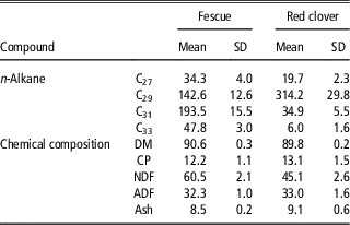
In order to minimize wastage, and to more accurately weigh the amount of forage consumed, pure fawn fescue (Festuca arundinacea) and red clover (Trifolium pratense) hay was shredded, and pressed to form 3.18 ×3.18 cm cubes, with steam as a moistening agent to facilitate the process (McHay Company, Elgin, OK, USA). Cubes were processed, bagged and stored. Sufficient feed was processed as a single batch for use at both physiological stages. Both forages were analyzed for CP, NDF, ADF and ash contents (Table 1).
Mean n-alkane concentration (mg/kg dry matter (DM)) and chemical composition of fescue and red clover fed to beef cattle heifers

Animals had ad libitum access to feed from either forage. An insert designed to hold two separate buckets was placed in each feeding bunk, with each bucket filled with a single cube-type. Each morning (0800 h) refusals from the previous day were weighed and, if dusty, discarded. The buckets were then re-filled and their weight recorded. The buckets were checked in the afternoon (1500 h) and, if necessary, additional feed weighed and added. Observed diet composition for each heifer was then determined by comparing the amount of each forage consumed in a day with the total feed consumed. Further details of the experimental layout and feeding strategy are provided in Vargas Jurado et al. (Reference Vargas Jurado, Tanner, Blevins, Rich, Mayes, Fiske, Swecker and Lewis2015).
Fecal collection
During the final 5 days of each study, fecal samples were collected twice a day, starting at 0800 and 1500 h, for all animals either by rectal grab or from the ground if the animal was identified. When possible, 200 g of fecal matter was obtained from each animal. Samples were placed in individual aluminum containers, and oven dried at 65°C for 6 to 8 days, or until 1 g or less of difference in weight was noted. The dried samples were then ground on a Wiley Mill (Thomas Scientific, Swedesboro, NJ, USA) through a 1-mm screen and stored until analysis. Average dietary choices estimated and observed over these 5 days of fecal collection were compared for individual heifers.
Laboratory analyses
Extractions were performed on each forage and fecal sample in duplicate as outlined in Dove and Mayes (Reference Dove and Mayes2006). Briefly, 0.2 g of a forage, or 0.1 g of a fecal, sample was weighed into glass tubes and approximately 0.1 g of a solution containing 0.3 mg/g of n-docosane (C22) and n-tetratriacontane (C34). These samples were heated with 1 M ethanolic KOH for 16 h at 90°C, using a dry-block heater. Heptane and distilled water were added to each warmed tube, and the non-aqueous layer was collected after shaking vigorously. Hydrocarbons were collected by solid-phase extraction and heptane elution through a silica gel column.
Quantification of ALK was performed using an Agilent 6890N gas chromatograph (GC; Agilent Technologies Inc., Santa Clara, CA, USA). The ALK fractions were injected (0.5 ml) into a splitless liner via either a 7650A Series or a 7683B series auto-sampler onto a bonded-phase, non-polar column (Agilent Technologies Inc., Santa Clara, CA, USA: Agilent J&W DB-1 column, 30 m, 0.53 mm internal diameter and 0.5 μm film thickness). Helium served as the carrier gas at a constant flow of 4 ml/min. Temperature was 280°C for the injector and 340°C for the detector. The column was held at 170°C for 4 min, then programmed at 30°C/min to 215°C with an isothermal hold of 1 min, and a second temperature ramp of 6°C/min to 300°C with a final 20 min hold time. Samples of ALK standard solution mixtures (C21 to C36; Sigma-Aldrich, St. Louis, MO, USA) were included in the GC analyses to identify peaks and standard response factors. Chromatographic data were analyzed using Agilent ChemStation software (Rev. B.04.02 SP1). Peak areas were determined with auto-integration and manual review of chromatograms. The ALK concentrations were calculated relative to known amounts of the internal standards (C22, C34), according to Dove and Mayes (Reference Dove and Mayes2006).
Statistical analyses
Correction factors
As plant-wax markers are not always fully recovered in feces, their concentration needs to be corrected to avoid biases in estimation of diet composition. Fecal recovery rates for ALK were compiled from Dove et al. (Reference Dove, Mayes and Freer1996), Brosh et al. (Reference Brosh, Henkin, Rothman, Aharoni, Orlov and Arieli2003), Van den Pol-Van Dasselaar (Reference van den Pol-Van Dasselaar, Valk and de Visser2006), Elwert et al. (Reference Elwert, Dove and Rodehutscord2006) and Olivan et al. (Reference Olivan, Ferreira, Celaya and Osoro2007); and for long-chain alcohols (LCOH) from Lin et al. (Reference Lin, Zhu, Jiang, Luo, Wang, Zhang and Hong2012), Ferreira et al. (Reference Ferreira, Celaya, Santos, Guedes, Rodrigues, Mayes and Osoro2012) and López López et al. (Reference López López, Celaya, Santos, Rodrigues, Osoro and Ferreira2015). Reported ALK fecal recovery values ranged from 0.49 for C25 to 1.00 for C35 and, similarly, LCOH fecal recovery ranged from 0.50 for C20OH to 1.00 for C36OH. The CV for ALK were 0.17, 0.13, 0.10, 0.09, 0.08 and 0.05 for C25, C27, C29, C31, C33 and C35, respectively, while the CV for LCOH were 0.21, 0.27, 0.26, 0.20, 0.09 and 0.11 for C22OH, C24OH, C26OH, C28OH, C30OH and C32OH, respectively.
Recovery fractions are naturally bounded between zero and one, approaching one as the number of carbon atoms in the chain increases. Across markers, the distribution of recovery rates reported in the literature was markedly skewed, invalidating assumptions of normality. Therefore, to accommodate this intrinsic characteristics of recovery rates, a quadratic term has usually been included as a covariate when estimating the adjustment factors. The quadratic regression model can be specified as
 $$y_{i} \,\sim\,N\left( {\mu _{i} , \sigma ^{2} } \right);\mu _{i} {\equals}\beta _{0} {\plus}\beta _{1} x_{i} {\plus}\beta _{2} x_{i}^{2} $$
where y i represented the recovery fraction for the ith observation (i = 1, … , 61 for ALK, 1, … , 24 for LCOH), x i and  $x_{i}^{2} $ were the number of carbon atoms and their corresponding squared values for an ALK (or LCOH), respectively and β k (k = 0, 1, 2) were the intercept, linear and squared regression coefficient, respectively. Finally, σ 2 was the residual variance. The model above was fitted to the literature values of recovery rates using the ‘lm’ function in R (R Core Team, 2017).
A more mathematically pertinent approach to model recovery rates would be to fit a beta regression model since the domain of a beta random variable is (0, 1), thus accommodating its bounds directly. The Beta regression model was specified as
 $$\eqalignno{ y_{i} \,\sim\,\rm Beta \left( {\mu _{i} ,\phi } \right);\eta _{i} & {\equals}\log \left( {{{\mu _{i} } \over {1{\minus}\mu _{i} }}} \right){\equals}\beta _{0} {\plus}\beta _{1} x_{i} ,\cr & \mu _{i} {\equals} {{\exp \left( {\beta _{0} {\plus}\beta _{1} x_{i} } \right)} \over {1{\plus}\exp \left( {\beta _{0} {\plus}\beta _{1} x_{i} } \right)}}$$
where μ i and ϕ were the mean and scale parameter, respectively, and  $\eta _{i} $ was the linear predictor. The regression parameters (intercept and slope) were now on a logit scale, and in this scenario, it was not necessary to include a quadratic term. Model (2) was fitted using the ‘betareg’ function from the ‘betareg’ package (Cribari-Neto and Zeileis, Reference Cribari-Neto and Zeileis2010) in R.
To account for the variation resulting from using data collected from different literature sources, diets and livestock species both regression models were fitted using a leave-one-out cross-validation scheme, and the final estimates of recovery were the ones that provided the least cross-validation error.
Combining fecal collections
Separately, within the a.m. and p.m. fecal collections, a subsample of equal dry weight of the daily collections were combined into pools. The ALK concentrations of these pools were obtained. This allowed four approaches for estimated dietary choices: (i) from ALK concentrations of the a.m. pool; (ii) from the ALK concentrations of the p.m. pool; (iii) from the simple average of the dietary choices estimated for the a.m. and p.m. pools; and, lastly, (iv) from the average of the ALK concentrations of the a.m. and p.m. pools.
Fecal n-alkane concentration
Multivariate ANOVA was used to test whether there were differences in ALK fecal concentrations across physiological stages and approaches to combine fecal collections. A model including both effects was fitted using the ‘lm’ function in R. In addition, due to the multivariate nature of ALK concentration data, relationships between markers were likely to be present. To test whether these covariances remain homogeneous across physiological stages and approaches to combine fecal collections a Box’s M-test was performed. A multivariate CV (MCV) was also calculated for ALK fecal concentrations as described by Voinov and Nikulin (Reference Voinov and Nikulin1996), namely
 $$MCV{\equals}\left( {{\hat{\mu }}^{'} {\hat{\Sigma }}^{{{\minus}1}} {\hat{\mu }}} \right)^{{{\minus}1\,/\,2}} $$
where  ${\hat{\mu }}{\equals}\left[ {\hat{\mu }_{{C_{{27}} }} \;\hat{\mu }_{{C_{{29}} }} \;\hat{\mu }_{{C_{{31}} }} \;\hat{\mu }_{{C_{{33}} }} } \right]$ is the estimated vector of mean ALK fecal concentrations, and
 ${\hat{\Sigma }}$ is the estimated ALK fecal (co)variance matrix.
Diurnal variation in n-alkane fecal concentration
Differences between daily a.m. and p.m. ALK concentrations were tested using a linear model
 $$\eqalignno{ y_{{ijklm}} {\equals}&\mu {\plus}S_{i} {\plus}C_{j} {\plus}D_{k} {\plus}(SC)_{{ij}} {\plus}(SD)_{{ik}} {\plus} \cr & (CD)_{{jk}} {\plus}(SCD)_{{ijk}} {\plus}(HD)_{kl}{\plus}{\varepsilon}_{m} $$
where y ijklm was the fecal concentration for the a given ALK, S i the effect of the ith physiological stage (i = 1, 2), C j the effect of the jth fecal collection strategy (j = 1, 2), D k the effect of the kth day (k = 1, …, 5), (SC)ij, (SD)ik, (CD)jk and (SCD)ijk were their interaction effects,  $\left( {HD} \right)_{{kl}} $ the effect of heifer l measured at day k and finally ε m the residual. Both
 $\left( {HD} \right)_{{kl}} $ and ε m were fitted as random effects. In addition, differences between ALK concentrations in the pooled a.m. and pooled p.m. were tested using a linear model similar to (4) but without the day effect or its interactions.
Estimation of diet composition
The amount of fescue and red clover in the diet of each animal was estimated from four ALK found in the forages and feces: C27, C29, C31 and C33. Estimates were obtained using two statistical methods: (i) by fitting a BLHU model (Vargas Jurado et al., Reference Vargas Jurado, Eskridge, Kachman and Lewis2018), and (ii) by using NNLS (Dove and Moore, Reference Dove and Moore1995). The BHLU model was implemented in R using the ‘Rcpp’ package (Eddelbuettel and Francois, Reference Eddelbuettel and Francois2011) and described by Vargas Jurado et al. (Reference Vargas Jurado, Eskridge, Kachman and Lewis2018). In addition, NNLS was implemented through the ‘nnls’ package in R. This technique best matches the ALK profile in the forages to that of a fecal sample (Dove and Moore, Reference Dove and Moore1995; Newman et al., Reference Newman, Thompson, Penning and Mayes1995).
Accuracy of estimated diet composition
Given that the ‘true’ forage proportions for each animal were measured in both experiments, the accuracy of the estimates was assessed through the use of mean squared error (MSE), relative mean squared error (ReMSE) and reconstruction error (RE), defined as
 $$\eqalignno{{\rm MSE}{\equals} & {1 \over n}\mathop {\sum\parallel}\limits_{i{\equals}1}^n {\hat{\theta }}_{i} {\minus}{\bf \theta }_{i} \parallel_{{}}^{2}; {\rm ReMSE}{\equals}{1 \over n}\mathop \sum\limits_{i{\equals}1}^n \parallel{{{\hat{\theta }}_{i} {\minus}{\bf \theta }_{i}^{{}} } \over {{\bf \theta }_{i} }}\parallel_{{}}^{2} , \cr & {\rm RE}{\equals}\sqrt {{1 \over n}\mathop \sum\limits_{i{\equals}1}^n \parallel{\bf y}_{i} {\minus}{\bf M} \hat {\theta _{i}}} \parallel_{{}}^{2} } $$
where  ${\hat{\theta }}_{i} $ was the estimated proportion of clover for the ith heifer,
 ${\bf \theta }_{i} $ the vector of true (observed) diet proportions and ||·||2 the squared Euclidean norm, and yi and
M were as before the vector of fecal ALK concentrations for the ith heifer, and the matrix of ALK concentrations for fescue and red clover, respectively. For all three criteria, lower values represent better performance.
The observed and estimated proportions of red clover in the diet were compared by regressing the observed on estimated red clover. The hypotheses tested were that the slope was not differed from unity, and that the intercept was not differed from zero. Tests were performed for each physiological stage, fecal collection scheme and statistical method separately.
To formally test whether differences between observed and estimated proportions of red clover in the diet existed, the natural logarithm of that difference (logDIFF) was tested using ANOVA in R. The back-transformation of logDIFF should be close to one if the dietary observed and estimated red clover proportions are similar, less than one if the observed proportion is overestimated, and greater than one if the observed proportion is underestimated. The following linear model was assumed
 $$\eqalignno{ \log DIFF_{{ijkl}} {\equals}& \mu {\plus}S_{i} {\plus}C_{j} {\plus}M_{k} {\plus}\left( {SC} \right)_{{ij}} {\plus}\left( {SM} \right)_{{ik}} {\plus} \cr & \left( {CM} \right)_{{jk}} {\plus}\left( {SCM} \right)_{{ijk}} {\plus}{\epsilon}_{{ijkl}} $$
where μ was the overall  $\log DIFF_{{ijkl}} $ value, S i the effect of the ith physiological stage (i = 1, 2), C j the effect of the jth fecal collection scheme (j = 1, 2, 3), M k the effect of the kth statistical method for estimating diet proportions (k = 1, 2). The (SC)ij, (SM)ik, (CM)jk and (SCM)ijk were the two- and three-way interactions, respectively, and ε ijkl the residual. All the effects above (except for the residual) and their interactions were included as fixed effects. Estimates and confidence intervals were presented on the back-transformed scale.
Results
Correction factors
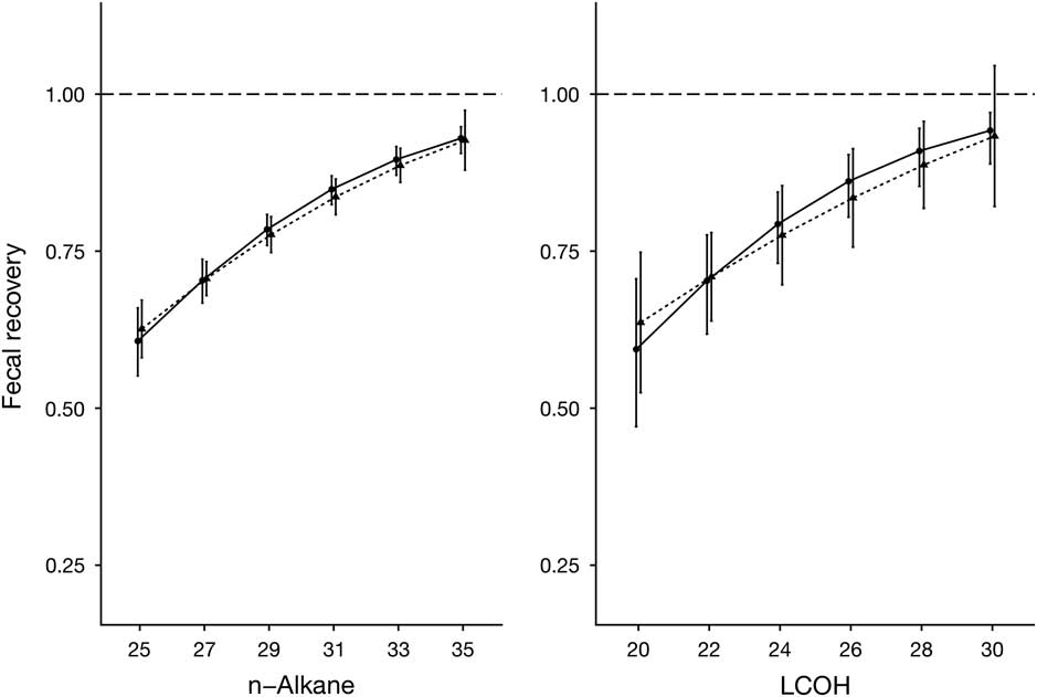
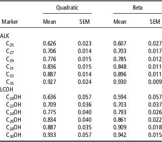
In general, there was less variation in the recoveries reported in literature for ALK than those for LCOH. Recoveries for both type of markers were similar for quadratic and Beta regression. However, the accuracy of the estimates was higher for ALK (Table 2), especially for markers with higher number of carbon atoms, where recoveries tended to be close to one. Standard errors also were smaller for ALK than for LCOH. In the latter case, fitting the quadratic regression resulted in 95% confidence intervals higher than one for C30OH. Such was not the case with the Beta regression (Figure 1). Based on predictive performance on both ALK and LCOH data, the estimates derived from Beta regression were used for estimating diet proportions.
Estimated recovery fractions for n-alkane (ALK) and long-chain alcohol (LCOH) relative to number of carbon atoms in the compound compiled from literature and used to correct fecal ALK concentrations in beef cattle heifers. Solid line is from the fit of a Beta regression and dot-dashed line is from the fit of a quadratic regression.

Estimated fecal recoveries (compiled from literature) for n-alkanes (ALK) and long-chain alcohols (LCOH) derived from the fits of quadratic and Beta regressions used to correct ALK fecal concentrations in beef cattle

n-Alkane fecal concentration
Fecal ALK concentrations measured at the post-weaning and yearling studies differed (P < 0.001). Fecal C27, C31 and C33 concentrations were 1.05, 1.06 and 1.01 times larger, respectively, at the yearling stage. On the other hand, fecal C29 concentration was 1.22 times larger at the yearling compared to post-weaning stage. In the same manner, ALK concentrations measured on pooled a.m. collections were different from those measured on pooled p.m. collections (P < 0.001). Fecal C27, C31 and C33 concentrations were 1.08, 1.12 and 1.06 times larger when measured on pooled p.m. collections, whereas C29 was 1.16 times larger.
Once corrected for incomplete fecal recovery, the estimated ALK covariance matrix at post-weaning ( ${\hat{\Sigma }}_{p} $) did not differ from the one at the yearling study (
 ${\hat{\Sigma }}_{y} $; P = 0.22). Still,
 ${\rm trace}({\hat{\Sigma }}_{y} )$ was about 1.76 times
 ${\rm trace}({\hat{\Sigma }}_{p} )$, indicating larger overall variation at the yearling stage. Similarly, covariance matrices did not differ between approaches for combining fecal collections (P = 0.14). Estimated covariance matrices from pooled a.m. ALK fecal concentrations (
 ${\hat{\Sigma }}_{{am}} $) did not differ from the one estimated from p.m. pooled ALK concentrations (
 ${\hat{\Sigma }}_{{pm}} $), or from mean ALK (
 ${\hat{\Sigma }}_{{mean}} $). However,
 ${\rm trace}({\hat{\Sigma }}_{{pm}} )$ was about 1.98 times
 ${\rm trace}({\hat{\Sigma }}_{{am}} )$, and about 2.21 times
 ${\rm trace}({\hat{\Sigma }}_{{mean}} )$ clearly showing more overall variability for ALK fecal concentrations from pooled p.m. collections.
Multivariate CV were 0.19 and 0.25 for the post-weaning and yearling studies respectively, also indicating larger variability in ALK fecal concentrations. Furthermore, MCV were 0.19, 0.24 and 0.16 for a.m., p.m., and average a.m. and p.m. ALK concentration, respectively, showing that averaging fecal ALK concentrations reduced variation.
When comparing the ALK concentrations of the daily a.m. and p.m. fecal collections (model (4)), no differences were observed regardless of physiological stage (P > 0.12). Although p.m. measurements tended to be more variable, no clear diurnal variation in ALK fecal concentrations were apparent.
Estimated diet choice
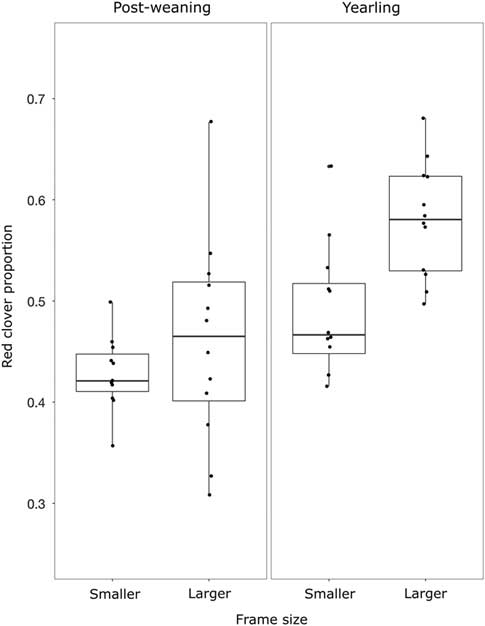
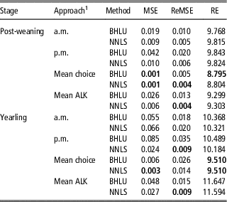
Box-plots of observed dietary choices across physiological stages (post-weaning, yearlings) and frame sizes are presented in Figure 2. In general, diet choices were estimated more reliably when based on dietary choices obtained from the a.m. and p.m. fecal samples and then averaged (Table 3). Errors were low in general for both the BHLU and NNLS methods. However, the relative performance of these statistical methods was not consistent, as measured by MSE, ReMSE and RE.
Observed diet composition of beef cattle heifers at two physiological stages (post-weaning, yearling) and two frame sizes (smaller, larger).

Efficiency for Bayesian hierarchical linear unmixing model (BHLU) and non-negative least squares (NNLS) for dietary choices of beef cattle heifers estimated in four ways

MSE = mean squared error; ReMSE = Relative mean squared error; RE = reconstruction error.
Best method for each criterion shown in bold.
1 Dietary choice based on the n-alkane (ALK) concentrations of the a.m. or p.m. pools, the average ALK concentrations of those pools (mean ALK) and the simple mean of the dietary choices from the a.m. and p.m. pools (mean choice).
At post-weaning, lower MSE and ReMSE were achieved when ALK concentrations were averaged across the a.m. and p.m. fecal samples and estimated based on NNLS; however, the lowest RE was achieved when using BHLU. At the yearling study, however, the lowest value for all criteria was obtained by NNLS using ALK concentrations averaged across the p.m. fecal samples. In addition, NNLS and BHLU performance was reduced at the yearling as compared to post-weaning study since MSE, ReMSE and RE values were higher (Table 3).
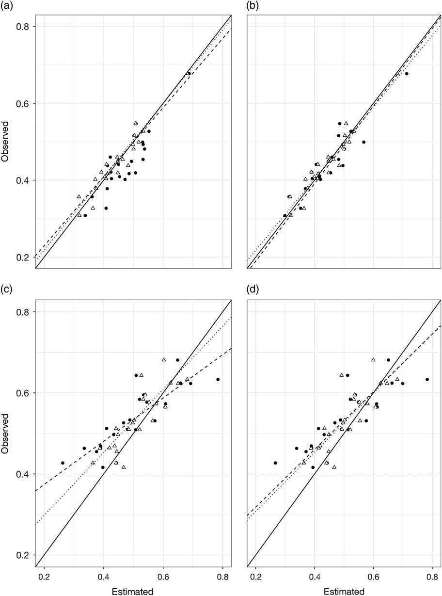
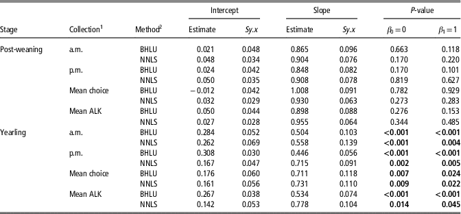
At post-weaning, estimates of the intercept always included zero, and the estimates of the slope always included one, regardless of the approach used to combine fecal ALK concentrations or statistical method (P > 0.101; Table 4, Figure 3). However, at the yearling stage, estimates of the intercept and slope differed from zero and one, respectively, regardless of the ALK fecal combination strategy or statistical method (P < 0.045).
Estimated red clover proportion regressed on observed red clover proportion in the diet of beef cattle heifers. Top panels show fit of the average n-alkane concentration of the a.m. and p.m. pools, and bottom panels show fit of the simple mean of the dietary choices from the a.m. and p.m. pools. Solid line at 45° angle represents a perfect fit, dashed line and black circles show Bayesian hierarchical linear unmixing fit, and dotted lines with white triangles show non-negative least squares fit. Plots (a) and (b) correspond to post-weaning age, and plots (c) and (d) correspond to yearling age.

Test for estimates of intercept and slopes based on regressing observed on estimated red clover proportion in the diet of beef cattle heifers

1 Dietary choice based on the n-alkane (ALK) concentrations of the a.m. or p.m. pools, the average ALK concentrations of those pools (mean ALK), and the simple mean of the dietary choices from the a.m. and p.m. pools (mean choice).
2 Statistical methods were Bayesian hierarchical linear unmixing model (BHLU) and non-negative least squares (NNLS).
P-values less than 0.05 are highlighted in bold text.
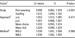
The ratios between dietary proportions of estimated and observed red clover proportion were close to one in general with a mean of 1.02 but with considerable variability (SD = 1.25). In the post-weaning study, the ratio of estimated to observed red clover proportion in the diet ranged from 0.51 to 2.17. On the other hand, in the yearling study that ratio of dietary proportion of estimated to observed red clover ranged from 0.67 to 1.85. While there was no effect of the approach used to combine ALK concentrations of fecal samples (P = 0.42) or statistical method (P = 0.96) on this ratio, there was a substantial effect of physiological stage (P < 0.001). In addition, none of the two- or three-way interactions between these factors were found to be significant. Least-squares means for these ratios are presented in Table 5.
For the difference between observed and estimated red clover proportion in the diet of beef cattle heifers, least-squares means (LS means), 0.95 confidence interval (CI) and significance (P-value) for physiological stage, fecal collection strategy and statistical method

1 Main effect LS means for physiological stage, fecal combination strategy and statistical method.
2 Dietary choice based on the n-alkane (ALK) concentrations of the a.m. or p.m. pools, the average ALK concentrations of those pools (mean ALK), and the simple mean of the dietary choices from the a.m. and p.m. pools (mean choice).
3 Statistical methods were Bayesian hierarchical linear unmixing model (BHLU) and non-negative least squares (NNLS).
Discussion
n-Alkane contents of forages
The concentration of the major ALK in the forages used appears to be different enough to allow for the estimation of diet choice. These ALK values are similar to those reported by Dove and Mayes (Reference Dove and Mayes2006) for fescue and Elwert et al. (Reference Elwert, Dove and Rodehutscord2008) for red clover. However, Vargas Jurado et al. (Reference Vargas Jurado, Tanner, Blevins, McNair, Mayes and Lewis2014) found that the LCOH concentrations of the tall fescue and red clover hays used in the current study were not sufficiently different to contribute to more accurate estimates of dietary choice.
Correction factors
Fecal recoveries were more accurately estimated (lower standard error) for ALK than those of LCOH, which was somewhat expected given the larger number of literature sources for the former. In addition, LCOH recoveries appear in general to be more variable (Lin et al., 2012; Ferreira et al., Reference Ferreira, Celaya, Santos, Guedes, Rodrigues, Mayes and Osoro2012). Assuming a Beta distribution for fecal recoveries resulted in more accurate estimates especially for those ALK or LCOH with longer carbon chains (Table 2, Figure 1). This was because it automatically accounts for the heteroscedastic nature of proportions (Ferrari and Cribari-Neto, Reference Ferrari and Cribari-Neto2004). Although quadratic regression produced a good fit for ALK data, standard errors were still large even for ALK with longer carbon-chains (recovery fractions closer to one).
Measures of fit such as R 2 (or similar statistics) could not be used since the Beta regression model fits a link function, while the quadratic regression does not. Ferreira et al. (Reference Ferreira, Celaya, Santos, Guedes, Rodrigues, Mayes and Osoro2009) reported that the fecal recoveries for individual ALK may not only be specific to an animal species (i.e. sheep, goats, cattle), but also depend on the diet. Similarly, Elwert et al. (Reference Elwert, Dove and Rodehutscord2008) reported varying ALK recoveries for sheep fed different diets, justifying the use of leave-one-out cross-validation to account for the variation in reported recovery rates in this study. Other researchers have mentioned the usefulness of cross-validation in nutrition studies (Decruyenaere et al., Reference Decruyenaere, Planchon, Dardenne and Stilmant2015; Núñez-Sanchez et al., Reference Núñez-Sánchez, Carrion, Peña Blanco, García, Garzón Sigler and Martínez-Marín2016).
Since derived from a number of literature sources, these fecal recovery rates may provide a useful approximation when study-specific recoveries were unavailable. They would be applied by dividing the observed ALK and LCOH fecal concentrations by their respective recovery rate in Table 2.
n-Alkane fecal concentration
Since feed sources (hay) remained constant at both physiological stages, variation in ALK fecal concentration was likely due to changes in dietary choices. However, an overall increase in variation was not anticipated. Due to the simplicity of NNLS, extraneous sources of variation may affect estimates of diet choice when using plant-wax markers. This increased variation should not be an issue with BHLU, since it allows for an unstructured error covariance matrix. However, with a limited sample size, as was the case in this study, estimates of (co)variances were likely not accurate, thus introducing uncertainty into estimation of dietary choices.
Estimated diet choice
Variation between and within individual heifers when yearlings in their ALK fecal concentrations reduced accuracy of estimation of their dietary choices. On the other hand, at post-weaning dietary choices were estimated reliably. The latter results are in accordance with Brosh et al. (Reference Brosh, Henkin, Rothman, Aharoni, Orlov and Arieli2003) who reported accurate estimates of diet composition once correcting for incomplete fecal recovery.
In both physiological stages, diet choices were more accurately estimated by first obtaining their values from the individual fecal samples (separately for the a.m. and p.m. pools) and then averaging those estimates. However, analyzing the ALK concentrations of a single fecal sample on an animal would be much more economical. Although estimates of dietary choices tended to be more reliable when combining separate choice estimates, the differences were relatively small compared to those obtained from single pooled fecal samples. Albeit slightly less accurate, pooling (combining) daily (or twice daily) fecal samples into a single aggregate sample aided in alleviating diurnal variation and was substantially more cost effective.
Heifers were managed so that feeding was mostly undisturbed. Still, fecal samples were collected twice daily, which could have affected individual feeding habits thereby introducing diurnal variation in ALK excretions. However, no clear pattern was observed in this study for either physiological stage. Oliveira et al. (Reference Oliveira, Medeiros, Tedeschi, Silva and Lanna2015) reported variation in the fecal ALK profile when working with dairy cattle grazing on tropical pasture and attributed those changes to differences in rumen fill due to more intense grazing in the afternoon. Moreover, Bani et al. (Reference López López, Celaya, Santos, Rodrigues, Osoro and Ferreira2014) reported a significant decrease in C31 fecal concentration between morning and afternoon sampling. A similar trend, albeit not significant, was also reported for C33 fecal concentration (Bani et al., Reference López López, Celaya, Santos, Rodrigues, Osoro and Ferreira2014).
The three measures of accuracy used did not consistently identify which of the two statistical methods was more reliable at estimating diet composition at post-weaning; however, NNLS was consistently more accurate at the yearling stage. As seen in Figure 3, the fitted line from regressing observed on estimated red clover proportion in the diet using BHLU and NNLS is very close to the optimal line (at a 45° angle) particularly at post-weaning, with some variation around intercepts and slopes. At yearling age, the fit of regression using NNLS was better than with BHLU.
Elwert et al. (Reference Elwert, Dove and Rodehutscord2008) reported much less variation among estimates of the intercepts, which ranged from −0.005 to 0.014, and slopes, which ranged from 0.963 to 1.008, for the regression of observed on estimated dietary choices than obtained in the current study. However, other sources of variation, such as physiological stage and fecal collection strategy, clearly contributed to the greater variability among estimates reported in Table 4.
Despite the variation encountered, differences between observed diet choices and those estimated by BHLU or NNLS were minimal, with similar performance at both physiological stages. However, the interaction between physiological stages and statistical method makes conclusions about overall performance less evident. Elwert et al. (Reference Elwert, Dove and Rodehutscord2008) reported differences between observed and estimated barley proportion in different diets fed to sheep, which ranged from −0.026 to 0.005 depending on the type of diet. Similarly, mean differences between estimated and observed red clover proportions found in the present study ranged from −0.032 to 0.050 and −0.008 to 0.032 for BHLU and NNLS, respectively.
Delineating forages species using plant-waxes largely depends on the uniqueness of their ALK and LCOH profiles. Thus generalization of the accuracy of the methodology to more diverse swards is therefore difficult. However, Bezabih et al. (Reference Bezabih, Pellikaan and Hendriks2011), Lewis et al. (Reference Lewis, Vargas Jurado, Hamilton and Volesky2016) and Vargas Jurado et al. (Reference Vargas Jurado, Eskridge, Kachman and Lewis2018) did report a consistent increase in estimation error (MSE) when increasing the number of forage species in mixtures from 5 to 15.
Conclusion
The ALK technique provided a reliable tool for the estimation of diet choice in heifers at post-weaning when offered a simple diet. Such was less the case at yearling age, where greater variation in fecal ALK concentrations reduced the accuracy of estimation. Still, by combining (pooling) twice daily fecal samples into an aggregate sample, and with the application of correction factors to account for incomplete fecal recovery of ALK, this technique offers opportunity to determine diet choice in experimental (controlled) settings. Averaging individual estimates of diet composition resulted in slightly higher accuracy than that obtained from pooled fecal samples. Nevertheless, given laboratory costs associated with the increased number of samples to be analyzed, the gain in accuracy from averaging individual estimates of diet composition is not necessarily justified. Using pooled fecal samples over a 5-day period provides a pragmatic application of this methodology to estimate the composition of a simple diet.
Acknowledgements
This project was supported by the US Department of Agriculture (USDA), Agricultural Research Service (ARS), Award Number 1932–21630–003–06. The authors appreciate the scientific advice and contribution of Dr Robert Mayes (The James Hutton Institute, Craigiebuckler, Aberdeen, Scotland, UK), and the technical assistance of Jessica Rich (Virginia Tech, Blacksburg, Virginia, USA). The authors are also thankful to Donald Wirth (Saddle Butte Ag Inc., Shedd, OR, USA) for supplying the forages (hays) and to Phillip and Edgar McCracken (McHay Company, Elgin, OK, USA) for feed processing (cubing). This project was completed in partial fulfillment of the first author’s thesis.
Declaration of interest
The authors declare no conflicts of interest.
Ethics statement
All the techniques and procedures used were approved and performed in compliance with the Institutional Animal Care and Use Committee at Virginia Tech.
Software and data repository resources
None of the data were deposited in an official repository. An R package implementation of the BLHU model can be found at https://github.com/napovargas/BHLU.