1. Introduction
For an oblique shock impinging on the bow shock in front of a blunt body, Edney (Reference Edney1968) discovered six types of shock interferences as shown in figure 1. Shock interference has a significant influence on the design of supersonic vehicles (Jenkins Reference Jenkins2007). Extensive research has been conducted on aspects as follows: aerodynamic and aerothermal loading (Hains & Keyes Reference Hains and Keyes1972; Keyes & Morris Reference Keyes and Morris1972; Keyes & Hains Reference Keyes and Hains1973; Holden et al. Reference Holden, Moselle, Wieting and Glass1988; Wieting & Holden Reference Wieting and Holden1989; Vemaganti Reference Vemaganti1994; Zhong Reference Zhong1994; Boldyrev et al. Reference Boldyrev, Borovoy, Chinilov, Gusev, Krutiy, Struminskaya, Yakovleva, Délery and Chanetz2001; Grasso et al. Reference Grasso, Purpura, Chanetz and Délery2003; Wang et al. Reference Wang, Li, Zhang and Yang2020; Wang et al. Reference Wang, Han, Liu and Jiang2023a, Reference Wang, Liu and Li2025; Zhang et al. Reference Zhang, Zhang, Rao, Shi, Zhu and You2025); unsteady oscillation (Gaitonde & Shang Reference Gaitonde and Shang1995; Lind & Lewis Reference Lind and Lewis1996; Furumoto & Zhong Reference Furumoto and Zhong1997; Yamamoto, Kano & Daiguji Reference Yamamoto, Kano and Daiguji1998; Ben-Dor et al. Reference Ben-Dor, Vasilev, Elperin and Zenovich2003; Hu et al. Reference Hu, Myong, Wang, Cho and Jiang2008; Xiao et al. Reference Xiao, Li, Zhu and Yang2017; Khatta & Gopalan Reference Khatta and Gopalan2018; Kianvashrad & Knight Reference Kianvashrad and Knight2023); the effects of thermal non – equilibrium, chemical non – equilibrium and rarefaction effects (Furumoto, Zhong & Skiba Reference Furumoto, Zhong and Skiba1996; Zhong & Lee Reference Zhong and Lee1996; Yamamoto, Takasu & Nagatomo Reference Yamamoto, Takasu and Nagatomo1999; Sanderson, Hornung & Sturtevant Reference Sanderson, Hornung and Sturtevant2004; Tchuen, Burtschell & Zeitoun Reference Tchuen, Burtschell and Zeitoun2011; White & Kontis Reference White and Kontis2017; Garbacz et al. Reference Garbacz, Morgado and Fossati2022, Reference Garbacz, Morgado and Fossati2023; Wang et al. Reference Wang, Guo, Hong and Li2023b; Li et al. Reference Li, Sun, Dai, Chen, Zhang and Man2024); and flow field prediction (Bramlette Reference Bramlette1974; Frame & Lewis Reference Frame and Lewis1997; Peng et al. Reference Peng, Luo, Han, Hu, Han and Jiang2020).
Schematics of six types of shock interference.

Six types of shock interference are summarised as follows (Edney Reference Edney1968): Type I and II shock interferences arise when the oblique shock interferes with the weak shock segment of a bow shock, where the weak shock segment belongs to the different family from the oblique shock; Type III and Type IV shock interferences arise when the oblique shock interferes with the strong shock segment of a bow shock; Type V and Type VI shock interferences arise when the oblique shock interferes with the weak shock segment of a bow shock, where the weak shock segment belongs to the same family as the oblique shock.
After the work by Edney (Reference Edney1968), many related experiments and computational works have confirmed the existence of six types of shock interference (Grasso et al. Reference Grasso, Purpura, Chanetz and Délery2003; Peng et al. Reference Peng, Luo, Han, Hu, Han and Jiang2020; Peng et al. Reference Peng, Li, Yang, Lin, Han and Hu2023; Yang et al. Reference Yang, Cui, Tian, Li, Xiao and Chang2025). Grasso et al. (Reference Grasso, Purpura, Chanetz and Délery2003) summarised the transition processes between different interferences as follows: the transition between Type I and Type II shock interference corresponds to that between regular reflection and Mach reflection (Grasso et al. Reference Grasso, Purpura, Chanetz and Délery2003). Two transition criteria (detached condition and von Neumann condition) were established by von Neumann (Reference von Neumann1943, Reference von Neumann1945). A number of studies demonstrated that hysteresis processes exist between regular reflection and Mach reflection (Ivanov et al. Reference Ivanov, Zeitoun, Vuillon, Gimelshein and Markelov1996; Vuillon, Zeitoun & Ben-Dor Reference Vuillon, Zeitoun and Ben-Dor1996; Li, Chpoun & Ben-Dor Reference Li, Chpoun and Ben-Dor1999; Ivanov et al. Reference Ivanov, Ben-Dor, Elperin, Kudryavtsev and Khotyanovsky2001, Reference Ivanov, Ben-Dor, Elperin, Kudryavtsev and Khotyanovsky2002); the transition between Type II and Type III shock interference occurs when the oblique shock interacts with the bow shock at the lower sonic point
 $A$
(as shown in figure 1) where the flow behind the bow shock is sonic; the transition between Type III and Type IV shock interference occurs when the flow deflection angle at point
 $C$
(as shown in figure 1) is equal to the local detachment angle; the transition between Type IV and Type V shock interference occurs when the oblique shock interacts with the bow shock at the upper sonic point
 $B$
(as shown in figure 1) where the flow behind the bow shock is sonic.
Many new types of shock interference have been reported in the literature. According to the wave configuration, Peng et al. (Reference Peng, Li, Yang, Lin, Han and Hu2023) revealed a new type between Type III and Type IV interference, named Type IIIa. According to the shape of the jet, Type IV shock interference has two other sub-types: Type IVa interference occurs when the jet is deflected upwards and only grazes the blunt body surface (Boldyrev et al. Reference Boldyrev, Borovoy, Chinilov, Gusev, Krutiy, Struminskaya, Yakovleva, Délery and Chanetz2001); Type VII shock interference occurs when the jet may bend upwards without stagnating on the body (Yamamoto et al. Reference Yamamoto, Takasu and Nagatomo1999). According to the Mach number behind the reflected shock at triple point
 $T_2$
, Type IV shock interference can be divided into three types, distinguished by subsonic, transonic or supersonic jets (Guan, Bai & Wu Reference Guan, Bai and Wu2020; Bai & Wu Reference Bai and Wu2022). Bai & Wu (Reference Bai and Wu2022) proposed criteria for these three different situations and discovered that the transonic jet has a two-branch structure: the lower branch is subsonic, the upper branch is supersonic.
In addition, triple points exist not only in Type IV shock interference but also widely in other types of shock interference, the black points in figure 1 denote these triple points. Generally, the flow near a triple point is a Mach reflection. However, the change of the strength of the incident shock at a triple point may cause other types of reflection to occur: von Neumann reflection, Vasilev reflection or Guderley reflection (Guderley Reference Guderley1947; Colella & Henderson Reference Colella and Henderson1990; Vasilev & Kraiko Reference Vasilev and Kraiko1999; Skews & Ashworth Reference Skews and Ashworth2005; Vasilev, Elperin & Ben-Dor Reference Vasilev, Elperin and Ben-Dor2008). Based on the evolution of the triple point of the shock interference, more unknown types will probably be found. In addition, aerodynamic and thermal loading induced by shock interference depend on the interference patterns, thus the discovery of possible new sub-types should be important for accurate prediction of aerodynamic and thermal loading.
In general, wave configurations among six types of shock interference have significant differences. Although existing relevant studies have identified new types, they do not establish a complete chain between different interference types. Moreover, these works focus on the evolution of a specific type or the transition between two specific types, there is still a lack of systematic research.
In this paper, we mainly investigate the potential new sub-types between Type II and Type V shock interference. In § 2, we review the shock theory and introduce the numerical method used in this paper. In § 3, the transition processes between Type II and Type III, Type III and Type IV, and Type IV and Type V are studied. In § 4, a large number of numerical results are analysed for the global research on shock interference.
2. Transition criteria between different types of shock reflection and numerical method
In this section, we review transition criteria between different types of shock reflection. In addition, the numerical method used in this paper is introduced.
In this paper,
 $p$
,
 $M$
,
 $\theta$
,
 $\beta$
and
 $\gamma$
are used to denote pressure, Mach number, flow deflection angle, shock angle and specific heat ratio. We default to a
 $\gamma$
value of 1.4. The subscript
 $u$
denotes the upstream flow parameters of a shock, the subscript
 $d$
denotes the downstream flow parameters of a shock, the subscript
 $ud$
denotes flow parameters between the upstream and the downstream of a shock.
2.1. Transition criteria between different shock reflections
As the strength of incident shock changes, shock reflection can be divided into regular reflection, Mach reflection and weak shock reflection. Mach reflection consists of an incident shock
 $i$
, a reflected shock
 $r$
, a Mach stem
 $m$
and a slipline
 $s$
, and the flow deflects upwards after passing through the reflected shock, as shown in figure 2(a). Weak shock reflection can be divided into von Neumann reflection, Vasilev reflection and Guderley reflection. For von Neumann reflection, the flow field is similar to Mach reflection, but the flow deflects downwards after passing through the reflected shock, as shown in figure 2(b). For Vasilev reflection, the triple point is replaced by a four-wave point, which means an expansion wave
 $ \textit{PM} $
occurs downstream of the reflected shock, and the flow downstream of the Mach stem is subsonic, as shown in figure 2(c). For Guderley reflection, the flow field is similar to Vasilev reflection, but the flow downstream of the Mach stem is supersonic, as shown in figure 2(d).
Schematics of shock reflection. (a) Triple point for Mach reflection. (b) Triple point for von Neumann reflection. (c) Four-wave point for Vasilev reflection. (d) Four-wave point for Guderley reflection.

Flow deflection angles of a Mach reflection satisfy
 $\theta _{03}=\theta _{01}{-}\theta _{12}$
, whereas flow deflection angles of a von Neumann reflection satisfy
 $\theta _{03}=\theta _{01}+\theta _{12}$
. Thus, transition criterion
 $\theta _{01}=\theta _{\textit{MR}}^{\textit{VNR}}(M_{0})$
(
 ${\textit{MR}}$
denotes Mach reflection,
 ${\textit{VNR}}$
denotes von Neumann reflection) satisfies
 \begin{equation} \theta _{12}=0 .\end{equation}
For
 $M_0$
, transition criterion
 $\theta _{01}=\theta _{\textit{MR}}^{\textit{VNR}}(M_{0})$
can be obtained by substituting (2.1) into the three-shock theory. The three-shock theory is given in Appendix A.
Vasilev reflection occurs when the triple point transforms to a four-wave point. The transition criterion
 $\theta _{01}=\theta _{\textit{VNR}}^{\textit{VR}}(M_{0})$
(
 ${\textit{VR}}$
denotes Vasilev reflection) corresponds to where
 $M_2$
of von Neumann reflection satisfies
 \begin{equation} M_{2}=1. \end{equation}
For
 $M_0$
, transition criterion
 $\theta _{01}=\theta _{\textit{VNR}}^{\textit{VR}}(M_{0})$
can be obtained by substituting (2.2) into the three-shock theory.
Vasilev reflection satisfies
 $M_3\lt 1$
, whereas Guderley reflection satisfies
 $M_3\gt 1$
. Thus, transition criterion
 $\theta _{01}=\theta _ {\textit{VR}}^{\textit{GR}}(M_{0})$
(
 ${\textit{GR}}$
denotes Guderley reflection) satisfies
 \begin{equation} M_{3}=1. \end{equation}
For
 $M_0$
, transition criterion
 $\theta _{01}=\theta _ {\textit{VR}}^{\textit{GR}}(M_{0})$
can be obtained by substituting (2.3) into the four-wave theory. The four-wave theory is given in Appendix B.
The transition criterion between weak shock reflection and no reflection satisfies
 \begin{equation} M_{1}=1. \end{equation}
For
 $M_0$
, transition criterion
 $\theta _{01}=\theta _{max}(M_{0})$
can be obtained by substituting (2.4) into the oblique shock relations. The oblique shock relations are given in Appendix A.
These four transition criteria are displayed in figure 3, in which we also display the detachment condition
 $\theta _{D}(M_{0})$
and the von Neumann condition
 $\theta _{N}(M_{0})$
(von Neumann Reference von Neumann1943, Reference von Neumann1945). The grey area shown in figure 3 is the domain where weak shock reflection occurs. Specifically, the lower boundary of the grey area is
 $\theta _{01}=\theta _{\textit{MR}}^{\textit{VNR}}(M_{0})$
, and the upper boundary of the grey area is
 $\theta _{01}=\theta _{max}(M_{0})$
.
Transition criteria in the plane
 $M_{0}-\theta _{01}$
.

2.2. Numerical method
For the shock interference problem, Peng et al. (Reference Peng, Li, Yang, Lin, Han and Hu2023) defined a location parameter
 ${\textit{Ir}}$
to describe the location of a oblique shock:
 \begin{equation} Ir=y_{in}/R, \end{equation}
where
 $y_{in}$
is the intercept of the oblique shock on the vertical axis and
 $R$
is the cylinder radius, as shown in figure 4(a).
Computational domain and grid independence.

The compressible Euler equations of an ideal gas are solved using the second-order advection upstream splitting method. The computational domain and boundary conditions are displayed in figure 4(a). The boundary conditions are set to two inlets at the left of the computational domain, we define the parameters of these two inlets to form an oblique shock. The boundary conditions are set to two supersonic outlets at the right of the computational domain. The blunt body is set to a free-slip wall.
To evaluate the grid independence, Mach contours for three different grids with
 $M_0=2.5$
,
 $\theta _{01}=7.994^\circ$
and
 ${\textit{Ir}}=-2.7$
are compared in figure 4(b), and the densities of three grids are listed in table 1. The result of Grid 1 is coarser than those of Grid 2 and Grid 3, and the shock position of Grid 1 deviates from those of the latter two. Mach contours of Grid 2 and Grid 3 almost overlap. Hence, we use grids with a density similar to that of Grid 2 in this paper.
The details of three grids.

3. The transition processes from Type II to Type V shock interference
In this section, the transition processes from Type II to Type V shock interference are discussed. In § 3.1, we investigate the transition process between Type II and Type III shock interference. In § 3.2, we investigate the transition process between Type III and Type IV shock interference. In § 3.3, we investigate the transition process between Type IV and Type V shock interference.
3.1. The transition process between Type II and Type III shock interference
The wave configuration of Type II shock interference is displayed in figure 5(a). It has two triple points
 $T_1$
and
 $T_2$
, triple point
 $T_1$
is located on the oblique shock below the bow shock, whereas triple point
 $T_2$
is located on the bow shock. When the oblique shock moves up, the slipline behind triple point
 $T_1$
is attached to the blunt body, Type III shock interference occurs. As shown in figure 5(b), the oblique shock intersects with the bow shock, forming a triple point
 $T_1$
, the slipline
 $T_{1}C$
emanating from triple point
 $T_1$
impacts on the blunt body surface and forms another shock.
Schematics of Type II and Type III shock interferences.

It is obvious that a quite significant difference exists between Type II and Type III shock interference. Hence, there is a problem of how Type II shock interference transits to Type III.
The type of shock interference is determined by the incoming flow Mach number
 $M_0$
, the flow deflection angle of the oblique shock
 $\theta _{01}$
and the position parameter
 ${\textit{Ir}}$
of the oblique shock. We provide numerical results for three different
 ${\textit{Ir}}$
under
 $M_0=4$
and
 $\theta _{01}=17^\circ$
in figure 6.
Mach number contours with different
 ${\textit{Ir}}$
for
 $M_0=4$
and
 $\theta _{01}=17^{\circ }$
: (a)
 ${\textit{Ir}}=-2.1$
; (b)
 ${\textit{Ir}}=0$
; (c)
 ${\textit{Ir}}=0.625$
.

For
 ${\textit{Ir}}=-2.1$
, a Type II shock interference is generated, as shown in figure 6(a). For
 ${\textit{Ir}}=0.625$
, a Type III shock interference is generated, as shown in figure 6(c). For
 ${\textit{Ir}}=0$
, the interference type is neither Type II (with only one triple point) nor Type III shock interference (the slipline does not intersect with the blunt body), as shown in figure 6(b). This is a transitional type between Type II and Type III shock interference, which we name as Type IIs.
However, Type IIs shock interference can still not completely explain the problem of how triple point
 $T_2$
(as shown in figure 5a) of Type II shock interference disappears.
In the transition process between Type II and Type IIs shock interference, with the change in the position of the oblique shock, the position of point
 $T_2$
changes along the bow shock. For Type II shock interference, the wave configuration near point
 $T_2$
is regarded as a Mach reflection, where the bow shock is the incident shock. Given incoming flow Mach number
 $M_0$
, the rise in the position of point
 $T_2$
means that the flow deflection angle
 $\theta _{04}$
of the incident shock at point
 $T_2$
increases. In
 $\S$
2.1, the transition criteria between different shock reflections are given. If the flow deflection angle
 $\theta _{04}$
enters the weak shock reflection domain, the wave configuration near point
 $T_2$
transits to weak shock reflection, which means that Type II shock interference transits to a new type, which we name as Type IIw shock interference. Then, we select two specific cases to further validate this new type.
For Type II interference with
 $M_0=2.2$
and
 $\theta _{01}=13^{\circ }$
, the flow near triple point
 $T_2$
is a reflection with incoming flow Mach number is 2.2.
We use the method introduced in
 $\S$
2.1 to obtain the criteria under
 $M_0=2.2$
, and obtain the corresponding
 $M_4$
and
 $p_{4}/p_{0}$
by using the oblique shock relation.
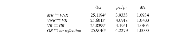
As summarised in table 2,
 ${\textit{MR}} \leftrightarrows {\textit{VNR}}$
denotes the transition criterion between Mach reflection and von Neumann reflection, which corresponds to the lower boundary of weak shock reflection domain,
 ${\textit{GR}} \leftrightarrows \textit{no}$
 $\textit{reflection}$
denotes the transition criterion between Guderley reflection and no reflection, which corresponds to the upper boundary of weak shock reflection domain,
 ${\textit{VNR}} \leftrightarrows {\textit{VR}}$
and
 ${\textit{VR}} \leftrightarrows {\textit{GR}}$
denote transition criteria from von Neumann reflection to Vasilev reflection and from Vasilev reflection to Guderley reflection, respectively, both of which are located in the weak shock reflection domain. These four criteria are very close. Therefore, we no longer further subdivide Type IIw shock interference based on the criteria in weak shock reflection.
The predicted boundaries between different reflection types at point
 $T_2$
(as shown in figure 5a) of Type II interference with
 $M_0=2.2$
.

Further, we display three Mach number contours for
 $M_0=2.2$
and
 $\theta _{01}=13^{\circ }$
with
 ${\textit{Ir}}=-4.9, -4.7 \textrm{ and } {-}4.3$
in figure 7. According to transition criteria presented in table 2, the wave configuration in these cases can be analysed.
Mach number contours at different
 ${\textit{Ir}}$
for
 $M_0=2.2$
and
 $\theta _{01}=13^{\circ }$
: (a)
 ${\textit{Ir}}=-4.9$
; (b)
 ${\textit{Ir}}=-4.7$
; (c)
 ${\textit{Ir}}=-4.3$
.

For
 ${\textit{Ir}}=-4.9$
, we extract
 $M_4=1.1224$
near point
 $T_2$
, along the incident shock of
 $T_2$
(as shown in figure 7a). By comparing with table 2, the flow near point
 $T_2$
is a Mach reflection. Figure 8(a) displays the shock polar of
 $T_2$
(the labels correspond to the labelled regions as shown in figure 5(a);
 $\varGamma _0$
denotes the shock polar with region (0) as the upstream,
 $\varGamma _4$
is defined similarly), further indicating that the flow near point
 $T_2$
is a Mach reflection. Thus, the interference type is Type II shock interference. For
 ${\textit{Ir}}=-4.3$
, the Mach number behind the bow shock is less than 1 (as shown in figure 7c), and only one triple point exist. This is a Type IIs shock interference. For
 ${\textit{Ir}}=-4.7$
, we extract
 $M_4=1.0671$
near point
 $T_2$
, along the incident shock of
 $T_2$
(as shown in figure 7b). By comparing with table 2, the flow near point
 $T_2$
has entered the weak shock reflection domain; specifically, it is a von Neumann reflection. Figure 8(b) displays the shock polar of
 $T_2$
, further indicating that the flow near point
 $T_2$
is a von Neumann reflection. The interference type is Type IIw shock interference.
Shock polars for triple point
 $T_2$
of cases with
 $M_0=2.2$
,
 $\theta _{01}=13^{\circ }$
: (a)
 ${\textit{Ir}}=-4.9$
; (b)
 ${\textit{Ir}}=-4.7$
.

The predicted boundaries between different reflection types at point
 $T_2$
(as shown in figure 5a) of Type II interference, when
 $M_0=2.5$
.

Similar phenomena can be observed when
 $M_0=2.5$
,
 $\theta _{01}=7.994^{\circ }$
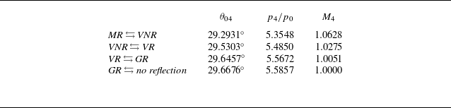
. Table 3 lists the predicted boundaries for the reflection at point
 $T_2$
. Figure 9 displays Mach number contours with
 ${\textit{Ir}}$
= −2.7, −2.51 and −2.31, and figure 10 displays shock polars of
 $T_2$
for
 ${\textit{Ir}}$
= −2.7 and −2.51. It can be seen that as
 ${\textit{Ir}}$
increases, interference types are Type II, Type IIw and Type IIs in sequence. In order to intuitively visualise the changes in reflection types of point
 $T_2$
, we display positions in the
 $M_0{-}\theta _{04}$
plane of parameters near point
 $T_2$
in figure 11: the grey area is weak shock reflection domain; the open circle denotes the case of
 $M_0=2.2$
,
 $\theta _{01}=13^{\circ }$
and
 ${\textit{Ir}}=-4.9$
; the solid circle denotes the case of
 $M_0=2.2$
,
 $\theta _{01}=13^{\circ }$
and
 ${\textit{Ir}}=-4.7$
; the open triangle denotes the case of
 $M_0=2.5$
,
 $\theta _{01}=7.994^{\circ }$
and
 ${\textit{Ir}}=-2.7$
; the solid triangles denote the case of
 $M_0=2.5$
,
 $\theta _{01}=7.994^{\circ }$
and
 ${\textit{Ir}}=-2.51$
.
Mach number contours at different
 ${\textit{Ir}}$
for
 $M_0=2.5$
and
 $\theta _{01}=7.994^{\circ }$
: (a)
 ${\textit{Ir}}=-2.7$
; (b)
 ${\textit{Ir}}=-2.51$
; (c)
 ${\textit{Ir}}=-2.41$
.

Shock polars for triple point
 $T_2$
of cases with
 $M_0=2.5$
,
 $\theta _{01}=7.994^{\circ }$
: (a)
 ${\textit{Ir}}=-2.7$
; (b)
 ${\textit{Ir}}=-2.51$
.

Positions in the
 $M_0-\theta _{04}$
plane of parameters near point
 $T_2$
.

Therefore, based on the evolution of triple point
 $T_2$
for Type II shock wave interference (as shown in figure 5a), we predict that there are new sub-types between Type II and Type III shock interference, and numerical results confirm two transitional sub-types, namely Type IIw (weak shock reflection at point
 $T_2$
) and Type IIs (no reflection at point
 $T_2$
, i.e.
 $T_2$
disappears).
3.2. The transition process between Type III and Type IV shock interference
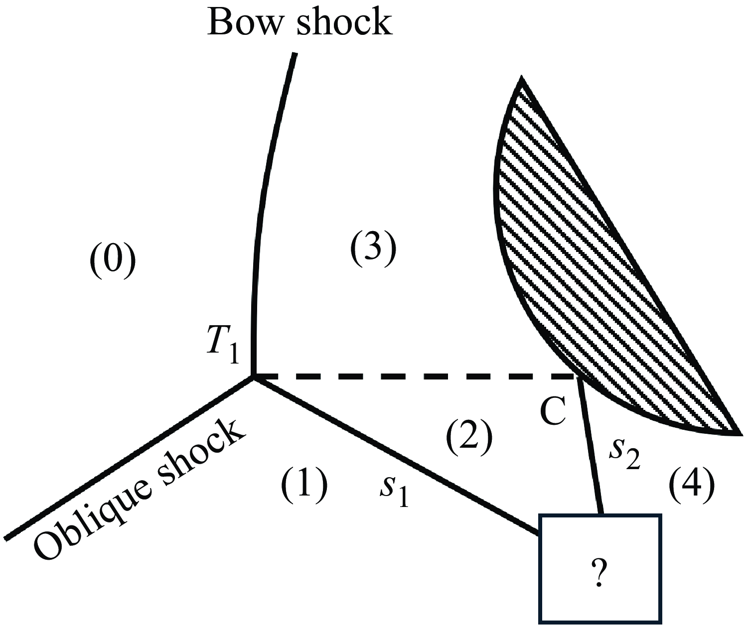
Type III interference has a crucial feature: the slipline is attached to the wall surface. As shown in figure 12, the oblique shock intersects with the bow shock, forming a triple point
 $T_1$
; the slipline
 $T_{1}C$
emanating from
 $T_1$
impacts on the blunt body surface and forms a shock
 $s_{2}$
, shock
 $s_{2}$
interferes with shock
 $s_1$
. If the interference between
 $s_1$
and
 $s_2$
changes, the wave configuration of Type III interference changes. Therefore, the interference between
 $s_1$
and
 $s_2$
is the key part of Type III interference.
Feature of Type III interference.

The flow from region (1) to (4), which forms shock
 $s_1$
through the first deflection and shock
 $s_2$
through the second deflection, can be regarded as a double-wedge shock interference, where the slipline acts as the first wedge and the blunt body acts as the second wedge.
Olejniczak, Wright & Candler (Reference Olejniczak, Wright and Candler1997) conducted a numerical study of double-wedge shock interference, and discovered five types of shock interference. Figure 13 shows the schematics for different types of shock interference for double wedge classified by Olejniczak et al. (Reference Olejniczak, Wright and Candler1997) (to avoid confusion, for the double-wedge shock interference types discovered by Olejniczak et al., we add the prefix ‘Olejniczak’).
-
(i) Olejniczak Type VI: the wave configuration is the same as Type VI interference, as shown in figure 13(a).
-
(ii) Olejniczak Type I: compared with Olejniczak Type VI interference, a shock replaces the expansion wave, as shown in figure 13(b).
-
(iii) Olejniczak Type V: the wave configuration is the same as Type V interference, as shown in figure 13(c).
-
(iv) Olejniczak Type IV: the wave configuration is the same as Type IV interference, as shown in figure 13(d)
-
(v) Olejniczak Type IVr: the wave configuration consists of a triple points and a jet, as shown in figure 13(e).
Schematics of shock interference on double-wedge geometries: (a) Olejniczak Type VI; (b) Olejniczak Type I; (c) Olejniczak Type V; (d) Olejniczak Type IV; (e) Olejniczak Type IVr.

Olejniczak et al. (Reference Olejniczak, Wright and Candler1997) also proposed transition criteria through numerical simulations and theoretical analyses, the transition criterion between Olejniczak Type V and Olejniczak Type VI are applicable between Type V and Type VI. Furthermore, if the first wedge angle is constant, then: when the incoming flow Mach number
 $M_0$
is small, as the second wedge angle increases, the shock interference evolves in the order of Olejniczak Type VI, I, V and IV; when the incoming flow Mach number
 $M_0$
is large, as the second wedge angle increases, the shock interference evolves in the order of Olejniczak Type VI, V, IV and IVr.
With reference to the evolution of double-wedge shock interference, the interference between
 $s_1$
and
 $s_2$
(as shown in figure 12) should also exhibit multiple configurations, which means that Type III interference has other new sub-types.
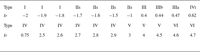
We select several cases with
 $M_0=5$
and
 $\theta _{01}=17^{\circ }$
for numerical simulation to validate our assumption, and Mach number contours are shown in figure 14. The interference between shocks
 $s_1$
and
 $s_2$
evolves in the order of Olejniczak Type VI, I, V and IV as
 ${\textit{Ir}}$
increases from 0.4 to 0.62.
-
(i) For
 ${\textit{Ir}}=0.4$
, the interference between shocks
$s_1$
and
$s_2$
seems to be a triple point, as shown in figure 14(a). However, the shock polar diagram for the interference between
$s_1$
and
$s_2$
as shown in figure 16 reveals a different scenario (the labelled points in the shock polar diagram correspond to the labelled regions as shown in figure 5(b);
$\varGamma _1$
denotes the shock polar with region (1) as the upstream,
$\varGamma _3$
is defined similarly;
$\varGamma _4$
denotes the expansion wave polar with region (4) as the upstream). We find that the interference between the shock waves
$s_1$
and
$s_2$
is an Olejniczak Type VI interference accompanied by a weak expansion wave (the flow deflection angle is only
$0.0505^{\circ }$
). Since the flow is highly inhomogeneous in this region and numerous waves are coupled together, this weak expansion wave is difficult to directly distinguish from other waves. Thus, the actual wave configuration is a Type III shock interference.
-
(ii) For
${\textit{Ir}}=0.44$
, as shown in figure 14(b), the interference between shocks
$s_1$
and
$s_2$
corresponds to the configuration shown in figure 13(b). We name this wave configuration as Type IIIb shock interference, the schematic is displayed in figure 15(a). -
(iii) For
${\textit{Ir}}=0.47$
, as shown in figure 14(c), the interference between shocks
$s_1$
and
$s_2$
corresponds to the configuration shown in figure 13(c). Peng et al. (Reference Peng, Li, Yang, Lin, Han and Hu2023) classified this wave configuration as Type IIIa shock interference, the schematic is displayed in figure 15(b). -
(iv) For
${\textit{Ir}}=0.62$
, as shown in figure 14(d), the interference between shock
$s_1$
and shock
$s_2$
corresponds to the configuration shown in figure 13(d). Since shock
$s_1$
is detached and the slipline is no longer attached to the wall, we consider this wave configuration as the termination of Type III interference and the initiation of Type IV interference, and name this wave configuration as Type IVt shock interference. The schematic is displayed in figure 15(c). -
(v) For
${\textit{Ir}}=0.75$
, as shown in figure 14(e), the wave configuration is a Type IV shock interference.


Mach number contours at different
 ${\textit{Ir}}$
for
 $M_0=5$
and
 $\theta _{01}=17^{\circ }$
: (a)
 ${\textit{Ir}}=0.4$
; (b)
 ${\textit{Ir}}=0.44$
; (c)
 ${\textit{Ir}}=0.47$
; (d)
 ${\textit{Ir}}=0.62$
; (e)
 ${\textit{Ir}}=0.75$
.

Schematics for transitional types of shock interferences between Type III and Type IV interferences: (a) Type IIIb; (b) Type IIIa; (c) Type IVt.

Shock polar for the case with
 $M_0=5$
,
 $\theta _{01}=17^{\circ }$
and
 ${\textit{Ir}}=0.4$
: (a) polar curve; (b) enlarged view.

Therefore, based on the analogy of the interference between shocks
 $s_1$
and
 $s_2$
(as shown in figure 12) to double-wedge shock wave interference, we have found that there are three transitional sub-types between Type III and Type IV shock wave interference, namely Type IIIb (the interference between shocks
 $s_1$
and
 $s_2$
is an Olejniczak Type I interference) , Type IIIa (the interference between shocks
 $s_1$
and
 $s_2$
is an Olejniczak Type V interference) and Type IVt (the interference between shocks
 $s_1$
and
 $s_2$
is an Olejniczak Type IV interference).
3.3. The transition process between Type IV and Type V shock interference
The wave configuration of Type IV shock interference is displayed in figure 17(a). The oblique shock intersects with the bow shock, resulting in two triple points
 $T_1$
and
 $T_2$
: the first triple point
 $T_1$
corresponds to a Mach reflection, where the oblique shock is the incident shock, the bow shock above triple point
 $T_1$
is the Mach stem, shock
 $T_{1}T_{2}$
is the reflected shock; the second triple point
 $T_2$
corresponds to a Mach reflection, where shock
 $T_{1}T_{2}$
is the incident shock, the bow shock below triple point
 $T_{2}$
is the Mach stem. The region between the sliplines of two triple points is a jet. The wave configuration of Type V shock interference is displayed in figure 17(b). The oblique shock intersects with the bow shock, resulting in three triple points
 $T_1$
,
 $T_2$
and
 $T_3$
, the wave configuration in the vicinity of
 $T_1$
and
 $T_2$
is similar to Type IV interference, and the wave configuration at point
 $T_3$
corresponds to a Mach reflection, where the bow shock is the incident shock.
Schematics of Type IV and Type V shock interferences.

The difference between Type IV and Type V interference is whether the triple point
 $T_3$
exists. Therefore, the transition process between Type IV and Type V interference is determined by the evolution of the reflection at point
 $T_3$
, it is similar as the transition process between Type II and Type IIs shock interference.
For incoming flow Mach number
 $M_0$
and
 $\theta _{01}$
,
 $M_1$
is determined. With the increase of
 ${\textit{Ir}}$
, the position of triple point
 $T_3$
increase along the bow shock, where the bow shock is the incident shock of
 $T_3$
. The rise in the position of point
 $T_3$
means that the flow deflection angle
 $\theta _{16}$
of the incident shock at the point
 $T_3$
increases. In
 $\S$
2.1, the transition criteria between different types of shock reflection are given. If the flow deflection angle
 $\theta _{16}$
enters the weak shock reflection domain, the wave configuration near point
 $T_3$
transits to weak shock reflection, which means that Type V shock interference transits to a new type, which we name as Type Vw shock interference. Then, we select a specific case to further validate this new type.
For
 $M_0=5$
and
 $\theta _{01}=25^{\circ }$
, we obtain
 $M_1=2.5658$
, which is the incoming flow Mach number for point
 $T_3$
. We use the method introduced in
 $\S$
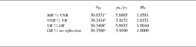
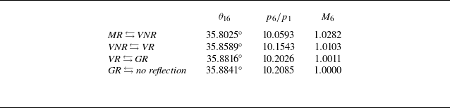
2.1 to obtain predicted boundaries between different reflection types. Then, we can obtain the corresponding
 $M_6$
and
 $p_{6}/p_{1}$
. These predicted boundaries are summarised in table 4.
The predicted boundaries between different reflection types at point
 $T_3$
(as shown in figure 17b) of Type V interference, when
 $M_1=2.5658$
.

Further, we display three Mach number contours for
 $M_0=5$
and
 $\theta _{01}=25^{\circ }$
with
 ${\textit{Ir}}=4.75, 4.87, 5$
in figure 18. According to the transition criteria given in table 4, the wave configuration in these cases can be analysed.
Mach number contours at different
 ${\textit{Ir}}$
for
 $M_0=5$
and
 $\theta _{01}=25^{\circ }$
: (a)
 ${\textit{Ir}}=4.75$
; (b)
 ${\textit{Ir}}=4.87$
; (c)
 ${\textit{Ir}}=5$
.

For
 ${\textit{Ir}}=5$
, we extract
 $M_4=1.1538$
near point
 $T_3$
, along the incident shock of
 $T_3$
. By comparing with table 4, the flow near point
 $T_3$
is a Mach reflection. Figure 19(a) display the shock polar of
 $T_3$
(the labels correspond to the labelled regions as shown in figure 17(b);
 $\varGamma _1$
denotes the shock polar with region (1) as the upstream;
 $\varGamma _6$
is defined similarly), it further indicates that the flow near point
 $T_3$
is a Mach reflection. Thus, the interference type is Type V shock interference. For
 ${\textit{Ir}}=4.75$
, the Mach number behind the bow shock is less than 1, and only one triple point exist. This is a Type IV shock interference. For
 ${\textit{Ir}}=-4.87$
, we extract
 $M_6=1.0439$
near point
 $T_3$
, along the incident shock of
 $T_3$
. By comparing with table 4, the flow near point
 $T_3$
has entered the weak shock reflection domain, specifically, it is a von Neumann reflection. Figure 19(b) display the shock polar of
 $T_3$
, it further indicates that the flow near point
 $T_3$
is a von Neumann reflection. Thus, the interference type is Type Vw shock interference. In order to intuitively visualise the changes in reflection types of point
 $T_3$
, we display positions in the
 $M_1-\theta _{16}$
plane of parameters near point
 $T_3$
in figure 20: the grey area is weak shock reflection domain; open circle denotes the case of
 $M_0=5$
,
 $\theta _{01}=25^{\circ }$
and
 ${\textit{Ir}}=5$
; the solid circle denotes the case of
 $M_0=5$
,
 $\theta _{01}=25^{\circ }$
and
 ${\textit{Ir}}=4.87$
.
Shock polars for triple point
 $T_3$
of cases with
 $M_0=5$
,
 $\theta _{01}=25^{\circ }$
: (a)
 ${\textit{Ir}}=4.87$
; (b)
 ${\textit{Ir}}=5$
.

Positions in the
 $M_1-\theta _{16}$
plane of parameters near point
 $T_3$
.

Therefore, based on the evolution of triple point
 $T_3$
for Type V shock wave interference (as shown in figure 17b), we predict that there is a new sub-type between Type IV and Type V shock interference, and numerical results confirm this transitional sub-types, namely Type Vw (weak shock reflection at point
 $T_2$
).
4. Global research on six types of shock interference
In this section, we conduct a more comprehensive investigation on the evolution of shock interference within a broader parameter range. Four distinct combinations of
 $M_0$
and
 $\theta _{01}$
are selected for simulation, specifically,
 $M_0=2.5$
with
 $\theta _{01}=7.994^\circ$
,
 $M_0=2.5$
with
 $\theta _{01}=17^\circ$
,
 $M_0=5$
with
 $\theta _{01}=17^\circ$
and
 $M_0=5$
with
 $\theta _{01}=25^\circ$
. For each combination, we investigate the corresponding transition processes from Type I to Type VI shock interference by varying
 ${\textit{Ir}}$
. A total of 12 types of shock interference are observed.
4.1. The evolution of shock interference under
$M_0=2.5$
and
$\theta _{01}=7.994^\circ$


For
 $M_0=2.5$
and
 $\theta _{01}=7.994^\circ$
, we select 18 cases with different
 ${\textit{Ir}}$
for numerical simulation. Figure 21 presents Mach number contours for some representative cases, the variation of the shock interference type with
 ${\textit{Ir}}$
is summarised as follows.
-
(i) For
${\textit{Ir}}$
= −3.5, −2.7 and −2.51, the wave configurations correspond to Type I, Type II and Type IIw, respectively. -
(ii) For
${\textit{Ir}}$
= 0, 1, 1.1, 1.2, 1.5, 2 and 4, the wave configurations remain Type IIs, even when the slipline is located above the blunt body. The reason for these phenomena is that the flow below the slipline is subsonic, and it is indicated that Type III and Type IV shock interferences do not exist. It can be observed that the shape of the slipline changes. When
${\textit{Ir}}= 0$
and 1, the slipline deflects downwards. When
${\textit{Ir}}$
= 1.1, 1.2 and 1.5, the slipline first deflects downwards and then upwards. With the increase of
${\textit{Ir}}$
, the portion of the slipline that deflects downwards is getting shorter. When
${\textit{Ir}}$
= 4, the portion of the slipline that deflects downwards is virtually unobservable. -
(iii) For
${\textit{Ir}}=4.3$
, a new triple point occurs. It is similar as Type V interference without the triple point
$T_2$
, the reason is that the flow below the slipline originating from
$T_1$
is subsonic. We classify it as Type Va interference, figure 22 shows a schematic. -
(iv) For
${\textit{Ir}}=5$
, the wave configuration is Type VI interference.


Mach number contours at different
 ${\textit{Ir}}$
for
 $M_0=2.5$
and
 $\theta _{01}=7.994^{\circ }$
: (a)
 ${\textit{Ir}}=-3.5$
; (b)
 ${\textit{Ir}}=-2.7$
; (c)
 ${\textit{Ir}}=-2.51$
; (d)
 ${\textit{Ir}}=0$
; (e)
 ${\textit{Ir}}=1$
; (f)
 ${\textit{Ir}}=1.1$
; (g)
 ${\textit{Ir}}=1.2$
; (h)
 ${\textit{Ir}}=1.5$
; (i)
 ${\textit{Ir}}=2$
; (j)
 ${\textit{Ir}}=4$
; (k)
 ${\textit{Ir}}=4.3$
; (l)
 ${\textit{Ir}}=5$
.

Schematic of Type Va shock interference.

Table 5 summarises the types of shock interference for all 18 cases with different
 ${\textit{Ir}}$
. It can be observed that as
 ${\textit{Ir}}$
increases, the shock interference does not change step by step in the order of Type I
 $\rightarrow$
Type II
 $\rightarrow$
Type III
 $\rightarrow$
Type IV
 $\rightarrow$
Type V
 $\rightarrow$
Type VI, even classical Type III, Type IV and Type V interferences do not exist. In fact, the entire transition sequence of shock interference is Type I
 $\rightarrow$
Type II
 $\rightarrow$
Type IIw
 $\rightarrow$
Type IIs
 $\rightarrow$
Type Va
 $\rightarrow$
Type VI.
4.2. The evolution of shock interference under
$M_0=2.5$
and
$\theta _{01}=17^\circ$


For
 $M_0=2.5$
and
 $\theta _{01}=17^\circ$
, we select 18 cases with different
 ${\textit{Ir}}$
for numerical simulation. Figure 23 presents the Mach number contours for some representative cases, the variation of the shock interference type with
 ${\textit{Ir}}$
is summarised as follows.
-
(i) For
${\textit{Ir}}$
= −9.2, −6, −4 and −2, the wave configurations correspond to Type I, Type II, Type IIw and Type IIs, respectively. -
(ii) For
${\textit{Ir}}$
= 2, 3 and 6, the wave configurations are still Type IIs, but the slipline has impacted on the blunt body and even the slipline is located above the blunt body. It can be observed that the shape of the slipline changes with
${\textit{Ir}}$
. -
(iii) For
${\textit{Ir}}$
= 10 and 12, the wave configurations correspond to Type Va and Type VI, respectively.


Mach number contours at different
 ${\textit{Ir}}$
for
 $M_0=2.5$
and
 $\theta _{01}=17^{\circ }$
: (a)
 ${\textit{Ir}}=-9.2$
; (b)
 ${\textit{Ir}}=-6$
; (c)
 ${\textit{Ir}}=-4$
; (d)
 ${\textit{Ir}}=-2$
; (e)
 ${\textit{Ir}}=0$
; (f)
 ${\textit{Ir}}=1$
; (g)
 ${\textit{Ir}}=2$
; (h)
 ${\textit{Ir}}=3$
; (i)
 ${\textit{Ir}}=6$
; (j)
 ${\textit{Ir}}=10$
; (k)
 ${\textit{Ir}}=12$
.

The types of shock interference under different
 ${\textit{Ir}}$
(
 $M_0=2.5$
,
 $\theta _{01}=7.994^{\circ }$
).

The transition process is similar to that for
 $M_0=2.5$
and
 $\theta _{01}=7.994^\circ$
. However, there is a difference. For the cases under
 $M_0=2.5$
and
 $\theta _{01}=7.994^\circ$
, the reason for the non-existence of Type III and Type IV interference is that the flow below the slipline is subsonic. However, for
 $M_0=2.5$
and
 $\theta _{01}=17^\circ$
, in the vicinity of the triple point of Type IIs interference, we can obtain the flow in region (2) behind the reflected shock is supersonic through the three-shock theory.
Enlarged views of Mach number contours with
 ${\textit{Ir}}$
= −2, 0, 1 and 2 are shown in figure 24. For
 ${\textit{Ir}}=-2$
, the flow below the slipline is all supersonic. As
 ${\textit{Ir}}$
increases, the subsonic region emerges whereas the supersonic region gradually shrinks. For
 ${\textit{Ir}}=2$
, below the slipline, the Mach number gradually decreases along the flow direction, and the flow transitions from supersonic to subsonic, such that no new shock is formed at the wall. The reason for this phenomenon is that the flow above the slipline gradually decelerates as it moves towards the wall and eventually stagnates, causing a pressure increase. To maintain pressure balance across the slipline, the pressure below the slipline also rises accordingly, leading to a decrease in the Mach number.
Enlarged view of Mach number contours for
 $M_0=2.5$
and
 $\theta _{01}=17^{\circ }$
: (a)
 ${\textit{Ir}}=2$
; (b)
 ${\textit{Ir}}=0$
; (c)
 ${\textit{Ir}}=1$
; (d)
 ${\textit{Ir}}=-2$
.

Table 6 summarises the types of shock interference for all 18 cases with different
 ${\textit{Ir}}$
. The entire transition process of shock interference is Type I
 $\rightarrow$
Type II
 $\rightarrow$
Type IIw
 $\rightarrow$
Type IIs
 $\rightarrow$
Type Va
 $\rightarrow$
Type VI, and Type III, Type IV and Type V interferences do not exist.
The types of shock interference under different
 ${\textit{Ir}}$
(
 $M_0=2.5$
,
 $\theta _{01}=17^{\circ }$
).

4.3. The evolution of shock interference under
$M_0=5$
and
$\theta _{01}=17^\circ$


For
 $M_0=5$
and
 $\theta _{01}=17^\circ$
, we select 22 cases with different
 ${\textit{Ir}}$
for numerical simulation. Figure 25 presents Mach number contours for some representative cases, the variation of the shock interference type with
 ${\textit{Ir}}$
is summarised as follows.
-
(i) For
${\textit{Ir}}$
= −2 and −1, the wave configurations respectively correspond to Type I and Type IIs, respectively. -
(ii) For
${\textit{Ir}}$
= 0.4, 0.44, 0.47, 0.62 and 0.75, the wave configurations correspond to Type III, Type IIIb, Type IIIa, Type IVt and Type IV, respectively. -
(iii) For
${\textit{Ir}}$
= 2.5 and 2.9, the wave configurations are still Type IV. -
(iv) For
${\textit{Ir}}$
= 3 and 4.6, the wave configurations correspond to Type V and Type VI, respectively.


Mach number contours at different
 ${\textit{Ir}}$
for
 $M_0=5$
and
 $\theta _{01}=17^{\circ }$
: (a)
 ${\textit{Ir}}=-2$
; (b)
 ${\textit{Ir}}=-1$
; (c)
 ${\textit{Ir}}=0.4$
; (d)
 ${\textit{Ir}}=0.44$
; (e)
 ${\textit{Ir}}=0.47$
; (f)
 ${\textit{Ir}}=0.62$
; (g)
 ${\textit{Ir}}=0.75$
; (h)
 ${\textit{Ir}}=2.5$
; (i)
 ${\textit{Ir}}=2.9$
; (j)
 ${\textit{Ir}}=3$
; (k)
 ${\textit{Ir}}=4.6$
.

Type II, Type IIw and Type Vw interferences are not observed. For Type V interference, the Mach number
 $M_1$
= 3.3088 (as shown in figure 17b). Table 8 presents the predicted boundaries for different types of the reflection at triple point
 $T_3$
of Type V interference when
 $M_1$
= 3.3088. According to § 3.3, Type Vw interference occurs when the reflection at point
 $T_3$
transit to weak shock reflection. Therefore, Type Vw interference occurs when
 $M_6$
range from 1 to 1.028, this small range makes it difficult to observe Type Vw interference. However, the absence of observation of Type II and Type IIw is yet to be clarified.
Table 7 summarises the types of shock interference for all 22 cases with different
 ${\textit{Ir}}$
. The entire transition process of shock interference is Type I
 $\rightarrow$
Type IIs
 $\rightarrow$
Type III
 $\rightarrow$
Type IIIb
 $\rightarrow$
Type IIIa
 $\rightarrow$
Type IVt
 $\rightarrow$
Type IV
 $\rightarrow$
Type V
 $\rightarrow$
Type VI, and Type II, Type IIw and Type Vw interferences are not observed.
The types of shock interference under different
 ${\textit{Ir}}$
(
 $M_0=5$
,
 $\theta _{01}=17^{\circ }$
).

The predicted boundaries between different reflection types at point
 $T_3$
(as shown in figure 17b) of Type V interference, when
 $M_1=3.3088$
.

4.4. The evolution of shock interference under
$M_0=5$
and
$\theta _{01}=25^\circ$


For
 $M_0=5$
and
 $\theta _{01}=25^\circ$
, we select 30 cases with different
 ${\textit{Ir}}$
for numerical simulation. Figure 26 presents the Mach number contours for some representative cases, the variation of the shock interference type with
 ${\textit{Ir}}$
is summarised as follows.
-
(i) For
${\textit{Ir}}$
= −4.5, −3.4, 0.75 and 0.82, the wave configurations respectively correspond to Type I, Type IIs, Type III and Type IIIb, respectively. -
(ii) For
${\textit{Ir}}$
= 0.83 and 0.9, two strange wave configurations are observed, their schematics are displayed in figure 27. Compared with Type IIIa and Type IVt interference, both of them lack a triple point
$T_3$
. This phenomenon is analysed. -
(iii) For
${\textit{Ir}}=1.5$
, the wave configuration is a Type IVt interference. An enlarged view of the Mach number contour is shown in figure 28, where a triple point
$T_3$
and a triangular region (5) appear (corresponding to figure 15c). -
(iv) For
${\textit{Ir}}$
= 2.51 and 4.75, the wave configurations are all Type IV interference. -
(v) For
${\textit{Ir}}$
= 4.87 and 5, the wave configurations respectively correspond to Type Vw and Type V shock interferences. -
(vi) For
${\textit{Ir}}= 8$
, the wave configuration is Type VI shock interference.


Mach number contours at different
 ${\textit{Ir}}$
for
 $M_0=5$
and
 $\theta _{01}=25^{\circ }$
: (a)
 ${\textit{Ir}}=-4.5$
; (b)
 ${\textit{Ir}}=-3.4$
; (c)
 ${\textit{Ir}}=0.75$
; (d)
 ${\textit{Ir}}=0.82$
; (e)
 ${\textit{Ir}}=0.83$
; (f)
 ${\textit{Ir}}=0.9$
; (g)
 ${\textit{Ir}}=1.5$
; (h)
 ${\textit{Ir}}=2.51$
; (i)
 ${\textit{Ir}}=4.75$
; (j)
 ${\textit{Ir}}=4.87$
; (k)
 ${\textit{Ir}}=5$
; (l)
 ${\textit{Ir}}=8$
.

Figure 29 displays the Mach number and pressure contours with
 ${\textit{Ir}}=0.83$
, figure 30 displays the Mach number and pressure contours with
 ${\textit{Ir}} = 0.9$
. The regions marked (5) in both figures 27(a) and 27(b) are subsonic. However, we use the three-shock theory to analyse these regions, and find that they should be supersonic. Pressure contours in figures 29 and 30 indicate that pressure vary significantly downstream of point
 $T_2$
. The inapplicability of the three-shock theory and the sharp variation in pressure indicate that the point
 $T_2$
is not a triple point, but a more complex unknown configuration. In additional, a triple point
 $T_3$
and a triangular region (5) corresponding to figure 15(c) appear when
 ${\textit{Ir}} = 1.5$
. Therefore, we speculate that the wave configuration is Type IIIa when
 ${\textit{Ir}}=0.83$
, and the wave configuration is Type IVt when
 ${\textit{Ir}}$
= 0.9. However, the close proximity of
 $T_2$
and
 $T_3$
combined with the extremely small size of the triangle make these configurations difficult to observe.
Schematics for the wave configuration with: (a)
 ${\textit{Ir}}$
= 0.83; (b)
 ${\textit{Ir}}$
= 0.9.

Enlarged view of the Mach number contour when
 $M_0=5$
,
 $\theta _{01}=25^{\circ }$
and
 ${\textit{Ir}}=1.5$
.

Enlarged view of the flow structure when
 $M_0=5$
,
 $\theta _{01}=25^{\circ }$
and
 ${\textit{Ir}}=0.83$
: (a) enlarged view of the Mach number contour; (b) enlarged view of the pressure contour (
 $p/p_0$
).

Enlarged view of the flow structure when
 $M_0=5$
,
 $\theta _{01}=25^{\circ }$
and
 ${\textit{Ir}}=0.9$
: (a) enlarged view of the Mach number contour; (b) enlarged view of the pressure contour (
 $p/p_0$
).

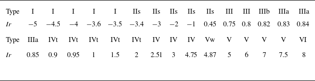
Table 9 summarises the types of shock interference for all 30 cases with different
 ${\textit{Ir}}$
. The entire transition process of shock interference is Type I
 $\rightarrow$
Type IIs
 $\rightarrow$
Type III
 $\rightarrow$
Type IIIb
 $\rightarrow$
Type IIIa
 $\rightarrow$
Type IVt
 $\rightarrow$
Type IV
 $\rightarrow$
Type V
 $\rightarrow$
Type Vw
 $\rightarrow$
Type VI, and Type II and Type IIw interferences are not observed, similar to the situation with
 $M_0=5$
and
 $\theta _{01}=25^\circ$
.
4.5. Summary
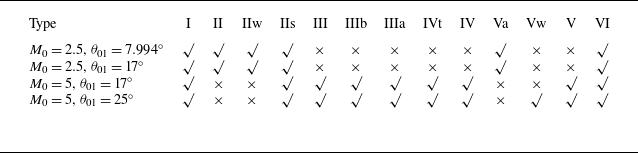
Table 10 summarises the types of shock interference under different
 $M_0$
and
 $\theta _{01}$
. It reveals the significant influence of incoming flow Mach number on the types of shock interference. Under large incoming flow Mach number (for example,
 $M_0=5$
), Type III, Type IV and their related sub-types (Type IIIb, Type IIIa and Type IVt) are more likely to occur, whereas Type II interference is absent, the transition sequence is Type I
 $\rightarrow$
Type IIs
 $\rightarrow$
Type III
 $\rightarrow$
Type IIIb
 $\rightarrow$
Type IIIa
 $\rightarrow$
Type IVt
 $\rightarrow$
Type IV
 $\rightarrow$
Type V
 $\rightarrow$
Type Vw
 $\rightarrow$
Type VI. Since our numerical calculations can only select
 ${\textit{Ir}}$
discretely, Type II and Type IIw may not truly be non-existent under the conditions of
 $M_0=5$
,
 $\theta _{01}=17^{\circ }$
and
 $M_0=5$
,
 $\theta _{01}=25^{\circ }$
. However, due to the interval of 0.1 for the selected
 ${\textit{Ir}}$
between Type I and Type IIs, it can at least indicate that the existence range of Type II and Type IIw is very small under the above two operating conditions.
In contrast, under small incoming flow Mach number (for example,
 $M_0=2.5$
), Type IV, Type III and Type V do not appear. Instead, Type Va interference emerges, characterised by the absence of a triple point compared with Type V interference. The transition sequence is Type I
 $\rightarrow$
Type II
 $\rightarrow$
Type IIw
 $\rightarrow$
Type IIs
 $\rightarrow$
Type Va
 $\rightarrow$
Type VI.
This study identifies seven sub-types that extend the classical six types of shock interferences into six-plus shock interference, establishing a complete and continuous chain for the evolution of shock interferences. Figure 31 presents a schematic diagram of the six typical shock interferences and the new sub-types. The reflection type of triple point
 $T_2$
of Type II is a Mach reflection (denoted as
 ${\textit{MR}}$
in figure 31); when its position shifts upwards, leading to a transition of the reflection type to a weak shock reflection (denoted as
 $ \textit{WR} $
in figure 31), Type IIw occurs. When point
 $T_2$
of Type IIw lies at the sonic point of the bow shock, the reflection here disappears, and Type IIs occurs. As
 ${\textit{Ir}}$
increases to the point where the slip line of Type IIs attaches to the wall, Type III occurs. An increase in
 ${\textit{Ir}}$
alters the intensities of shocks
 $s_1$
and
 $s_2$
in Type III, thereby inducing a change in the interference type, with Type IIIb and Type IIIa appearing sequentially. Type IIIa was first identified and named by Peng et al. (Reference Peng, Li, Yang, Lin, Han and Hu2023). When shock
 $s_2$
at point
 $C$
of Type IIIa detaches, the slipline is no longer attached to the wall, and Type IVt occurs. The transition between Type IV and Type V is similar to that between Type II and Type III: the reflection type of triple point
 $T_3$
of Type V is a Mach reflection; when its position shifts downwards, causing the reflection type to switch to a weak shock reflection, Type Vw occurs. When point
 $T_3$
of Type Vw lies at the sonic point of the bow shock, the reflection here disappears, and Type IV occurs. In addition, Type V has an exceptional sub-type: when the flow behind the reflected shock at point
 $T_1$
of Type V is subsonic, point
 $T_2$
does not exist, and Type Va occurs.
Six-plus shock interference patterns, with Edney six types of shock interferences and sub-types between Type II and Type III, Type III and Type IV, and Type IV and Type V shock interferences.

The types of shock interference under different
 ${\textit{Ir}}$
(
 $M_0=5$
,
 $\theta _{01}=25^{\circ }$
).

The types of shock interference under different
 $M_0$
and
 $\theta _{01}$
.

5. Conclusion
This study has systematically investigated the transition processes between six types of shock interferences defined by Edney (Reference Edney1968) (Type I to Type VI). The key findings of this research are summarised as follows.
First, the discovery of new interference sub-types based on the evolution of triple points. Between Type II and Type III shock interference, Type IIw and Type IIs are obtained. Type IIw occurs when the flow near the triple point of Type II enters weak shock reflection; Type IIs occurs when the triple point of Type II disappears. Between Type IV and V shock interference, Type Vw is obtained. Type Vw occurs when the flow near the triple point of Type V enters the weak shock reflection domain.
Second, the discovery of new interference sub-types based on the analogy of double-wedge shock interference. Regarding the partial configuration of Type III shock interference as double-wedge shock interference problems, it was found that in addition to the previously reported Type IIIa, Type IIIb and Type IVt were also recorded and verified through numerical simulations.
Third, global research on the evolution of shock interference. It is revealed that the incoming flow Mach number has a significant influence on the types of shock interference. Under large incoming flow Mach number (for example,
 $M_0=5$
), Type III, Type IV and their related sub-types (Type IIIb, Type IIIa and Type IVt) are more likely to occur, whereas Type II interference is absent. In contrast, under small incoming flow Mach number (for example,
 $M_0=2.5$
), Type IV, Type III and Type V do not appear. Instead, Type Va interference emerges, characterised by the absence of a triple point compared with Type V interference.
In general, this work improves the classical Edney classification. The newly discovered types collectively form a continuous evolutionary chain of shock interferences. These results provide deeper physical insights into the complex mechanisms of shock wave interference transitions, forming a more complete framework for future theoretical and applied research in high-speed aerodynamics.
Acknowledgements
The authors are grateful to all referees for their useful comments and references, which helped improve the manuscript. This work was supported by the National Natural Science Foundation of China (nos 12472232 and 52192632) and Beihang University Young Elite Talent Support Program (501XYGG2025105003).
Declaration of interests
The authors have no conflicts of interest to report.
Appendix A. Three-shock theory
In this appendix we introduce three-shock theory for solving the flow parameters in the vicinity of a triple point.
First, we need to review the oblique shock relations. Through the oblique shock relations
 \begin{equation} \left \{ \!\!\begin{array}{l} \theta _{ud}=f_{\theta }(M_{u},\beta _{ud}), \\ M_{d}=f_{m}(M_{u},\beta _{ud}), \\ p_{d}/p_{u}=f_{p}(M_{u},\beta _{ud}),\end{array}\right . \end{equation}
where
 \begin{equation} \left \{ \!\!\begin{array}{l} f_{\theta }(M_{u},\beta _{ud})=\arctan \left \{ 2\cot \beta _{ud}\dfrac {M_{u}^{2}\mathrm{sin}^{2}\beta _{ud}-1}{M_{u}^{2}(\gamma +\cos 2\beta _{ud})+2}\right \} ,\\[8pt] f_{m}(M_{u},\beta _{ud})=\sqrt {\dfrac {M_{ud}^{2}+\dfrac {2}{\gamma -1}}{\dfrac {2\gamma }{\gamma -1}M_{ud}^{2}\mathrm{sin}^{2}\beta _{ud}-1}+\dfrac {M_{ud}^{2}\mathrm{cos}^{2}\beta _{d}}{\dfrac {\gamma -1}{2}M_{ud}^{2}\mathrm{sin}^{2}\beta _{ud}+1}} ,\\[8pt] f_{p}(M_{u},\beta _{ud})=1+\dfrac {2\gamma }{\gamma +1}(M_{ud}^{2}\mathrm{sin}^{2}\beta _{ud}-1),\end{array}\right . \end{equation}
the shock angle
 $\beta _{ud}$
is related to the flow deflection angle
 $\theta _{ud}$
and the Mach number
 $M_{u}$
in upstream flow, the pressure ratio between downstream and upstream is related to the shock angle
 $\beta _{ud}$
and the Mach number
 $M_{u}$
in upstream flow and the Mach number
 $M_{d}$
in the downstream flow is related to the shock angle
 $\beta _{ud}$
and the Mach number
 $M_{u}$
in upstream flow. The three-shock theory was proposed by von Neumann (Reference von Neumann1945) for describing the flow near a triple point. Figure 2(a) shows the schematic of a triple point for Mach reflection, which includes an incident shock
 $i$
, a reflected shock
 $r$
, a Mach stem
 $m$
and a slipline
 $s$
. These structures divide the flow field into four regions (0) to (3). Based on the oblique shock relations, the relationships of flow parameters between region (0) and region (1), region (0) and region (3), and region (1) and region (2) satisfy
 \begin{align}& \left \{ \!\!\begin{array}{l} \theta _{01}=f_{\theta }(M_{0},\beta _{01}) ,\\ M_1=f_m(M_0,\beta _{01}) ,\\ p_1/p_0=f_p(M_0,\beta _{01}), \end{array}\right . \end{align}
 \begin{align}& \left \{ \!\!\begin{array}{l} \theta _{12}=f_{\theta }(M_{1},\beta _{12}) ,\\ M_2=f_m(M_1,\beta _{12}), \\ p_2/p_1=f_p(M_1,\beta _{12}), \end{array}\right . \end{align}
 \begin{align}& \left \{ \!\!\begin{array}{l} \theta _{03}=f_{\theta }(M_{0},\beta _{03}) ,\\ M_{3}=f_{m}(M_{0},\beta _{03}) ,\\ p_{3}/p_{0}=f_{p}(M_{0},\beta _{03}).\end{array}\right . \end{align}
The flow satisfies the following conditions: the pressure balance condition (the pressures behind the reflected shock and the Mach stem are balanced) and flow parallel condition (the flow directions on both sides of the slipline are parallel). Thus, the following equations are obtained:
 \begin{equation} \left \{\!\! \begin{array}{l} p_{2}=p_{3}, \\ \theta _{03}=\theta _{01} \pm \theta _{12},\end{array}\right . \end{equation}
where
 $\theta _{03}=\theta _{01}{-}\theta _{12}$
when the flow deflects upwards after passing through the reflected shock, as shown in figure 2(a);
 $\theta _{03}=\theta _{01}+\theta _{12}$
when the flow deflects downwards after passing through the reflected shock, as shown in figure 2(b).
Given the flow parameters
 $M_0$
,
 $\theta _{01}$
and
 $\gamma$
, the flow parameters
 $\theta _{03}$
,
 $\theta _{12}$
,
 $\beta _{01}$
,
 $\beta _{03}$
,
 $\beta _{12}$
,
 $p_{1}/p_{0}$
,
 $p_{2}/p_{0}$
,
 $p_{3}/p_{0}$
,
 $M_{1}$
,
 $M_{2}$
and
 $M_{3}$
in the vicinity of the triple point can be obtained by solving (A3)–(A6).
Appendix B. Four-wave theory
In this appendix we introduce the four-wave theory for solving the flow parameters in the vicinity of the four-wave point.
Figure 2(c) show a schematic of a four-wave point, which includes an incident shock
 $i$
, a reflected shock
 $r$
, a Mach stem
 $m$
, a slipline
 $s$
and an expansion wave
 $ \textit{PM} $
behind the reflected shock. These structures divide the flow field into five regions (0) to (4). The flow in these regions satisfies the following condition: flow parallel condition (the flow directions on both sides of the slipline are the same), pressure balance condition (the pressures on both sides of the slipline are equal) and the flow behind the reflected shock is sonic. Thus,
 \begin{equation} \left \{\!\! \begin{array}{l} \theta _{03}=\theta _{01}+\theta _{12}+\theta _{24}, \\ p_3 = p_4, \\ M_2 = 1 .\end{array}\right . \end{equation}
Based on the oblique shock relations, the relations of flow parameters between region (0) and region (1), region (0) and region (3) and region (1) and region (2) satisfy
 \begin{align}& \left \{\!\! \begin{array}{l} \theta _{01}=f_{\theta }(M_{0},\beta _{01}), \\ M_1=f_m(M_0,\beta _{01}) ,\\ p_1/p_0=f_p(M_0,\beta _{01}), \end{array}\right . \end{align}
 \begin{align}& \left \{\!\! \begin{array}{l} \theta _{12}=f_{\theta }(M_{1},\beta _{12}), \\ M_2=f_m(M_1,\beta _{12}) ,\\ p_2/p_1=f_p(M_1,\beta _{12}), \end{array}\right . \end{align}
 \begin{align}& \left \{\!\! \begin{array}{l} \theta _{03}=f_{\theta }(M_{0},\beta _{03}), \\ M_{3}=f_{m}(M_{0},\beta _{03}) ,\\ p_{3}/p_{0}=f_{p}(M_{0},\beta _{03}).\end{array}\right . \end{align}
Mach numbers in regions (2) and (4) satisfy the Prandtl–Meyer relation:
 \begin{equation} \theta _{24}=\nu (M_4)-\nu (M_2), \end{equation}
where
 \begin{equation} \nu (M)=\sqrt {\frac {\gamma +1}{\gamma -1}}\arctan \left (\sqrt {\frac {\gamma +1}{\gamma -1}(M^2-1)}\right )-\arctan \left (\sqrt {M^2-1}\right ). \end{equation}
The total pressure remains unchanged across the expansion wave, so the static pressures in regions (2) and (4) satisfy
 \begin{equation} p_2\left (1+\frac {\gamma -1}{2}M_2^2\right )^{{\gamma }/({\gamma -1})}=p_4\left (1+\frac {\gamma -1}{2}M_4^2\right )^{{\gamma }/({\gamma -1})}. \end{equation}
Therefore, when Mach number
 $M_0$
and pressure
 $p_0$
of region (0) and the flow deflection angle of the incident shock are given, by combining (B1–B7), the flow parameters in the vicinity of a four-wave point can be solved.