1. Introduction
Plane turbulent wall jet flows are not as well studied as other canonical turbulent flows such as fully developed pipes and channels and turbulent boundary layers (TBLs), despite their practical importance in a variety of applications (Gupta et al. Reference Gupta, Choudhary, Singh, Prabhakaran and Dixit2020). While the scaling analyses for wall jet parameters have been witnessing renewed interest in recent times (Djenidi & Agrawal Reference Djenidi and Agrawal2024; Ali & Dey Reference Ali and Dey2026), detailed structural investigations are still missing. A possible reason for this general lack of interest could be that the wall jet flow is a complex turbulent flow (Gnanamanickam et al. Reference Gnanamanickam, Bhatt, Artham and Zhang2019) wherein the outer jet part of the flow is believed to interact strongly with the flow next to the wall (Launder & Rodi Reference Launder and Rodi1983). And yet, there has been a continued tradition to consider the wall jet flow being composed of two layers: a TBL extending from the wall up to the height of the mean velocity maximum and a half-free-jet above that (Launder & Rodi Reference Launder and Rodi1983; George et al. Reference George, Abrahamsson, Eriksson, Karlsson, Löfdahl and Wosnik2000); a detailed account of these views can be found in our recent papers (Gupta et al. Reference Gupta, Choudhary, Singh, Prabhakaran and Dixit2020; Choudhary et al. Reference Choudhary, Gupta, Bhatt, Prabhakaran, Singh, Karipot and Dixit2024 (Part 1)). As our studies have begun to reveal, the situation is far more complicated than the simplistic picture that is usually portrayed. The part of the flow between the wall and the height of maximum mean velocity differs from a TBL in a fundamental way. Gupta et al. (Reference Gupta, Choudhary, Singh, Prabhakaran and Dixit2020) report this difference from the point of view of the mean velocity scaling (using a Pitot tube and hotwire anemometry data) whereas Part 1 of our study investigates it from the point of view of the spectral structure of the flow (using long field-of-view (FOV), two-dimensional (2-D), particle image velocimetry (PIV) measurements). A physical picture that emerges from these recent studies is summarized in figure 29 of Part 1 which is reproduced in figure 1 here for completeness. According to this picture, the wall jet flow primarily consists of two structural modes, the free-jet mode (henceforth, simply the jet mode) and the wall mode. The spectral signature of the jet mode is characterized by long wavelengths (
 $\lambda _x$
) that scale on the outer length scale of the flow, i.e. the height
 $z_T$
from the wall, beyond the velocity maximum, where mean velocity is half of the maximum velocity (figure 1
a). The spectral structure of the wall mode contains wavelengths that scale either on the viscous scale or the distance from the wall. Part 1 of our study further subdivides the jet mode into two dominant submodes, namely submode 1 (
 $\lambda _x\approx 5z_T$
) and submode 2 (
 $\lambda _x\approx 2.5z_T$
). Most importantly, Part 1 conclusively demonstrates that the jet submodes carry significant fractions of turbulent kinetic energy (TKE), turbulent momentum flux, turbulent force, turbulence production and transport, etc. not only in the outer region (above the velocity maximum) but also in the inner region (below the velocity maximum) as shown schematically in figure 1(b). The present paper constitutes Part 2 of our comprehensive study and is a follow-up on Part 1. While the first part presented a detailed analysis of the spectra, the overarching goal of this second part is to identify coherent patterns and vortical structures associated with the unique spectral signatures of the wall and jet modes identified earlier in Part 1, and to understand their roles in generating counter-gradient diffusion of momentum in the region below the mean velocity maximum.
Figure originally from Choudhary et al. (Reference Choudhary, Gupta, Bhatt, Prabhakaran, Singh, Karipot and Dixit2024), i.e. Part 1 and reproduced here with permission. Physical picture of the structure of wall jets. (a) Scaling regions in the mean velocity profile
 $U(z)$
according to Gupta et al. (Reference Gupta, Choudhary, Singh, Prabhakaran and Dixit2020);
 $z_{\textit{max}}$
is the height of maximum mean streamwise velocity
 $U_{\textit{max}}$
from the wall and
 $z_{T}$
is the outer length scale, defined as the height above
 $z_{\textit{max}}$
where mean velocity is
 ${U_{\textit{max}}}/2$
. (b) Wall and jet structural modes as seen in the hot wire and PIV measurements reported in Part 1;
 $\lambda _x$
is the spatial wavelength in the streamwise direction. Dashed lines schematically encapsulate the extents of these modes. Jet mode populates the outer as well as inner regions whereas the wall mode resides only in the inner region. Structural modes of (b) correspond very well to the mean velocity scaling regions of (a).

1.1. Experimental details
The data utilized in this study come from the long-FOV 2-D PIV experiments reported in detail in Part 1. Here, we reproduce important experimental details for completeness; the reader is referred to Part 1 for further extensive details. Wall jet flows at three different nozzle Reynolds numbers viz.,
 $ \textit{Re}_{\kern-1pt j}:=U_{\kern-1pt j} b/\nu$
= 10 244 (WJ1), 15 742 (WJ2) and 21 228 (WJ3) are studied experimentally; here,
 $U_{\kern-1pt j}$
is the flow velocity at the exit of the nozzle and
 $:=$
denotes a definition. The low-speed PIV system from LaVision, GmbH is used to perform the experiments. The system consists of a double-pulsed PIV laser (Litron Nano PIV Nd:YAG laser with rated pulse energy of
 $200$
mJ at
 $15$
Hz repetition rate), laser guiding arm, light sheet optics (focal length
 $-10$
mm), low-speed cameras (Imager Pro SX 5 M cameras each having resolution
 $2448\times 2050$
pixels and fitted with a AF Nikkor
 $35$
mm f/2D prime lens), timing and synchronization unit (LaVision PTU-X), calibration plate (LaVision Model no.
 $309$
-
 $15$
) and a PIV workstation computer with LaVision DaVis software (version
 $10.0.5$
). Using a fog machine, the entire room is seeded to ensure uniform seeding in our open wall-jet set-up. The arrangement of laser and cameras is illustrated in figure 2. LaVision DaVis software version
 $10.0.5$
is used to calibrate the cameras, acquire PIV images and process them to generate velocity fields from the individual cameras. All four cameras are calibrated simultaneously using the same calibration plate. For the experiment, cameras are operated in dual-frame or PIV mode. Interframe time delay (
 $\textrm {d}t$
) for the cameras is determined by visual inspection of the movement of particles in the captured frames. The final interrogation window size is selected to be
 $24\times 24$
pixels with
 $50\,\%$
overlap which amounts to
 $\Delta x \times \Delta z=0.4416 \times 0.4416$
mm in the plane of measurement;
 $\Delta x$
and
 $\Delta z$
are, respectively, the streamwise and wall-normal resolution of the final PIV velocity fields. Movement of particles between consecutive images in a frame is kept to be approximately six pixels, i.e. a quarter of the interrogation window size. The value of
 $\textrm {d}t$
to achieve this is respectively,
 $40$
,
 $30$
and
 $20\,\unicode{x03BC}$
s for flows WJ1, WJ2 and WJ3 (table 1). For each flow, five sets of data are acquired at
 $6$
Hz, each set consisting of
 $1800$
frames (each frame contains a pair of images taken
 $\textrm {d}t$
apart, i.e. double-frame mode) for each camera. Thus, a total of
 $9000$
frames per camera yield
 $9000$
instantaneous velocity vector fields for each camera after off-line analysis of images using DaVis software (preprocessing, processing and postprocessing). Custom MATLAB codes are used to stitch these individual instantaneous velocity fields of adjacent cameras to obtain the long-FOV instantaneous velocity vector fields. These long-FOV fields are used for the analysis reported in this work. Friction velocity
 $U_{\tau }$
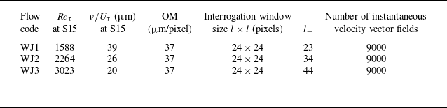
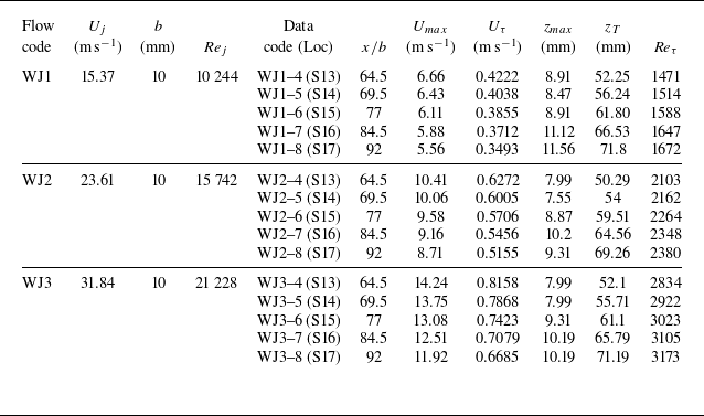
is measured using the oil film interferometry technique as described in detail in Gupta et al. (Reference Gupta, Choudhary, Singh, Prabhakaran and Dixit2020). Salient parameters of the present PIV measurements are summarized in table 1 whereas the flow parameters derived from the PIV data are listed in table 2.
Figure originally from Choudhary et al. (Reference Choudhary, Gupta, Bhatt, Prabhakaran, Singh, Karipot and Dixit2024), i.e. Part 1 and reproduced here with permission. Schematic of the experimental wall jet facility at the Fluid Dynamics Laboratory, IITM, Pune. (a) Three-dimensional (3-D) view of the four-camera arrangement along with the complete long FOV. The PIV measurement plane coincides with the centreline of the test surface. (b) The 2-D side view of the facility. Self-similar region of mean flow development extends from streamwise locations S10 (
 $x/b=49.5$
) to S19 (
 $x/b=107$
); nozzle height
 $b=10$
mm and the streamwise distance
 $x$
is measured from the tip of the upper nozzle lip. The long-FOV PIV domain covers stations S13 through S17. Nomenclature of streamwise measurement stations can be found in Gupta et al. (Reference Gupta, Choudhary, Singh, Prabhakaran and Dixit2020).

Table originally from Choudhary et al. (Reference Choudhary, Gupta, Bhatt, Prabhakaran, Singh, Karipot and Dixit2024), i.e. Part 1 and reproduced here with permission. The PIV measurement parameters for the present experiments. Values of the friction Reynolds number
 ${Re_{\tau }}:={U_{\tau }} z_T/\nu$
and the viscous (wall) length scale
 $\nu /{U_{\tau }}$
are given at location S15 which approximately marks the streamwise centre of the long FOV;
 $\nu$
is the fluid kinematic viscosity and friction velocity,
 $U_{\tau }$
is given by
 ${U_{\tau }}:=\sqrt {\tau _w/\rho }$
wherein
 $\tau _w$
is the wall shear stress and
 $\rho$
is the fluid density. Here OM is optical magnification indicating distance in the measurement plane corresponding to one pixel on the camera sensor. Here
 $l_+=l$
(in pixels)
 $\times$
OM
 $/(\nu /{U_{\tau }})$
denotes the spatial resolution of the PIV measurements in viscous units. Velocity vector fields are obtained in
 $05$
bursts of
 $1800$
frames (one frame has two images taken
 $\textrm {d}t$
apart) obtained simultaneously for all four cameras at
 $6$
Hz; the number
 $1800$
(with four cameras) is dictated by the RAM (128 GB) of the PIV workstation.

Part of this table originally from Choudhary et al. (Reference Choudhary, Gupta, Bhatt, Prabhakaran, Singh, Karipot and Dixit2024), i.e. Part 1 and reproduced here with permission. Flow parameters from the present PIV measurements. Three nozzle Reynolds numbers are indicated by WJ1, WJ2 and WJ3. Here
 $ \textit{Re}_{\tau }$
values are based on the
 $z_{T}$
values from the PIV mean velocity profiles.

(a) Schematic of the mean velocity profile of the wall jet flow. Two reference locations are indicated, one in the inner region (
 ${z^{r}_{+}} \approx 70$
) and the other in the outer region (
 ${z^{r}_{+}} \approx 0.7{Re_{\tau }}$
). The binning of PIV fields is carried out based on the dominant Fourier wavelengths present at these two reference locations. (b) Schematic profile of Reynolds shear stress along with the mean velocity profile. The region between the dashed horizontal lines below the velocity maximum is the region of counter-gradient momentum diffusion.

1.2. Outline of the present paper
The present paper contains three main analyses of the experimental data. Section 2 investigates the large-scale, quasiperiodic coherent patterns in streamwise velocity fluctuation
 $u(x,z)$
fields;
 $x$
and
 $z$
are the streamwise and wall-normal coordinates. First, a modal binning of PIV fields is performed based on the dominant Fourier wavelengths present at a reference height in
 $u(x,z)$
fields. Two reference heights are chosen as shown in figure 3(a). The outer reference height corresponds to the outer energy site whereas the inner reference height is located in the mesolayer. Large-scale coherent patterns observed in individual
 $u(x,z)$
fields are then discussed. This is followed by the presentation of ensemble-averaged modal coherent patterns obtained from the two-point correlations
 $R_{uu}(\Delta x,z)$
of
 $u(x,z)$
fields. There have been studies in the wall-jet literature investigating some aspects of such patterns (Banyassady & Piomelli Reference Banyassady and Piomelli2014; Gnanamanickam et al. Reference Gnanamanickam, Bhatt, Artham and Zhang2019). However, they do not share the privilege of long-FOV experimental 2-D PIV data and measurements over a range of Reynolds numbers, making it impossible to study the long and most-energetic structural modes and their Reynolds number dependence. Also, our long-FOV measurements enable direct estimation of spatial spectra without resorting to Taylor’s hypothesis of frozen turbulence. While the two-point correlations enable deduction of coherent patterns, they do not provide clues about the underlying vortical structures. Section 3, therefore, presents an inquiry into the large-scale vortical structures. These have not been studied so far in the literature on wall jets. The present study attempts to fill this gap with a comprehensive investigation of not only the instantaneous and averaged structures but also the modal structures and their Reynolds number dependence. First, the vortex identification criterion adopted in the present work is discussed, followed by the identification of vortex packets in the Galilean-transformed instantaneous velocity vector fields. Next, the total and modal conditionally averaged fields of fluctuating velocity unit vectors are presented using the linear stochastic estimation (LSE) technique. Herein, two novel methodologies are adopted. First, the swirl strengths of the basic LSE fields are plotted in the background to aid an objective identification of vortices in the LSE fields. Second, the quadrant events are marked in the inner region (below velocity maximum) of the LSE fields to understand the implications of the modal structures towards generating momentum flux in the inner region. The LSE with these two novel methodologies clearly brings out the distinct vortical structures of submode 1 and submode 2 and their roles towards mometum flux generation in the inner region. Section 4 presents regular quadrant analysis using streamwise and wall-normal (
 $u$
and
 $w$
) fluctuating velocity components. These are usual quadrants plotted at various heights from the wall and at different Reynolds numbers. The quadrants seen in LSE are biased towards strong values of LSE condition whereas quadrants in § 4 are unbiased. We first discuss in § 4 how a planar local eddy always transports momentum down the gradient of mean velocity irrespective of its sense of rotation. Therefore, within the planar eddy-framework, the counter-gradient momentum diffusion in wall jets (figure 3
b), occurring just below the mean velocity maximum should be attributed to the non-local eddies. Using this insight, the counter-gradient region is analysed in detail by objectively (yet empirically) segregating fields that have quadrant contributions by the local and non-local eddies dominating in that region. The key highlight from the quadrant analysis is that the counter-gradient region is a result of the intrusion of non-local eddies of the outer jet mode into the inner region and their interaction with the local inner jet mode eddies. This provides the first-ever confirmation of the ‘long arm effect’ of the jet that was envisaged by Professor Narasimha decades ago (Narasimha Reference Narasimha1990) but never confirmed to date. Section 5 summarizes the conclusions of this work.
2. Large-scale coherent patterns in
 $u$
fluctuation fields

2.1. Binning of PIV fields based on the dominant fourier wavelengths
Long-FOV PIV has been a promising approach to study the large-scale coherent patterns in turbulent flows (de Silva et al. Reference de Silva, Kevin, Baidya, Hutchins and Marusic2018). Within a PIV field, the large-scale coherence can usually be discerned from the dominant periodicity present in a particular direction. For example, Hutchins et al. (Reference Hutchins, Ganapathisubramani and Marusic2004, Reference Hutchins, Ganapathisubramani and Marusic2005) analyse the very large scale features in TBLs using spanwise Fourier wavelengths. They present stereo PIV measurements in a plane inclined at
 $45^{\textrm {o}}$
to the
 $y$
–
 $z$
plane. It is shown that simple statistical averaging across all fields tends to mask the spanwise periodicities evident in the individual PIV fields. To bring out these patterns clearly, a method of ‘binning’ the PIV fields is employed based on the dominant Fourier wavelengths obtained from the premultiplied spectra of fluctuating velocity fields. Meaningful averages, such as two-point correlations, are then constructed from these binned PIV fields. More recently, de Silva et al. (Reference de Silva, Chandran, Baidya, Hutchins and Marusic2020) use a similar approach to investigate the large scale coherent patterns in TBLs.
For wall jets, two-point correlations from ‘binned’ velocity fields have not been studied so far and our long-FOV PIV data present an opportunity to explore them. However, broadband two-point correlations in wall jets have been reported before. For example, Banyassady & Piomelli (Reference Banyassady and Piomelli2014) present large-eddy simulations of smooth and rough wall jet flow. Two-point correlations at two reference locations
 $z_{+} \approx 30$
and
 $z_{+} \approx 100$
are presented. At
 $z_{+} \approx 30$
, the contour map is seen to be elliptical in shape (with its major axis tilted at an angle to the streamwise direction) whereas at
 $z_{+} \approx 100$
, the contour map closely resembles a boomerang shape which is attributed to the interaction of the wall eddies with the outer jet structure. Gnanamanickam et al. (Reference Gnanamanickam, Bhatt, Artham and Zhang2019) present two-point correlations of velocity fluctuations
 $u$
and
 $w$
and instantaneous Reynolds shear stress
 $-uw$
from their PIV fields at a single Reynolds number. They compute inclination angle using the correlation contour levels based on the method described in Christensen & Wu (Reference Christensen and Wu2005).
Part 1 of our study reports direct spatial spectral analysis of the long-FOV PIV fields. It is proposed therein that the streamwise motions with wavelengths
 ${{\lambda _{x}}/{z_{T}}}\geqslant 1$
constitute motions that purely belong to the jet mode of the structure of wall jet. Also, it is proposed that the empirical spectral cutoff
 ${{\lambda _{x}}/{z_{T}}}=1$
separates the long wavelength jet mode motions from the mix of shorter wavelength jet and wall mode motions. Further, the study reveals that the jet mode contains two dominant submodes (submode 1 having
 ${\lambda _{x}}\approx 5{z_{T}}$
and submode 2 having
 ${\lambda _{x}}\approx 2.5{z_{T}}$
). These submodes are observed to reside above as well as below the mean velocity maximum. Therefore, it is meaningful to ‘bin’ our long-FOV PIV fields corresponding to the jet mode motions
 ${{\lambda _{x}}/{z_{T}}}\geqslant 1$
with specific focus on submode 1 and submode 2. Further, in a given field, it is required to choose a wall-normal location, referred to as the reference location (denoted by the superscript
 $r$
), where the dominant Fourier wavelength is to be checked for ‘binning’. Part 1 of our study suggests two such locations. In the outer region of flow, i.e. above the mean velocity maximum, the location
 ${z^{r}_{+}} \approx 0.7{Re_{\tau }}$
(
 $\eta ^r$
fixed at
 $\approx 0.7$
) is a justified choice since it is energetically relevant due to the outer energy site of
 $u$
fluctuations (see Part 1). In the inner region, i.e. below the mean velocity maximum,
 ${z^{r}_{+}} \approx 70$
is a reasonable choice (with the available wall-normal resolution of the PIV fields) since it is sufficiently close to the wall while remaining in the mesolayer for all three Reynolds numbers studied here. We therefore use these two locations (figure 3) as the reference locations for ‘binning’ the PIV fields for all three Reynolds numbers. It may be noted that the values of friction velocity
 $U_{\tau }$
and the outer length scale
 $z_{T}$
vary across the long FOV. Therefore, the reference locations
 ${z^{r}_{+}} \approx 0.7{Re_{\tau }}$
and
 ${z^{r}_{+}} \approx 70$
correspond to the streamwise station S15 which is located at the approximate centre of the long FOV. Appendix A gives details of the procedure used to compute the dominant Fourier wavelengths in the long-FOV
 $u(x,z)$
fields.
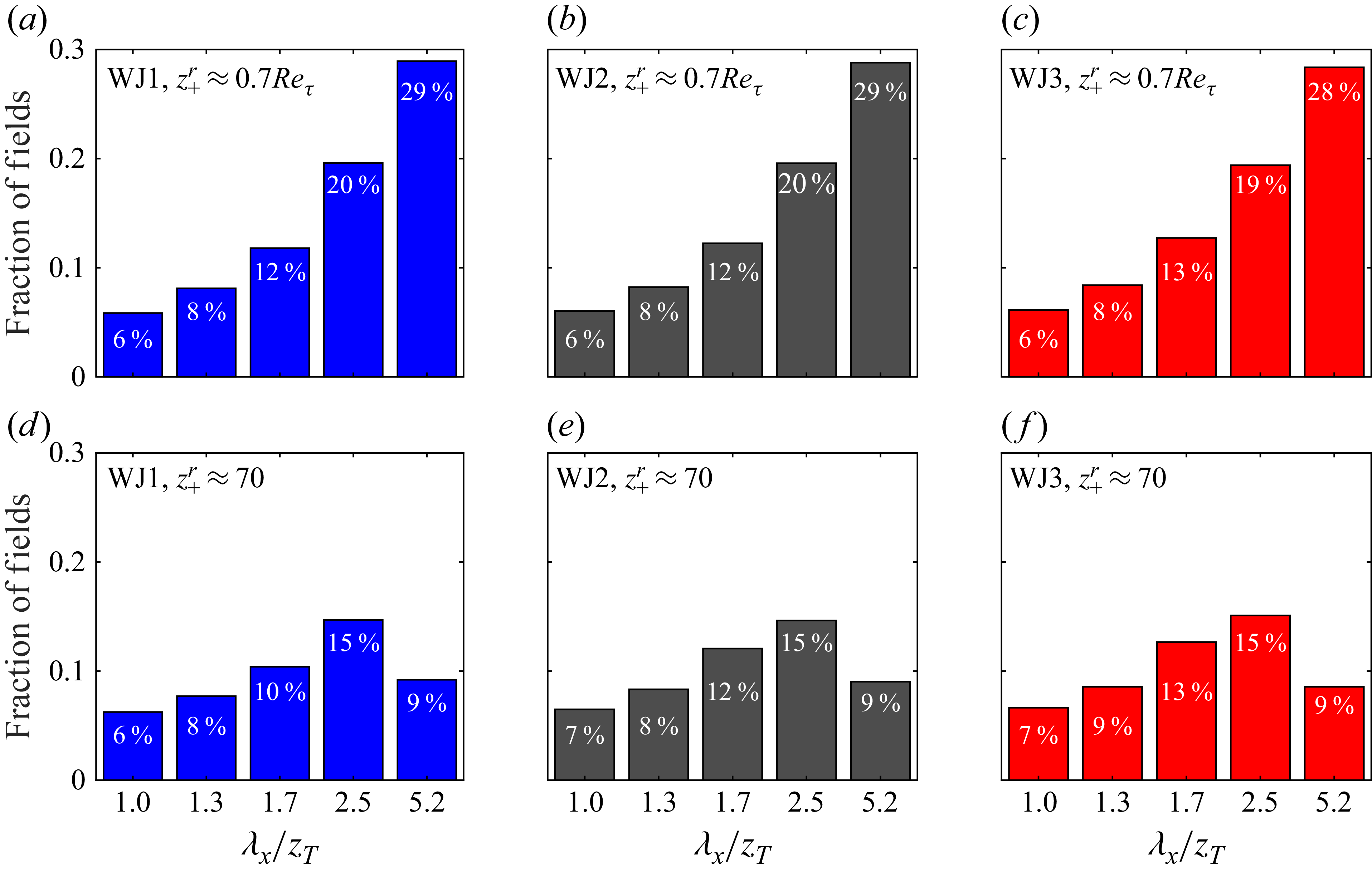
Distribution of the fraction of the total (9000) streamwise velocity fluctuation
 $u(x,z)$
fields exhibiting dominant Fourier wavelengths
 ${\lambda _{x}}\approx 5{z_{T}}$
,
 $2.5{z_{T}}$
,
 $1.7{z_{T}}$
,
 $1.3{z_{T}}$
and
 $z_{T}$
. Panels (a)–(c) show the distributions when binned at the reference location
 ${z^{r}_{+}} \approx 0.7{Re_{\tau }}$
in the outer region, whereas panels (d)–(f) show them when binned at
 ${z^{r}_{+}} \approx 70$
in the inner region. Panels (a) and (d) are for flow WJ1 (blue), (b) and (e) for WJ2 (black), (c) and (f) for WJ3 (red).

Figure 4(a–c) present the fraction of fluctuation PIV velocity fields ‘binned’ according to the first five dominant Fourier modes found at the outer site reference location
 ${z^{r}_{+}} \approx 0.7{Re_{\tau }}$
in the outer region (figure 3). These dominant Fourier modes belong to the outer jet mode motions since the wavelengths are
 $5{z_{T}}$
,
 $2.5{z_{T}}$
,
 $1.7{z_{T}}$
,
 $1.3{z_{T}}$
and
 $z_{T}$
, respectively, i.e.
 ${{\lambda _{x}}/{z_{T}}}\geqslant 1$
. Data for three Reynolds numbers – WJ1(blue), WJ2(grey) and WJ3 (red) are shown. Note that, almost three quarters of the fields (
 $\sim 75\,\%$
) have dominant outer jet mode Fourier wavelengths
 ${{\lambda _{x}}/{z_{T}}}\geqslant 1$
. This is consistent with a large contribution (
 $\sim 79\,\%$
) to the broadband
 $\overline {u^{2}}$
coming from these motions at the outer energy site of
 $u$
fluctuations (figure 10 in Part 1). Further, almost half of the fields (
 $\sim \kern-1pt 47\,\%{-}49\,\%$
) have
 $5{z_{T}}$
and
 $2.5{z_{T}}$
as the dominant Fourier wavelengths suggesting that they are major contributors to the outer energy site. The fraction of fields belonging to the
 ${\lambda _{x}}\approx 5{z_{T}}$
bin is the highest and progressively reduces with the reduction in wavelength. Interestingly, the bar graphs of figure 4(a–c) exhibit no strong dependence on Reynolds numbers suggesting Reynolds number similarity of the outer jet mode in terms of even the fractional occurrences.
Figure 4(d–f) show similar results for the reference location
 ${z^{r}_{+}} \approx 70$
in the inner region (mesolayer). Although this location is quite close to the wall, the dominant inner jet mode Fourier wavelengths
 ${{\lambda _{x}}/{z_{T}}}\geqslant 1$
occur in almost
 $50\,\%$
of the fields which is quite remarkable. Further, these wavelengths progressively occur in
 $48\,\%$
,
 $51\,\%$
and
 $53\,\%$
of the fields in flows WJ1, WJ2 and WJ3, respectively. This suggests a weak, yet discernible, Reynolds number dependence, most of which appears to come from the lowest three dominant wavelengths viz.
 $1.7{z_{T}}$
,
 $1.3{z_{T}}$
and
 $z_{T}$
; the fractions
 $9\,\%$
and
 $15\,\%$
corresponding to the inner jet submodes 1 and 2 (wavelengths
 $5{z_{T}}$
and
 $2.5{z_{T}}$
), on the other hand, exhibit Reynolds number similarity. These observations are in line with our previous findings where the wall and jet regions of the mean velocity description (Gupta et al. Reference Gupta, Choudhary, Singh, Prabhakaran and Dixit2020) and turbulence structure (Part 1) are shown to overlap to yield a non-inertial mesolayer that retains residual dependence on Reynolds number. One may therefore speculate a plausible ‘structural mode mixing’ of wall and jet modes extending from shorter wavelengths up to the wavelength
 ${\lambda _{x}}\approx 1.7{z_{T}}$
; however, study of this aspect would be an elaborate exercise in itself and therefore out of the scope of the present paper. Finally, submode 2 emerges as the most dominant wavelength at this height and the fraction of fields reduces on its either side.
In what follows, we shall specifically focus on the Reynolds-number-independent dominant submodes 1 and 2 of the jet mode structure and investigate their instantaneous and averaged features in some detail using ‘binned’ fields. Also, we shall be predominantly concerned with the fields of velocity fluctuation
 $u(x,z)$
(or
 $w(x,z)$
) extracted from the instantaneous velocity fields
 ${\tilde {u}}(x,z)$
(or
 ${\tilde {w}}(x,z)$
) by subtracting the mean velocity field
 ${U}(x,z)$
(or
 ${W}(x,z)$
) from them.
2.2. Coherent patterns in individual
$u$
fluctuation fields

Figures 5(a) and 5(d), respectively, show sample fields of
 $u_+ (x,z)$
from the bins of two dominant submode wavelengths
 $5{z_{T}}$
(submode 1) and
 $2.5{z_{T}}$
(submode 2). The reference height is
 ${z^{r}_{+}} \approx 0.7{Re_{\tau }}$
indicated by a black dash–dotted line. Black dashed line marks the height
 $z_{\textit{max}}$
of maximum mean velocity
 $U_{\textit{max}}$
over the complete extent of the FOV in each of the plots. The values of
 $u(x,z)$
are normalized by the friction velocity
 $U_{\tau }$
at the centre of the FOV (
 $x/b \approx 77$
, i.e. location S15). In each of the plots, pronounced large-scale streamwise coherence (a near-periodic pattern) is evident from the positive and negative fluctuation regions seen in red and blue colours, respectively. Such large-scale coherence is expected to contribute a significant fraction of TKE at high Reynolds numbers (Smits, McKeon & Marusic Reference Smits, McKeon and Marusic2011).
(a) A representative field of
 $u_+(x,z)$
from the submode 1 bin (
 ${\lambda _{x}}\approx 5{z_{T}}$
) of flow WJ1. The values of
 $u(x,z)$
are normalized by
 $U_{\tau }$
at S15 location (
 $x/b\approx 77$
). Streamwise distance
 $x$
is normalized by the nozzle height
 $b$
, and wall-normal distance
 $z$
is normalized by the outer length scale
 $z_{T}$
. The dash–dotted line represents the binning reference height
 ${z^{r}_{+}} \approx 0.7 {Re_{\tau }}$
in the outer region at S15 (
 $x/b\approx 77$
) and dashed line shows the variation of the height of mean velocity maximum (
 $z_{\textit{max}}$
) in the streamwise direction. (b) Spatial signal
 $u_+(x/b)$
(jagged red line) from (a) at the reference height of
 ${z^{r}_{+}} \approx 0.7 {Re_{\tau }}$
and its spectrally filtered component retaining only the submode 1 wavelength (smooth curve in blue). (c) Spectrally filtered spatial field of
 $u_+(x,z)$
where each row of the field is filtered to retain only the submode 1 wavelength. (d–e) Similar analysis for a representative field of
 $u_+(x,z)$
from the submode 2 bin (
 ${\lambda _{x}}\approx 2.5{z_{T}}$
) of flow WJ1.

(a) A representative field of
 $u_+(x,z)$
from the submode 1 bin (
 ${\lambda _{x}}\approx 5{z_{T}}$
) of flow WJ1. The values of
 $u(x,z)$
are normalized by
 $U_{\tau }$
at S15 location (
 $x/b\approx 77$
). Streamwise distance
 $x$
is normalized by the nozzle height
 $b$
, and wall-normal distance
 $z$
is normalized by the outer length scale
 $z_{T}$
. The dash–dotted line represents the binning reference height
 ${z^{r}_{+}} \approx 70$
in the inner region (mesolayer) at S15 (
 $x/b\approx 77$
) and dashed line shows the variation of the height of mean velocity maximum (
 $z_{\textit{max}}$
) in the streamwise direction. (b) Spatial signal
 $u_+(x/b)$
(jagged red line) from (a) at the reference height of
 ${z^{r}_{+}} \approx 70$
and its spectrally filtered component retaining only the submode 1 wavelength (smooth curve in blue). (c) Spectrally filtered spatial field of
 $u_+(x,z)$
where each row of the field is filtered to retain only the submode 1 wavelength. (d–e) Similar analysis for a representative field of
 $u_+(x,z)$
from the submode 2 bin (
 ${\lambda _{x}}\approx 2.5{z_{T}}$
) of flow WJ1.

Figures 5(b) and 5(e) show the spatial signals of
 $u_+ (x)$
in red colour, extracted from the reference location – the black dash–dotted line – in figures 5(a) and 5(d), respectively. The blue curves in figures 5(b) and 5(e), respectively, show the bandpass-filtered
 $u_+(x)$
signals allowing only Fourier wavelengths
 $5{z_{T}}$
(submode 1) and
 $2.5{z_{T}}$
(submode 2) and setting all other Fourier coefficients to zero. The bandpass-filtered signals faithfully capture the slow variations of the
 $u_+(x)$
signals as expected. Figures 5(c) and 5(f) show the ‘filtered’ versions of figures 5(a) and 5(d), respectively, with the corresponding bandpass filters passing the submode Fourier wavelengths of
 $5{z_{T}}$
and
 $2.5{z_{T}}$
for all pixel rows in each field. Each filtered field shows that the corresponding submode is present across the entire height of the field, not only in the region above the velocity maxima line but also below it. The large-scale coherence in the submode 1 (
 ${\lambda _{x}}\approx 5{z_{T}}$
) filtered field of figure 5(c) shows a forward leaning pattern below the velocity maximum and near-vertical coherent patchs above it. In submode 2 (
 ${\lambda _{x}}\approx 2.5{z_{T}}$
) filtered field of figure 5(f), on the other hand, the patterns are backward leaning above the velocity maxima line and forward leaning (and with a phase shift) below it. These results are consistent with the spectral maps of
 $u$
shown in Part 1 of this study.
Figure 6(a–f) show similar plots when the reference location for binning the fields is chosen to be in the inner region at
 ${z^{r}_{+}} \approx 70$
(horizontal dash–dotted line), i.e. in the mesolayer overlap region. Figures 5 and 6 illustrate that large-scale coherent patterns are evident in individual
 $u$
fluctuation fields.
2.3. Coherent patterns from two-point correlations of
$u$
fluctuation

Contours of the two-point correlation coefficient
 $R_{uu}(\Delta x, z)$
, computed with the reference points
 $(x^r,z^r)$
located at the height of
 ${z^{r}_{+}} \approx 0.7{Re_{\tau }}$
in the outer region (dash–dotted horizontal line), from the binned and total
 $u(x,z)$
fields. The contours are plotted in the
 $x$
–
 $z$
plane with the streamwise distance
 $\Delta x$
from the reference point and wall-normal distance
 $z$
from the wall made dimensionless using
 $z_{T}$
at S15. Panels (a)–(e) show results for flow WJ1 and panels (f)–(j) show the corresponding results for flow WJ3. Horizontal dashed line shows the height of velocity maximum (
 $z_{\textit{max}}$
) at S15 (
 $x/b\approx 77$
). White line passing through the blue dots shows inclination of the outer-layer, backward-leaning pattern. Information on the bin, its corresponding wavelength, fraction of the fields in that bin and the inclination angle are given above each panel.

Contours of two-point correlation
 $R_{uu}(\Delta x,z)$
of the streamwise velocity fluctuation fields
 $u(x,z)$
are routinely plotted to identify the statistically robust coherent patterns in turbulent flows. These are typically dominated by the large-scale coherent motions in the flow whose stronger correlations survive through the process of statistical averaging. For wall jets,
 $R_{uu}$
contours have been plotted before (Gnanamanickam et al. Reference Gnanamanickam, Bhatt, Artham and Zhang2019) albeit with a shorter FOV. Here, we have the advantage of a long FOV that enables observing true sizes of the statistically averaged patterns without resorting to Taylor’s hypothesis.
Computation of
 $R_{uu}(\Delta x,z)$
is carried out as follows. In a field of
 $u(x,z)$
, a reference location
 $(x^r,z^r)$
is selected at the reference height
 $z^r$
. Since any
 $x$
can be written as
 $x^r + \Delta x$
(and similarly for
 $z$
),
 $u(x,z):=u(x^r+\Delta x,z^r+\Delta z)$
. One then obtains the field of the product
 $u(x^r,z^r)u(x^r+\Delta x,z^r+\Delta z)$
and then ensemble average (denoted by
 $\langle . \rangle$
) a number of such fields to obtain the field of
 $\langle u(x^r,z^r)u(x^r+\Delta x,z^r+\Delta z) \rangle$
. The root mean squared (r.m.s.) values
 $\sqrt {\langle u^{2}(x^r,z^r) \rangle }$
and
 $\sqrt {\langle u^{2}(x^r+\Delta x,z^r+\Delta z)\rangle }$
are also obtained from the same number of fields. The field of the correlation coefficient
 $R_{uu}(x^r,z^r, \Delta x,\Delta z)$
centred around
 $(x^r,z^r)$
is computed as
 \begin{align} R_{uu}(x^r,z^r,\Delta x,\Delta z):=\frac {\displaystyle \langle {u(x^r,z^r)} {u(x^r+\Delta x,z^r+\Delta z)}\rangle }{\displaystyle \sqrt {\langle u^{2}(x^r,z^r)\rangle } \sqrt {\langle u^{2}(x^r+\Delta x,z^r+\Delta z)\rangle }}. \end{align}
To compute smoother contours of
 $R_{uu}$
, further spatial averaging in
 $x$
direction (denoted by
 $\lbrace . \rbrace$
) is performed at height
 $z^r$
(Volino, Schultz & Flack Reference Volino, Schultz and Flack2009). That is, the fields of
 $R_{uu}(x^r,z^r, \Delta x,\Delta z)$
are averaged over all values of
 $x^r$
while holding
 $z^r$
fixed. This involves, before averaging, shifting the contours for each reference point horizontally, so that all reference points are on top of each other; this effectively sets
 $x^r=0$
for the reference point in the averaged contours. The resulting smoothed contours are given by
 \begin{align} R_{uu}(z^r,\Delta x,\Delta z):=\lbrace R_{uu}(x^r,z^r,\Delta x,\Delta z)\rbrace . \end{align}
Since
 $z^r$
is a constant for a given reference row and
 $z:=z^r + \Delta z$
as noted before,
 $R_{uu}(z^r,\Delta x,\Delta z)$
may be simply rewritten as
 $R_{uu}(\Delta x, z)$
.
In our data, the fields of
 $R_{uu}(\Delta x, z)$
can be computed using the binned velocity fields mentioned before. This would enable visualizing coherent patterns corresponding to different submodes. Specifically, we would be interested in fields from (i) only submode 1 bin (
 ${\lambda _{x}}\approx 5{z_{T}}$
), (ii) only submode 2 bin (
 ${\lambda _{x}}\approx 2.5{z_{T}}$
), (iii) submode 1 and submode 2 bins clubbed together, (iv) the remaining bins other than submode 1 and submode 2 bins and (v) all bins clubbed together. It is re-emphasized that the fields have been separately binned for two reference rows namely
 ${z^{r}_{+}} \approx 0.7{Re_{\tau }}$
and
 ${z^{r}_{+}} \approx 70$
and need to be used appropriately while constructing the respective
 $R_{uu}(\Delta x, z)$
fields.
Figure 7 illustrates the contours (levels in steps of
 $0.1$
) of
 $R_{uu}(\Delta x, z)$
for submode 1 fields (figure 7
a), submode 2 fields (figure 7
b), submode 1 and submode 2 fields taken together (figure 7
c), remaining fields other than submode 1 and submode 2 (figure 7
d) and all fields (figure 7
e) for the flow WJ1; similar results for flow WJ3 are in figure 7(f–j). The reference row is located at
 ${z^{r}_{+}} \approx 0.7{Re_{\tau }}$
. Note that,
 $\Delta x$
and
 $z$
are both normalized by the outer length scale
 $z_T$
at the centre of the original FOV (S15 location, i.e.
 $x/b=77$
).
Figure 7(a) demonstrates the near-periodic patterns of length scale
 $\approx 5{z_{T}}$
indicating submode 1 periodicity. Note that, the contour values are asymmetric with the maximum value being unity and the minimum approximately
 $-0.32$
. Therefore, the contour colorbar range of
 $[-0.32,0.32]$
is used so that the patches of negative correlation are clearly visible (Banyassady & Piomelli Reference Banyassady and Piomelli2014; Gnanamanickam et al. Reference Gnanamanickam, Bhatt, Artham and Zhang2019; de Silva et al. Reference de Silva, Chandran, Baidya, Hutchins and Marusic2020). The contours indicate a backward-leaning pattern in the outer region of wall jet flow (Gnanamanickam et al. Reference Gnanamanickam, Bhatt, Artham and Zhang2019). As the velocity maximum (dashed line) is approached from the outer flow, this pattern appears stretched in the streamwise direction possibly due to high velocity in that region. The inclination of this backward-leaning pattern of submode 1 is
 $\beta _{o1}\approx -14^{\circ }$
which is the angle of the white line in figure 7(a); negative sign of
 $\beta _{o1}$
indicates a backward-leaning pattern. This line is a least-squares linear fit to the points marked on the contour levels (
 $0.9$
through
 $0.3$
in steps of
 $0.1$
) with each contour having two points (one with
 $\Delta x \gt 0$
and the other with
 $\Delta x \lt 0$
) that are farthest from the reference location
 $(\Delta x/{z_{T}}=0, \eta =0.7)$
(Christensen & Wu Reference Christensen and Wu2005).
Figure 7(b) shows the quasiperiodic patterns of length scale
 $\approx 2.5{z_{T}}$
which is the submode 2 wavelength. It may be noted that inclination here is somewhat steeper (
 $\beta _{o2}\approx -17^{\circ }$
) than the submode 1 pattern (
 $\beta _{o1}\approx -14^{\circ }$
). Figure 7(c) shows the contours obtained by analysing fields from submode 1 and submode 2 combined together. While the overall features, including the inclination
 $\beta _{o12}\approx -15^{\circ }$
, show dominance of submode 1, the strong negative correlations of submode 1 from figure 7(a) have weakened whereas those of submode 2 from figure 7(b) have completely disappeared due to mixing of modes. Figure 7(d) shows the contours after analysis of fields except submode 1 and submode 2 fields. It is seen that the regions of high correlation are shrunk to a more compact area whereas the regions of lower correlation have expanded. The inclination is
 $\beta _{or}\approx -14^{\circ }$
for these remaining fields. Finally, when all fields are processed without binning, the resulting contours are shown in figure 7(e). The inclination in the outer region is
 $\beta _{o}\approx -14^{\circ }$
on the average and is somewhat lesser than the angle
 $\beta _{j}\approx -18^{\circ }$
reported by Gnanamanickam et al. (Reference Gnanamanickam, Bhatt, Artham and Zhang2019). This difference may be heuristically understood from the differences in lateral boundary conditions between these studies. Our flow is not confined in the lateral (spanwise) direction by sidewalls and therefore freely expands in that direction as it proceeds downstream. In the case of Gnanamanickam et al. (Reference Gnanamanickam, Bhatt, Artham and Zhang2019), the apparatus sidewalls confine the flow laterally and this possibly makes the inclination steeper due to mass conservation. In addition, reference row is located at
 ${z^{r}_{+}} \approx 0.7{Re_{\tau }}$
in our case whereas it is at
 ${z^{r}_{+}} \approx 0.6{Re_{\tau }}$
in the case of Gnanamanickam et al. (Reference Gnanamanickam, Bhatt, Artham and Zhang2019). This could also be contributing to the difference between the inclinations in the outer region from these two studies.
Figure 7(f–j) show the corresponding results for flow WJ3. By comparing the plots for WJ1 and WJ3, overall features of the correlation contours are nearly identical except for a subtle indication that the the correlation extends deeper below the velocity maximum line with increasing Reynolds number. However, this observation requires further confirmation from data at higher Reynolds numbers from the future studies.
Contours of the two-point correlation coefficient
 $R_{uu}(\Delta x, z)$
, computed with the reference points
 $(x^r,z^r)$
located at the height of
 ${z^{r}_{+}} \approx 70$
in the inner region mesolayer (dash–dotted horizontal line), from the binned and total
 $u(x,z)$
fields. The contours are plotted in the
 $x$
–
 $z$
plane with the streamwise distance
 $\Delta x$
from the reference point and wall-normal distance
 $z$
from the wall made dimensionless using
 $z_{T}$
at S15. Panels (a)–(e) show results for flow WJ1 and panels (f)–(j) show the corresponding results for flow WJ3. Horizontal dashed line shows the height of velocity maximum (
 $z_{\textit{max}}$
) at S15 (
 $x/b\approx 77$
). White line passing through the blue dots shows inclination of the inner-layer, forward-leaning pattern. Information on the bin, its corresponding wavelength, fraction of the fields in that bin and the inclination angle are given above each panel.

Figure 8 presents results for flows WJ1 and WJ3 similar to figure 7 but with the reference row now located at
 ${z^{r}_{+}} \approx 70$
, i.e. in the mesolayer. Again the contour colorbar range
 $[-0.32,0.32]$
is used for clear visualization of positive and negative correlation regions. For flow WJ1, figures 8(a) and 8(b), respectively, show correlation patterns of wavelengths
 $\approx 5{z_{T}}$
and
 $\approx 2.5{z_{T}}$
corresponding to submodes 1 and 2. In both submodes, the inner pattern is forward-leaning similar to that in TBLs (Christensen & Wu Reference Christensen and Wu2005). The inclination angles of these modal patterns are
 $\beta _{i1}\approx 6^{\circ }$
(figure 8
a) and
 $\beta _{i2}\approx 9^{\circ }$
(figure 8
b). For submodes 1 and 2 taken together, the inclination is
 $\beta _{i12}\approx 7^{\circ }$
(figure 8
c). The remaining fields except for submodes 1 and 2 bins constitute almost
 $76\,\%$
of the total number of fields and these yield the inclination angle of
 $\beta _{ir}\approx 9^{\circ }$
(figure 8
d). Finally, for the complete set of fields without any binning, the inclination is
 $\beta _{i}\approx 8^{\circ }$
(figure 8
e). In TBLs, the inclination angle is known to be
 $\approx 12^{\circ }$
on the average (Christensen & Wu Reference Christensen and Wu2005) which is larger than
 $\beta _{i}\approx 8^{\circ }$
seen in our wall jet flow. Further, it is noted that the extent of correlation in each plot extends beyond velocity maximum (dashed horizontal line), especially so for submode 1, indicating that the outer flow (above velocity maximum) bears a strong structural link to the inner flow. The boomerang shaped pattern of the overall correlation (figures 8
e and 8
j) is evident above the velocity maximum which was noted earlier in the literature as well (Banyassady & Piomelli Reference Banyassady and Piomelli2014). As remarked in the earlier discussion of figure 7, the patterns of submodes 1 and 2 get masked if one considers the full set of fields without modal binning. In fact, the remarkable similarity between figures 8(d) and 8(e) highlights the fact that the overall correlation plot is dominated by the fields other than the submode 1 and submode 2 fields. For flow WJ3, quantitative differences from WJ1 flow in the correlation plots (figures 8
a and 8
f, figures 8
b and 8
g, etc.) may be discerned. The wall-normal and downstream extent of the correlation increases with Reynolds number which is somewhat expected due to Reynolds number dependence of the mesolayer. Inclination angles show a weak but consistent increase in all panels which could be explained by increase of wall-normal correlation at a higher rate (with Reynolds number) than the downstream correlation. The shape of the boomerang also becomes more unsymmetrical (figure 8
c for WJ1 and figure 8
h for WJ3) with the downstream end progressively stretched out with increasing Reynolds number. These findings are consistent with our contention that it is too simplistic to consider the region below velocity maximum akin to a TBL.
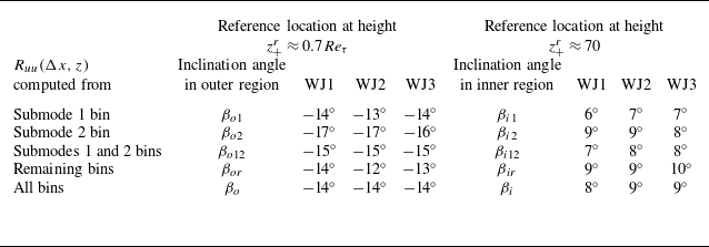
Results of inclination angle for all flows analysed here are given in table 3. A reasonable degree of Reynolds number similarity of the outer-region inclinations (invariance with Reynolds number) and a weak Reynolds number dependence of the inner-region inclinations is suggested by the tabulated values. We also note that the modal two-point correlations here are computed from different subsets of fields binned according to different submodes. Therefore, it is important to ascertain the statistical convergence of the present results. Appendix B discusses this aspect in detail and demonstrates that all the results presented here are indeed statistically well-converged.
Inclination angles from the contours of
 $R_{uu}(\Delta x, z)$
in the present wall jet experiments.

The above analysis highlights strong, large-scale coherent patterns associated with the structural submodes in the outer and inner regions of a wall jet flow and also delineates their periodicities, inclinations and (weak) Reynolds number dependence. The inclinations in the outer and inner regions show only minor variations with the binning strategy (table 3) which is not surprising because the convergence of
 $R_{uu}$
at short distances from the reference point is nearly identical in all the subsets and the near-periodic patterns of submode 1 and submode 2, seen as oscillations in the
 $R_{uu}$
, become evident only away from the reference point. The above analysis, however, does not provide any clues about the coherent vortical structures associated with these submodes. The next section therefore presents an inquiry into these vortical structures.
3. Planar vortical structures in instantaneous and fluctuating velocity fields
3.1. Planar vortex identification using swirl strength criterion
Identifying vortices in a turbulent flow is important to understand the coherent vortical structures present in the flow. Strictly speaking, such vortical structures are highly 3-D and therefore ideally require experimental methods or numerical simulations that can resolve them in three dimensions (Samie et al. Reference Samie, Lavoie and Pollard2021, Reference Samie, Aparece-Scutariu, Lavoie, Shin and Pollard2022). Most experiments, on the other hand, use planar 2-D measurements that effectively display the signatures of these 3-D structures projected into the plane of measurement. It may, however, be noted that despite their limitation of two dimensionality, such studies have significantly enhanced the understanding of coherent vortical structures in wall turbulence (Adrian, Meinhart & Tomkins Reference Adrian, Meinhart and Tomkins2000; Christensen & Wu Reference Christensen and Wu2005; Volino et al. Reference Volino, Schultz and Flack2009). Therefore, here we analyse our planar PIV measurements to discern the planar vortical structures in wall jet flows; henceforth, for the vortices analysed in this work, we shall omit the qualification ‘planar’ for brevity.
In an instantaneous flow field, vortices can usually be visualized as swirling motions around certain points in the flow field, and they become apparent when a certain convection velocity, common to all such vortices, is subtracted from the entire instantaneous flow field. In other words, the idea is to switch to a frame of reference that moves with a vortex or a group of vortices, a Galilean transformation that is allowed by the governing equations. Also, it is known that vortices in wall turbulence can align and travel as vortex packets, with each packet having its own convection velocity (Adrian et al. Reference Adrian, Meinhart and Tomkins2000). However, it is possible that different vortex packets convect at different velocities so that a single convection velocity is, in general, not sufficient to visualize all of them unequivocally. A fundamental approach to identify vortices is to use the rotation part of the velocity gradient tensor. Based on this, different vortex identification criteria have been proposed such as the
 $Q$
criterion (Hunt, Wray & Moin Reference Hunt, Wray and Moin1988),
 $\lambda _2$
criterion (Jeong & Hussain Reference Jeong and Hussain1995),
 $\Delta$
criterion (Chong, Perry & Cantwell Reference Chong, Perry and Cantwell1990),
 $\lambda _{ci}$
criterion (Zhou et al. Reference Zhou, Adrian, Balachandar and Kendall1999), etc. These criteria can be shown to identify vortices in a consensus manner if one uses appropriate thresholds under correct normalizations (Chakraborty, Balachandar & Adrian Reference Chakraborty, Balachandar and Adrian2005). Here, we use the
 $\lambda _{ci}$
, i.e. swirling strength criterion for vortex identification in our 2-D-PIV fields.
Swirl strength (
 $\lambda _{ci}$
) at a point in a flow field is defined as the imaginary part of the complex eigenvalue of the local velocity gradient tensor (Zhou et al. Reference Zhou, Adrian, Balachandar and Kendall1999) and represents the strength of pure rotation at that point. Since our PIV velocity vector fields are 2-D, the velocity gradient tensor is the 2-D matrix. The characteristic equation of this 2-D matrix is a quadratic equation with discriminant denoted by
 $\Delta$
. At points in an instantaneous velocity vector field where
 $\Delta \lt 0$
, the eigenvalues are complex. Therefore, only such points in the velocity vector field where
 $\Delta \lt 0$
are considered for evaluating
 $\lambda _{ci}$
; the value of
 $\lambda _{ci}$
at all other points is set to zero. Mathematically, the swirl strength is given by
 $\lambda _{ci}=\sqrt {\left |\Delta \right |}/2$
and does not have a sign, by definition. However, the sense of rotation can be assigned to
 $\lambda _{ci}$
at a point by multiplying it with the unit vorticity (spanwise) fluctuation
 $\hat {\omega }_y (x,z)$
at the same point (Christensen & Wu Reference Christensen and Wu2005). This signed
 $\lambda _{ci}$
is denoted by
 $\varLambda _{ci}$
and is given by
 $\varLambda _{ci}(x,z):=\lambda _{ci}(x,z)\hat {\omega }_y (x,z)$
wherein
 $\omega _y (x,z)$
is the field of the fluctuating vorticity having clockwise (negative) or anticlockwise (positive) sense. Details of the procedure for computing fields of
 $\varLambda _{ci}(x,z)$
from the fields of
 ${\tilde {u}}(x,z)$
and
 ${\tilde {w}}(x,z)$
is given in Appendix C.1.
It may be noted that
 $\varLambda _{ci}$
has the dimension
 $T^{-1}$
(
 $T$
is the time dimension) and suitable normalization is required to make it dimensionless. Since the gradients in the wall-normal (
 $z$
) direction are significantly stronger than in the streamwise (
 $x$
) direction, an average value of
 $\varLambda _{ci}$
for each row of the FOV could be a reasonable choice. However, since the the positive and negative contributions to the mean value of
 $\varLambda _{ci}$
in each row from all fields are nearly equal, (not shown, see also Wu & Christensen (Reference Wu and Christensen2006)), the mean value of
 $\varLambda _{ci}$
is very small and does not represent the typical value of
 $\varLambda _{ci}$
at that height. Therefore, following Wu & Christensen (Reference Wu and Christensen2006), we use the r.m.s. value of
 $\varLambda _{ci}$
for each row (computed from all 9000 fields) for normalizing
 $\varLambda _{ci}$
as
 \begin{align} \widetilde {\varLambda }_{ci}(x,z):=\dfrac {\varLambda _{ci}(x,z)}{\sqrt {\lbrace \langle \varLambda _{ci}^2(x,z)\rangle \rbrace }}, \end{align}
where
 $\langle . \rangle$
denotes ensemble average across 9000 fields and
 $\lbrace . \rbrace$
denotes the average over the row (in
 $x$
direction), as mentioned before, so that the denominator in (3.1) is a function of
 $z$
alone. In what follows, we shall use
 $\widetilde {\varLambda }_{ci}(x,z)$
for our analysis of instantaneous as well as conditionally averaged fields.
3.2. Vortical structures in instantaneous velocity vector fields
As mentioned before, vortical structures in instantaneous fields of TBLs and channel flows are typically identified using the swirl strength criterion (Adrian Reference Adrian1994; Christensen & Adrian Reference Christensen and Adrian2001; Hambleton, Hutchins & Marusic Reference Hambleton, Hutchins and Marusic2006). However, no prior studies have used this criterion to study the vortical structures in wall jets.
Figure 9(a) shows, in the background, the contour plot of a typical field of streamwise velocity fluctuation
 $u_+(x,z)$
from the bin of submode 1 for WJ1 flow. Overlaid on these contours is the innerscaled, Galilean-transformed instantaneous velocity vector field
 $\boldsymbol{{\tilde {u}}}_{\boldsymbol{G}+}(x,z)$
. For the transformation, a uniform (yet arbitrary) streamwise convection velocity
 $U_{c+} = 0.8U_{\textit{max}}/{U_{\tau }}$
(same as Gnanamanickam et al. Reference Gnanamanickam, Bhatt, Artham and Zhang2019) is subtracted from the inner-scaled, instantaneous velocity vector field
 $\boldsymbol{{\tilde {u}}}_+(x,z)$
. Note that,
 $U_{\textit{max}}$
and
 $U_{\tau }$
correspond to the location S15. Each vector in figure 9(a) is thus made up of two velocity components, namely
 ${\tilde {u}}_+(x,z)-U_{c+}$
and
 ${\tilde {w}}_+(x,z)$
. Mathematically, the Galilean-transformed velocity vector field is given by
 \begin{align} \boldsymbol{{\tilde {u}}}_{\boldsymbol{G}+}(x,z)=\boldsymbol{{\tilde {u}}}_+(x,z)-U_{c+}\hat {\boldsymbol{i}}=\left [{\tilde {u}}_+(x,z)-U_{c+}\right ]\hat {\boldsymbol{i}}+\left [{\tilde {w}}_+(x,z)\right ]\hat {\boldsymbol{k}}, \end{align}
where
 $\hat {\boldsymbol{i}}$
and
 $\hat {\boldsymbol{k}}$
are the unit vectors in
 $x$
and
 $z$
directions, respectively. Note that, for plotting the velocity vectors with correct orientations, it is important to keep the aspect ratio of the plotted panel same as that of the wide FOV of the PIV measurements. Also, for ease of comprehension, streamwise distance
 $(x-x_0)$
is referenced to the start of the FOV (lower left-hand corner) where
 $x_0$
is the distance of the start of PIV FOV from the nozzle exit. Note that,
 $(x-x_0)$
is normalized by
 $z_{T}$
at S15 location. Wall-normal heights are expressed in the outer scaling. A notable correspondence is evident between the contours of
 $u_+(x,z)$
and the Galilean-transformed velocity vector field
 $\boldsymbol{{\tilde {u}}}_{\boldsymbol{G}+}(x,z)$
(figure 9
a). Regions where
 $u_+(x,z)$
contours change sign are found to correspond quite well to the regions where swirling motions appear in the
 $\boldsymbol{{\tilde {u}}}_{\boldsymbol{G}+}(x,z)$
field. A closer look reveals that these swirling motions are mostly anticlockwise and may be reckoned to be a backward-leaning vortex packet where each constituent vortex is advecting (or convecting) downstream at approximately the same velocity equal to
 $0.8U_{\textit{max}}$
. Other choices of convection velocity would expose vortices that could be travelling at those speeds.
(a) Contours of
 $u_+(x,z)$
in the background overlaid with the corresponding Galilean-transformed instantaneous velocity vector field
 $\boldsymbol{{\tilde {u}}}_{\boldsymbol{G}+}(x,z)$
(arrows) after subtracting a constant convection velocity
 $U_{c+}=0.8U_{ {max}+}$
. This field belongs to submode 1 bin of WJ1 flow. Streamwise and wall-normal distances are normalized by the outer length scale
 $z_{T}$
, and
 $U_{\textit{max}}$
,
 $U_{\tau }$
and
 $z_{T}$
correspond to S15 location (
 $x/b \approx 77$
). Distance
 $(x-x_0)$
is measured from the start of the FOV. (b) Same velocity vector field
 $\boldsymbol{{\tilde {u}}}_{\boldsymbol{G}+}(x,z)$
as in (a) with the background changed to contours of normalized, signed swirl strength
 $\widetilde {\varLambda }_{ci}$
(positive anticlockwise). (c) Zoomed view of the region shown by the rectangular box in (b). Upper five circles indicate regions of strong anticlockwise swirls or vortices suggesting an ‘instantaneous’ backward-leaning vortex packet with approximate inclination of
 $30^{\circ }$
. The rightmost circle appears to be somewhat ahead of the packet.

Figure 9(b) shows the contours of strong swirl strength (
 $\widetilde {\varLambda }_{ci}\gt 1$
in red colour,
 $\widetilde {\varLambda }_{ci}\lt -1$
in blue colour and any values in between without colour) plotted in the background of the same
 $\boldsymbol{{\tilde {u}}}_{\boldsymbol{G}+}(x,z)$
field as in figure 9(a). Figure 9(c) shows a zoomed view of the region marked by the rectangle in figure 9(b) where an ‘instantaneous’ vortex packet can be discerned. Figure 9(c) shows that the strong swirling motions (circled) correspond quite well to the patches of intense anticlockwise swirl strength (
 $\widetilde {\varLambda }_{ci}\gt 1$
in red colour) and five of them, except for the rightmost, form a backward-leaning vortex packet. The inclination of this ‘instantaneous’ packet is approximately
 $30^{\circ }$
as marked by the thick dashed line and the packet vertically extends over
 $0.3\leqslant \eta \leqslant 1$
. Further, it may be noted that the rightmost vortex in figure 9(c), although advecting at the same speed, is somewhat ahead of the rest of the packet. For flows WJ2 and WJ3, similar features are observed in instantaneous velocity vector fields and are therefore not shown here for brevity.
3.3. Vortical structures in conditionally averaged fluctuating velocity vector fields
Conditionally averaged fluctuating velocity vector fields provide information on the statistically robust vortical structures in the flow that correspond to certain specific events that are used as the condition for averaging. A common tool to obtain such conditionally averaged fields is the so-called LSE. The LSE is based on the two-point correlation between the velocity fluctuation vector field and the conditioning event. In TBLs and channel flows, swirl strength of instantaneous velocity field and Reynolds shear stress have been used in the literature as conditioning events to unravel vortex organization in wall turbulence (Christensen & Adrian Reference Christensen and Adrian2001; Hambleton et al. Reference Hambleton, Hutchins and Marusic2006; Natrajan & Christensen Reference Natrajan and Christensen2006; Wu & Christensen Reference Wu and Christensen2007; Volino et al. Reference Volino, Schultz and Flack2009). It may be noted that, LSE has been applied to channel flows (Christensen & Adrian Reference Christensen and Adrian2001), which are homogeneous in the streamwise direction but inhomogeneous in the cross-stream (wall-normal) direction. In addition, LSE has been used in TBLs (Volino et al. Reference Volino, Schultz and Flack2009), swirling jets (Gutmark et al. Reference Gutmark, Verfaillie, Bonnet and Grinstein2006) and jet mixing layers (Cole, Glauser & Guezennec Reference Cole, Glauser and Guezennec1992) and these flows are inhomogeneous in the streamwise (due to flow development) as well as cross-stream directions. In the latter cases, the inhomogeneity in the cross-stream direction is, however, much stronger compared with the inhomogeneity in the streamwise direction, i.e.
 $|\partial U/\partial z| \gg |\partial U/ \partial x|$
. Despite these inhomogeneities, the LSE-derived eddies are known to correspond well to the physical eddies in such flows (Adrian Reference Adrian1996). Our wall jets, too, develop in the downstream direction in a manner that
 $|\partial U/\partial z| \gg |\partial U/ \partial x|$
. For instance, from table 2, one may estimate
 $|\partial U/\partial z| \sim {U_{\textit{max}}}/{z_{T}} \approx 214$
 $\textrm {s}^{-1}$
for WJ3 flow at S15. For the same flow,
 $|\partial U/\partial x| \sim \Delta {U_{\textit{max}}}/ \Delta x \approx 8.4$
 $\textrm {s}^{-1}$
estimated over the length of our PIV velocity field. The ratio of these two strain rates is
 $(|\partial U/\partial x|)/(|\partial U/ \partial z|)\approx 0.04$
indicating that the streamwise inhomogeneity is just
 $4\,\%$
of the wall-normal inhomogeneity. In view of this, one may expect the LSE to yield physically meaningful vortical structures in the present wall jets as well.
In the literature on wall jets, statistically robust vortical structures identified through the LSE have not been reported so far. Previous sections indicate that the signed swirl strength
 $\varLambda _{ci}$
from the instantaneous velocity vector fields
 $\boldsymbol{{\tilde {u}}}(x,z)$
correlates well with the vortical structures observed in the Galilean-transformed instantaneous velocity vector fields
 $\boldsymbol{{\tilde {u}}}_{\boldsymbol{G}+}(x,z)$
. Therefore, here we seek to obtain the conditionally averaged fluctuating velocity vector fields
 $\boldsymbol{u_{\textit{LSE}}}(\Delta x,z)$
by performing LSE on the
 $\boldsymbol{u}(x,z)$
fields conditioned on
 $\varLambda _{ci}$
.
In wall jets,
 $\partial U/\partial z \lt 0$
in the region above velocity maximum. Therefore, anticlockwise vorticity is supported by the mean shear, i.e. positive values of
 $\varLambda _{ci}$
represent ‘prograde’ vortices (Wu & Christensen Reference Wu and Christensen2006). Therefore, we focus on LSE fields obtained from the condition
 $\varLambda _{ci}\gt 0$
. This would yield a statistically robust structure of the flow corresponding to prograde vorticity at the reference height in the outer region of the wall jet flow. For the streamwise component of fluctuating velocity, we denote the linear stochastic estimate (Adrian & Moin Reference Adrian and Moin1988; Volino et al. Reference Volino, Schultz and Flack2009), obtained from an ensemble of
 $u(x,z)$
fields, by
 $u_{\textit{LSE}}(z^r,\Delta x,\Delta z)$
and it is given by
 \begin{eqnarray} u_{\textit{LSE}}(z^r,\Delta x,\Delta z)&=&\langle \lbrace u(x^r+\Delta x, z^r+\Delta z) | \varLambda _{ci}(x^r, z^r)\gt 0 \rbrace \rangle \nonumber \\ &=&\frac { \displaystyle \langle \lbrace { \varLambda _{ci}(x^r, z^r)u(x^r+\Delta x, z^r+\Delta z)}\rbrace \rangle } { \displaystyle \langle \lbrace \varLambda _{ci}(x^r, z^r) \varLambda _{ci}(x^r, z^r)\rbrace \rangle } \varLambda _{ci}(1, z^r). \end{eqnarray}
In a given field of
 $u(x,z)$
, the condition
 $\varLambda _{ci}\gt 0$
for prograde swirl strength is checked for all points
 $(x^r,z^r)$
at the reference height
 ${z^{r}_{+}} \approx 0.7{Re_{\tau }}$
and only those points are selected as reference points where this condition is satisfied. The
 $u(x,z)$
field is multiplied all through by each such value of
 $\varLambda _{ci}$
to yield a number of conditional fields of
 $\varLambda _{ci}(x^r, z^r)u(x,z):=\varLambda _{ci}(x^r, z^r)u(x^r+\Delta x, z^r+\Delta z)$
. These fields, generated from a given
 $u(x,z)$
field, are first averaged amongst themselves, by bringing all the reference points on top of each other, to yield a conditionally averaged field corresponding to that
 $u(x,z)$
field. This first level of averaging is denoted by
 $\lbrace .\rbrace$
in the numerator of (3.3). The same procedure is repeated for other
 $u(x,z)$
fields under consideration (all or submode 1 bin or submode 2 bin or all except submode 1 and 2 bins). Finally, all such first-level-averaged
 $\lbrace .\rbrace$
fields are further averaged (second level averaging) as indicated by
 $\langle .\rangle$
in the numerator of (3.3). The denominator in (3.3) is simply the mean squared value of
 $\varLambda _{ci}(x^r, z^r)$
within each field of
 $u(x,z)$
, denoted by
 $\lbrace .\rbrace$
, and then the average, denoted by
 $\langle .\rangle$
, of all such mean squared values over the number of
 $u(x,z)$
fields (all or submode 1 bin or submode 2 bin or all except submode 1 and 2 bins). Note that,
 $\varLambda _{ci}(1, z^r)$
in (3.3) is chosen arbitrarily from the set of all qualifying
 $\varLambda _{ci}(x^r, z^r)$
values since its precise choice does not affect the results (Christensen & Adrian Reference Christensen and Adrian2001) provided the same value is used in all the calculations. The same exercise is repeated for the wall-normal velocity fluctuation component
 $w(x,z)$
fields to obtain
 $w_{\textit{LSE}}(z^r,\Delta x,\Delta z)$
. As mentioned before in § 2.3,
 $z:=z^r+\Delta z$
so that one may simply write the LSE fields as
 $u_{\textit{LSE}}(\Delta x, z)$
and
 $w_{\textit{LSE}}(\Delta x, z)$
. Finally, one constructs the basic LSE fluctuating velocity vector field
 $\boldsymbol{u}_{\textit{LSE}}(\Delta x,z)$
as
 \begin{align} \boldsymbol{u}_{\textit{LSE}}(\Delta x,z):=u_{\textit{LSE}}(\Delta x,z)\hat {\boldsymbol{i}}+w_{\textit{LSE}}(\Delta x,z)\hat {\boldsymbol{k}}. \end{align}
It is recommended to normalize the magnitude of each LSE vector to unity so that only the directions are highlighted in the conditional flow field estimation enabling clear visualization of vortices (Christensen & Adrian Reference Christensen and Adrian2001). This LSE unit vector field
 $\boldsymbol{\hat {u}}_{\textit{LSE}}(\Delta x,z)$
is given by
 \begin{align} \boldsymbol{\hat {u}}_{\textit{LSE}}(\Delta x,z):=\frac {\boldsymbol{u}_{\textit{LSE}}(\Delta x,z)}{\left |\boldsymbol{u}_{\textit{LSE}}(\Delta x,z)\right |}. \end{align}
In what follows, we shall process and plot the LSE unit vector fields
 $\boldsymbol{\hat {u}}_{\textit{LSE}}(\Delta x,z)$
but refer to them as LSE fields, for brevity.
In addition to this LSE procedure that is established in the literature, we employ two novel approaches that enhance the physical interpretations of the LSE fields in our study. First, we compute the signed swirl strength
 $\varLambda _{ci,\textit{LSE}}(\Delta x,z)$
from the basic LSE fluctuating velocity vector fields
 $\boldsymbol{u}_{\textit{LSE}}(\Delta x,z)$
and plot its contours in the background of the LSE fields. This enables identifying swirling (vortical) regions in the LSE fields without ambiguity (anticlockwise rotations have
 $\varLambda _{ci,\textit{LSE}}\gt 0$
and clockwise rotations have
 $\varLambda _{ci,\textit{LSE}}\lt 0$
). Note that, normalization by the r.m.s. value is not required in the case of
 $\varLambda _{ci,\textit{LSE}}$
computed from
 $\boldsymbol{u}_{\textit{LSE}}(\Delta x,z)$
fields; such a normalization, on the other hand, is required for
 $\varLambda _{ci}$
computed from the instantaneous velocity vector fields
 $\boldsymbol{u}(x,z)$
as mentioned before. Details of the procedure for computing fields of
 $\varLambda _{ci, {LSE}}(\Delta x,z)$
from the basic LSE fluctuating velocity vector fields
 $\boldsymbol{u}_{\textit{LSE}}(\Delta x,z)$
is given in Appendix C.2. Secondly, we use LSE field vectors to interpret quadrant events (Wallace, Eckelmann & Brodkey Reference Wallace, Eckelmann and Brodkey1972; Wallace Reference Wallace2016). This is specifically done with the aim to understand quadrant contributions in the counter-gradient momentum diffusion region below velocity maximum when the LSE condition of prograde swirl (
 $\varLambda _{ci}\gt 0$
) is imposed in the outer region; it should be noted that, this approach is different from using quadrant events themselves as the condition for the LSE (Volino et al. Reference Volino, Schultz and Flack2009). It may also be noted that the interpretation of quadrant events from an LSE plot requires some care. First, the quadrant events themselves are always ‘local’ (at a point) in character, the eddy motions contributing to them could be ‘local’ and/or ‘non-local’. Therefore, we shall always refer to the eddy motions as ‘local’ or ‘non-local’. Next, the LSE formalism (3.3) computes the conditionally averaged field where the average is actually a weighted average, the weight being the value of
 $\varLambda _{ci}$
. As a result, the quadrant events seen in an LSE plot are biased towards those fields (centred around the conditioning point) that have stronger
 $\varLambda _{ci}$
. In other words, the quadrant events in an LSE plot would closely represent the reality for those
 $u(x,z)$
fields (centred around the conditioning point) for which the magnitude of
 $\varLambda _{ci}$
is large but might actually miss the reality for fields having smaller magnitude of
 $\varLambda _{ci}$
. This aspect is important for the interpretation of results in § 4 that presents the regular or unbiased quadrant analysis with no such conditions applied.
We now discuss the LSE fields obtained by considering (i) all 9000
 $\boldsymbol{u}(x,z)$
fields, (ii)
 $\boldsymbol{u}(x,z)$
fields only from the submode 1 bin, (iii)
 $\boldsymbol{u}(x,z)$
fields only from the submode 2 bin and (iv) remaining
 $\boldsymbol{u}(x,z)$
fields from all bins except submode 1 and submode 2 bins; binning for (ii) to (iv) is based on the reference row in the outer region at
 ${z^{r}_{+}} \approx 0.7{Re_{\tau }}$
.
3.3.1. LSE using all fields (no binning)
Figure 10(a) shows the LSE field
 $\boldsymbol{\hat {u}}_{\textit{LSE}}(\Delta x,z)$
for flow WJ1 whereas figure 10(b) shows enlarged view of the rectangular region marked in figure 10(a). All
 $9000$
fields of
 $\boldsymbol{u}(x,z)$
are used to perform the LSE according to the procedure mentioned in the preceding section. The horizontal axis is
 $\Delta x$
, the streamwise location of the LSE vectors with respect to the conditioning location; the vertical axis is their distances
 $z$
from the wall. Both
 $\Delta x$
and
 $z$
are normalized by the outer length scale
 $z_{T}$
at S15 (
 $x/b\approx 77$
). Several interesting features are discernible from these plots. At the conditioning location, a prograde (anticlockwise) swirl and
 $\varLambda _{ci,\textit{LSE}}\gt 0$
contours (red background) are observed. This is expected since the LSE is conditioned on
 $\varLambda _{ci}(x)\gt 0$
in the parent instantaneous fields
 $\boldsymbol{{\tilde {u}}}(x,z)$
. A backward-leaning structure is apparent in figure 10(b) in the form of a ridge extending from the velocity maximum (
 $\Delta x/{z_{T}} \approx 1.7$
,
 $\eta \approx 0.15$
) up to the conditioning point (
 $\Delta x/{z_{T}}=0$
,
 $\eta =0.7$
); the streamwise extent of this ridge is
 $\approx 1.7{z_{T}}$
. Aligned with this ridge are the red spots of
 $\varLambda _{ci,\textit{LSE}}\gt 0$
confirming that the ridge indeed corresponds to a backward-leaning vortex packet. It may be noted that earlier LSE studies associate such ridges with vortex packets even when there are apparently no swirling motions along the ridge (Volino et al. Reference Volino, Schultz and Flack2009). The novelty of our approach is the use of
 $\varLambda _{ci,\textit{LSE}}$
to objectively discern the vortices in the packet even when they are not explicitly evident as swirling motions along the ridge. The vortex packets in Galilean-transformed instantaneous velocity vector fields
 $\boldsymbol{{\tilde {u}}}_{\boldsymbol{G}+}(x,z)$
are discussed earlier in § 3.2. Figure 10(b) conclusively demonstrates that such vortex packets are statistically robust structures that are observed even in the averaged fields. Interestingly, a saddle-point topology of LSE vectors is seen embedded in the backward-leaning vortex packet of figure 10(b). The location of this saddle point is
 $(\Delta x/{z_{T}} \approx 1.1, \eta \approx 0.5)$
. Next, figure 10(b) shows clockwise swirling motion and blue spots of
 $\varLambda _{ci,\textit{LSE}}\lt 0$
at and below the velocity maximum in the region
 $\Delta x/{z_{T}} \approx 0.2$
–
 $0.8$
. This clockwise swirling is interesting because it emerges in a statistically robust manner although the LSE is not conditioned on
 $\varLambda _{ci}(x)\lt 0$
in the
 $\boldsymbol{{\tilde {u}}}(x,z)$
fields. Figures 10(c) and 10(d), show that the features discussed above for flow WJ1 are robustly present in flow WJ3 as well.
The LSE field
 $\boldsymbol{\hat {u}}_{\textit{LSE}}(\Delta x,z)$
obtained from all
 $9000$
velocity fluctuation vector fields
 $\boldsymbol{u}(x,z)$
for (a) WJ1 flow and (c) WJ3 flow. Panels (b) and (d) show enlarged views of regions shown by rectangles in (a) and (c), respectively. Background contours are of
 $\varLambda _{ci,\textit{LSE}}$
(red anticlockwise and blue clockwise), the swirl strength of the basic LSE fluctuating velocity vector field
 $\boldsymbol{u}_{\textit{LSE}}(\Delta x,z)$
. Condition for LSE is prograde, anticlockwise swirl strength
 $\varLambda _{ci}\gt 0$
, of the instantaneous velocity vector fields
 $\boldsymbol{{\tilde {u}}}(x,z)$
, at the reference height
 $z^r_{+} \approx 0.7 Re_{\tau }$
(upper dashed line). Thick
 $+$
sign shows the location
 $(\Delta x/{z_{T}}=0,\eta \approx 0.7)$
of the conditioning event. Lower dashed line shows the location of maximum velocity corresponding to S15 location
 $(x/b\approx 77)$
. Below this line in (b) and (d), i.e. in the inner region, the Q1, Q2, Q3 and Q4 quadrant events are marked, respectively, by a rectangle, an ellipse, a square and a circle, as the case may be.

The orientations of
 $\boldsymbol{\hat {u}}_{\textit{LSE}}(\Delta x,z)$
arrows in the LSE field enable identification of different quadrant events that contribute to the Reynolds shear stress
 $(-\overline {uw})$
. Of particular interest is the region immediately below the velocity maximum where the momentum flux is known to be counter-gradient (Narasimha Reference Narasimha1990). For flow WJ1, figure 10(b) shows that the outer, large-scale anticlockwise swirl at the conditioning point (
 $+$
sign) induces a ‘non-local’ flow parallel to the wall below the velocity maximum. However, the large-scale clockwise swirl in the region
 $\Delta x/{z_{T}} \approx 0.2$
–
 $0.8$
, below the velocity maximum, causes this flow to lift up and produce Q1-type events (outward interactions,
 $u_{\textit{LSE}}\gt 0$
and
 $w_{\textit{LSE}}\gt 0$
) between
 $\Delta x/{z_{T}} \approx -0.2$
–
 $0.2$
below the velocity maximum. These Q1 events in the inner region, induced by the ‘non-local’ outer layer swirl, are marked by a rectangle in figure 10(b). Further, the large-scale clockwise swirl in the inner region ‘locally’ induces Q2-type events (ejections,
 $u_{\textit{LSE}}\lt 0$
and
 $w_{\textit{LSE}}\gt 0$
, marked by an ellipse) to its left-hand side and Q4-type events (sweeps,
 $u_{\textit{LSE}}\gt 0$
and
 $w_{\textit{LSE}}\lt 0$
, marked by a circle) to its right-hand side as shown in figure 10(b). Notably, Q3-type events (inward interactions,
 $u_{\textit{LSE}}\lt 0$
and
 $w_{\textit{LSE}}\lt 0$
) are not seen below velocity maximum in these LSE fields that use all 9000 fields of
 $\boldsymbol{u}(x,z)$
without any binning. Figure 10(d) indicates that these quadrant features are discernible in flow WJ3 as well, but are displaced somewhat downstream and wallward than for the flow WJ1. It is known that the regions far away from the conditioning point are fraught with low correlation values making the quantitative estimates less robust (Christensen & Adrian Reference Christensen and Adrian2001). Therefore, we limit the LSE field observations to the region
 $\Delta x/{z_{T}} \approx -0.2$
–
 $1.8$
as seen in figures 10(b) and 10(d).
3.3.2. LSE using fields from submode 1 bin
Figure 11 presents the LSE fields
 $\boldsymbol{\hat {u}}_{\textit{LSE}}(\Delta x,z)$
computed using only the submode 1 fields of
 $\boldsymbol{u}(x,z)$
that account for
 $29\,\%$
of the total fields (figure 4). To facilitate ready comparison, the formats of all panels in figure 11 are kept identical to those of figure 10.
The LSE field
 $\boldsymbol{\hat {u}}_{\textit{LSE}}(\Delta x,z)$
obtained from submode 1 velocity fluctuation vector fields
 $\boldsymbol{u}(x,z)$
for (a) WJ1 flow and (c) WJ3 flow. Panels (b) and (d) show enlarged views of regions shown by rectangles in (a) and (c), respectively. Background contours are of
 $\varLambda _{ci,\textit{LSE}}$
(red anticlockwise and blue clockwise), the swirl strength of the basic LSE fluctuating velocity vector field
 $\boldsymbol{u}_{\textit{LSE}}(\Delta x,z)$
. Condition for LSE is prograde, anticlockwise swirl strength
 $\varLambda _{ci}\gt 0$
, of the instantaneous velocity vector fields
 $\boldsymbol{{\tilde {u}}}(x,z)$
, at the reference height
 $z^r_{+} \approx 0.7 Re_{\tau }$
(upper dashed line). Thick
 $+$
sign shows the location
 $(\Delta x/{z_{T}}=0,\eta \approx 0.7)$
of the conditioning event. Lower dashed line shows the location of maximum velocity corresponding to S15 location
 $(x/b\approx 77)$
. Below this line in (b) and (d), i.e. in the inner region, the Q1, Q2, Q3 and Q4 quadrant events are marked, respectively, by a rectangle, an ellipse, a square and a circle, as the case may be.

Figures 11(b) and 11(d) show a peculiar structure of submode 1 when compared with figures 10(b) and 10(d) where no binning was performed. The anticlockwise swirl at the conditioning point is present as expected, but the clockwise swirl below the velocity maximum location is now quite prominent. This clockwise swirl appears to be sandwiched between the wall and the velocity maximum making its streamwise extent wider. The streamwise extent appears to broaden with Reynolds number,
 $0.3\leqslant \Delta x/{z_{T}} \leqslant 0.7$
for WJ1 flow (figure 11
b) and
 $0.2\leqslant \Delta x/{z_{T}} \leqslant 0.9$
for WJ3 flow (figure 11
d). The wall-normal location of the centre of this swirl also shows Reynolds number dependence. It is located very close to the velocity maximum for WJ1 flow (figure 11
b) but moves closer to the wall for WJ3 flow (figure 11
d). It is re-emphasized that the appearance of this clockwise swirl below the velocity maximum is surprising since the conditioning is performed on anticlockwise swirl strength in the outer part above the velocity maximum. This implies that these two swirls are highly correlated and represent the signature structural building block of submode 1. As such, this clockwise swirl of submode 1 below the velocity maximum appears to be distinct from the clockwise swirls of the wall mode that are expected to organize into the forward-leaning hairpin-type vortex packets in the region very close to the wall. These observations are consistent with the dipole-type distributions noted at long wavelengths in the cospectral maps of Reynolds shear stress reported in figure 14 of Part 1. It is interesting to note that this arrangement of opposite swirls in the outer and near-wall regions closely resembles the so-called double-row vortical structure reported in laminar and transitional wall jets; this point shall be discussed later in some detail.
A third clockwise swirl is apparent above and downstream of the conditioning point in figures 11(b) and 11(d). One may notice that a weaker signature of this third swirl is seen in figure 10 as well, however, its appearance in figure 11 is unmistakeable. The wall-normal position of this swirl in figure 11 appears to be fixed around
 $\eta \approx 0.8$
but its streamwise position shows some Reynolds number dependence,
 $\Delta x/{z_{T}}\approx 0.9$
for WJ1 flow and
 $\Delta x/{z_{T}}\approx 1.3$
for WJ3 flow. Vortex packets of long streamwise extent are absent but instead a tall, near-vertical ridge is seen between
 $\Delta x/{z_{T}}=0.6$
to
 $0.8$
. The contours of
 $\varLambda _{ci,\textit{LSE}}$
in the background reveal that this ridge does not correspond to a vortex packet. Instead, a closer look reveals that the ridge is a result of the saddle-point topology formed by the system of three swirls. The height
 $\eta \approx 0.4$
of the saddle point in figures 11(b) and 11(d) appears to be reasonably invariant with Reynolds number whereas its streamwise location
 $\Delta x/{z_{T}}$
varies weakly with Reynolds number from
 $0.7$
for flow WJ1 to
 $0.8$
for flow WJ3. Interestingly, the height of the saddle point
 $\eta \approx 0.4$
correlates quite well with the height
 $\eta \approx 0.35$
where the velocity fluctuation triple product reaches maximum value in the outer region and the corresponding TKE transport term switches it sign as observed in figures 23 and 26 of Part 1.
Below the velocity maximum, figures 11(b) and 11(d) show that the outer layer anticlockwise swirl induces Q1 events, marked by a rectangle, on the left-hand side of the inner clockwise swirl similar to those in figures 10(b) and 10(d). Interestingly, however, Q3-type events, due to the ‘non-local’ outer layer motions, are now seen below the velocity maximum on the right-hand side of the clockwise swirl, as marked by the square in figures 11(b) and 11(d); these Q3 events are not seen in figures 10(b) and 10(d) where all fields are used for the LSE. The LSE fields of figures 11(b) and 11(d) indicate that the upper clockwise swirl induces, below it, fluctuating velocities from right to left and part of this outer region flow is drawn across the velocity maximum into the inner region by the inner clockwise swirl producing these Q3 events. The Q2 and Q4 events induced by the ‘local’ clockwise swirl near the wall (though less prominent) are also present in the inner region; these are, however, not shown explicitly to avoid clutter.
3.3.3. LSE using fields from submode 2 bin
Figure 12 shows the LSE fields
 $\boldsymbol{\hat {u}}_{\textit{LSE}}(\Delta x,z)$
computed from the submode 2 fields of
 $\boldsymbol{u}(x,z)$
that account for almost
 $20\,\%$
of the total number of fields (figure 4). Figures 12(a) and 12(b) show the results for flow WJ1 whereas figures 12(c) and 12(d) show the results for flow WJ3.
The LSE field
 $\boldsymbol{\hat {u}}_{\textit{LSE}}(\Delta x,z)$
obtained from submode 2 velocity fluctuation vector fields
 $\boldsymbol{u}(x,z)$
for (a) WJ1 flow and (c) WJ3 flow. Panels (b) and (d) show enlarged views of regions shown by rectangles in (a) and (c), respectively. Background contours are of
 $\varLambda _{ci,\textit{LSE}}$
(red anticlockwise and blue clockwise), the swirl strength of the basic LSE fluctuating velocity vector field
 $\boldsymbol{u}_{\textit{LSE}}(\Delta x,z)$
. Condition for LSE is prograde, anticlockwise swirl strength
 $\varLambda _{ci}\gt 0$
, of the instantaneous velocity vector fields
 $\boldsymbol{{\tilde {u}}}(x,z)$
, at the reference height
 $z^r_{+} \approx 0.7 Re_{\tau }$
(upper dashed line). Thick
 $+$
sign shows the location
 $(\Delta x/{z_{T}}=0,\eta \approx 0.7)$
of the conditioning event. Lower dashed line shows the location of maximum velocity corresponding to S15 location
 $(x/b\approx 77)$
. Below this line in (b) and (d), i.e. in the inner region, the Q1, Q2, Q3 and Q4 quadrant events are marked, respectively, by a rectangle, an ellipse, a square and a circle, as the case may be.

Figures 12(b) and 12(d) show clear evidence of a long vortex packet in the outer region of the flow which is confirmed by the contours of positive values of
 $\varLambda _{ci,\textit{LSE}}$
in the background. It is interesting that submode 1 fields do not show any backward leaning vortex packets in the outer region of the flow (figure 11) whereas submode 2 fields do (figure 12). This demonstrates that these submodes are different not only from the viewpoint of their spectral signatures as discussed in Part 1 but also from the structural perspective. A weak saddle-point topology is seen around
 $(\Delta x/z_T \approx 0.7,\eta \approx 0.55)$
and appears to be reasonably invariant with Reynolds number (figures 12
b and 12
d). The region below velocity maximum shows only Q1-type events, induced by the ‘non-local’ outer layer motions, (rectangles in figures 12
b and 12
d) in these submode 2 LSE fields.
3.3.4. LSE using fields from the remaining bins (other than submode 1 and submode 2 bins)
Figure 13 shows the LSE fields
 $\boldsymbol{\hat {u}}_{\textit{LSE}}(\Delta x,z)$
computed from the remaining
 $\boldsymbol{u}(x,z)$
fields, other than those from submode 1 and submode 2 bins. These remaining fields account for almost
 $51\,\%$
of the total number of fields (figure 4). As before, figures 13(a) and 13(b) show the results for flow WJ1 whereas figures 13(c) and 13(d) show the results for flow WJ3.
The LSE field
 $\boldsymbol{\hat {u}}_{\textit{LSE}}(\Delta x,z)$
obtained from the remaining (other than submode 1 and submode 2) velocity fluctuation vector fields
 $\boldsymbol{u}(x,z)$
for (a) WJ1 flow and (c) WJ3 flow. Panels (b) and (d) show enlarged views of regions shown by rectangles in (a) and (c), respectively. Background contours are of
 $\varLambda _{ci,\textit{LSE}}$
(red anticlockwise and blue clockwise), the swirl strength of the basic LSE fluctuating velocity vector field
 $\boldsymbol{u}_{\textit{LSE}}(\Delta x,z)$
. Condition for LSE is prograde, anticlockwise swirl strength
 $\varLambda _{ci}\gt 0$
, of the instantaneous velocity vector fields
 $\boldsymbol{{\tilde {u}}}(x,z)$
, at the reference height
 $z^r_{+} \approx 0.7 Re_{\tau }$
(upper dashed line). Thick
 $+$
sign shows the location
 $(\Delta x/{z_{T}}=0,\eta \approx 0.7)$
of the conditioning event. Lower dashed line shows the location of maximum velocity corresponding to S15 location
 $(x/b\approx 77)$
. Below this line in (b) and (d), i.e. in the inner region, the Q1, Q2, Q3 and Q4 quadrant events are marked, respectively, by a rectangle, an ellipse, a square and a circle, as the case may be.

These plots do not show features as significant as the earlier plots. The anticlockwise swirl at the conditioning point occurs as expected. There appears to be some indication of a clockwise swirl in the inner region which is reminiscent of the double-row vortical structure typical of free jets, but its signature is not consistent across the range of Reynolds numbers. Also, the three-vortex system or long vortex packets are absent in the LSE of these remaining fields. Region below the velocity maximum shows Q1-, Q2- and Q4-type quadrant events in WJ1 flow (figure 13 b) and Q1- and Q4-type quadrant events in WJ2 flow (figure 13 d).
3.3.5. Summary of the vortical structures in LSE fields
The LSE analysis presented above sheds light on two kinds of statistically robust turbulent vortical structures of the jet mode in a wall jet flow, subject to the condition of ‘prograde’ (consistent with the mean shear) swirling at the reference height
 ${z_{+}}\approx 0.7{Re_{\tau }}$
in the outer region. The structure of submode 1 is a system of three swirls (vortices) of which, the first is a anticlockwise swirl located at the conditioning point in the outer region. The second is a clockwise swirl located in the near-wall region below velocity maximum (moving closer to the wall with increasing Reynolds number) and somewhat downstream of the first swirl. This arrangement of staggered, opposite swirls on both sides of the velocity maximum is very similar to the double-row structure seen in plane free jets (Gordeyev & Thomas Reference Gordeyev and Thomas2000, Reference Gordeyev and Thomas2002) as well as transitional plane wall jets (Bajura & Szewczyk Reference Bajura and Szewczyk1970; Bajura & Catalano Reference Bajura and Catalano1975; Gogineni & Shih Reference Gogineni and Shih1997; Gogineni, Visbal & Shih Reference Gogineni, Visbal and Shih1999). Numerical simulations of transitional wall jets show that the lower clockwise swirl is generated as a response to the outer anticlockwise swirl according to Kelvin’s circulation theorem. As such, this inner clockwise swirl is inviscid in character, different from the resident boundary layer vorticity, and occurs even when slip is allowed at the bottom wall (Gogineni et al. Reference Gogineni, Visbal and Shih1999). The clockwise swirl below velocity maximum in our LSE fields is also associated with the jet submode 1 which is inherently an inviscid structural mode. Indeed, the observed jet scaling of the mean velocity profiles extending below the velocity maximum in the study by Gupta et al. (Reference Gupta, Choudhary, Singh, Prabhakaran and Dixit2020), can be attributed to the submode 1 jet structure uncovered here. The third clockwise swirl occurs in the outer region farther downstream of the lower clockwise swirl, and apparently has no counterpart in the literature on free jets and transitional wall jets. The physical reason for this third swirl is unclear at the moment and needs further investigation preferably using tomographic PIV. This system of three swirls produces a saddle-point topology of the velocity field around
 $\eta \approx 0.4$
that correlates very well with the transport of turbulence kinetic energy away from this wall-normal location as seen in Part 1 of this study. The structure of submode 2 is a long, backward-leaning vortex packet in the outer region of the flow and this too, apparently does not have a counterpart in the literature on the free jets and transitional wall jets. It may be noted that the mushroom-type vortical structures noted by Gnanamanickam et al. (Reference Gnanamanickam, Bhatt, Artham and Zhang2019) in the instantaneous velocity fields, have much smaller scales and and they do not appear in a statistically robust manner in the present LSE fields. The LSE of fields from all bins other than the submodes 1 and 2 bins, reveal no particularly interesting statistically robust structural features. As such, the LSE of all fields (without any modal binning) predominantly shows a combination of the structures of submodes 1 and 2. It may be mentioned here that the LSE analysis can be carried out in a variety of ways that could differ from each other in terms of the condition being imposed and the location where it is being imposed (Volino et al. Reference Volino, Schultz and Flack2009); here the criterion of ‘prograde’ swirl in the outer region, which is relevant to the present work, is considered. Exploring different variants of the LSE analysis would be an exercise in itself which is out of the scope of the present paper.
Some clarifications on the analyses of §§ 2.3 and 3.3 are in order. First, while both the analyses are covariance-based and performed on the binned as well as full sets of fluctuating velocity fields, there are some important differences between them. For instance, the two-point correlation analysis of § 2.3 is not a conditional analysis as there is no condition imposed on
 $u(x^r,z^r)$
at the reference point ((2.1) and (2.2)). On the other hand, the LSE analysis of § 3.3 is a conditional analysis where the condition
 $\varLambda _{ci}(x^r,z^r)\gt 0$
is imposed (3.3). Secondly, the value of
 $R_{uu}$
at the reference point
 $(x^r,z^r)$
in plots of § 2.3 is guaranteed to be unity due to autocovariance, but this is not the case for the LSE analysis of § 3.3. Third, the coherent patterns in the plots of § 2.3 are deduced from the fields of (signed) magnitude of
 $R_{uu}$
whereas the vortical patterns in any plot of § 3.3 are deduced from the directions (magnitudes are set to unity) of the corresponding LSE unit vector field
 $\boldsymbol{\hat {u}}_{\textit{LSE}}(\Delta x,z)$
. Thus, the outer-layer backward leaning patterns evident in the
 $R_{uu}$
plots of § 2.3 are more or less identical for all subsets simply due to the near-identical convergence of the spatial autocovariance around the reference point. On the other hand, each submode has a distinct vortical structure as revealed by the LSE (conditional) analysis of § 3.3; submode 2 shows a backward leaning vortex packet in the outer region and submode 1 shows a three-vortex system. Therefore, the backward-leaning patterns of
 $R_{uu}$
contours and the backward-leaning vortex packets are not to be confused with each other. Finally, there could be some minor limitations due to the development of the mean flow through the long FOV. For example, the height
 $z^r_+ \approx 0.7 {Re_{\tau }}$
of the reference row in the PIV field is prescribed at location S15 which is close to the streamwise centre of the FOV. However,
 $z_{T}$
varies (almost linearly) across the FOV from
 $\approx 50$
mm at S13 to
 $\approx 70$
mm at S17 (table 2). Therefore, the height of the same reference row corresponds to
 $z^r_+ \approx 0.8 {Re_{\tau }}$
at S13 and
 $z^r_+ \approx 0.6 {Re_{\tau }}$
at S17; the effect is much less pronounced for the reference row in the mesolayer due to wall proximity. The analyses of §§ 2.3 and 3.3 thus have this caveat of averaging over the wall-normal band of
 $0.6{Re_{\tau }} \leqslant z^r_+ \leqslant 0.8{Re_{\tau }}$
when the reference row is in the outer layer.
Marking quadrant contributions in the LSE fields below the velocity maximum provides insight into the ‘non-local’ outer layer motions that could produce Q1–Q3 influences which appear to be contributing towards the generation of counter-gradient flux of momentum in that region. As will be shown in the next section, the dominance of Q1–Q3 events in the outer region, i.e. above the mean velocity maximum is not surprising and is in fact expected as many other studies have shown (see Samie et al. (Reference Samie, Aparece-Scutariu, Lavoie, Shin and Pollard2022), for a study on free jets). What is surprising is their occurrence in the inner region, i.e. below the mean velocity maximum due to the anticlockwise swirling motions residing in the outer region. However, as mentioned before, the LSE fields are biased towards only the strong anticlockwise swirling around the conditioning point in the outer region. As a result, it is imperative to perform a regular or unbiased quadrant analysis to probe deeper into the generation of counter-gradient momentum flux, and this exercise is described next.
4. Counter-gradient momentum diffusion in wall jets
4.1. Gradient diffusion by ‘local’ turbulent eddies
Usually, the turbulent flux of streamwise mean momentum, also known as the Reynolds shear stress and denoted by
 $(-\overline {uw})$
, is positive (negative) when the wall-normal gradient of mean streamwise velocity
 $\partial U /\partial z$
is positive (negative). That is, the diffusion of momentum is consistent with the mean shear of the flow. If one models this turbulent diffusion as
 ${(-\overline {uw})}=\nu _t (\partial U /\partial z )$
, where
 $\nu _t$
is the eddy or turbulent viscosity, then such a down-the-gradient (or simply gradient) diffusion of momentum always results in
 $\nu _t\gt 0$
.
Schematic showing gradient diffusion of momentum effected by a ‘local’ turbulent eddy (clockwise or anticlockwise) by transport of fluid parcels between different regions of a turbulent shear flow. Positive mean shear is
 ${\partial U/\partial z}\gt 0$
and negative mean shear is
 ${\partial U/\partial z}\lt 0$
.

Figure 14 schematically illustrates how the transport of fluid parcels by a ‘local’ turbulent eddy in a given shear (Tennekes & Lumley Reference Tennekes and Lumley1972) always produces gradient diffusion consistent with the mean shear. For
 $\partial U/\partial z\gt 0$
, which is typical of the portion of the wall jet flow below the velocity maximum, the exchange of fluid parcels between any two levels should preferentially produce Q2–Q4 (ejections-sweeps) type quadrant events leading to
 ${(-\overline {uw})}\gt 0$
(figures 14
a and 14
b); this is irrespective of whether the eddy effecting this exchange of parcels is anticlockwise (figure 14
a) or clockwise (figure 14
b). Similarly, in the region of the wall jet flow above the velocity maximum where
 $\partial U/\partial z\lt 0$
, Q1–Q3 (outward interactions-inward interactions) type quadrant events should be preferentially produced leading to
 ${(-\overline {uw})}\lt 0$
(figures 14
c and 14
d). Note that,
 $\nu _t\gt 0$
in both the cases, i.e. the turbulent diffusion of streamwise mean momentum by ‘localized’ eddies is always down-the-gradient. It may be noted that, the eddies in the above arguments are assumed to be 2-D. However, the large-scale vortical structures in turbulent flows are highly 3-D (Samie et al. Reference Samie, Aparece-Scutariu, Lavoie, Shin and Pollard2022). Therefore, even when the overall mean momentum flux is down-the-gradient, contributions from the other quadrants, which are not expected to be dominant, are nonetheless almost always non-zero. For instance, in canonical flows such as TBLs and fully developed pipe and channel flows, the Q2–Q4 events are indeed dominant as expected, but the Q1–Q3 events are also present (Wallace Reference Wallace2016).
The above discussions suggest that the counter-gradient diffusion of momentum, in the region just below the velocity maximum in wall jets, might well be effected by eddy motions ‘not local’ to that region. The LSE analysis of the preceding section provides clues as to how such ‘non-local’ motions could contribute Q1–Q3 events in this region where Q2–Q4 events are supposed to dominate. Instantaneous fields, such as the one shown in figure 15, also make this point vividly clear. Figure 15 is plotted in the same manner as figure 9. The large-scale vortices, marked by circles in figure 15(b), are ‘local’ to the outer layer. However, in the region below the velocity maximum, their swirling clearly induces wall-parallel motions that are ‘not local’ to this region. These observations are also consistent with the modelling studies of jet-like flows (low-level jets) in the atmosphere (Lykossov Reference Lykossov1992) that have also attributed the counter-gradient diffusion to ‘non-local’ effects.
Outer large-scale eddies inducing ‘non-local’ motions in the inner region in an instantaneous velocity field from flow WJ1. (a) Contours of
 $u_+(x,z)$
in the background overlaid with the corresponding Galilean-transformed instantaneous velocity vector field
 $\boldsymbol{{\tilde {u}}}_{\boldsymbol{G}+}(x,z)$
(arrows) after subtracting a constant convection velocity
 $U_{c+}=0.8U_{{max}+}$
. Streamwise and wall-normal distances are normalized by the outer length scale
 $z_{T}$
, and
 $U_{\textit{max}}$
,
 $U_{\tau }$
and
 $z_{T}$
correspond to S15 location (
 $x/b \approx 77$
). Distance
 $(x-x_0)$
is measured from the start of the FOV. (b) Same velocity vector field
 $\boldsymbol{{\tilde {u}}}_{\boldsymbol{G}+}(x,z)$
as in (a) with the background changed to contours of normalized, signed swirl strength
 $\widetilde {\varLambda }_{ci}$
(positive anticlockwise).

4.2. Quadrant analysis and joint probability density function of
$u$
and
$w$


Contours of the joint probability density function (p.d.f.)
 $P(u_+,w_+)$
of
 $u_+$
and
 $w_+$
plotted at four wall-normal locations for flow WJ1 (a,e,i,m) and for WJ3 flow (b,f,j,n). Contours of the magnitude of the integrand
 $|u_+w_+P(u_+,w_+)|$
in (4.1) plotted at four wall-normal locations for flow WJ1 (c,g,k,o) and for WJ3 flow (d,h,l,p). The streamwise location is S15 (
 $x/b\approx 77$
) for all these panels. Panels (a) to (d) correspond to the height of the outer energy site
 $(z^r_+\approx 0.7{Re_{\tau }})$
, (e) to (h) to the velocity maximum
 $(z^r_+\approx 0.15{Re_{\tau }})$
, (i) to (l) to the counter-gradient region
 $(z^r_+\approx 0.12{Re_{\tau }})$
and (m) to (p) to the mesolayer
 $(z^r_+\approx 70)$
.

To analyse the contributions of different quandrants to the generation of
 $-\overline {uw}$
at different heights from the wall in the wall jet flow, we perform the regular or usual quadrant analysis using the joint p.d.f. of
 $u$
and
 $w$
fluctuations. Mathematically,
 $(-\overline {uw})_+$
is related to the joint p.d.f.
 $P(u_+,w_+)$
of
 $u_+$
and
 $w_+$
(Wallace Reference Wallace2016) according to
 \begin{align} (-\overline {uw})_+= -\int _{-\infty }^{\infty } \int _{-\infty }^{\infty } u_+w_+P(u_+,w_+)\text{d}u_+\text{d}w_+, \end{align}
wherein, wall-normalization is used for writing the quantities in dimensionless form. We process the contours of
 $P(u_+,w_+)$
values at four different wall-normal locations for a single streamwise location S15 (
 $x/b\approx 77$
) using all 9000 PIV fields. We also process the contours of quadrantwise contributions to
 $(-\overline {uw})_+$
by computing the integrand
 $u_+w_+P(u_+,w_+)$
(Wallace Reference Wallace2016) in (4.1). This exercise is done for WJ1 and WJ3 flows to elucidate Reynolds number dependence of the contours, if any. To compute the
 $P(u_+,w_+)$
contours at any point in the PIV field, we consider the set of 9000
 $(u_+,w_+)$
pairs at that point from 9000 PIV realizations (fields). Based on the maximum values of
 $u_+$
and
 $w_+$
encountered, a total range of
 $[-12,12]$
is considered for the
 $u_+$
and
 $w_+$
axes each with a resolution of
 $1$
unit in both the axes. A 2-D histogram is used to compute the number of occurrences in each grid box on the
 $(u_+,w_+)$
plane. When normalized by the total number of pair samples (9000) and divided by the bin widths (which are unity) in both axes, this gives the density of probability of the joint occurrence of a
 $(u_+,w_+)$
pair in that box, i.e.
 $P(u_+,w_+)$
.
Figure 16 shows, in the first two columns, the contours of
 $P(u_+,w_+)$
at four wall-normal locations for flows WJ1 and WJ3. Note that, the values of
 $u$
and
 $w$
are normalized by
 $U_{\tau }$
at S15 location. Figures 16(a) and 16(b) show
 $P(u_+,w_+)$
contours at
 $z_{+}\approx 0.7Re_{\tau }$
(
 $\eta \approx 0.7$
), i.e. at the outer jet energy site. As expected, the contours are near-elliptical in shape with the major axis inclined at approximately
 $45^{\text o}$
to the positive
 $u_+$
axis. With increasing Reynolds number, the contours are seen to spread out to larger values of
 $u_+$
and
 $w_+$
. Clearly, Q1–Q3 events dominate the momentum diffusion process at this height in the outer jet layer and this momentum flux is down-the-gradient (
 $\partial U/\partial z \lt 0$
and
 $-\overline {uw}\lt 0$
implying
 $\nu _{t}\gt 0$
). A relatively recent study of free jets by Samie et al. (Reference Samie, Aparece-Scutariu, Lavoie, Shin and Pollard2022) indicates that these Q1–Q3 events are intimately connected to the entrainment process. This dominance of Q1–Q3 events is brought out more clearly by the contours of
 $\left |u_+w_+P(u_+,w_+)\right |$
plotted in figures 16(c) and 16(d). Note that, we plot the magnitude of
 $u_+w_+P(u_+,w_+)$
denoted by
 $\left |.\right |$
so that higher values are seen as shades of red colour in every quadrant. The spread of the contours of
 $\left |u_+w_+P(u_+,w_+)\right |$
shows a clear increase with Reynolds number.
As one moves down from the outer layer to the velocity maximum
 $(z_{+}\approx 0.15Re_{\tau })$
, the spread of the near-elliptical contours of
 $P(u_+,w_+)$
, for each Reynolds number, shrinks (WJ3 contours are still spread out more compared with WJ1) with the major axis of the ellipse approaching the
 $u_+$
axis as seen in figures 16(e) and 16(f). The contours are still not completely symmetric about both the axes. This asymmetry becomes clear in figures 16(g) and 16(h) where contributions from Q1–Q3 quadrants mostly cancel out those from Q2–Q4 quadrants, but a finite residual flux still remains from the Q1–Q3 quadrants. Note that, while the Q1 events have a denser probability of occurrence than the Q3 events, Q3 events of magnitudes much larger than the Q1 events may occasionally occur. The spread of the contours of
 $\left |u_+w_+P(u_+,w_+)\right |$
shows a clear increase with Reynolds number. At this height of the velocity maximum,
 $\partial U/\partial z =0$
but
 $-\overline {uw}\lt 0$
(due to the residual dominance of Q1–Q3 events) indicating the incipient failure of the gradient diffusion model.
As one moves further wallward into the counter-gradient diffusion region
 $(z_{+}\approx 0.12Re_{\tau })$
, figures 16(i) and 16(j) indicate that the contours of
 $P(u_+,w_+)$
further tilt towards the
 $u_+$
axis but remain qualitatively similar to those of figures 16(e) and 16(f). The same is true for the contours of
 $\left |u_+w_+P(u_+,w_+)\right |$
in figures 16(k) and 16(l) wherein Q1–Q3 contributions slightly outweigh the Q2–Q4 contributions, along with the Reynolds number dependence being similar to that noted in figures 16(g) and 16(h). In this region,
 $\partial U/\partial z \gt 0$
and
 $-\overline {uw}\lt 0$
(due to the residual dominance of Q1–Q3 events) making the momentum diffusion counter-gradient (
 $\nu _t\lt 0$
). Here, some quick comments on the quadrants in the counter-gradient region from LSE fields and those from the present analysis, are in order. The dominance of Q1 events in the counter-gradient region is noted earlier from the LSE plots of § 3. However, in figures 16(k) and 16(l), the Q1 and Q3 contributions appear to be comparable. This difference is simply due to the fact that an LSE field (and hence the apparent dominance of Q1 events) is biased towards the condition of strong anticlockwise swirl at the conditioning point. Quadrants of figure 16, on the other hand, are free from any such conditioning. By inference, one could therefore argue that the additional Q3 events, that seem to make the overall Q3 contribution comparable to Q1 in figures 16(k) and 16(l), come from the velocity fluctuation fields that either carry less weightage in the LSE analysis (
 $\varLambda _{ci}\gt 0$
but the magnitude is small) or are not qualified at all for the LSE analysis (
 $\varLambda _{ci}\leqslant 0$
). Therefore, it is not possible to draw a one-to-one comparison between the counter-gradient region quadrants seen in the LSE section and those analysed in the present section.
Finally, as one moves further wallward from the counter-gradient region down into the mesolayer (
 $z_{+}\approx 70$
), the contours of figure 16(m–p) show a clear tendency towards the emerging dominance of Q2–Q4 events implying the growing influence of ‘local’ eddies in transporting momentum consistent with the mean shear (
 $\partial U/\partial z \gt 0$
) in this near-wall region. These ‘local’ eddies could belong to both the structural modes present locally, i.e. the wall mode and the inner jet mode. However, it may be noted that even when this location is quite close to the wall (
 $z_{+}\approx 70$
), the contours do not show as much dominance of Q2–Q4 events as one might expect from a canonical wall-bounded turbulent flow, such as the channel flow (Wallace Reference Wallace2016). This implies that the Q1–Q3 events induced by the ‘non-local’ eddies of the outer jet mode still substantially cancel out (but do not outweigh) the Q2–Q4 events generated by the ‘local’ eddies of the wall mode and the inner jet mode. It may be noted that, the third and fourth columns of figure 16 show that the strength and contribution of Q1–Q3 events increases with Reynolds number at each wall-normal location plotted therein.
All the above observations suggest that the outer (jet) and inner (wall and jet) modes of the wall-jet structure indeed interact significantly (and perhaps strongly) in the region below the velocity maximum. This clearly supports the contention of Gupta et al. (Reference Gupta, Choudhary, Singh, Prabhakaran and Dixit2020) and Part 1 that this region is different than a conventional TBL.
4.3. Quadrant decomposition in the counter-gradient region: contributions by ‘local’ and ‘non-local’ eddies
Discussion of the previous section provides physical insight into the mechanism of counter-gradient diffusion in plane turbulent wall jets. In this region,
 $\partial U /\partial z\gt 0$
so that one expects Q2–Q4 quadrant events to be dominant there (figure 14) provided only ‘local’ motions/eddies contribute to the momentum transfer. However, figures 16(k) and 16(l) demonstrate that this is simply not true and the Q1–Q3 contributions here are not just significant but large enough to outweigh the Q2–Q4 contributions. If one were to isolate the component of the quadrant wherein Q2–Q4 contributions dominate, then this component could be considered to be associated predominantly with the ‘local’ eddies. The remaining component would then have to be associated with the ‘non-local’ eddies and one may expect it to be dominated by the Q1–Q3 events.
In order to isolate the component of the quadrant dominated by the Q2–Q4 events, i.e. the ‘local’ eddies, we focus our attention on the counter-gradient region at the S15 location in the
 $u$
and
 $w$
PIV fields. At S15, seven wall-normal locations belong to the counter-gradient region. As such, one obtains seven values of instantaneous Reynolds shear stress
 $-uw$
from this region in a given realization; positive values of
 $-uw$
indicate Q2–Q4 events and negative values indicate Q1–Q3 events. We define that the counter-gradient region in an instantaneous field is dominated by Q2–Q4 events, i.e. ‘local’ eddies if the magnitude of the sum of positive values of
 $-uw$
therein (out of the seven values) exceeds the magnitude of the sum of negative values. Using this criterion, we find that for flow WJ1, 48 % of the fields (out of a total of 9000 fields) have the counter-gradient region dominated by the ‘local’ eddies, i.e. Q2–Q4 events. For flow WJ3, this proportion is 50 %. Once these fields are identified, we compute from them, the contours of
 $P(u_+,w_+)$
and
 $\left |u_+w_+P(u_+,w_+)\right |$
at S15 location and at a height of
 ${z_{+}}\approx 0.12{Re_{\tau }}$
in the counter-gradient region. These contours are, respectively, plotted in figures 17(e,f) and 17(g,h). As expected, the contours do show the dominance of ‘local’ eddies, i.e. Q2–Q4 events; Q1–Q3 events are also present but are not dominant. From the remaining fields for each flow, we plot the contours of
 $P(u_+,w_+)$
and
 $\left |u_+w_+P(u_+,w_+)\right |$
in figure 17(i–l). These contours clearly show that, when the counter-gradient region is not dominated by the ‘local’ eddies, i.e. Q2–Q4 events, it is indeed dominated by the ‘non-local’ eddies, i.e. Q1–Q3 events. Interestingly, the shape of these contours resembles that of the typical contours of figure 16(a–d) from the outer jet region. Therefore, it appears that these fields have significant Q1–Q3 events induced in the near-wall region by the interaction of the outer jet mode eddies with the inner-jet mode eddies as seen from the LSE analysis of § 3.3. For reference, the contours of figure 16(i–l) for the full set of 9000 fields are reproduced in figure 17(a–d). These serve to illustrate how the full contours in the counter-gradient region could be effectively decomposed into the components dominated by the ‘local’ and ‘non-local’ eddies, respectively. It seems plausible that the entrainment in the outer layer of wall jets could be related to these Q1–Q3 events (Samie et al. Reference Samie, Aparece-Scutariu, Lavoie, Shin and Pollard2022) observed in the counter-gradient region of wall jets since outer-layer eddies do penetrate into the inner region across the mean velocity maximum. However, our recent scalar interface study of wall jets (Sood et al. Reference Sood, Bhatt, Choudhary, Gupta, Raghuvanshi, Sapkal, Prabhakaran and Dixit2025) indicates that the scalar interface, which is intimately connected to the entrainment process, seldom crosses the mean velocity maximum to intrude into the inner region. Thus, more work is required to ascertain this aspect with fidelity.
Decomposition of the total
 $P(u_+,w_+)$
and
 $|u_+w_+P(u_+,w_+)|$
in the counter-gradient region into the components dominated by the ‘local’ and ‘non-local’ eddies. For all the panels, the streamwise location is S15 (
 $x/b\approx 77$
) and the wall-normal location is in the counter-gradient region (
 ${z_{+}} \approx 0.12{Re_{\tau }}$
). Panels (a) to (d) show the total contours (without decomposition). Panels (e) to (h) show the component associated with the ‘local’ eddies wherein Q2–Q4 events dominate. Panels (i) to (l) show the remaining component, associated with the ‘non-local’ eddies, wherein Q1–Q3 events dominate.

Profiles of the Reynolds shear stress obtained from total 9000 fields (solid blue line), fields wherein ‘local’ eddies dominate the momentum flux in the counter-gradient region (thin dashed red line) and fields wherein ‘non-local’ eddies dominate the momentum flux in the counter-gradient region (thick dashed yellow line). The streamwise location is S15 (
 $x/b\approx 77$
) for all these plots. Vertical dash–dotted lines (magenta) mark the extent of the mesolayer whereas vertical dashed lines (black) mark the counter-gradient diffusion region. The rightmost vertical dashed line (green) marks the height of
 $0.6z_T$
from the wall. Panel (a) shows the profiles for flow WJ1 and (b) shows them for flow WJ3. In each panel, the circle in the ‘local’ profile marks the approximate height of the centre of the clockwise submode 1 eddy in the inner region seen in the LSE fields of figure 11.

We now plot the conditional profiles of
 $(-\overline {uw})_+$
, at S15 (
 $x/b\approx 77$
) location for flows WJ1 (figure 18
a) and WJ3 (figure 18
b), and corresponding to the set of fields that have been classified based on the dominance of ‘local’ and ‘non-local’ (other than ‘local’) eddies in the counter-gradient region; the corresponding profiles of unconditional or total
 $(-\overline {uw})_+$
are also shown. As expected, the local profiles for both flows do not show any counter-gradient region below velocity maximum. The non-local profiles, on the other hand, do show the counter-gradient region extending all the way down into the mesolayer. Both local and non-local profiles show peaks (positive and negative) occurring in the counter-gradient region. With increase in Reynolds number, these peaks progressively move wallward. In fact, the position of the peak for the local profile (marked by circles in figures 18
a and 18
b) corresponds very well to the location of the clockwise eddy in the inner region (below velocity maximum) observed in the LSE analysis of submode 1 fields. This observation supports the conclusion from the LSE analysis that this eddy of the inner jet mode is ‘local’ to the region in addition to the eddies of the wall mode. The consistency between two different analyses (LSE and quadrants) furthers our confidence in the present measurements and conclusions regarding the structure of wall jets. In the outer region, the local and non-local profiles closely agree with each other. It is easy to show that the total profile is the weighted sum of the local and non-local profiles, the weights being the respective fractions of the total number of fields used to compute them.
5. Discussions and conclusions
Extensive analysis of the experimental, long-FOV, 2-D-PIV fields in plane turbulent wall jets is reported over a range of Reynolds numbers. Previously unknown aspects of the dynamics of the turbulent structures therein are uncovered and the key points may be summarized as follows.
-
(i) Large-scale coherent patterns obtained from streamwise velocity fluctuation component fields
$u(x,z)$
are reported in § 2. The fields are binned according to the dominant Fourier wavelengths present in
$u(x,z)$
fields at two reference wall-normal locations. The first location is the outer energy site (
$z^r_+\approx 0.7{Re_{\tau }}$
), which is an important location in the outer jet region above the mean velocity maximum. The second is in the mesolayer (
${z_{+}}^r\approx 70$
), which is an important location in the inner region below the mean velocity maximum. The heights of both reference locations are measured at the streamwise station S15 (
$x/b\approx 77$
). Two prominent wavelengths are considered namely
$\lambda _x\approx 5{z_{T}}$
(submode 1) and
$\lambda _x\approx 2.5{z_{T}}$
(submode 2) in both, the inner and the outer regions. Discernible coherent patterns are shown to occur even in the individual modal fields of
$u(x,z)$
without any kind of averaging. Statistically averaged patterns of these submodes are then obtained from two-point correlation analysis of modal
$u(x,z)$
fluctuation fields. Contours of
$R_{uu}(\Delta x,z)$
show backward-leaning patterns in the outer region (above velocity maximum) and forward leaning patterns in the inner region (below velocity maximum). The inclination angles of these patterns show weak dependency on the modes as well as Reynolds number. The boomerang pattern noted by Banyassady & Piomelli (Reference Banyassady and Piomelli2014) for the inner layer structure appears to be stretched in the downstream direction with increasing Reynolds number. -
(ii) Next, we report the study of vortical structures in § 3. Signed and normalized swirl strength
$\widetilde {\varLambda }_{ci}(x,z)$
obtained from the instantaneous velocity vector fields
$\boldsymbol{{\tilde {u}}}(x,z)$
is used for identifying the vortices. Galilean-transformed instantaneous velocity vector fields
$\boldsymbol{{\tilde {u}}}_{G+}(x,z)$
along with the contours of strong
$\widetilde {\varLambda }_{ci}(x,z)$
(more than one standard deviation) in the background show conclusive evidence of the occurrence of instantaneous large-scale vortex packets. These packets are seen to span large wall-normal and streamwise extents of the outer flow and the motions are seen to extend down to the wall as well in many cases. The statistical robustness of the vortical structures is ascertained next using the LSE fluctuating velocity unit vector fields
$\boldsymbol{\hat {u}}_{\textit{LSE}}(\Delta x,z)$
obtained by conditioning the fluctuating velocity vector fields
$\boldsymbol{u}(x,z)$
on the ‘prograde’ (consistent with the mean shear)
$\varLambda _{ci}(x,z)$
at the outer-region reference row located at
$z_{+}^r \approx 0.7{Re_{\tau }}$
at S15 location. The LSE analysis is performed on all
$\boldsymbol{u}(x,z)$
fields without any binning, only submode 1
$\boldsymbol{u}(x,z)$
fields, only submode 2
$\boldsymbol{u}(x,z)$
fields and
$\boldsymbol{u}(x,z)$
fields other than submode 1 and submode 2 fields. Contours of signed swirl strength of the LSE fields
$\varLambda _{ci,\textit{LSE}}(\Delta x,z)$
and identification of quadrant events in the near-wall region from the LSE fields are the two novel techniques introduced here that increase robustness and objectivity of the analysis. Interpretations of quadrants from LSE analysis, however, need some care since an LSE field, being a weighted average, is biased towards strong values of the conditioning event. The LSE field
$\boldsymbol{\hat {u}}_{\textit{LSE}}(\Delta x,z)$
obtained from all
$\boldsymbol{u}(x,z)$
fields primarily shows four main features namely, a long vortex packet-type structure, a saddle point topology embedded in the vortex packet, a clockwise vortex below the velocity maximum and a clockwise vortex farther downstream and farther into the outer layer. These features appear automatically when the LSE condition of anticlockwise vorticity is enforced in the outer region. These structural features belong to distinct submodes and become apparent when LSE is performed specifically on submode 1 (a three vortex system with saddle point topology but no vortex packets) and submode 2 (long vortex packets but no three vortex system with a saddle point topology) fields. A schematic cartoon of these vortical structures is depicted in figure 19(a). The vortical structure of submode 1 is particularly interesting since it conclusively demonstrates the native, local (inner jet submode 1) structure below the velocity maximum in the form of a distinct clockwise swirl that conspires with the large-scale anticlockwise and clockwise swirls in the outer region (outer jet submode 1) to promote Q1–Q3 events in the inner region. These events are due to the outer region eddies which are ‘not local’ to the inner region. This provides important insight into the generation of counter-gradient momentum diffusion in the inner region. -
(iii) Finally, § 4 discusses regular or unbiased quadrant analysis (as against the quadrants from an LSE field) for delving deeper into the dynamics of the counter-gradient momentum diffusion below the velocity maximum. First, it is shown how ‘local’ turbulent eddies generate momentum flux that is always down-the-gradient. Next, the joint p.d.f.
$P(u_+,w_+)$
is presented along with its projections
$u_+w_+P(u_+,w_+)$
into different quadrants showing contributions to the total flux coming from each one of them. Moving progressively from the outer region towards the wall, the shape of
$P(u_+,w_+)$
contours changes in a distinctive manner showing discernible Reynolds number dependence as well. An attempt is made to separate the contribution, by the ‘local’ eddies, to
$P(u_+,w_+)$
and
$u_+w_+P(u_+,w_+)$
contours in the counter-gradient region (at S15), by demanding the dominance of Q2–Q4 events over Q1–Q3 in every field. The contours averaged over the fields dominated by the ‘local’ eddies show characteristic Q2–Q4 pattern consistent with the mean shear in the region. The contours averaged over the remaining fields exhibit Q1–Q3 dominance typical of the quadrants from the outer jet region. These fields thus contain quadrant contributions by the ‘non-local’ eddies from the outer jet region, penetrating into the counter-gradient region below the velocity maximum; the proportions of these fields seem to be almost 50 %–50 % irrespective of the Reynolds number. This penetration is consistent with the LSE analysis that shows Q1–Q3 events produced below the velocity maximum by the ‘non-local’ eddies from the outer layer, as a result of the interaction of the outer and inner jet submode 1 vortical structures. This is schematically shown in figure 19(b). The profiles of Reynolds shear stress from the local-eddy-dominated (in the counter-gradient region) fields do not show any counter-gradient diffusion and the peak in these profiles corresponds very well with the wall-normal location of the inner-jet mode clockwise eddy uncovered in the LSE structure of submode 1.


(a) Schematic showing the dominant modal vortical structures in the wall jet flow appearing in the LSE fields subject to the condition of ‘prograde’ swirling in the outer region. Large arrows indicate the three-vortex system of submode 1 whereas smaller arrows indicate the vortex organization (vortex packet) occurring in submode 2. Dashed inclined lines indicate the inclination angles of the coherent patterns obtained from the two-point correlation analysis of all fields. (b) Schematic showing the occurrence of the counter-gradient region as a result of the intrusion of the outer jet mode into the inner region (below velocity maximum) and its interaction with the inner jet mode.

The observations discussed in this Part 2 of our study combined with those presented earlier in Part 1, provide a multitude of strong experimental evidences towards the hypothesis of wall and jet structural modes existing in wall jet flows. Contrary to the conventional and continued belief, the portion of the flow below the velocity maximum (inner region) turns out to be much complicated and different from a conventional TBL. Specifically, while this inner region is home to the inner jet mode (in addition to the wall mode), it witnesses a strong intrusion of the outer jet mode, across the velocity maximum, leading to an interaction between the two modes. The occurrence of counter-gradient diffusion of momentum below the mean velocity maximum is a manifestation of this interaction. We speculate that this intrusion could happen due to the overall asymmetry in the flow between inner and outer sides of the velocity maximum and this is planned to be investigated in the future.
Acknowledgements
All authors gratefully acknowledge the support by the Director, IITM, Pune.
Declaration of interests
The authors report no conflict of interest.
Data availability
All the data reported in this work are generated in the Fluid Dynamics Laboratory (FDL), IITM, Pune, and are available upon request.
Appendix A. Detecting dominant Fourier wavelengths in
$u(x,z)$
fields

The procedure for binning the
 $u(x,z)$
fields based on the dominant Fourier modes shown in figure 4 is as follows.
-
(i) From a field of
$u(x,z)$
, a spatial signal
$u(x)$
is selected at the reference height
$z^{r}$
which is subjected to fast Fourier transform processing. Amplitudes of the Fourier coefficients are squared and divided by the product of number of samples in
$u(x)$
and the spatial sampling rate
$2\pi /\Delta x$
(which also equals the maximum wavenumber). Here,
$\Delta x=0.4416$
mm is the spatial spacing between consecutive data points of
$u(x)$
and is identical for all Reynolds numbers. This yields two-sided power spectral density (PSD) which is converted to one-sided PSD
${\phi _{uu}} (k_x)$
by considering only PSD values corresponding to positive
$k_x$
and multiplying those values by a factor of
$2$
to conserve the signal energy. -
(ii) Wavelengths
$\lambda _{x}$
are constructed for the Fourier modes (calculated above) using the relation
${\lambda _{x}}=2\pi /{k_{x}}$
. To construct
$k_{x}$
, we first divide the spatial sampling rate by 2 as per Nyquist criteria and then multiply it by the sequence of values, equispaced between 0 and 1, such that the number of values are equal to the number of Fourier coefficients. -
(iii) Next, a sequence of
${\lambda _{x}}/{z_{T}}$
values is generated for which the
$\lambda _{x}$
values are divided by the
$z_{T}$
value at the S15 location (
$x/b \approx 77$
); note that for flows WJ1, WJ2 and WJ3, the
$z_{T}$
values vary from one flow to the other. After this exercise, the first five long wavelengths are observed to be
$5.2{z_{T}}$
,
$2.5{z_{T}}$
,
$1.7{z_{T}}$
,
$1.3{z_{T}}$
and
$z_{T}$
(figure 4). One thus obtains as many
${\lambda _{x}}/{z_{T}}$
bins as the
${\lambda _{x}}/{z_{T}}$
values in the sequence. -
(iv) Finally, we perform binning of
$u(x,z)$
fields as follows. Premultiplied PSD
${\varPhi _{uu}} = {k_{x}}{\phi _{uu}}$
is first computed for the
$u(x)$
signal in a field as mentioned in point (i) above. The value of
${\lambda _{x}}/{z_{T}}$
at which the peak of
$\varPhi _{uu}$
occurs is noted and the field is assigned to that bin of
${\lambda _{x}}/{z_{T}}$
. The bins of the five long wavelengths are populated in this manner and all other fields are clubbed together as the ‘remaining’ fields. It may be noted that, although the binning decision is based on
$u(x,z)$
fields, the respective
$w(x,z)$
fields are put in the corresponding bins as the
$u(x,z)$
fields.


Appendix B. Statistical convergence of the modal two-point correlations
For each of the three flows WJ1, WJ2 and WJ3 investigated here, the total number of velocity fields is 9000. For each flow, these 9000 fields are binned based on the dominant wavelengths observed at the chosen reference locations. For the analysis of § 2, we specifically consider the following bins: submode 1 (
 $\lambda _x\approx 5{z_{T}}$
), submode 2 (
 $\lambda _x\approx 2.5{z_{T}}$
), submode 1 and submode 2 (
 $\lambda _x\approx 5{z_{T}}$
and
 $\lambda _x\approx 2.5{z_{T}}$
) and remaining, i.e. other than submode 1 and submode 2. And for each bin, we consider two reference locations: outer energy site
 $z^r_+\approx 0.7{Re_{\tau }}$
and mesolayer
 $z^r_+\approx 70$
. Out of the total 08 combinations of bins and reference locations, the combination submode 1 (
 $\lambda _x\approx 5{z_{T}}$
) and mesolayer
 $z^r_+\approx 70$
, contains the least number of fields – 829 fields which is just
 $9\,\%$
of the total 9000 fields. Therefore, we check the statistical convergence of two-point correlations for this bin. Towards this, we randomly select 700 fields from this combination and compute the contours of
 $R_{uu}(\Delta x,z)$
and the inclination angle of the coherent pattern as per the procedure outlined in § 2.3. The results for the 829 fields and 700 fields are shown in figures 20(a) and 20(b), respectively, and the difference between the two is shown in figure 20(c). It is clear, that the contours and the inclination angle remain virtually identical even when only 700 fields are used. This demonstrates that the results with 829 fields are well-converged for the present purposes. This further implies that all the other combinations of bins and reference locations are also well-converged since the number of fields therein are even more than 829.
Statistical convergence of the modal two-point correlations for the combination of submode 1 (
 $\lambda _x\approx 5{z_{T}}$
) bin and reference location
 $z^r_+\approx 70$
. (a) Figure 8(a) is repeated here which used all 829 fields from that combination. (b) Similar plot with only 700 randomly selected fields from that combination. (c) Contours of the difference between (a) and (b). Low values indicate virtually no difference between (a) and (b).

Appendix C. Computing swirl strength from 2-D velocity vector fields
C.1. Instantaneous velocity vector fields
Following Ganapathisubramani (Reference Ganapathisubramani2004), the 2-D instantaneous velocity gradient tensor is
 \begin{align} \renewcommand {\arraystretch }{2.5} \boldsymbol{\nabla }\boldsymbol{{\tilde {u}}} = \left (\begin{array}{cc} \dfrac {\partial {\tilde {u}}}{\partial x} & \dfrac {\partial {\tilde {u}}}{\partial z} \\ \dfrac {\partial {\tilde {w}}}{\partial x} & \dfrac {\partial {\tilde {w}}}{\partial z} \end{array}\right ) , \end{align}
where
 ${\tilde {u}}(x,z)$
and
 ${\tilde {w}}(x,z)$
are fields of instantaneous velocity components in the streamwise and wall normal directions, respectively, and
 $\boldsymbol{{\tilde {u}}}(x,z)$
is the 2-D instantaneous velocity vector field. The characteristic equation of the
 $\boldsymbol{\nabla }\boldsymbol{{\tilde {u}}}$
tensor is given by
 \begin{align} \lambda ^2 + P\lambda + Q = 0 , \end{align}
where
 \begin{align} P=-\left [\dfrac {\partial \tilde {u}}{\partial x} + \dfrac {\partial \tilde {w}}{\partial z} \right ] , \\[-28pt] \nonumber \end{align}
 \begin{align} Q=\left [\dfrac {\partial \tilde {u}}{\partial x}\dfrac {\partial \tilde {w}}{\partial z} - \dfrac {\partial \tilde {u}}{\partial z} \dfrac {\partial \tilde {w}}{\partial x} \right ]. \\[0pt] \nonumber \end{align}
The discriminant of the characteristic equation (C2) is given by
 \begin{align} \varDelta = P^2 - 4Q .\end{align}
If
 $\varDelta \lt 0$
, then the roots of (C2) are complex and are given by
 \begin{align} \lambda _c = \lambda _{cr} \pm i\lambda _{ci} , \end{align}
where the real part is
 $\lambda _{cr}=-P/2$
, and the imaginary part is
 $\lambda _{ci}=\sqrt {|\Delta |}/2$
. The imaginary part
 $\lambda _{ci}$
is a measure of the strength of rotation at every point in the
 $\boldsymbol{{\tilde {u}}}(x,z)$
field and therefore useful for identifying vortices in the flow field (Zhou et al. Reference Zhou, Adrian, Balachandar and Kendall1999).
For our processing, a field
 $\lambda _{ci}(x,z)$
of swirl strength values, of the same size as the parent velocity field, is required. However,
 $\lambda _{ci}\gt 0$
always, by definition, and should be computed at only those locations in the flow field where
 $\varDelta \lt 0$
. Therefore, to form the field
 $\lambda _{ci}(x,z)$
, we assign zero values at those locations where
 $\varDelta \geqslant 0$
in the parent velocity field.
Next, we also need to account for the sense of rotation by assigning a sign to each
 $\lambda _{ci}$
value. However,
 $\lambda _{ci}\gt 0$
always, be definition. Therefore, following Wu & Christensen (Reference Wu and Christensen2006), we multiply each
 $\lambda _{ci}$
value by the unit fluctuating vorticity (spanwise)
 $\hat {\omega }_y(x,z)$
at that point in the field. This yields the field of ‘signed’ swirl strength
 $\varLambda _{ci}(x,z)$
according to
 \begin{align} \varLambda _{ci}(x,z):=\lambda _{ci}(x,z) \hat {\omega }_y(x,z)=\lambda _{ci}(x,z)\dfrac {\omega _y(x,z)}{|\omega _y(x,z)|}, \end{align}
where
 $\omega _y(x,z)$
is the fluctuating vorticity field obtained from velocity fluctuation fields according to
 \begin{align} \omega _y(x,z)=\left [\dfrac {\partial w}{\partial x} - \dfrac {\partial u}{\partial y} \right ]. \end{align}
Note that,
 $\hat {\omega }_y(x,z)=+1$
for anticlockwise rotation and
 $\hat {\omega }_y(x,z)=-1$
for clockwise rotation.
C.2. Fluctuating velocity unit vector fields
For the LSE fields of § 3.3, the starting point for computing the swirl strength field is the basic LSE fluctuating velocity vector field
 $\boldsymbol{u}_{\textit{LSE}}(\Delta x,z)$
given by (3.4). This comprises of the fluctuating velocity component LSE fields
 $u_{\textit{LSE}}(\Delta x,z)$
and
 $w_{\textit{LSE}}(\Delta x,z)$
. The same methodology outlined in Appendix C.1 holds for the LSE fields also if one replaces
 $\boldsymbol{{\tilde {u}}}(x,z)$
by
 $\boldsymbol{u}_{\textit{LSE}}(\Delta x,z)$
,
 ${\tilde {u}}(x,z)$
by
 $u_{\textit{LSE}}(\Delta x,z)$
and
 ${\tilde {w}}(x,z)$
by
 $w_{\textit{LSE}}(\Delta x,z)$
. Note that,
 $\Delta x$
is to be treated as
 $x$
for computing the gradients. The outcome, then is the ‘signed’ swirl strength of the basic LSE fluctuating velocity vector field, given by
 \begin{align} \varLambda _{ci,\textit{LSE}}(\Delta x,z):=\lambda _{ci,\textit{LSE}}(\Delta x,z) \hat {\omega }_{y,\textit{LSE}}(\Delta x,z)=\lambda _{ci,\textit{LSE}}(\Delta x,z)\dfrac {\omega _{y,\textit{LSE}}(\Delta x,z)}{|\omega _{y,\textit{LSE}}(\Delta x,z)|} .\end{align}