



1. Introduction
Palaeoclimatology refers to the study of past natural climate variations, as opposed to human-induced climate change (e.g. IPCC Reference Pörtner, Roberts, Tignor, Poloczanska, Mintenbeck, Alegría, Craig, Langsdorf, Löschke, Möller, Okem and Rama2022). A wide range of palaeoclimate proxies record past temperature and precipitation variations (e.g. Bradley Reference Bradley2015), refining our understanding of long-term climate patterns and informing future predictions. Among them, stalagmites in karstic caves are particularly valuable, especially in regions lacking glacial ice cores or other continental proxies (e.g. Wang et al. Reference Wang, Cheng, Edwards, Kong, Shao, Chen, Wu, Jiang, Wang and An2008). Their significance stems from (i) their global distribution (e.g. Goldscheider et al. Reference Goldscheider2020), (ii) their long-term preservation given the stability of environmental conditions (temperature, atmosphere composition) inside caves (e.g. Burns et al. Reference Burns, Fleitmann, Mudelsee, Neff, Matter and Mangini2002) and (iii) the presence of a variety of palaeoclimate indicators, such as trace elements and isotopic ratios, that can be precisely dated (e.g. Taylor Reference Taylor1987; Tan et al. Reference Tan, Baker, Genty, Smith, Esperd and Cai2006). Specifically, the laminae revealed in a stalagmite cross-sectional cut are correlated to the past upstream flows and soil coverage above the cave (e.g. Xu Reference Xu2015; Rossi & Lozano Reference Rossi and Lozano2016). Hence, the shape of these laminae, and therefore of the stalagmite top surface, changes over time in response to variable conditions (e.g. Dreybrodt Reference Dreybrodt1988; Baldini et al. Reference Baldini2021; McDonough et al. Reference McDonough, Treble, Baker, Borsato, Frisia, Nagra, Coleborn, Gagan, Zhao and Paterson2022). As a result, variations in stalagmite composition can be directly linked to external climate changes, such as shifts in precipitation or temperature, rather than local environmental noise.
Yet, the causal link between past flows and stalagmite shape variability remains poorly understood. Existing models describing stalagmite growth involve strong simplifying assumptions regarding the aerodynamics and hydrodynamics of drops impacting stalagmites in caves (e.g. Dreybrodt Reference Dreybrodt1988; Mühlinghaus et al. Reference Mühlinghaus, Scholz and Mangini2007). For instance, drops were assumed to always land at the apex of the stalagmite, thereby feeding the thin residual film covering it in one central point. However, it was recently shown that the falling drop interacts with its own wake. Hence, its impact position is sometimes scattered over several centimetres, which largely determines stalagmite width (e.g. Parmentier et al. Reference Parmentier, Lejeune, Maréchal, Bourges, Genty, Terrapon, Maréchal and Gilet2019). The concave shape exhibited by some stalagmites, called drip cups (e.g. Umbo et al. Reference Umbo2026), has also been associated with drops splashing at impact. More generally, according to the splashing criterion of Cossali et al. (Reference Cossali, Marengo, Coghe and Zhdanov2004), most drop impacts occurring in caves are expected to lead to splashing. Their impact locations may therefore not be directly related to a particular stalagmite shape. Another assumption of existing stalagmite growth models is that the thin residual film lying on top of the stalagmite remains uniform in time and space. This overlooks the possible interplay between the intermittent inflow of discrete drops feeding the film and the effect of stalagmite shape on the film thickness. Hence, this assumption may not always be valid to describe stalagmite morphogenesis. Similar questions arise in a broader class of speleothems and related systems, including for instance stalactites or icicles. These systems exhibit complex morphologies such as ripples or fluted patterns, partly rationalised by studies on diameter selection (e.g. Curl Reference Curl1972, Reference Curl1973) and on ice analogues (e.g. Papa et al. Reference Papa, Josserand and Cohen2025), but for which the role of unsteady thin film dynamics driven by discrete droplet inflow remains largely unexplored.
Experimental film thickness measurements. (a) Example of cave experimental set-up used for in situ measurements on natural stalagmites. (b) Laboratory set-up with drop dispensing tube and optical sensor. The scale bar is
 ${1}\,\textrm{cm}$
. (c) Example of experimental film thickness taken over Lab01 as a function of time, in successive stationary (periodic) regimes, where the oscillations reflect the periodic forcing by individual drops. Each regime corresponds to a given drop dripping period indicated in the legend.

Figure 1. Long description
The image consists of three elements: two photos and one graph. Panel A shows a photo of a cave experimental setup used for in situ measurements on natural stalagmites. The setup includes various instruments and equipment mounted on a stalagmite. Panel B shows a photo of a laboratory setup with a drop dispensing tube and an optical sensor positioned above a stalagmite sample. The scale bar is visible in the image. Panel C shows a line graph depicting the experimental film thickness taken over Lab01 as a function of time. The x-axis is labeled ‘t (min)’ and ranges from 0 to 10 minutes. The y-axis is labeled ‘h (μm)’ and ranges from 0 to 250 micrometers. The graph displays different stationary regimes with periodic oscillations, each corresponding to a given drop dripping period indicated in the legend. The regimes are color-coded: cyan for 1.0 seconds, orange for 4.9 seconds, red for 13.6 seconds, and green for 1.8 seconds. The oscillations reflect the periodic forcing by individual drops.
Stalagmites are naturally covered by very thin films (∼100 μm) in comparison with their average width (between 5 and 50 cm) or the more or less constant radius of the falling drops (approximately 2.7 mm, which is the capillary length of water in air, e.g. Parmentier et al. (Reference Parmentier, Lejeune, Maréchal, Bourges, Genty, Terrapon, Maréchal and Gilet2019)). Some exceptions include drip cups (e.g. Umbo et al. Reference Umbo2026), which can form pools of water up to 1 cm deep due to their unique concave shapes. Thin film flows are ubiquitous in both natural and industrial settings. They can be categorised into (i) free-surface thin film flows such as lava flows (e.g. Griffiths Reference Griffiths2000; Dietterich et al. Reference Dietterich, Grant, Fasth, Major and Cashman2022) or free soap film drainage (e.g. Barigou & Davidson Reference Barigou and Davidson1994), and (ii) flows between confined boundaries like synovial flows in joints (e.g. Maqbool et al. Reference Maqbool, Siddiqui, Mehboob and Jamil2022), Bretherton bubbles in narrow tubes (e.g. Bretherton (Reference Bretherton1961)) or oil and gas transport in pipes (e.g. Zheng, Shin & Stone Reference Zheng, Shin and Stone2015). We focus exclusively on free-surface thin film flows, whose dynamics responds primarily to competing viscous and gravity effects. These flows can be induced by the spreading of a given liquid volume onto a substrate, or by a constant flow feeding it (e.g. Huppert Reference Huppert1982; Simpson Reference Simpson1982). In both cases, the resulting thin film dynamics depends strongly on the boundary conditions considered, substrate geometry or other competing physical processes at play such as the deformability of the substrate (e.g. Spence & Sharp Reference Spence and Sharp1985; Lister et al. Reference Lister, Peng and Neufeld2012), its permeability which induces partial fluid loss (e.g. Zheng et al. Reference Zheng, Shin and Stone2015; Liu et al. Reference Liu, Zheng and Stone2017; Zheng Reference Zheng2023) or even inertial effects (e.g. Momen et al. Reference Momen, Zheng, Bou-Zeid and Stone2017).
In many configurations, self-similar solutions can be derived (e.g. Huppert Reference Huppert1982; Gratton & Minotti Reference Gratton and Minotti1990; Jensen Reference Jensen1994; Ball & Huppert Reference Ball and Huppert2019), where the film thickness and its front position can both be expressed as power laws of time (e.g. Zheng Reference Zheng2023). However, most of these models assume idealised or particularised geometries (flat or linear slopes) and continuous inflow conditions. In contrast, natural cave environments involve non-trivial substrate geometries and discrete drop impacts. Intermittent discrete inflows feeding the film are usually not taken into account in modelling thin film drainage (e.g. Simpson Reference Simpson1982; Zheng Reference Zheng2023), although they could be of interest for geophysical or industrial chemical applications, such as trickle-bed reactors (e.g. Guo et al. Reference Guo, Wei, Lan, Gao and Shi2022). To our knowledge, there is no dedicated general model describing how the shape of the substrate and a discrete drop inflow jointly affect subsequent film drainage dynamics. From a phenomenological viewpoint, the film responds to discrete droplet forcing through local thickening events followed by gravity-driven drainage. Depending on the dripping rate and substrate geometry, this can lead to either quasisteady films or pronounced spatiotemporal variations. Figure 1 illustrates this behaviour through the experimental configurations considered in this study (figures 1 a and 1 b) and a representative film thickness signal obtained under periodic droplet forcing. The signal in figure 1(c) highlights the periodic response of the film to successive drop impacts and the existence of distinct stationary regimes as the dripping period varies on the stalagmite shown in figure 1(b). This raises the following question: How does a thin film fed by discrete drops evolve over a curved stalagmite?
In this study, we model how the underlying stalagmite shape and the discrete drop inflow jointly affect the spatiotemporal response of the film through the competing effects of gravity and viscosity. Using Reynolds lubrication theory expressed in a curvilinear framework, we derive in § 2 the governing equations of gravity-driven drainage on an axisymmetric stalagmite of general shape. In § 3, we solve the equations numerically and use the resulting solutions to characterise the stationary and transient drainage regimes induced by discrete drop inflow. We then extend the theoretical analysis to limiting cases of flat and parabolic stalagmite profiles in § 4. These predictions are subsequently compared in § 5 with film-thickness measurements performed both in caves (see figure 1 a) and in a controlled laboratory setting (see figure 1 b) using complementary experimental techniques. Finally, § 6 discusses the interplay between inflow, geometry and film thickness, together with its implications for natural cave formations. This work combines theoretical modelling, numerical simulations and experimental measurements to identify the physical mechanisms governing thin-film drainage on stalagmites. The numerical solutions are used to interpret the observations and support the scaling behaviours derived from the model.
(a) General phenomenology: a drop of volume
 $V_{{d}}$
is shown just before detaching from a stalactite hanging from the cave ceiling. The previous drop fell
 $t_{{0}}$
earlier (the dripping period) and contributed to the thin film covering the underlying stalagmite. Successive drops from the same stalactite form a thin film on the stalagmite surface. The dashed red rectangle indicates the region magnified in (b). (b) Cross-sectional sketch at a fixed polar angle of an axisymmetric stalagmite (in beige), covered by a thin film of local thickness
 $h(\xi )$
(in blue). At position
 $(r, z)$
, the stalagmite elevation is
 $\eta (r)$
, and the local inclination angle with respect to the horizontal is
 $\varphi (\xi )$
(positive when downward). A local curvilinear coordinate system
 $(\xi , \zeta )$
is defined accordingly. The pressure field in the film is
 $p(\xi , \zeta )$
, with atmospheric pressure
 $p_{\infty }$
, and the local velocity field is
 ${\boldsymbol{u}}(\xi , \zeta )$
, with integrated cross-sectional flux
 $\boldsymbol{q}(\xi )$
. Gravity acts along
 $\boldsymbol{g}$
. (c) Example of a flat stalagmite (
 $\varPsi = 0$
), modelled as a disk of radius
 $R$
, surrounded by a cone of constant opening angle
 $\varphi _{\scriptsize {\star }}$
. (d) Example of a stalagmite with a parabolic profile of revolution (
 $\varPsi \gt 0$
), defined over the domain
 $r \in [0,R]$
by (2.1).

2. Theoretical description
A stalagmite in a karstic cave grows upwards by approximately 1 to 1000 μm over a year (e.g. Baker et al. Reference Baker, Smith, Jex, Fairchild, Genty and Fuller2008). It is formed by the progressive deposition of calcium carbonate brought by the successive water drops falling from the stalactite located directly above the corresponding stalagmite. In this study, we only focus on individual stalagmites associated with a single stalactite (see figure 2 a). Upon impact, each drop merges with the existing liquid layer, forming a thin film that spreads over the stalagmite surface. Due to the high humidity levels inside caves, this film persists and drains slowly under gravity, enabling mineral precipitation over time.
In this section, we describe the gravity-driven drainage of a thin liquid film lying on top of a stalagmite modelled as an axisymmetric body, a reasonable assumption for most stalagmites fed by a single drip (e.g. Parmentier et al. Reference Parmentier, Lejeune, Maréchal, Bourges, Genty, Terrapon, Maréchal and Gilet2019; Szymczak et al. Reference Szymczak, Ladd, Lipar and Pekarovič2025). For ease of reference, the main symbols used throughout the manuscript are summarised in table 1. As represented in figure 2(b), the radial system of coordinates along a given polar angle,
 $(r, z)$
, is aligned with the stalagmite axis of symmetry. The stalagmite top is either flat (horizontal) or curved, and may present macroscopic irregularities with a radius of curvature down to 1 mm. By contrast, the film thickness lying on top of the stalagmite is of the order of 30 to 300 μm (e.g. Parmentier et al. Reference Parmentier, Terrapon and Gilet2023), which is much smaller than the aforementioned minimum radius of curvature of the stalagmite surface. We thus consider a curvilinear coordinate system
 $ ( \xi , \zeta )$
aligned with the local stalagmite geometry at each point. As shown in figure 2(b),
 $\xi$
, respectively,
 $\zeta$
, represents the direction parallel, respectively, normal, to the stalagmite surface. The corresponding unit vectors
 $\boldsymbol{e}_{\xi }$
and
 $\boldsymbol{e}_{\zeta }$
are locally defined at each point of the surface, with
 $\boldsymbol{e}_{\xi }$
inclined by an angle
 $\varphi$
with respect to the horizontal, counted as positive downward. The film thickness measured normally to the solid/liquid interface is
 $h$
. We further approximate the stalagmite elevation profile,
 $\eta$
, as either entirely flat or represented by a parabola oriented downwards. These two shapes are commonly found among stalagmites (e.g. Szymczak et al. Reference Szymczak, Ladd, Lipar and Pekarovič2025) and are defined by
 \begin{equation} \eta (r) = - \varPsi r^2 , \qquad 0 \leqslant r \leqslant R , \end{equation}
where we denote
 $\varPsi$
the shape factor with units of inverse length, and where
 $R$
is either the domain width or, in the degenerate case
 $\varPsi = 0$
, the stalagmite top surface radius (see figure 2
c). We restrict our analysis to convex surfaces (
 $\varPsi \gt 0$
, see figure 2
d), although the developed framework remains valid even for mildly concave surfaces (
 $\varPsi \lesssim 0$
).
We limit our study to an incompressible Newtonian fluid of density
 $\rho$
and kinematic viscosity
 $\nu$
. The ions in solution are assumed sufficiently diluted to neglect hydrodynamic interactions. Under the thin film approximation, velocity gradients within the film in the direction normal to the surface are much larger than those parallel to the surface. Additionally, inertial effects can be neglected if changes in velocity occur at a time scale
 $\gg h^{2}/\nu \sim {10^{-2}}\,\textrm{s}$
, ensuring that the flow remains laminar (i.e. the Reynolds number
 $\ll 1$
). In this case, the flow is predominantly oriented along
 $\boldsymbol{e}_{\xi }$
, with a velocity
 ${\boldsymbol{u}} = u(\zeta ) \, \boldsymbol{e}_{\xi }$
. The thin film approximation also implies that second-order derivatives parallel to the stalagmite surface become of negligible order. Therefore, under these approximations and in the absence of drop inflow, the Navier–Stokes momentum equation reduces to a balance between pressure gradients, and viscous and gravitational forces. We can thus adapt Reynolds lubrication theory (Reynolds Reference Reynolds1886) to quantify the drainage dynamics in our curvilinear coordinate system. Under the lubrication approximation, the projection onto
 $\boldsymbol{e}_{\xi }$
and
 $\boldsymbol{e}_{\zeta }$
of the momentum balance reads
 \begin{align} \partial _{\xi } p &= \mu \partial _{\zeta \zeta } u + \rho g \sin {\varphi }\text{,} \\[-12pt]\nonumber \end{align}
 \begin{align} \partial _{\zeta } p &= - \rho g \cos {\varphi } , \end{align}
where
 $\boldsymbol{g} = -g \boldsymbol{e}_{z}$
.
To complete the well-posedness of the formulation, we impose a no-slip condition at the solid/liquid interface between the stalagmite and the film, such that
 $u(\zeta = 0) = 0$
. The absence of significant tangential stress at the liquid/air interface further yields
 $\partial _{\zeta } u = 0$
and
 $p = p_{\infty }$
at
 $\zeta = h$
, where
 $p_{\infty }$
denotes the atmospheric pressure in the vicinity of the stalagmite. As aforementioned, the principal radius of curvature of the stalagmite should remain much larger than the film thickness. In the present curvilinear formulation, this condition translates into
 $h \ll 1/|\partial _\xi \varphi |$
, where
 $1/|\partial _{\xi } \varphi |$
represents the local radius of curvature of the substrate profile. For an axisymmetric surface, the thin-film approximation additionally requires the vicinity of the origin to remain nearly flat, i.e.
 $\partial _\xi h \rightarrow 0$
around
 $\xi =0$
. Strongly concave geometries, such as drip cups (e.g. Umbo et al. Reference Umbo2026), for which
 $\varPsi \ll 0$
, may violate these assumptions and are therefore left out of the present study. If the stalagmite surface is sufficiently smooth, capillary pressure gradients scale as
 $\sigma /R^2$
, where
 $R$
denotes a characteristic radius of curvature of the entire stalagmite. For
 $R$
larger than the capillary length (approximately
 ${2.7}\,\textrm{mm}$
for water), these gradients remain small compared with the gravity-driven pressure gradients responsible for film drainage and can therefore be neglected in the bulk. They may nevertheless become locally significant near advancing fronts or in the presence of surface corrugations with characteristic length scales comparable to the film thickness. The disjoining pressure can also be neglected. Arising from van der Waals interactions between water and calcite, it would only become comparable to the hydrostatic pressure for films thinner than approximately
 ${500}\,\textrm{nm}$
(e.g. Bergström Reference Bergström1997). Capturing these effects would require a more detailed description of the moving contact line and surface roughness, which lies beyond the scope of the present study. Inserting the boundary conditions at
 $\zeta = 0$
and
 $\zeta = h$
into (2.2), we eventually find that
 \begin{align} p &= p_{\infty } + \rho g \left ( h - \zeta \right ) \cos {\varphi }\text{,} \\[-12pt]\nonumber \end{align}
 \begin{align} u &= \dfrac {- g}{2 \nu } \zeta \left ( 2h - \zeta \right ) \left [ \left ( \partial _{\xi } h \right ) \cos {\varphi } - \sin {\varphi } \right ] \! . \end{align}
The pressure at height
 $\zeta$
in the film is thus primarily hydrostatic, but modulated by the inclination of the stalagmite surface underneath. Additionally, the half-parabolic profile of the velocity field is modulated by (i) the film thickness heterogeneity over the stalagmite, and (ii) the surface inclination.
The macroscopic evolution of the film can be connected to the above local fields by introducing the surface-parallel flux
 $\boldsymbol{q} = q \boldsymbol{e}_{\xi }$
, which is obtained by integrating the velocity profile from (2.4) across the film thickness normal to the solid/liquid interface. This flux represents the local drainage rate per unit width along the stalagmite surface and is expressed as
 \begin{eqnarray} q = \int _{0}^{h}{u \,\mathrm{d}\zeta } = \dfrac {- g h^3}{3 \nu } \left [ \left ( \partial _{\xi } h \right ) \cos {\varphi } - \sin {\varphi } \right ] \! . \end{eqnarray}
Using the continuity equation integrated over the film thickness, we obtain
 \begin{equation} \partial _{t} h = - \dfrac {1}{r} \, \partial _{\xi } \left ( qr \right ) \end{equation}
in conservative form. Equations (2.5) and (2.6) describe the time evolution of the film thickness resulting from the sole gravity-driven drainage, at any location on the stalagmite surface. Drainage is facilitated by either (i) a thicker film, (ii) a film with larger thickness gradients or (iii) a stronger inclination of the stalagmite wall below the film. However, the relative importance of these two additive effects depends on the local surface orientation: on an almost vertical wall (
 $\varphi \rightarrow \pi / 2$
), the contribution from film thickness variations (
 ${\sim} ( \partial _{\xi } h ) \cos {\varphi }$
) becomes negligible compared with the surface inclination term (
 ${\sim} \sin {\varphi }$
) of (2.5). Hence, for parabolic stalagmites, the local inclination of the surface (
 ${\sim} \sin {\varphi }$
) drives the drainage for positions that are characterised by
 $ ( \partial _\xi h ) \ll \tan {\varphi }$
, a limit case to which we refer as inclination-dominated drainage. Conversely, on an almost horizontal stalagmite surface for which
 $ ( \partial _\xi h ) \gg \tan {\varphi }$
(also denoted flat stalagmites), drainage will be mostly driven by film thickness gradients (
 ${\sim} ( \partial _{\xi } h ) \cos {\varphi }$
).
To connect the local drainage dynamics with the global mass transport, the surface-parallel flux
 $q$
can be related to the total volumetric drainage flow rate over a circular ring of radius
 $r(\xi )$
as
 $\textit {Q}_{\textit{drain}} = 2 \pi r(\xi ) q$
. Assuming near-saturated cave conditions, evaporation and condensation are neglected. We further assume that each impacting drop contributes its entire volume to the film, so that the inflow is solely controlled by the dripping period
 $t_{{0}}$
. The discrete inflow of drops, denoted
 $\textit {Q}_{\textit{drip}}$
, is given by
 \begin{equation} \textit {Q}_{\textit{drip}} = \dfrac {V_{{d}}}{t_{{0}}} , \end{equation}
where
 $t_{{0}}$
is the dripping period between two successive drops, ranging from less than a second to several weeks in most caves (e.g. Genty & Deflandre Reference Genty and Deflandre1998; Parmentier et al. Reference Parmentier, Lejeune, Maréchal, Bourges, Genty, Terrapon, Maréchal and Gilet2019). The volume
 $V_{{d}}$
is approximately constant as it results from the balance between gravitational and surface tension forces when a drop hanging from the ceiling detaches (e.g. Tate Reference Tate1864). Hence,
 $\textit {Q}_{\textit{drip}}$
varies solely in response to variable
 $t_{{0}}$
. We also consider that all the drops land at position
 $r = 0$
, i.e. that there is no impact point position dispersal. Impact point dispersal can nevertheless be incorporated easily using a two-dimensional description of the problem (e.g. Parmentier (Reference Parmentier2024) for the case of flat stalagmites), but that lies beyond the present one-dimensional, axisymmetric model.
A perfect balance between the drop inflow
 $\textit {Q}_{\textit{drip}}$
and drainage outflow
 $\textit {Q}_{\textit{drain}}$
yields a periodic stationary regime. Because drops are added discretely, the film thickness oscillates between a maximum immediately after impact and a minimum just before the next drop addition. In the following, this minimum value is referred to as the stationary film thickness
 $h_{{s} }$
. Departures from the balance between
 $\textit {Q}_{\textit{drip}}$
and
 $\textit {Q}_{\textit{drain}}$
should result in a transient evolution of the film before it reaches a new stationary state. For an initially dry stalagmite, this transient corresponds to the propagation of a liquid front driven by successive drop additions. In the following, we formalise how the non-linear structure of (2.5) and (2.6) leads to various drainage regimes for either flat or parabolic stalagmites in response to variable inflow.
2.1. Characteristic scales and drainage time scale
The thin film approximation implies a clear decoupling between characteristic length scales across and along the liquid film (e.g. Liu et al. Reference Liu, Zheng and Stone2017). Typical film thicknesses in caves are of the order of 100 μm while stalagmite radii usually reach a few centimetres. We therefore define two length scales to normalise variables and equations: h
d
=100 μm for variations across the film, and
 $r_{{d}} = {1}\,\textrm{cm}$
for variations along the film. These definitions match the typical height and radial extent of the puddle formed by a drop upon impact and correspond to a drop volume of the same order of magnitude (
 $V_{{d}} = {1.6\times {10}^{-8}}\,\textrm{m}^{3}$
for a paraboloid of radius
 $r_{{d}}$
and height
 $h_{{d}}$
) as in laboratory experiments (
 $V_{{d}}^{\textit{lab}} = {5.1\times {10}^{-8}}\,\textrm{m}^{3}$
) and caves (
 $V_{{d}}^{\textit{cave}} \simeq {8.2\times {10}^{-8}}\,\textrm{m}^{3}$
).
If
 $t_{\textit{d}}$
and
 $q_{{d}}$
designate the corresponding characteristic drainage time scale and surface-parallel flux scale, respectively, the variables appearing in (2.1), (2.5) and (2.6) are now written as
 \begin{align} r = r' r_{{d}}\text{,} \; \; \ R = R' r_{{d}} \text{,} \; \; \ \xi = \xi ' r_{{d}} \text{,} \; \; \ t = t' t_{\textit{d}} \text{,} \; \; \ h = h' h_{{d}} \text{,} \; \; \ \eta = \eta ' h_{{d}} \text{,} \; \; \ \varPsi = \varPsi ' \dfrac {h_{{d}}}{r_{{d}}^2} \text{,} \; \; \ q = q' q_{{d}} \text{,} \end{align}
where the primes refer to the non-dimensional variables. The prime notation will be systematically used in scaling analyses (see § 4), but will be dropped for the numerical resolution, where all variables remain non-dimensional by construction. The non-dimensionalisation of the shape factor
 $\varPsi$
preserves the structure of (2.1) in non-dimensional form. Inserting the above notations into (2.5) and (2.6), it is found that
 \begin{eqnarray} \partial _{t'} h' = \dfrac {g h_{{d}}^3 t_{\textit{d}}}{\nu r_{{d}}^2} \dfrac {1}{r'} \; \dfrac {\partial }{\partial \xi '} \left [ \dfrac {\left (h'\right )^3}{3} \left ( \left ( \partial _{\xi '} h' \right ) \cos {\varphi } - \left (\dfrac {r_{{d}}}{h_{{d}}} \right ) \sin {\varphi } \right ) r' \right ] \! . \end{eqnarray}
The drainage time scale is thus defined as
 \begin{equation} t_{\textit{d}} = \dfrac {\nu r_{{d}}^2}{g h_{{d}}^3} , \end{equation}
which is approximately
 ${10}\,\textrm{s}$
for the chosen values of
 $r_{{d}}$
and
 $h_{{d}}$
, taking into account that
 $g \simeq {10}\,\textrm{ms}^{-2}$
and that, for water,
 $\nu \simeq {10^{-6}}\,\textrm{m}^{2}\,\textrm{s}^{-1}$
. Correspondingly, the characteristic surface-parallel flux scale is given by
 \begin{equation} q_{{d}} = \dfrac {g h_{{d}}^4}{\nu r_{{d}}} . \end{equation}
This scale can also be interpreted as
 $q_{{d}} = r_{{d}} h_{{d}} / t_{\textit{d}}$
, i.e. the flux required to drain a volume equivalent to a single drop over a width
 $r_{{d}}$
during one drainage time scale
 $t_{\textit{d}}$
.
In other words, adding drops with a dripping period equivalent to the drainage time scale can serve as an onset to efficiently compare high inflows such that
 $t_{{0}} \lt t_{\textit{d}}$
, and low inflows for which
 $t_{{0}} \gt t_{\textit{d}}$
. However, high inflows such that
 $t_{{0}} \ll {1}\,\textrm{s}$
in dimensional units could, in practice, lead to the emergence of chaotic dripping or transition to jetting (e.g. Clanet & Lasheras Reference Clanet and Lasheras1999), which is out of the scope of our modelling. The case of a regular jet feeding the film in the limit
 $t_{{0}} \rightarrow 0$
will nevertheless be considered later. Finally, the surface inclination term from (2.9) is observed to be multiplied by the aspect ratio
 $r_{{d}}/h_{{d}} \gg 1$
, reminiscent of the fact that even small surface slopes can dominate over film thickness gradients.
2.2. Nature of the governing equations and numerical approach
We propose a numerical framework that resolves the time-dependent drainage equations. Using the characteristic scales from the former section, the non-dimensional version of (2.5) and (2.6) reads
 \begin{align} q &= -\dfrac {h^{3}}{3} \left [ \left (\partial _{\xi }h\right ) \cos {\varphi } - \left ( \dfrac {r_{{d}}}{h_{{d}}} \right ) \sin {\varphi } \right ] \!, \\[-12pt]\nonumber \end{align}
 \begin{align} \partial _{t} h &= -\dfrac {1}{r} \partial _{\xi } \left ( q r \right ) \! , \end{align}
for which no analytical solution exists in the unsteady regime. For the sake of simplicity, variables will now be written without primes but remain non-dimensional, as defined in § 2.1. The stalagmite profile,
 $\eta (r)$
, is defined according to (2.1) for
 $0 \leqslant r \leqslant R$
, with
 $R$
the horizontal truncation of the domain, or the stalagmite radius for flat cases (see figure 2
c). The numerical domain is discretised along the arclength coordinate
 $\xi (r)$
, which defines a one-dimensional computational grid. The local inclination,
 $\varphi$
, and the arclength,
 $\xi$
, are given by
 \begin{align} \varphi = \arctan {\left (\partial _r \eta \right )}, \quad \xi (r) = \displaystyle { \int _{0}^{r} \big(1 + \big (\partial _{\tilde {r}} \eta \big )^{2} \big )^{1/2} \mathrm{d} \tilde {r} } , \end{align}
respectively. The first cell corresponds to the stalagmite centreline, in
 $r = 0$
, for which
 $\varphi = 0$
.
The above parabolic system is closed by one initial condition and two boundary conditions. As detailed in § 4, the computational domain is truncated at
 $r=R$
, where the film physically continues flowing along the outer stalagmite wall. To account for this downstream drainage, we approximate the outer region
 $r \geqslant R$
(see (2.1)) by a cone of constant opening angle
 $\varphi _{\scriptsize {\star }}$
, for which the film thickness can be calculated (see (4.5)). For inclined stalagmite profiles, the opening angle can be computed from the tangent to the surface at the outer edge of the domain. The cross-sectional flux at the outer edge is then matched with the equivalent flux that would be obtained on a cone with this angle. On the other hand, flat stalagmites require imposing a value for
 $\varphi _{\scriptsize {\star }}$
. Unless specified otherwise,
 $\varphi _{\scriptsize {\star }} = {45}{^\circ }$
is chosen as representative of flat stalagmites (e.g. Szymczak et al. Reference Szymczak, Ladd, Lipar and Pekarovič2025). The choice of this cone opening provides a simple closure for the boundary condition. The results are not expected to be sensitive to this choice, except for very shallow slopes, as further illustrated by the limiting case of a vertical wall discussed in § 4.1.1.
The film is initialised as dry everywhere, i.e.
 $h(r, t=0) = 0$
 $\forall r$
, until drops are added. At early times, when the film front advances over the solid surface, only the upstream boundary condition in
 $r = 0$
remains relevant due to the locally hyperbolic nature of the system. By axisymmetry, drainage at the stalagmite centreline should only occur in the downstream direction (
 $r\gt 0$
), which imposes
 $q(r=0,t)=0.$
At the outer boundary, the flux is matched to that of the conical extension,
 \begin{align} q(r=R, t) = \dfrac {h^3(R,t)}{3} \left ( \dfrac {r_{{d}}}{h_{{d}}} \right ) \sin {\varphi _{\scriptsize {\star }}} . \end{align}
The corresponding implementation of these conditions is detailed in Appendix A.
The equations are solved using a finite-volume discretisation along the curvilinear coordinate
 $\xi$
, with film thicknesses defined at cell centres and fluxes evaluated at cell faces. A standard fourth-order explicit Runge–Kutta scheme is used for time integration with a fixed global time step, which is reduced as needed to maintain stability. Spatial derivatives are discretised using second-order centred finite differences on a uniform grid. Typically,
 $\Delta t = {10^{-4}}$
and
 $\Delta \xi = {0.05}$
to limit the computational cost of long-time integration cases. Comparison with a much more refined grid shows that the error is lower than
 ${3}{\,\%}$
for the film thickness at
 $r = 0$
.
2.3. Discrete drop inflow
An inflow of successive drop impacts is added over the stalagmite to create the liquid film and maintain it at stationary state. To include this discrete inflow of drops, (2.6) is reformulated by including punctuated source terms as follows:
 \begin{equation} \partial _{t} h + \dfrac {1}{r} \partial _{\xi }\left ( q r \right ) = \sum _k{ \mathcal{H}_{{d}} (\xi ) \, \delta \hspace {-2.5pt}\left (t - k t_{{0}} \right ) }\text{,} \; k \in \mathbb{N} , \end{equation}
where
 $\delta$
is the Dirac distribution and
 $\mathcal{H}_{{d}}(\xi ) = 1 - [\xi \cos {\varphi (r)} ]^2$
for
 $r \leqslant 1$
and
 $0$
otherwise, denotes the drop-shaped film thickness increment. To approach the early-stage shape of a drop crushing at impact (e.g. Rioboo et al. Reference Rioboo, Marengo and Tropea2002), we model each drop addition in the film using a parabolic profile spread over a radius
 $r = 1$
and height
 $h = 1$
. The corresponding dimensional drop volume,
 $V_{{d}} = \pi r_{{d}}^2 h_{{d}} / 2$
, sets the characteristic scale for the non-dimensionalisation. Consequently, the non-dimensional drop volume is equal to 1 in the simulations, and the drop inflow is solely set by the dripping period
 $t_{{0}}$
. The exact added drop shape has limited effect on subsequent film thickness variations. This approach does not capture the exact dynamics of drop impact since inertial and capillary effects were not taken into account in (2.5) and (2.6). However, the relevant time scales remain consistent with experimental measurements as drops can be viewed as instantaneously added to the film (a drop impact in a thin film typically lasts for
 $\lesssim {200}\,\textrm{ms}$
as shown in, e.g. Fedorchenko & Wang (Reference Fedorchenko and Wang2004) and Parmentier et al. (Reference Parmentier, Terrapon and Gilet2023)).
3. Numerical results
Using the numerical resolution described in the former section, we investigate how the interplay between discrete drop inflow and geometry-constrained drainage outflow governs the film dynamics. We first describe the general phenomenology and identify the main stationary and transient regimes observed numerically. We then examine how the stationary film thickness and transient front propagation depend on the dripping period
 $t_{{0}}$
, the substrate geometry through
 $\varPsi$
(or
 $R$
in the flat case), and the radial position
 $r$
. The numerical results are primarily used to characterise these regimes and to provide a reference framework for the theoretical analysis developed later in § 4. All quantities in this section are non-dimensional and written without primes. Legends and captions clarify the use of dimensional variables where needed for consistency with the rest of the paper. Unless stated otherwise, the scaling exponents shown in the figures correspond to the theoretical predictions derived in § 4; the numerical data are used to assess their consistency and to illustrate the transitions between the corresponding asymptotic regimes.
Numerical film thickness evolution in space (a,c) and time (b,d), for flat (
 $\varPsi ' = 0$
) and slightly curved parabolic (
 $\varPsi ' = 0.5$
) stalagmites, for
 $t_{{0}}' = 1$
. Panels (a) and (c) show the evolution of the film thickness (in blue) over the stalagmite (in beige), after 1, 5 and 25 drops were added and have spread into the film. Panels (b) and (d) show the corresponding film thickness evolution with the successive drop impacts at the centre (in
 $r' = 0$
), and very close to the edge of the stalagmite. These radial positions are indicated by black crosses in (a) and (c). The film reaches a stationary state after approximately 25 drops in the flat case and three drops in the inclined case. Panels (e) and (f) represent the difference between the two envelopes of the oscillating signals, i.e. the difference between the maximum and minimum film thickness values at stationary state shown in (b) and (d) for various radial positions, illustrated in the corresponding inset by the black crosses. The radius/domain size was set to
 $R' = 3$
for both geometries. The profile
 $h_{{s} }'(r')$
just before an impact
 $( t' = kt_{{0}}^{\prime -}, k \in \mathbb{N})$
is shown in (a), (c) and insets of (e), (f) in dark blue. The legend in the grey box refers to all panels. Primes denote non-dimensional variables where explicit normalisation is absent. See also Supplementary movies 1 and 2 for similar cases (
 $t_{{0}} = 1$
,
 $R' = 5$
and
 $\varPsi ' = 0$
and 1, respectively).

3.1. Numerical behaviour
We first examine the general phenomenology of the film spreading over an initially dry stalagmite of variable shape and/or with variable drop inflow. Figure 3 displays the film response to a fixed drop inflow such that
 $t_{{0}} = 1$
(i.e. intermediate inflow) over two stalagmite profiles with identical domain size (
 $R = 3$
):
 $\varPsi = 0$
(figure 3
a,b,e),
 $\varPsi = 0.5$
(figure 3
c,d, f). Figures 3(a) and 3(c) show snapshots of the film shape over the surface. Figures 3(b) and 3(d) track the corresponding oscillating film thickness at the centre (
 $r = 0$
), i.e. where the drop impacts the stalagmite, and at the domain outer limit (
 $r \simeq R$
). Supplementary movies 1 and 2 are available at https://doi.org/10.1017/jfm.2026.11915 and further show the time evolution of the film for two similar cases (
 $t_{{0}} = 1$
,
 $R = 5$
,
 $\varPsi = 0$
and 1, respectively).
In figure 3(a–d), the film thickness at the centre gradually increases with the successive drop impacts, progressively extending the film coverage over the entire stalagmite surface considered in the simulations. The resulting film is thicker for the flat stalagmite than for the parabolic one. The film eventually reaches a stationary state, but more rapidly in the parabolic case (figure 3
d). The number of drop impacts after which the difference between two successive peaks falls below, e.g. 1 % (
 $k$
such that
 $\left |h (t - k t_{{0}} ) - h (t - (k-1) t_{{0}} )\right |/h (t - k t_{{0}} ) \leqslant 0.01$
in
 $r = 0$
) is indeed six in the parabolic case, against 24 in the flat case. Similarly, although the film propagates over a longer distance in the parabolic case for a given number of drops, it reaches the outer limit of the domain after fewer drop impacts (11 in the parabolic case, against 18 in the flat case). This is due to the faster and more efficient drainage on inclined geometries, which reduces the local liquid accumulation favoured in flat cases. Consequently, the stationary state at
 $r = 0$
is also attained once the film has completely covered the stalagmite in the flat case (figure 3
a,b), while partial coverage is sufficient in the parabolic case (figure 3
c,d). In figures 3(e) and 3(f), the oscillation amplitude (i.e. the difference between the local maximum and minimum film thickness between two successive drops) is reported as a function of the distance to the impact point for both geometries, at stationary state. Variations are substantial for
 $r \lesssim 1$
in figure 3(e, f), but beyond this region corresponding to the drop radius, the oscillations are quickly damped and the film thickness becomes time-independent.
Numerical film thickness evolution in time for different inflow frequencies over (a) flat (
 $\varPsi ' = 0$
) and (b) inclined geometries (
 $\varPsi ' = 1$
), for a domain size
 $R' = 5$
. The dripping period was varied between high (
 $t_{{0}}' = 0.1$
) and low inflows (
 $t_{{0}}' = 10$
). Both graphs show the first 25 drop additions in the film, then from the 125th to the 130th drop addition with a 100-drop long gap indicated by the grey shaded area. The film over the flat stalagmite (a) only reaches a stationary state beyond the first 25 drops shown in the graphs, after approximately 96 drops (
 $t_{{0}}' = 0.1$
), 54 drops (
 $t_{{0}}' = 1$
) and 31 drops (
 $t_{{0}}' = 10$
). The legend in the grey box refers to all panels. Primes denote non-dimensional variables where explicit normalisation is absent.

Figure 4. Long description
Two line graphs depict the film thickness evolution over time for different inflow frequencies on flat and inclined geometries. Panel A shows the evolution over a flat geometry, while Panel B shows the evolution over an inclined geometry. Both graphs display the first 25 drop additions in the film, followed by a gap indicated by a grey shaded area, and then from the 125th to the 130th drop addition. The x-axis represents time in terms of the number of drops, and the y-axis represents the normalized film thickness. In Panel A, the film over the flat stalagmite reaches a stationary state beyond the first 25 drops shown in the graphs, after approximately 96 drops for a dripping period of 0.1, 54 drops for a dripping period of 1, and 31 drops for a dripping period of 10. In Panel B, the film over the inclined stalagmite reaches a stationary state more quickly compared to the flat geometry. The legend in the grey box refers to all panels and indicates the different dripping periods. Primes denote non-dimensional variables where explicit normalization is absent.
Figure 4 shows the temporal response to different dripping frequencies of the film thickness at the centreline (
 $r = 0$
) of a flat stalagmite (figure 4
a) and of a parabolic stalagmite with
 $\varPsi = 1$
(figure 4
b) over a larger radius/domain size
 $R = 5$
. Three inflow regimes are considered, as defined in § 2.1: high (
 $t_{{0}} \lt 1$
), intermediate (
 $t_{{0}} = 1$
) and low (
 $t_{{0}} \gt 1$
). Comparing the intermediate-inflow cases from figures 3(d) and 4(b), the film reaches a stationary state after a similar number of drops in the parabolic case. Over a flat stalagmite though, this stationary state is delayed as it is only reached after 54 drop impacts for
 $R = 5$
(figure 4
a), by contrast with 24 drop impacts for
 $R = 3$
(figure 3
b). Furthermore, in figure 4, it can be observed that increasing the inflow leads to a larger film thickness for both geometries, as expected from (2.5). Increasing the inflow at fixed
 $t_{\textit{d}}$
also delays the appearance of the stationary state, as it can be most clearly seen in figure 4(a) for the high inflow over the flat case, where stationarity is reached after approximately 96 drop impacts. By contrast, as illustrated in figure 4(b), this delay is not as pronounced for a parabolic stalagmite because of the faster drainage in this configuration. In dimensional terms though, the viscous relaxation time would remain comparable across regimes since the stationary state depends on viscous smoothing. Both figures 3 and 4 emphasise that even a weak curvature (
 $\varPsi \lt 1$
) already modifies the stationary film thickness, compared with a flat case. However, the temporal oscillations caused by successive drop impacts remain qualitatively similar and are damped over comparable time scales. Only for sufficiently steep parabolic profiles does the damping behaviour become noticeably different.
3.2. Stationary regime
The stationary state of the film provides a physically meaningful and reproducible indicator of the system. We now explore in further detail its response to variable inflow and stalagmite geometry, first through numerical measurements of the film thickness. Experimental measurements will be compared in § 5. In all the subsequent numerical and experimental measurements, the stationary film thickness, denoted as
 $h_{{s} }$
, is consistently defined as the minimum value reached between two successive drop impacts once the transient regime of film filling is over:
 \begin{align} h_{{s} }(r) \equiv \min _t{\left ( h(r, t) \right )} . \end{align}
This definition captures the long-term evolution of the film dynamics while excluding transient effects associated with individual drop impacts. It also ensures a robust comparison between numerical simulations and experiments. The stationary film thickness is denoted
 $h_{{s} }(r)$
, and its value at the stalagmite centreline is
 $h_{{s,0} } = h_{{s} }(r=0)$
. For all cases, we consider that the film is at stationary state once the film tip has reached the outer limit of the domain (typically after
 ${\sim} 100$
drop impacts). For completeness, the limiting case of pure gravity-driven drainage without drop inflow is covered in Parmentier (Reference Parmentier2024).
Numerical film thickness over time for
 $t_{{0}}' = 1$
, at various radial positions
 $r' \in \{ 0, 1, 2, 3, 4 \}$
, for
 $R' = 5$
and (a)
 $\varPsi ' = 0$
, (b)
 $\varPsi ' = 0.1$
, (c)
 $\varPsi ' = 1$
and (d)
 $\varPsi ' = 10$
. Each panel presents five successive drop impacts at stationary state. The inset of (d) shows the maximum film thickness reached at the different positions but corresponding to a single drop impact. It highlights how the successive perturbations of individual drops become progressively shifted along the surface. Primes denote non-dimensional variables where explicit normalisation is absent.

Figure 5. Long description
Four line graphs depict the numerical film thickness over time at various radial positions for different values of a parameter. Panel A: The line graph shows the film thickness over time for different radial positions with a parameter value of 0. The x-axis represents time normalized by t0, and the y-axis represents the film thickness normalized by hd. The graph includes five lines representing different radial positions (0, 1, 2, 3, 4) and shows periodic peaks corresponding to successive drop impacts at a stationary state. Panel B: The line graph shows the film thickness over time for different radial positions with a parameter value of 0.1. The x-axis represents time normalized by t0, and the y-axis represents the film thickness normalized by hd. The graph includes five lines representing different radial positions (0, 1, 2, 3, 4) and shows periodic peaks corresponding to successive drop impacts at a stationary state. Panel C: The line graph shows the film thickness over time for different radial positions with a parameter value of 1. The x-axis represents time normalized by t0, and the y-axis represents the film thickness normalized by hd. The graph includes five lines representing different radial positions (0, 1, 2, 3, 4) and shows periodic peaks corresponding to successive drop impacts at a stationary state. Panel D: The line graph shows the film thickness over time for different radial positions with a parameter value of 10. The x-axis represents time normalized by t0, and the y-axis represents the film thickness normalized by hd. The graph includes five lines representing different radial positions (0, 1, 2, 3, 4) and shows periodic peaks corresponding to successive drop impacts at a stationary state. The inset of Panel D shows the maximum film thickness reached at the different positions but corresponding to a single drop impact, highlighting how the successive perturbations of individual drops become progressively shifted along the surface.
In figure 5, the thickness of the film at stationary state is shown as a function of time at several radial positions (
 $r={0,1,2,3,4}$
) for
 $R=5$
and shapes ranging from flat (
 $\varPsi =0$
, figure 5
a) to increasingly curved profiles (
 $\varPsi =0.1,1,10$
, figure 5
b–d). The film thickness increases and decreases in response to drop additions. However, the local maximum reached by the film thickness over a given dripping period is progressively delayed with increasing distance from the drop impact point. In accordance with figure 3(e–f), this perturbation becomes negligible beyond a certain radius, and the thickness profile becomes time-independent. In figure 5(d) representing the most curved parabolic profile, a pronounced maximum of film thickness is seen at every sampled position. The maximum can even occur after the next drop has already been added to the film (also slightly visible in figure 5
c). This behaviour is emphasised by the inset of figure 5(d) where the darker colours show the maxima related to the same drop.
Spatiotemporal evolution of the numerical film thickness at stationary state,
 $h/h_{{s,0} }$
, in between two successive impacts, for
 $t_{{0}}' = 1$
,
 $R' = 5$
and four shape factors: (a)
 $\varPsi ' = 0$
, (b)
 $\varPsi ' = 0.1$
, (c)
 $\varPsi ' = 1$
and (d)
 $\varPsi ' = 10$
. The colour bar from (a) corresponds to (a). The same colour bar is used for (b), (c) and (d). The grey level bars indicate the portion of the colour scale covered by each individual heat map. Note that all colour bars start at
 ${\sim} 0.6$
(i.e.
 $h/h_{{s,0} } \lt 1$
). The dashed line in (d) indicates the scaling
 ${\sim} (r')^{4/3}$
derived in § 4 and is shown for comparison with the numerical front position. Primes denote non-dimensional variables where explicit normalisation is absent.

Time at which the maximum film thickness is reached after a drop impact as a function of the curvilinear coordinate for
 $t_{{0}}' = 1$
,
 $R' = 5$
and four shape factors:
 $\varPsi ' = 0$
,
 $\varPsi ' = 0.1$
,
 $\varPsi ' = 1$
and
 $\varPsi ' = 10$
. The dashed line represents the scaling obtained for the parabolic case (
 $t_{{M}}' \sim (r')^4$
). Primes denote non-dimensional variables where explicit normalisation is absent.

The effect of the drop addition in the film can also be seen in figure 6, which presents complementary heat maps of the film thickness as a function of time and position. As in figure 5(a–d), figure 6 shows a flat case (
 $\varPsi = 0$
, figure 6
a), and parabolic cases for which
 $\varPsi = 0.1$
, 1 and 10 in figures 6(b), 6(c) and 6(d), respectively. The heat maps represent the film thickness at stationary state during one dripping period, following a drop addition. In this particular figure, the film thickness is normalised by its stationary value at the centreline (
 $h(r,t)/h_{{s,0} }$
), and not by
 $h_{{d}}$
as in figure 5, to enhance the relative contrast in the spatiotemporal response of the film within one dripping period. In all heat maps, the film appears the thickest at early times (
 $t \rightarrow 0$
) close to where the drop was added in the film, i.e. over a radius
 $r \simeq 1$
. The perturbation caused by the individual drop away from this region is progressively damped over time and position in figure 6(a,b), in line with the observations from figure 5. In contrast, in figure 6(d) a series of sharp ripple-like fronts are observed for the steepest parabolic stalagmite (
 $\varPsi = 10$
). Only one sharp front is visible in figure 6(c). The faint oscillations visible for
 $r \gtrsim 2$
in figure 6(d) correspond to residual perturbations induced by previous drop impacts. These delayed perturbations reflect a wave-like advection of the successive drops, consistent with the overlapping patterns highlighted in the inset of figure 5. The front appears to follow a
 $r^{4/3}$
scaling over the range considered (figure 6
d), in accordance with the underlying transport mechanisms discussed in § 4. Although in all the previous figures, the film appeared the thinnest in absolute value for more curved stalagmites, the relative variations with respect to the stationary film thickness increase with increasing
 $\varPsi$
in figure 6.
From the combined observations of figures 3, 5 and 6, we first infer the existence of a characteristic scale, denoted
 $\ell _{{sr}}$
, beyond which the discrete nature of the drop inflow becomes negligible. This scale separates an unsteady region, strongly perturbed by discrete drop impacts, from a steady region where the discrete nature of the inflow becomes negligible and the film behaves as if continuously fed. In the steady region, the film shape converges towards a stationary profile consistent with the profile expected under continuous inflow conditions. This stationary profile will be derived analytically (see § 4). The dominant attenuation mechanism of the drop-induced perturbations beyond this characteristic length scale also seems dependent on the stalagmite shape. The heat maps of figure 6 are consistent with a gradual transition from localised, diffusive-like spreading in the flat and slightly curved cases (figure 6
a,b) to advective-like front propagation in parabolic stalagmites involving steeper surfaces (figure 6
d). The case
 $\varPsi = 1$
appears intermediate between the diffusive and advective regimes of the perturbation propagation. Parabolic configurations thus promote perturbation transport over longer distances and delayed times, even when the film is at stationary state.
Figure 7 further characterises the perturbation propagation highlighted above. It illustrates how the time at which the maximum film thickness is reached,
 $t_{{M}}$
, evolves with the position. This time is defined as
 \begin{equation} t_{{M}}(r) \equiv \arg {\,\max _{t}{\,h(r, t)}} , \quad kt_{{0}} \leqslant t \leqslant (k+1)t_{{0}}, \quad k \in \mathbb{N} , \end{equation}
over one dripping period when the film is at stationary state. The time of maximum thickness increases with the position and for increasing shape factor
 $\varPsi$
, in accordance with the observed delayed propagation of the perturbation.
Although the perturbation front advects faster on more curved geometries, the local time of maximum thickness
 $t_M$
increases with
 $\varPsi$
, as the stronger drainage delays the moment when the film locally reaches its maximum. Consequently, wave superposition appears and the maximum reached at a position away from the centre at a given time may appear shifted, as seen in the overlapping wave patterns from the inset of figure 5(d), and in figure 6(d). In the near-field at short distances, the time of maximum thickness reflects the postimpact adjustment of the film thickness to the drop perturbation. In particular,
 $t_{{M}}$
shows a distinct behaviour in the near-field for
 $\varPsi \lesssim 1$
, i.e. for shapes over which diffusion was observed to damp the perturbations associated with the drop impacts. In the far-field at large radii, it scales with the position
 $r$
for parabolic geometries as
 $t_{{M}} \sim r^{4}$
. From there, if we consider that the unsteady region corresponds to the position at which
 $t_{{M}}(\ell _{{sr}}) = t_{{0}}$
, this scaling becomes
 $\ell _{{sr}} \sim t_{{0}}^{1/4}$
. This would mark the transition where successive drop responses start to overlap, separating time-dependent and time-independent areas. In the flat case, the interpretation of the time
 $t_{{M}}$
becomes less relevant in the far-field, as perturbations are essentially diffused in the near-field and the film thickness no longer varies significantly over time.
Numerical stationary film thickness at the centreline,
 $h_{{s,0} }/h_{{d}}$
, for different geometry and drop inflow: (a) in the flat case, as a function of the stalagmite radius
 $R^{\prime}$
, (b) in the inclined case, as a function of the shape factor
 $\varPsi^{\prime}$
for a domain size
 $R^{\prime} = 10$
. The grey dashed lines in both graphs show the respective scalings obtained, i.e.
 $h_{{s,0} }' \sim R'^{1/4}$
in (a), and
 $h^{\prime}_{{s,0} } \sim \varPsi ^{{\prime}{-1/2}}$
in (b). All the series shown in (b) depart from the power law for
 $\varPsi ' \lesssim 1$
and tend to the flat case for
 $R' = 10$
, with respect to their inflow. The dotted lines for
 $\varPsi ' \ll 1$
represent these asymptotic regimes for each inflow. The inset in (b) illustrates the variations of
 $h_{{s} }$
with
 $\varPsi '$
for
 $\varPsi^{\prime}=0.01$
(i.e.,
 $\varPsi ' \ll 1$
),
 $t_{{0}}' = 1$
, and two different radii
 $R' = 3$
and 10. The abscissa range from the inset is identical to the main graph. Primes denote non-dimensional variables where explicit normalisation is absent.

Beyond the spatiotemporal propagation of the perturbation, the stationary film thickness,
 $h_{{s} }$
, also evolves with both the inflow and stalagmite shape. Figure 8(a) shows
 $h_{{s,0} }$
at the centreline for various stalagmite radii
 $R$
in a flat case, for the same three inflow regimes as in figure 4: high (
 $t_{{0}} \lt 1$
), intermediate (
 $t_{{0}} = 1$
) and low (
 $t_{{0}} \gt 1$
). Similarly, figure 8(b) represents
 $h_{{s,0} }$
as a function of the shape factor
 $\varPsi$
for parabolic geometries, covering the same three inflow regimes as figure 8(a). As seen in figure 8(a),
 $h_{{s,0} }$
increases with the stalagmite radius
 $R$
, in agreement with the accompanying increase in liquid accumulation. For the same reason,
 $h_{{s,0} }$
also increases with increasing drop inflow, i.e. with decreasing dripping period
 $t_{{0}}$
. Over the range of radii considered numerically, the data are reasonably approximated by
 \begin{align} h_{{s,0} } \, \vphantom {\dfrac {1}{1}} \big |_{\textit{flat}} \sim R^{1/4}t_{{0}}^{-1/4} . \end{align}
This apparent dependence is represented by the dashed lines in figure 8(a). A small discrepancy between the guidelines and the numerical values emerges at large radii (
 $R \gg 10$
), suggesting that the dependence on
 $R$
may depart from a simple power law outside the range considered. Conversely, figure 8(b) shows that the stationary film thickness decreases with increasing shape factor
 $\varPsi$
, for
 $\varPsi \gtrsim 1$
. Steeper stalagmite walls should effectively improve the efficiency of the gravity-induced drainage, thereby easing liquid depletion at the centre of the stalagmite. In agreement with flat cases, the stationary film thickness also increases for increasing inflow. The following scaling law fits the numerical simulations well:
 \begin{align} h_{{s,0} } \, \vphantom {\dfrac {1}{1}} \big |_{\textit{parab.}} \sim \varPsi ^{-1/2} t_{{0}}^{-1/2} , \quad \varPsi \gtrsim 1 . \end{align}
A departure from this law is observed for
 $\varPsi \ll 1$
, i.e. for stalagmites with small curvature. The stationary film thickness asymptotically tends towards the value obtained for a perfectly flat stalagmite of similar radius as the domain size used. The inset of figure 8(b) shows that
 $h_{{s} }$
is slightly influenced by the stalagmite radius
 $R$
for
 $\varPsi \ll 1$
.
Evolution of the numerical stationary film thickness,
 $h_{{s} }/h_{{d}}$
, with the dripping period at two radial positions (
 $r' = 0$
and
 $r' = 5$
), for
 $R' = 5$
and different geometries: (a)
 $\varPsi ' = 0$
, and (b)
 $\varPsi ' = 5$
. The dashed lines represent the scalings obtained from curve fitting in figure 8, in
 $r = 0$
, (
 ${\sim} (t_{{0}}')^{-1/4}$
in (a) and
 ${\sim} (t_{{0}}')^{-1/2}$
in (b)), and at the domain outer boundary, in
 $r \rightarrow R$
, (
 ${\sim} (t_{{0}}')^{-1/4}$
in (a) and
 ${\sim} (t_{{0}}')^{-1/3}$
in (b)). Primes denote non-dimensional variables where explicit normalisation is absent.

The scaling obtained for the evolution of the stationary film thickness with the dripping period,
 $h_{{s,0} } \sim t_{{0}}^{-1/2}$
, was evaluated at the centreline. In figure 9, the stationary film thickness is also reported as a function of the dripping period for positions
 $r = 0$
and
 $r = 5$
, away from the centreline. Figure 9(a) shows that, in the flat case, the scaling remains unaffected by the radial position. In contrast, figure 9(b) illustrates the parabolic case for a representative curvature of
 $\varPsi = 5$
, where a distinct scaling law emerges:
 \begin{align} h_{{s} } \, \vphantom {\dfrac {1}{1}} \big |_{\textit{parab.}} \sim t_{{0}}^{-1/3} . \end{align}
Hence, the behaviour of the film at stationary state differs away from the centreline for parabolic stalagmites. This sheds light on a global effect of the geometry on drainage in the parabolic case. By contrast, in the flat case, the scaling obtained did not vary with the radial position.
3.3. Transient front propagation
Heretofore, we have primarily examined the stationary behaviour of the film in response to a discrete inflow. We focus in this section on the early transient dynamics of the film propagation over the stalagmite, from when the first drop is added. The film advances over the stalagmite surface by covering an increasing area over time. The position of the propagating film tip, denoted by
 $\ell _{{f}}$
, marks the outermost limit of the wetted area. We consider two asymptotic limits of the discrete drop inflow: (i)
 $t_{{0}} \rightarrow \infty$
, which corresponds to a single drop of constant volume, and (ii)
 $t_{{0}} \rightarrow 0$
, i.e. a continuous inflow. Numerically, while imposing a constant volume simply corresponds to adding one drop on the stalagmite top surface, the inner boundary condition should be modified for the continuous inflow. This jet inflow is considered laminar and is approximated by using a non-zero Dirichlet condition on the flux
 $q$
at the centreline using
 $\textit {Q}_{\textit{drip}}$
. The exact derivation of this condition is reviewed in Appendix A.
Numerical front propagation over the stalagmite as a function of time: (a) in a flat case for variable inflow (
 $\varPsi ' = 0$
), (b) for fixed inflow and different stalagmite shapes (from
 $\varPsi ' = 0$
to 10) and (c) in a parabolic case for variable inflow (
 $\varPsi ' = 10$
). The inflow is varied from a continuous inflow (
 $t_{{0}}' \rightarrow 0$
) to a constant volume (
 $t_{{0}}' \rightarrow \infty$
), with in between discrete drop inflows
 $t_{{0}}'$
set to 0.1 (high inflow), 1 (intermediate) and 10 (low). The dashed lines show the observed power-law trends. The length
 $\ell _{{f}}'$
corresponds to a radial position in (a). The blue line from (a) and red line from (c) find their correspondence in (b). Primes denote non-dimensional variables where explicit normalisation is absent.

We solve the three cases of constant volume spreading and continuous and discrete inflows for different geometries. Figure 10 shows the propagating front position,
 $\ell _{{f}}$
, in each of these regimes for variable stalagmite shapes. The cases covered in figure 10(a) for a flat surface correspond to the constant drop volume (
 $t_{{0}} \rightarrow \infty$
), low (
 $t_{{0}} = 10$
), intermediate (
 $t_{{0}} = 1$
) and high inflows (
 $t_{{0}} = 0.1$
) and, finally, continuous inflow (
 $t_{{0}} \rightarrow 0$
). In figure 10(c), the inflow is varied similarly but for a prescribed stalagmite profile of
 $\varPsi = 10$
, i.e. a strong curvature. Figure 10(b) bridges the two other ones as it explores the effect of stalagmite curvature through variations in the shape factor
 $\varPsi$
at fixed drop inflow
 $t_{{0}} = 1$
, going from a flat case (
 $\varPsi = 0$
) through small values
 $\varPsi \ll 1$
and up to
 $\varPsi = 10$
.
In general, the progression of
 $\ell _{{f}}$
gets faster with increasing inflow. In figure 10(a), the front position is consistent with the classical power-law behaviours reported for gravity currents over flat surfaces (e.g. Huppert Reference Huppert1982; Ball et al. Reference Ball, Huppert, Lister and Neufeld2017):
 \begin{align} \ell _{{f}} \vphantom {\dfrac {a}{a}} \big |_{\textit{flat}} \sim \left \{ \begin{array}{lr} t^{1/8} \text{,} &\qquad \text{(constant volume)} , \\[5pt] t^{1/2} \text{,} &\qquad \text{(continuous inflow)} , \end{array} \right . \quad \varPsi = 0 . \end{align}
The discrete drop inflows all follow the same scaling as the continuous inflow case at large times, i.e. they scale as
 ${\sim} t^{1/2}$
. However, at early times, the curves associated with the discrete drop inflows initially follow the constant-volume behaviour. Each curve can be seen departing from this constant volume baseline around a time corresponding to their relative dripping period, the most visible occurrence being for
 $t_{{0}} = 10$
. This suggests that the transition away from the constant-volume regime occurs shortly after successive drops begin to interact through the evolving film. The crossover between the initial constant volume regime and the asymptotic continuous inflow becomes larger with decreasing inflow, i.e. with increasing dripping period, up to a constant rescaling factor. The same conclusions can be drawn from figure 10(c) for parabolic geometries. However, the two limiting scalings are different. Similarly, the numerical results from figure 10(b,c) are consistent with
 \begin{align} \ell _{{f}} \vphantom {\dfrac {a}{a}} \big |_{\textit{parab.}} \sim \left \{ \begin{array}{lr} t^{1/2} \text{,} &\qquad \text{(constant volume)} , \\[5pt] t^{3/4} \text{,} &\qquad \text{(continuous inflow)} , \end{array} \right . \quad \varPsi \gt 1 . \end{align}
The front position thus propagates faster over more curved profiles, as expected. Changing the overall shape of the stalagmite also modifies the response of the front propagation at fixed inflow. In figure 10(b), the flat case (
 $\varPsi = 0$
) sets the initial behaviour of the front. All the curves at finite
 $\varPsi$
values follow this initial trend before departing from it earlier for larger
 $\varPsi$
, i.e. for more curved profiles. These numerical trends are consistent with classical spreading laws reported for gravity currents on flat substrates (Huppert Reference Huppert1982; Ball et al. Reference Ball, Huppert, Lister and Neufeld2017), while indicating faster propagation on increasingly curved profiles. The present model neglects capillary effects and therefore does not aim to describe the detailed wetting dynamics of the first deposited drop. Rather, the reported front scalings characterise the subsequent gravity-driven spreading regime.
4. Scaling analysis
In this section, we perform a theoretical analysis of the dimensional form of the drainage equations, corresponding to (2.5) and (2.6). First, a time-independent solution to the film thickness is sought for both flat and parabolic stalagmites. An analysis of time-dependent perturbations of the stationary film thickness profile is then performed. Finally, an unsteady solution is developed for the parabolic case in the vicinity of the stalagmite centreline. This analysis provides a theoretical interpretation of the drainage regimes identified numerically in § 3, with particular emphasis on the dependence of the stationary film thickness on the dripping period
 $t_0$
. The scaling laws obtained throughout this analysis are subsequently illustrated using the numerical results of § 3. All dimensional variables are written without primes, while non-dimensional variables follow the prime notation introduced in § 2.1.
4.1. Stationary film thickness
In the former section, figures 3 and 5 revealed that, sufficiently far from the centreline (i.e. for
 $r \gg r_d$
or
 $\xi \gg r_d$
), the film thickness becomes time-independent, namely, it is no longer influenced by the discreteness of the drop inflow. The film thickness thus corresponds to the stationary film thickness
 $h_{{s} }$
introduced in § 3. Additionally,
 $\partial _{t} h_{{s} } = 0$
and the drainage equation becomes
 \begin{equation} q = \frac {g h_{{s} }^3}{3 \nu } \left ( \sin \varphi - \left ( \partial _{\xi } h_{{s} } \right ) \cos \varphi \right ) = \frac {V_{{d}}}{2 \pi r t_{{0}}} . \end{equation}
While there is no closed-form solution to this differential equation, asymptotic regimes may be obtained when either term in the brackets dominates the other.
4.1.1. Flat stalagmite
For flat stalagmites,
 $\varPsi =0$
and
 $\varphi = 0$
 $\forall \xi$
. The derivatives
 $\partial _{\xi }\boldsymbol{\cdot}$
thus reduce to
 $\partial _{r}\boldsymbol{\cdot}$
and (4.1) becomes
 \begin{equation} - \dfrac {g}{3\nu } h_{{s} }^3 \left ( \partial _{r} h_{{s} } \right ) = \dfrac {V_{{d}}}{2\pi r t_{{0}}} . \end{equation}
This translates in non-dimensional form to
 \begin{equation} - r' h'^3_{{s}} \left ( \partial _{r'} h_{{s} }' \right ) = \frac {3 V_{{d}}'}{4 t_{{0}}'} , \end{equation}
where we used the characteristic scales introduced in § 2.1, and included the same non-dimensional drop volume as in the numerical resolution, i.e.
 $V_{{d}} = V_{{d}}' (\pi r_{{d}}^2 h_{{d}}/2)$
(see § 2.3). Integrating the above equation yields
 \begin{equation} h_{{s} }' = \left [ \frac {3 V_{{d}}'}{t_{{0}}'} \ln \left ( \frac {R'}{r'} \right )+ h'^4_{{s}}(R') \right ]^{1/4} , \end{equation}
where
 $h_{{s} }'(R')$
is the value of the film thickness at the stalagmite edge, in
 $r'=R'$
. Rather than imposing
 $h_{{s} }'(R') = 0$
, which would correspond to an artificial sink at the edge of the flat region, we account for drainage along the inclined outer wall. To do so, the outer region
 $r' \gt R'$
is approximated by a cone of constant opening angle
 $\varphi _{\scriptsize {\star }}$
. Matching the solution at
 $r'=R'$
using (4.12) yields the following expression for the film thickness on the flat top:
 \begin{equation} h_{{s} }' = \left [ \frac {3 V_{{d}}'}{t_{{0}}'} \ln \left ( \frac {R'}{r'} \right )+ \left ( \frac {3 h_d}{4 r_d} \frac {V'_d}{t_{{0}}' R' \sin \varphi _{\scriptsize {\star }}} \right )^{4/3} \right ]^{1/4}. \end{equation}
The profile
 $h_{{s} }'(r')$
is plotted in figure 11 for various values of
 $\varphi _{\scriptsize {\star }}$
. The opening angle of the cone at
 $r' \gt R'$
has a negligible influence on
 $h_{{s} }'$
at
 $r' \lt R'$
as long as
 $\varphi _{\scriptsize {\star }} \geqslant 10^{\circ }$
. This verifies that the value
 $\varphi _{\scriptsize {\star }} = 45^{\circ }$
used in the simulations is sufficiently large to ensure that the outer boundary does not influence the stationary film profile. Equation (4.5) predicts an unphysical divergence of
 $h_{{s} }'$
in
 $r' \rightarrow 0$
, which we represented by the orange area and dashed line portions in figure 11, up to a cutoff radius
 $r' = 1$
. For sufficiently small
 $r'$
, (4.5) recovers the dependence
 $h_{{s} }' \propto (t_{{0}}')^{-1/4}$
.
The above scaling law is in agreement with the numerical simulations reported in figure 8(a) for
 $h_{{s} }'(r' \rightarrow 0)$
. However, the simulations also reveal a proportionality of
 $h_{{s} }'(r' \rightarrow 0)$
to
 $(R')^{1/4}$
that (4.5) does not capture. Evaluating the solution over a characteristic distance comparable to the drop radius, i.e.
 $r^{\prime} \sim O(1)$
in the present non-dimensionalisation, rather yields
 \begin{align} h_{{s} } \sim t_{{0}}^{-1/4}\left [\ln (R)\right ]^{1/4}. \end{align}
Reconciling this logarithmic dependence with the approximate
 $(R')^{1/4}$
behaviour observed numerically near the centreline would require a more detailed analysis of the solution near the centreline.
Stationary film thickness profile computed using (4.5) over a flat stalagmite of radius
 $R' = 5$
in the main axes (i.e. the black ones). The curves are represented beyond a cutoff radius
 $r'=1$
to avoid accounting for the divergence of the solution in
 $r'\rightarrow 0$
. The curves in the main axes correspond to various values of the outer cone angle
 $\varphi _{\scriptsize {\star }}$
, used as a boundary condition:
 $\varphi _{\scriptsize {\star }} = {90}{^\circ }$
(light grey),
 ${10}{^\circ }$
(dark blue) and
 ${0.5}{^\circ }$
(blue). The dashed lines of the same colours, in the continuity of the solid lines, show the corresponding approximated film thickness
 $h_{{s} }' \sim (r')^{-1/3}$
for
 $r' \geqslant R'$
in each case (see (4.12)). The dark grey line represents the limiting case
 $h_{{s} }'(R') = 0$
for
 $R' = {5}$
. The secondary part of the graph (i.e. with light grey axes), for
 $r \geqslant {5.5}\,\textrm{cm}$
, shows another profile with the same parameters and
 $h_{{s} }(R) = 0$
, for
 $R = {8}\,\textrm{cm}$
. The orange dotted lines and shaded area represent the virtual extension of the film thickness profiles for
 $r \lt 1$
for all the curves represented in the main and secondary axes. Primes denote non-dimensional variables where explicit normalisation is absent.

4.1.2. Parabolic stalagmite
For sufficiently curved stalagmites with
 $\varPsi \gt 0$
, there exist radial positions for which
 $\tan \varphi \gg | \partial _{\xi } h_{{s} }|$
. In such conditions, (4.1) reduces to
 \begin{equation} h^3_{{s}} = \frac {3 \nu V_{{d}}}{2 \pi g t_{{0}} r \sin \varphi }. \end{equation}
The condition
 $\tan \varphi \gg | \partial _{\xi } h_{{s} } |$
can be made explicit by first differentiating this equation with respect to
 $\xi$
:
 \begin{equation} 3 h_{{s} }^2 \left ( \partial _{\xi } h_{{s} }\right ) = \frac {3 \nu V_{{d}} \cos {\varphi }}{2 \pi g t_{{0}}} \partial _r \left ( \frac {1}{r \sin \varphi } \right )\!. \end{equation}
For a parabolic stalagmite of elevation
 $\eta = - \varPsi r^2$
,
 $\tan \varphi = 2 \varPsi r$
and
 \begin{equation} \partial _r \left ( \frac {1}{r \sin \varphi } \right ) = - \frac {1 + \cos ^2 \varphi }{r^2 \sin \varphi } . \end{equation}
We thus obtain
 \begin{eqnarray} \frac {|\partial _{\xi } h_{{s} }|}{\tan \varphi } &=& \left ( \frac {8 \nu V_{{d}} \varPsi ^4}{9 \pi g t_{{0}}} \right )^{1/3} \frac {\cos ^{10/3}{\varphi } \left (1 + \cos ^{2}{\varphi } \right )}{\sin ^{8/3} \varphi } \nonumber \\[5pt] &=& \left ( \frac {4 V_{{d}}' \varPsi '^4}{9 t_{{0}}'} \right )^{1/3} \left (\frac {h_{{d}}}{r_{{d}}} \right )^{8/3} \frac {\cos ^{10/3}{\varphi } \left (1 + \cos ^{2}{\varphi } \right )}{\sin ^{8/3}{\varphi }}, \end{eqnarray}
where all the terms were non-dimensionalised. For
 $V_{{d}}' = 1$
,
 $t_{{0}}' = 1$
and
 $\varPsi ' = 1$
, the condition
 $\tan \varphi \gg | \partial _{\xi } h_{{s} }|$
is valid for
 $\varphi \gg {0.011}\,\textrm{rad}$
(or
 ${0.63}{^\circ }$
). For similar parameter values,
 $\varphi \ll 1$
,
 $\sin \varphi \simeq \varphi$
and
 $\cos \varphi \simeq 1$
, so the validity region of (4.7) is
 \begin{equation} \varphi \gg \left ( \frac {32 V_{{d}}'}{9 t_{{0}}'} \right )^{1/8} \left ( \frac {h_{{d}}}{r_{{d}}} \right ) \left ( \varPsi ' \right )^{1/2}. \end{equation}
Moreover, (4.7) translates in non-dimensional form as
 \begin{equation} h_{{s} }' = \left ( \frac {3 h_{{d}}}{4 r_{{d}}} \frac {V_{{d}}'}{t_{{0}}' r' \sin \varphi } \right )^{1/3} \!. \end{equation}
This scaling law rationalises the proportionality between
 $h_{{s} }'$
and
 $(t_{{0}}')^{-1/3}$
observed far from the stalagmite centreline in the simulations reported in figure 9(b). With the further assumption that
 $\sin \varphi \simeq \tan \varphi$
at small to moderate
 $\varphi$
, we finally obtain
 \begin{equation} h_{{s} }' \simeq \left ( \frac {3 V_{{d}}'}{8 t_{{0}}' \varPsi ' r'^2} \right )^{1/3}\! . \end{equation}
The thickness-dominated and drainage-dominated mechanisms over flat and parabolic geometries, respectively, thus yield distinct dependences of the stationary film thickness on drop inflow. We now examine how this stationary film responds to the perturbations caused by the discrete drop inflow.
4.2. Time evolution of a film thickness perturbation
As observed in figures 5, 6 and 7 from § 3, the perturbation of the film thickness caused by the addition of a drop is simultaneously damped, diffused and advected outward. This combination of phenomena can be approached by considering the evolution of a small perturbation
 $\varepsilon$
of the time-independent film thickness, i.e.
 $ h(\xi , t) \simeq h_{{s} }(\xi ) + \varepsilon (\xi , t)$
, with
 $|\varepsilon | \ll h_{{s} }.$
The drainage equation (4.21) is then linearised in
 $\varepsilon$
, which leads to
 \begin{equation} \partial _{t} \varepsilon = \frac {1}{r} \partial _{\xi } \left [ \frac {g h^2_{{s}} r \cos {\varphi }}{\nu } \left ( \partial _{\xi } h_{{s} } - \tan \varphi \right ) \varepsilon + \frac {g h^3_{{s}} r \cos \varphi }{3 \nu } \partial _{\xi } \varepsilon \right ] \! . \end{equation}
Assuming a localised perturbation for which
 $| r \partial _\xi \varepsilon | \gg \varepsilon$
, the linearised equation becomes
 \begin{equation} \partial _{t} \varepsilon + U \partial _{\xi } \varepsilon = D \partial _{\xi \xi } \varepsilon , \end{equation}
where
 $U$
and
 $D$
are functions of
 $\xi$
, given by
 \begin{equation} U = \frac {g h^2_{{s}} \cos \varphi }{\nu } \left ( \tan \varphi - 2 \, \partial _{\xi } h_{{s} } \right ) \! , \qquad D = \frac {g h^3_{{s}} \cos \varphi }{3 \nu } . \end{equation}
The perturbation therefore obeys an advection–diffusion equation, with
 $U$
and
 $D$
being interpreted as the effective propagation velocity and diffusion coefficient. Close to the stalagmite centreline,
 $\varphi \ll 1$
so we can approximate
 $\sin \varphi \simeq \tan \varphi = 2 \varPsi r$
. According to (4.7),
 $h_{{s} }$
is proportional to
 $\varPsi ^{-1/3}$
in this case. This makes
 $U$
proportional to
 $\varPsi ^{1/3}$
, and
 $D$
proportional to
 $\varPsi ^{-1}$
. The local Péclet number that can be defined from there,
 $\textit{Pe} = U L / D$
, compares advection to diffusion at a characteristic distance
 $L$
. For a fixed
 $L$
, the Péclet number is then proportional to
 $\varPsi ^{4/3}$
. This suggests that, in this local regime, the transition between unsteady and steady regions occurs for
 $\textit{Pe} \sim 1$
, yielding a characteristic length scale
 $L = \ell _{{sr}} \sim \varPsi ^{-4/3}$
. For sufficiently large
 $\varPsi$
, such that
 $\textit{Pe} \gg 1$
or beyond
 $\ell _{{sr}}$
, the perturbation is predominantly advected rather than diffused. This is consistent with figures 5 and 6, where perturbations are mostly diffused for
 $\varPsi ' \lesssim 1$
, while they are predominantly advected in the strongly curved case
 $\varPsi ' = 10$
.
In the advection-dominated case,
 $\tan \varphi \gg |\partial _{\xi } h_{{s} }|$
and
 $\cos \varphi \simeq 1$
. Substituting the scaling law of
 $h_{{s} }$
from (4.7) in the above expression of the perturbation velocity
 $U$
gives
 \begin{equation} U = \left ( \frac {9 g V_{{d}}^2 \sin \varphi }{4 \pi ^2 \nu t_{{0}}^2 r^2 } \right )^{1/3} , \end{equation}
or, in non-dimensional terms,
 \begin{equation} U' = \left ( \frac {t_{{d}}}{r_{{d}}} \right ) U = \left ( \frac {9 \varPsi ' V'^2_{{d}}}{8 t'^2_0 r'} \right )^{1/3}. \end{equation}
The perturbation at position
 $r'_{{p}}$
will then travel according to the following differential equation:
 \begin{equation} \frac {\textrm {d}r'_{{p}}}{\textrm {d} t'} = \vphantom {\dfrac {a}{a}} U'\big |_{r' = r'_{{p}}} . \end{equation}
Integrating this with an initial condition
 $r'_{{p}} = 1$
in
 $t' = 0$
, we find
 \begin{equation} r'_{{p}} = \left [ \left ( \frac {8 \varPsi ' V'^2_{{d}}}{3 t'^2_0} \right )^{1/3} t' + 1\right ]^{3/4}. \end{equation}
This prediction is in good agreement with the observed propagation of drop-induced perturbations in figure 6(d), for which we had numerically found that the front evolves as
 $(r')^{4/3}$
within the domain of the heat map. This behaviour is consistent with the advection-dominated regime identified above, which is expected to prevail beyond the characteristic length scale
 $\ell _{{sr}}$
. Having established the behaviour of a local perturbation, we now turn to the global unsteady drainage.
4.3. Unsteady drainage on a parabolic stalagmite in the absence of inflow
When the drip inflow is low (namely, in the limit of large dripping period), the film may significantly drain between successive impacts. As formalised above, the perturbations associated with the drop impacts in the film are primarily advected. To predict the film thickness evolution in this case, (2.5) and (2.6) are combined into a single differential equation for
 $h(\xi ,t)$
:
 \begin{equation} \partial _{t} h = \frac {1}{r} \partial _{\xi } \left [ \frac {g r h^3}{3 \nu } \left ( \left ( \partial _{\xi } h \right ) \cos {\varphi } - \sin {\varphi } \right ) \right ]\!. \end{equation}
Under the condition
 $\tan \varphi \gg |\partial _{\xi } h|$
, i.e. for curved profiles, the equation above becomes
 \begin{equation} \partial _{t} h = - \frac {1}{r} \partial _{\xi } \left ( \frac {g r h^3 \sin \varphi }{3 \nu } \right )\!. \end{equation}
Close to the stalagmite centreline,
 $\varphi \ll 1$
so we can approximate
 $\sin \varphi \simeq \tan \varphi = 2 \varPsi r$
, and
 $\partial _{\xi } \boldsymbol{\cdot }\simeq \partial _{r} \boldsymbol{\cdot}$
. We approximate the time-dependent solution using the following Taylor expansion:
 $h = h_{{u}} + \alpha r^n$
, with
 $n\gt 1$
since
 $\partial _{r} h = 0$
in
 $r = 0$
by symmetry. The notation
 $h_{{u}}$
refers to the unsteady film thickness. Substituting this ansatz in (4.22) and considering the limit where
 $r \rightarrow 0$
yields
 \begin{equation} \partial _{t} h_{{u}} \simeq - \frac {4}{3} \frac {g h_{{u}}^3 \varPsi }{\nu } . \end{equation}
Integrating this relation over time and considering the film thickness to be
 $h_{{u},0}$
at
 $t = 0$
, we further find that
 \begin{equation} h^{-2}_{{u}} \simeq \frac {8 g \varPsi }{3 \nu } t + h^{-2}_{{u},0} . \end{equation}
At times satisfying
 \begin{equation} t = t_{{0}} \gg \frac {3 \nu }{8 g \varPsi h^2_{{u}, 0}} , \end{equation}
the film thickness
 $h_{{u}}$
in
 $r = 0$
is approximated by
 \begin{equation} h_{{u}} \simeq \left ( \frac {8 g \varPsi t_{{0}}}{3 \nu } \right )^{-1/2} \! , \end{equation}
or, in non-dimensional form,
 \begin{equation} h'_{{u}} \simeq \left ( \frac {8 \varPsi ' t_{{0}}'}{3} \right )^{-1/2} \! . \end{equation}
This scaling law is observed in the numerical simulations of figures 8(b) and 9(b). Assuming that the initial film thickness is larger than
 $h_{{d}}$
, the criterion (4.25) becomes, in non-dimensional form,
 \begin{equation} t_{{0}}' \varPsi ' \gg \frac {3}{8} , \end{equation}
which is equivalent to saying that
 $h' \ll 1$
. This criterion is also verified in figure 8(b), where the regime in
 $h' \sim (\varPsi ')^{-1/2}$
is only valid at sufficiently large curvatures
 $\varPsi ' \gt 1$
.
The unsteady film thickness
 $h'_{{u}}$
given by (4.27) becomes smaller than the steady film thickness
 $h_{{s} }'$
given by (4.13) for a parabolic case when
 \begin{equation} r' \lt \ell _{{sr}}' = \left ( \frac {8 \varPsi ' t_{{0}}' V'^2_{{d}}}{3} \right )^{1/4}. \end{equation}
The above relation suggests that unsteady drainage is more efficient close to the centreline, where the steady drainage solution produced a divergent solution. One may consider
 $\ell _{{sr}}'$
as the aforementioned limit position surrounding a central, unsteady region where the discreteness of drop impacts influences the drainage (see § 3). Beyond this region, the unsteadiness of the inflow is smoothed out to produce a time-independent thickness profile. For instance, using the values
 $t_{{0}}' = 1$
,
 $V_{{d}}' = 1$
and
 $\varPsi ' = 0.5$
of figure 3(f), we obtain
 $\ell _{{sr}}' \simeq 1.1$
, which matches well the radial distance beyond which the time-variations of
 $h$
between two successive impacts become negligible. Similarly, in the configurations of figure 6(b–d) with
 $t_{{0}}' = 1$
,
 $V_{{d}}' = 1$
and
 $\varPsi ' = 0.1$
(respectively,
 $\varPsi ' = 1$
,
 $\varPsi ' = 10$
), (4.29) predicts
 $\ell _{{sr}}' = 0.7$
(respectively,
 $\ell _{{sr}}' =1.3$
,
 $\ell _{{sr}}' =2.3$
). The heat maps shown in figure 6 confirm that time variations are indeed mostly confined in
 $r' \lesssim \ell _{{sr}}'$
. We further infer from (4.29) that there exists a corresponding dripping period
 $t'_{0,\textit{u/s}}$
delimiting the unsteady/steady regions at fixed radial position, e.g. for
 $r' \simeq 1$
. This yields
 \begin{equation} t'_{0,\textit{u/s}} = \frac {3}{8 \varPsi ' V'^2_{{d}}} . \end{equation}
Hence, the film thickness will be in the steady regime (respectively, unsteady regime) for dripping periods
 $t_{{0}}' \lesssim t'_{0,\textit{u/s}}$
(respectively,
 $t_{{0}}' \gtrsim t'_{0,\textit{u/s}}$
).
These results provide theoretical estimates for both the stationary film thickness and the extent of the unsteady region, and rationalise the drainage regimes identified numerically in § 3. In particular, they explain how the interplay between discrete inflow and substrate geometry controls the transition between unsteady drainage and the evolution of the stationary film thickness, both at the centreline and away from it.
5. Experimental stationary film thickness
We now complete our theoretical and numerical analysis with experimental measurements of the stationary film thickness. We first review briefly the methods used to obtain these measurements, then compare them with the theoretical predictions obtained in § 4. All the measured quantities are dimensional, but will be presented in the same non-dimensional framework as developed in § 2.1 for consistency with the numerical results.
5.1. Methods
We report in § 5.2 hereafter experimental measurements of the stationary film thickness as a function of the drop dripping period
 $t_{{0}}$
for a total of 20 stalagmites, 12 of which were considered as having a parabolic profile from photographs, and the remaining ones presenting a completely flat cap. Details are provided in table 2, which sums up the dimensional measurements of the drop dripping period
 $t_{{0}}$
, the stationary film thickness
 $h_{{s} }$
, the radius
 $R$
or shape factor
 $\varPsi$
. Among these stalagmites, 19 were in situ, and one was transported to a controlled laboratory setting (Lab01), after it had been broken during construction work in Aven d’Orgnac (France). Its top is nevertheless undamaged. The caves provided a great diversity of shapes and dripping periods. During the laboratory measurements, the drop inflow could be varied systematically for a fixed shape. The measurements come from various caves. The range of radii for flat stalagmites comes from the scattering in the drop impact point position, which affects the stalagmite spatial extension and increases with the falling height of the drops. Their falling height varied over a large range (from
 $\lesssim {1}\,\textrm{m}$
to
 $\gtrsim {25}\,\textrm{m}$
). The estimated shape factor
 $\varPsi$
for most stalagmites remains quite small, between
 ${\sim} 0.05$
and
 ${\sim} 0.2$
, i.e. most stalagmites do not present a steep parabolic profile. This does not stem from image truncation nor visual bias but rather from the common decoupling observed, at the stalagmite scale, of a body part of more or less constant width, surmounted by a cap exhibiting a very flat or parabolic-like profile.
Measurements of the film thickness on cave stalagmites were obtained by a differential weighing technique, using a small piece of paper towel of known density and surface area (a
 ${\sim} {2}\,\textrm{cm}$
-side square, close to the crushing drop expansion diameter formed at impact, see § 2.1) to collect water at the centre of the stalagmite. This leads to surface-averaged measurements, hence the size of the towel paper piece was carefully chosen as not to be too close to the stalagmite radius, but still large enough to collect a sufficient weight of water without inducing large errors in the weighing measurements. Measurements were made after artificially stopping the drop inflow at several postimpact times. This allows us to infer the initial film thickness of the curve obtained. Regarding the laboratory measurements, a Keyence confocal sensor CL-P030 was used for live recording of the film thickness as drops were successively added into the film. Drops were created using an appropriate piece of plastic tubing and a
 ${2}\,\textrm{mm}$
-radius luer lock plastic adapter to recreate drops of radius close to those in caves (
 ${\sim} {2.3}\,\textrm{mm}$
) combined with a Watson Marlow peristaltic pump, in controlled high-humidity conditions. Both the cave and laboratory apparatuses were presented in figure 1(a,b). Splash was avoided at drop impact in the film by positioning the tip of the tube close to the film interface (
 ${\sim} {4}\,\textrm{cm}$
above it). Measurements were taken as close as possible to the drop injection point (
 $\lesssim {1}\,\textrm{cm}$
) given the geometric constraint of the sensor. Examples of typical film thickness time series were introduced in figure 1(c). Further details on the experimental protocols and time-resolved film measurements are provided in Parmentier (Reference Parmentier2024), along with photographs of the stalagmites used in the study.
5.2. Results and comparison
Stationary film thickness from cave and laboratory measurements as a function of (a)
 $t_{{0}}'/R'$
for flat stalagmites, and (b)
 $t_{{0}}'\varPsi '$
for parabolic stalagmites. Each stalagmite is associated with a different symbol described in table 2. The dashed line in (a) combines the numerical trend obtained in figure 8(a),
 ${\sim} (R')^{1/4}$
, with the analytical dependence from (4.5),
 ${\sim} (t_{{0}}')^{-1/4}$
. The dashed lines in (b) correspond to the scaling laws from (4.13) (
 ${\sim} (t_{{0}}'\varPsi ')^{-1/3}$
) and (4.27) (
 ${\sim} (t_{{0}}'\varPsi ')^{-1/2}$
). Measured quantities from table 2 are non-dimensionalised according to § 2.1. Predictions come from the main text but correspond closely to the fits made. The legend from (a) applies to both panels. Primes denote non-dimensional variables where explicit normalisation is absent.

The cave and laboratory measurements of stationary film thickness are reported in figure 12. They are either plotted as a function of
 $t_{{0}}'/R'$
in figure 12(a) showing flat stalagmites, or as a function of
 $t_{{0}}' \varPsi '$
in figure 12(b) for parabolic ones. Data were grouped according to the best estimated stalagmite shapes, with one symbol per stalagmite as detailed in table 2. Although also parabolic-like, the laboratory stalagmite was plotted separately to better visualise the effect of variable inflow on this particular stalagmite in figure 12(b). The theoretical scalings derived in the non-dimensional framework are overlaid as reference lines:
 ${\sim} (t_{{0}}' / R')^{-1/4}$
from (4.5) for the flat case in figure 12(a), and
 ${\sim} (t_{{0}}' \varPsi ')^{-1/3}$
from (4.13), and
 ${\sim} (t_{{0}}' \varPsi ')^{-1/2}$
from (4.27) for curved stalagmites in figure 12(b). These guide the comparison between experimental measurements and model predictions. For flat stalagmites, the dependence on
 $R'$
should nevertheless be interpreted with caution. The analytical solution suggests only a weak dependence on the stalagmite radius through a logarithmic correction, while the approximate
 ${\sim} (R' )^{1/4}$
dependence used here is motivated by the numerical results over the range of radii investigated. Since the measured flat stalagmites span a relatively limited range of radii (see table 2), the experimental data do not allow us to discriminate further between these possible forms of radius dependence.
A good agreement is observed between the flat stalagmite data and the theoretical prediction in figure 12(a), with a fitted exponent of
 $-0.22$
from the measurements. For the parabolic-like stalagmites, the slope of
 $-1/2$
matches the cave data reasonably well on a logarithmic scale, with an experimental fit yielding an exponent of
 $-0.46$
on the cave subset alone. In contrast, the laboratory stalagmite exhibits a milder dependence, with a fitted exponent of
 $-0.30$
, consistent with drainage dominated by the local slope rather than by global unsteadiness. The measurements on the laboratory stalagmite were recorded within a short distance from the point of drop impact (typically
 $\lesssim {1}\,\textrm{cm}$
), where the local inclination of the surface likely governs the film flow. A slight bank angle of the sample may also have contributed to this effect. Laboratory data were also continuously recorded under a steady dripping inflow. In contrast, the cave data come from temporal measurements following the addition of a single drop, during which the inflow was temporarily interrupted. The stationary thickness was then reconstructed as the initial thickness of the measured curves. Consequently, the laboratory data should genuinely represent a film at stationary state, while the cave data are more representative of unsteady drainage without new drop additions and could rather be named
 $h_{{u}}$
. An approximate dripping period
 $t_{{0, u/s}}'$
delimiting unsteady/steady regimes at fixed shape is defined by (4.30) in § 4. Accounting for the larger drops in caves and the fact that most stalagmites have an associated shape factor
 $\varPsi ' \sim 0.05$
, this dripping period reduces here to
 ${\sim} 0.3$
. This corresponds roughly to the region where cave and laboratory measurements overlap in figure 12(b). Altogether, these results reinforce the existence of distinct drainage regimes in parabolic geometries: a local, slope-dominated regime at stationary state, and a global, unsteady regime where curvature and inflow intermittency jointly control the film evolution.
Parity plot comparing numerical predictions (based on
 $t_{{0}}'$
,
 $R'$
,
 $\varPsi '$
) and experimental stationary film thickness
 $h_{{s,0} }'$
. The dashed line is the bisector line. Stalagmites were split into flat and parabolic groups, as indicated by the symbol colours. Each stalagmite was attributed a specific symbol, whose correspondence can be found in table 2 along with the measured values of
 $R'$
(radius for flat stalagmites) or
 $\varPsi '$
(shape factor for parabolic ones). All quantities were non-dimensionalised according to § 2.1.

Finally, in figure 13, a parity plot compares the experimental measurements to their numerical counterpart. The input parameters of the simulation, namely
 $\varPsi '$
,
 $R'$
and
 $t_{{0}}'$
, were calculated from the cave and laboratory measurements from table 2. The numerical stationary film thickness was computed by rescaling the measured dripping periods using the drainage time scale
 $t_{\textit{d}}$
for consistency with the numerical results. The measured radii and shape factors were non-dimensionalised using the former values of
 $r_{{d}} = {1}\,\textrm{cm}$
and h
d
= 100 μm according to § 2.1. The overall trend of the parity plot exhibits a good agreement between experimental and numerical data, although some deviations are visible. The root mean square error is approximately
 $0.42$
, with a relative error of approximately
 ${31}{\,\%}$
across all measurements, and a correlation coefficient of 0.69. These non-negligible discrepancies can be attributed to several limiting factors: (i) the accuracy of the cave measurements, based on a mechanical technique rather than an optical one, (ii) uncertainties in the shape factor estimation and (iii) other effects (e.g. capillarity, impact point dispersal and splashing) omitted in the modelling. The shape factor in particular was estimated from stalagmite photographs possibly taken with a bank angle or an uneven lighting. Some stalagmites might also not have a perfectly axisymmetric shape or present irregularities that further complicate the shape factor estimation. Finally, the flat and parabolic approximations might not be best suited for all stalagmites.
In summary, besides the limitations discussed above, the experimental measurements are broadly consistent with the drainage mechanisms and scaling laws identified throughout this study. They confirm the existence of the different drainage regimes identified, with a transition mostly influenced by geometry-driven drainage dynamics. We sum up the results hereafter.
6. Discussion
The drainage of a thin film over a stalagmite of general shape results from the balance between gravity and viscosity, modulated by the local surface inclination. Within the lubrication framework, we analysed the film response to the combined effects of shape variability and discrete drop inflow. A summary of the main variables used throughout the study is provided in table 1.
Main symbols and dimensional quantities.

Table 1. Long description
A table with three columns and twenty rows. The first column is labeled ‘Symbol’ and lists various symbols used in the context. The second column is labeled ‘Meaning’ and provides the definitions or descriptions of each symbol. The third column is labeled ‘Dimensions’ and specifies the dimensional quantities associated with each symbol. The table includes symbols such as ‘v’ for kinematic viscosity of water, ‘g’ for gravitational acceleration, and ‘r, z’ for radial coordinates, among others. Each row provides a specific symbol, its meaning, and its corresponding dimensions.
Experimental measurements in cave and laboratory. Column 1 displays the name of the stalagmite from a southern France cave (numbering comes from previous studies): Org, Aven d’Orgnac; Sal, La Salamandre; Clam, Clamouse; Garg, Gargas; Lab, broken stalagmite from Aven d’Orgnac used in the laboratory. Column 2 shows the associated symbol from figure 12. Columns 3–6, respectively, represent the average drop dripping period (standard deviation
 $\lesssim {10}{\,\%}$
), the average stationary film thickness, the radius of flat stalagmites and the shape factor of parabolic-like stalagmites.

Table 2 Long description
The table presents detailed measurements of 20 stalagmites, categorized by their names, symbols, dripping periods, film thicknesses, radii, and shape factors. The table has 6 columns: Name, Symbol, t0 (s), hs (μm), R (cm), and Ψ (m-1). The rows list specific values for each stalagmite. For example, Org01 has a dripping period of 1.67 seconds, a film thickness of 254.4 μm, and a shape factor of 0.049 m-1. Org02 has a dripping period of 10.5 seconds, a film thickness of 179.6 μm, and a radius of 5.0 cm. The table continues with similar detailed measurements for each stalagmite, including those from various caves and one from a laboratory setting.
Once at stationary state, the film thickness over a fixed stalagmite shape is uniquely defined by the discrete drop inflow. For flat stalagmites, the stationary film thickness follows the scaling
 $h_{{s} } \sim t_{{0}}^{-1/4}$
predicted by the theoretical analysis and observed in both the numerical and experimental results. For parabolic geometries, a local theoretical drainage balance rather predicts that the unsteady film thickness evolves as
 ${\sim} t_{{0}}^{-1/2}$
at the centreline. Away from the centreline, the stationary film thickness should follow
 $h_{{s} } \sim t_{{0}}^{-1/3}$
because drainage becomes primarily controlled by the local surface inclination. In this region, the film behaves similarly to a continuously fed gravity current. The numerical and experimental results are overall consistent with the scaling laws derived from the theoretical analysis. In particular, over parabolic stalagmites, the different measurement protocols probe distinct aspects of the drainage dynamics. Pointwise laboratory measurements away from the dripping point over an inclined slope display a stationary behaviour, while drop surface-averaged cave measurements for an interrupted inflow capture the unsteady evolution of the film thickness.
These results highlight the coexistence of local and global drainage mechanisms, together with distinct stationary and transient regions within the film. The differences observed across shapes stem from the physical mechanisms at play. Over flat geometries, the film is driven by liquid accumulation and spreading over the entire surface whereas for parabolic stalagmites, the more efficient gravity-induced drainage prevents local buildup. There is also an asymptotic dependence of the stationary film thickness on the stalagmite shape. For flat cases, the stationary film thickness increases with
 $R$
, whereas parabolic geometries unsurprisingly yield a stationary film thickness decreasing with increasingly curved profiles. The propagation of drop-induced perturbations is also strongly influenced by the stalagmite geometry. For flat stalagmites, the perturbations are damped within the film according to a diffusive process. Conversely, on curved surfaces, perturbations are more rapidly advected in a wave-like motion. Additionally, the front propagation follows power-law behaviours that depend on both the inflow regime and the stalagmite geometry. The numerical results recover the classical spreading laws reported for gravity currents on flat substrates (Huppert Reference Huppert1982; Ball et al. Reference Ball, Huppert, Lister and Neufeld2017; Ball & Huppert Reference Ball and Huppert2019) and indicate faster propagation on more strongly curved profiles.
The present modelling relies on several simplifying assumptions. We focused solely on axisymmetric stalagmites with perfectly smooth surfaces, thereby avoiding possible film thickness variations due to lateral, capillary or rugosity effects. Capillary effects may influence the initial wetting stage following drop impact. The present model instead focuses on the subsequent gravity-driven initial spreading and drainage. Similarly, drops were assumed to impact the film at a central position without splash, a condition that we could recreate in a laboratory setting. Although limiting, the hypotheses regarding the absence of splash at impact and the non-scattered drop impact point position distribution remain representative of low-falling height impacts in caves. On average, drops falling from high cave ceilings still land around the centre of the stalagmite. The impact point dispersal can thus be viewed as an additive local noise broadening the stalagmite width and unsteady/steady region frontier at first order. The splash at impact lasting for a few milliseconds only induces short-term dynamics that are not considered here. Additionally, the mixing between the drop and the film at the impact location should be considered when modelling the entire coupling of film drainage combined with ion precipitation to more accurately describe stalagmite growth. These simplifications clarified the fundamental drainage mechanisms at play, but there are likely secondary local effects not captured here. Controlled laboratory experiments using prescribed substrate geometries and known wetting properties could help further test our predictions.
Overall, despite the simplicity of the cave measurements, the numerical, theoretical and experimental approaches provide a consistent picture of thin-film drainage over stalagmites. Each of them sheds light on different aspects of how the surface inclination and drop inflow affect gravity-driven drainage. Altogether, the stationary film thickness and unsteady drop propagation analysed in this study reveal the richness of a process as simple as the thin film drainage over stalagmites.
7. Conclusions
In this study, we have investigated the interplay between discrete drop inflow and substrate geometry on the drainage dynamics of thin films over stalagmites. Starting from Reynolds lubrication theory expressed in a curvilinear coordinate system to account for the variable stalagmite shapes, we derived temporal equations relating the local film thickness to the surface-parallel flux within the film. By completing these equations with the continuity equation and physically relevant boundary conditions, we could solve the nonlinear problem obtained numerically. Combining theoretical analysis and numerical simulations, we identified the dominant drainage regimes governing the stationary film thickness, in agreement with experimental measurements obtained in caves and in laboratory conditions.
The novelty in our modelling resides in the explicit inclusion of the discrete drop inflow, rather than a time-averaged inflow. This approach revealed that distinct regimes of steady or unsteady inflow appear at different locations and depending on the ratio between dripping period and a characteristic time scale related to the drainage outflow. These regimes are important for real stalagmites as the dripping period in caves naturally spans several orders of magnitude. The model also quantifies how the stalagmite shape directly affects the stationary film thickness and the attenuation of the perturbation caused by the discrete drops in the film. The predicted trends were found to be broadly consistent with measurements performed both in caves and in a controlled laboratory setting. Ultimately, this framework offers a foundation for future predictions aiming at coupling flow and ion transport to mineral deposition for stalagmite growth modelling and palaeoclimate reconstruction.
Supplementary movies
Supplementary movies are available at https://doi.org/10.1017/jfm.2026.11915.
Acknowledgements
This work was conducted at the University of Liège, Belgium. The authors gratefully thank the cave authorities from Clamouse cave, Aven d’Orgnac and La Salamandre for their warm welcome (in particular, A. Guichon and S. Tocino). They also acknowledge the help of S. Lejeune, K. Bulthuis and F. Bourges for participating in collecting the reported cave measurements. J.P. thanks A. Martinez Aguilera, A. Desiron, M. Torfs and O. Verlaine for their precious help setting up the cave and laboratory experiments.
Funding
This research received no specific grant from any funding agency, commercial or not-for-profit sectors.
Declaration of interests
The authors report no conflict of interest.
Appendix A. Numerical boundary condition at the centreline
We discuss here the implementation of the boundary condition derived at the centreline to close the system of equations in §§ 2.2 and 3.3. We express the next equations using non-dimensional variables written without primes, in accordance with the numerical derivation from the main text (see § 2). First, we consider a discrete inflow of drops, then a laminar jet continuously replacing this drop inflow. At the outer boundary (
 $r = R$
), a constant flux condition was imposed to replicate the effect of a steady outflow of liquid over a cone of constant opening angle. Tests performed with larger
 $R$
values confirmed that the resulting drainage behaviour at the centre is insensitive to this boundary. In principle, a Robin-type condition, relating
 $q(R)$
to the local film thickness, could provide a more general formulation, but this refinement lies beyond the scope of the present model.
A.1. Discrete drop inflow
By mass conservation, the inflow of drops arriving in the first numerical cell of the domain is entirely transferred to the following cells. At the outer face of the first cell,
 $h_{{\scriptsize {1}}{\scriptsize {/}}{\scriptsize {2}}}^{n} = (h_0^{n} + h_1^{n} )/2$
, and
 $q_{{\scriptsize {1}}{\scriptsize {/}}{\scriptsize {2}}}^{n} r_{{\scriptsize {1}}{\scriptsize {/}}{\scriptsize {2}}}$
becomes
 $q^{n}_{{\scriptsize {1}}{\scriptsize {/}}{\scriptsize {2}}} \Delta \xi /2$
. The flux at the first cell outer face is written as
 \begin{equation} q_{{\scriptsize {1}}{\scriptsize {/}}{\scriptsize {2}}}^{n} = -\dfrac {1}{3} \left ( h_{{\scriptsize {1}}{\scriptsize {/}}{\scriptsize {2}}}^{n} \right )^3 \left ( \dfrac {h_1^{n} - h_0^{n}}{\Delta \xi } \right )\!. \end{equation}
Using finite differences, the divergence term of (2.13) becomes
 $2/\Delta \xi ( 2 \, q_{{\scriptsize {1}}{\scriptsize {/}}{\scriptsize {2}}}^{n} r_{{\scriptsize {1}}{\scriptsize {/}}{\scriptsize {2}}} / ( \Delta \xi /2 ) )$
. The boundary condition at the first cell centre thus reads
 \begin{equation} h_0^{n+1} = h_0^{n} - \dfrac { 4 \Delta t \, q_{{\scriptsize {1}}{\scriptsize {/}}{\scriptsize {2}}}^{n}}{\Delta \xi }. \end{equation}
Regarding the outer limit of the stalagmite, we use the approximate condition derived in § 4 relative to a cone with constant opening
 $\varphi _{\scriptsize {\star }}$
. The opening angle can be considered as equal to
 $\varphi _{I - {\scriptsize {1}}{\scriptsize {/}}{\scriptsize {2}}}$
for parabolic or inclined profiles, while a value for
 $\varphi _{\scriptsize {\star }} = {45}{^\circ }$
is imposed in flat cases. The flux at the inner face of the last cell is given by matching the corresponding flux that would be obtained on the outer cone, leading to
 \begin{equation} q_{I - {\scriptsize {1}}{\scriptsize {/}}{\scriptsize {2}}}^{n} = \dfrac {\left ( h^{n}_{I - {\scriptsize {1}}{\scriptsize {/}}{\scriptsize {2}}} \right )^{3}}{3} \left (\dfrac {r_{{d}}}{h_{{d}}}\right ) \sin {\varphi _{I - {\scriptsize {1}}{\scriptsize {/}}{\scriptsize {2}}}} \text{,} \end{equation}
with the film thickness at the inner face approximated by
 $h_{I - {\scriptsize {1}}{\scriptsize {/}}{\scriptsize {2}}}^{n} = ( h_{I}^{n} - h_{I - 1}^{n} )/2$
. The corresponding update for the film thickness at the last cell centre reads
 \begin{equation} h^{n+1}_{I} = h^{n}_{I} - \dfrac {2 \Delta t \left ( 2 R - \Delta \xi \cos {\varphi _{I - {\scriptsize {1}}{\scriptsize {/}}{\scriptsize {2}}}} \right ) q_{I - {\scriptsize {1}}{\scriptsize {/}}{\scriptsize {2}}}^{n} }{R \Delta \xi } . \end{equation}
A.2. Constant pointwise inflow
We now consider the case of a constant inflow for the front propagation calculations. This inflow can be viewed as either an infinitesimally thin jet of undefined height arriving at the centre of the stalagmite, or, equivalently, as a column jet of arbitrary width. By fixing the inflow
 $\textit {q}_{\textit{in}}$
and width
 $r_{0}$
of the column of liquid, we can approximate the height
 $h_{0}$
of the film at the radial position corresponding to the liquid column outer radius. It is related to the corresponding continuous inflow through
 $\textit {q}_{\textit{in}} = -r_{0}h_{0}/(4t_{{0}})$
. Numerically, this inflow becomes
 \begin{equation} \textit {q}_{\textit{in}} = \dfrac {-1}{4 \Delta t \hspace {0.75pt} n_0} , \end{equation}
with
 $n_0$
the number of added drops. At the column outer radius, the underlying stalagmite surface may be considered as relatively flat, such that
 $\varphi \simeq 0$
locally. If the liquid column height is equal to
 $h_{0}$
and the film thickness at a distance
 $\Delta \xi$
from this liquid column is
 $h_{1}$
, the thickness gradient within (2.12) can be approximated as
 $ ( h_{0} - h_{1} )/\Delta \xi$
. Hence, we can impose a numerical, non-dimensionalised boundary condition at the outer radius of the liquid column to find the thickness relative to the inflow as follows:
 \begin{equation} h_{1} = h_{0} - \dfrac {3 \Delta \xi \textit {q}_{\textit{in}}}{h_{0}^3} . \end{equation}
The value of the column height at the radius
 $r_{0}$
comes from the approximation made for the drop volume brought into the film over a time
 $t_{{0}}$
:
 $h_{0} = 1/r_{0}^2$
. The value of
 $h_{0}$
could also be set by considering, e.g. a cylinder spread over a radius
 $\Delta \xi$
. However, choosing that
 $h_{0}$
is spread over
 $r_{0} = 1$
leads to better numerical stability.


 1cm
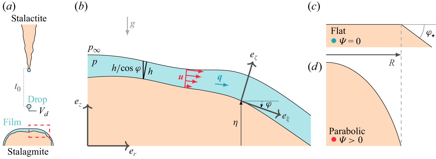
 Vd
 t0
 h(ξ)
 (r,z)
 η(r)
 φ(ξ)
 (ξ,ζ)
 p(ξ,ζ)
 p∞
 u(ξ,ζ)
 q(ξ)
 g
 Ψ=0
 R
 φ⋆
 Ψ>0
 r∈[0,R]
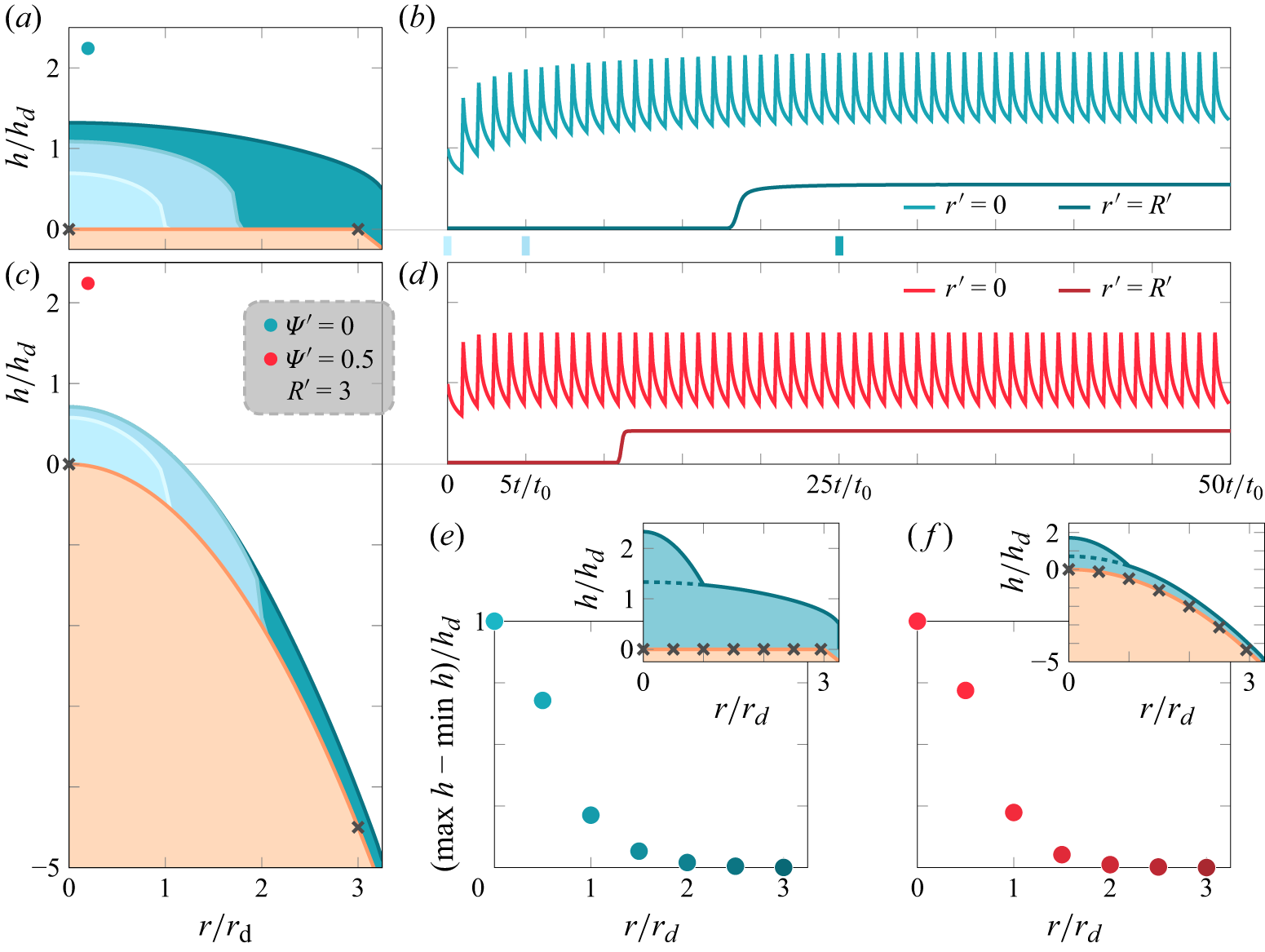
 Ψ′=0
 Ψ′=0.5
 t0′=1
 r′=0
 R′=3
 hs′(r′)
 (t′=kt0′−,k∈N)
 t0=1
 R′=5
 Ψ′=0
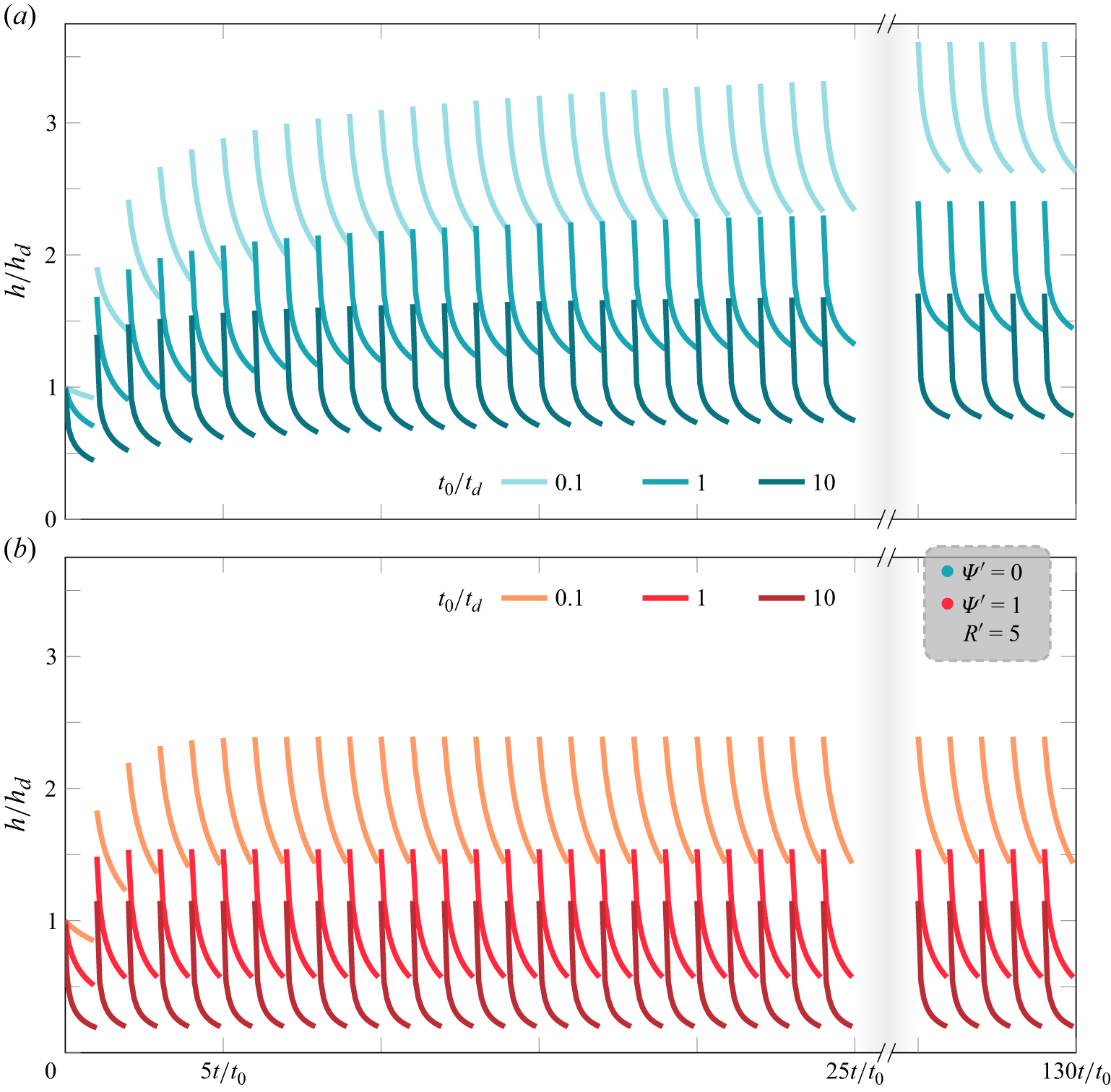
 Ψ′=0
 Ψ′=1
 R′=5
 t0′=0.1
 t0′=10
 t0′=0.1
 t0′=1
 t0′=10
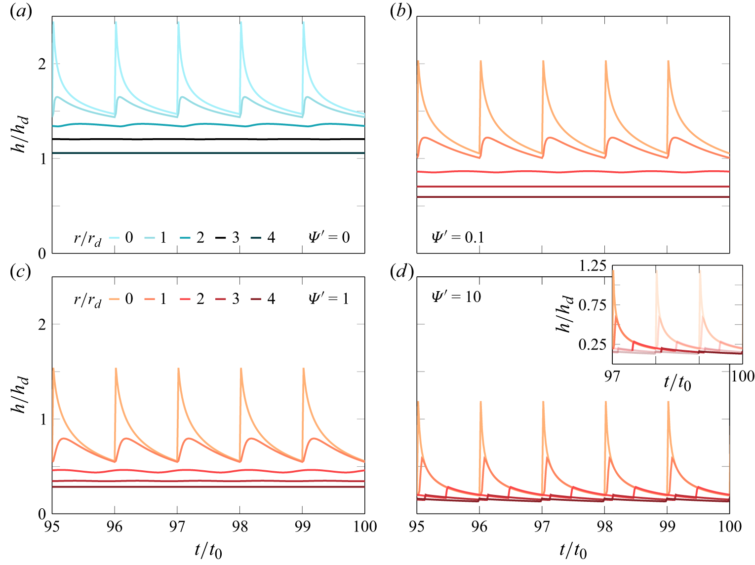
 t0′=1
 r′∈{0,1,2,3,4}
 R′=5
 Ψ′=0
 Ψ′=0.1
 Ψ′=1
 Ψ′=10
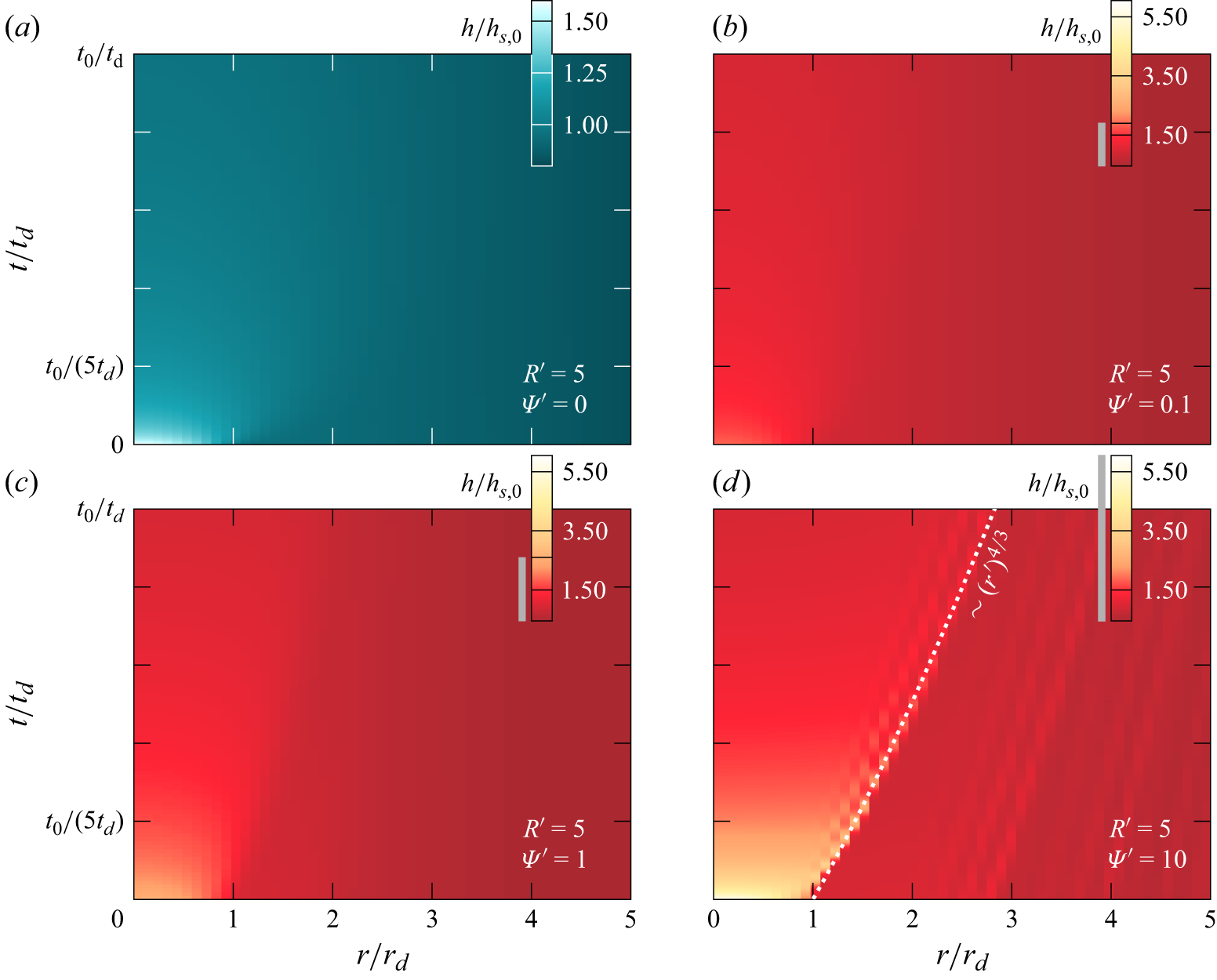
 h/hs,0
 t0′=1
 R′=5
 Ψ′=0
 Ψ′=0.1
 Ψ′=1
 Ψ′=10
 ∼0.6
 h/hs,0<1
 ∼(r′)4/3
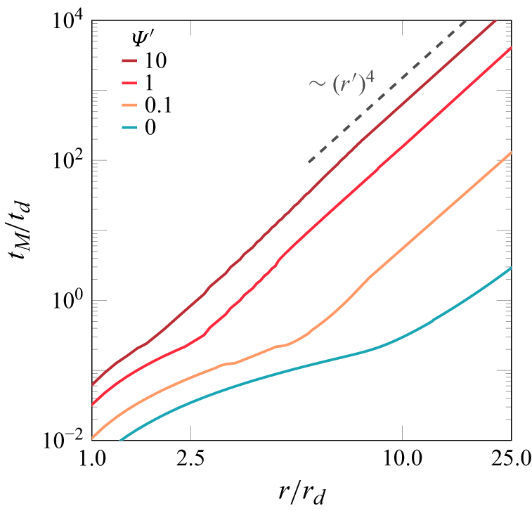
 t0′=1
 R′=5
 Ψ′=0
 Ψ′=0.1
 Ψ′=1
 Ψ′=10
 tM′∼(r′)4
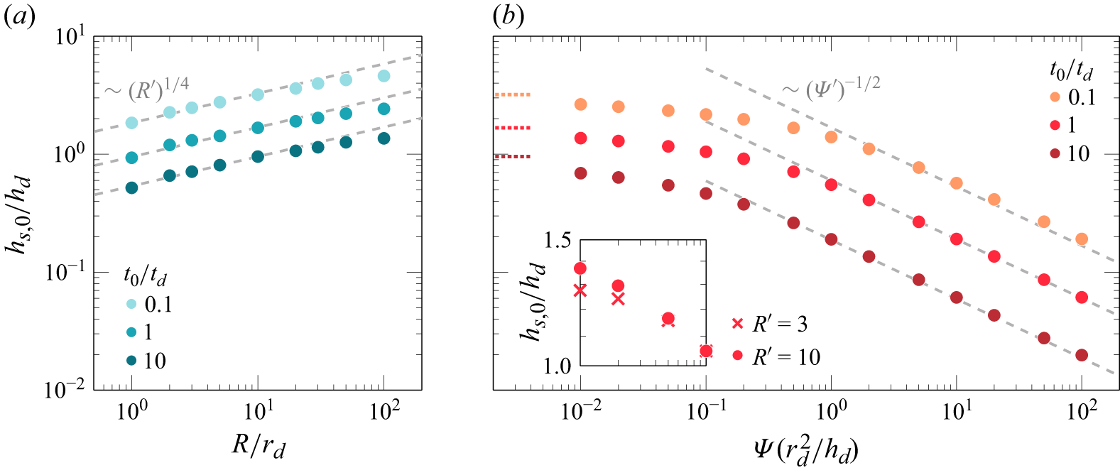
 hs,0/hd
 R′
 Ψ′
 R′=10
 hs,0′∼R′1/4
 hs,0′∼Ψ′−1/2
 Ψ′≲1
 R′=10
 Ψ′≪1
 hs
 Ψ′
 Ψ′=0.01
 Ψ′≪1
 t0′=1
 R′=3
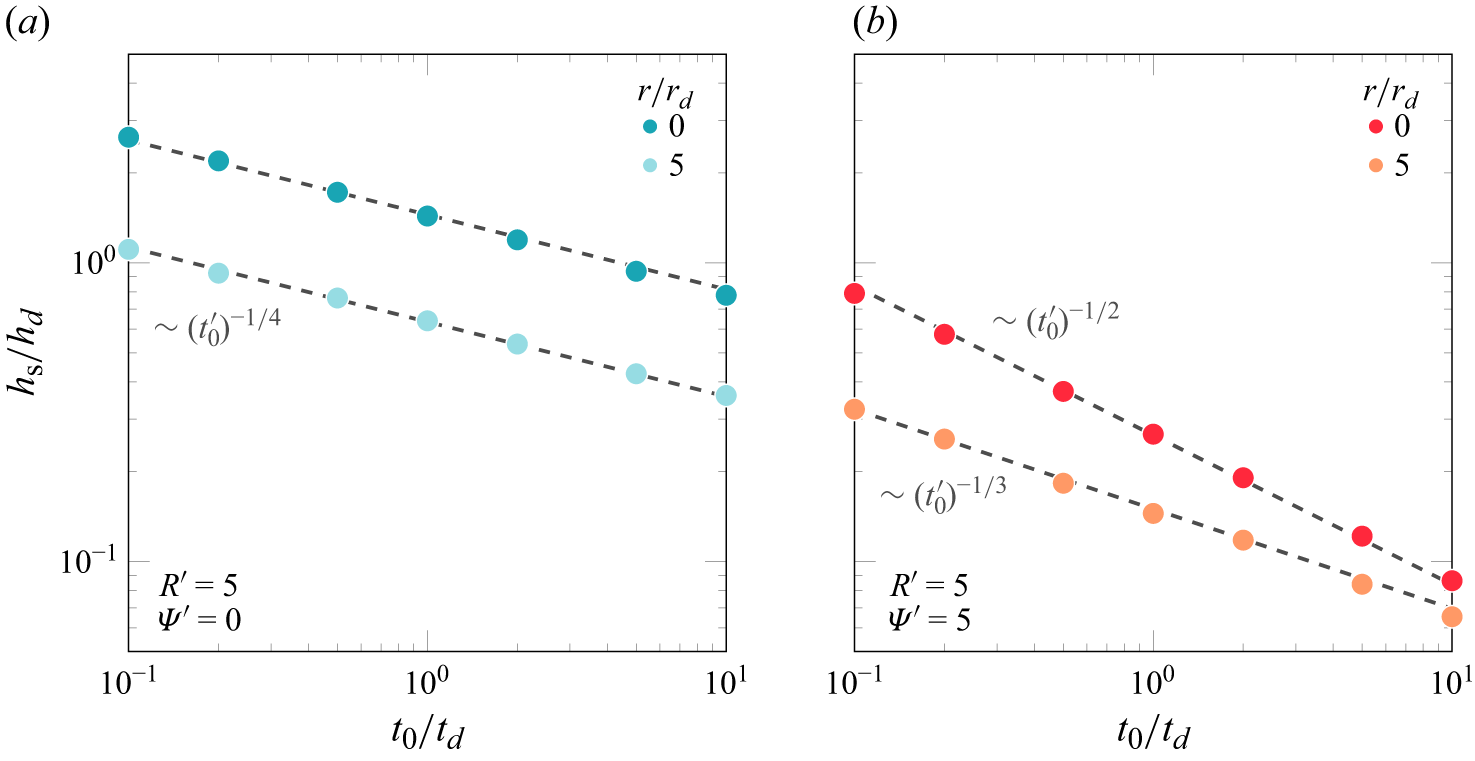
 hs/hd
 r′=0
 r′=5
 R′=5
 Ψ′=0
 Ψ′=5
 r=0
 ∼(t0′)−1/4
 ∼(t0′)−1/2
 r→R
 ∼(t0′)−1/4
 ∼(t0′)−1/3
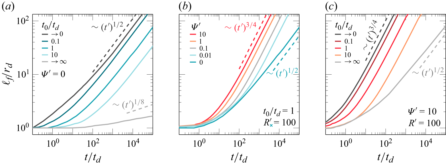
 Ψ′=0
 Ψ′=0
 Ψ′=10
 t0′→0
 t0′→∞
 t0′
 ℓf′
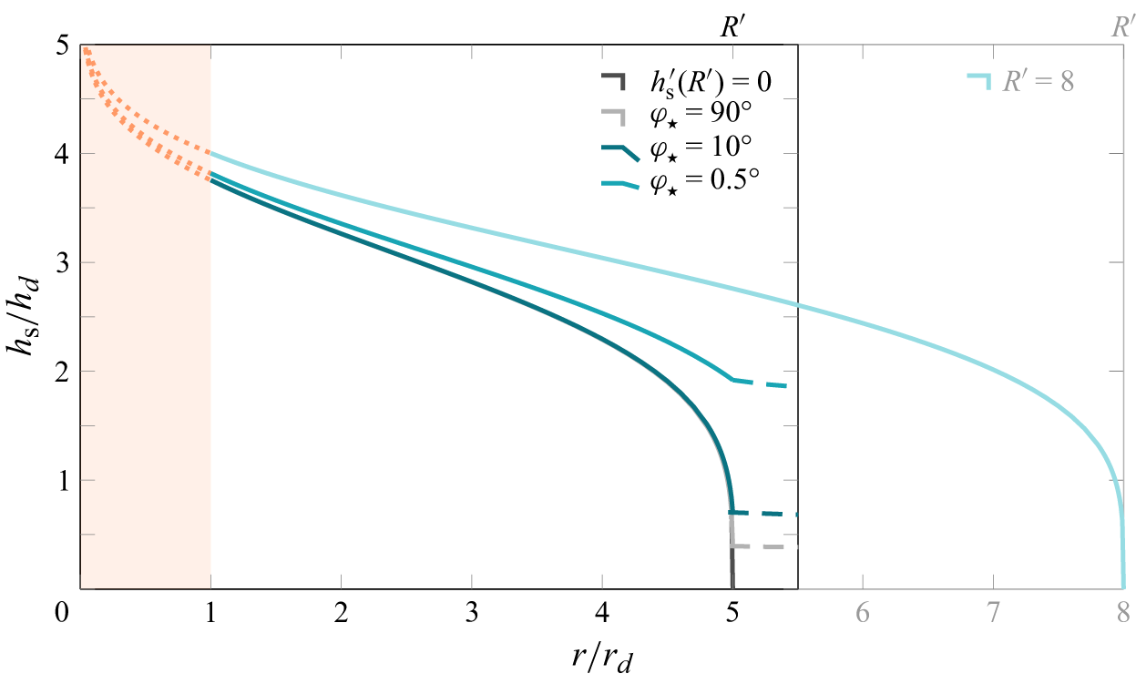
 R′=5
 r′=1
 r′→0
 φ⋆
 φ⋆=90∘
 10∘
 0.5∘
 hs′∼(r′)−1/3
 r′⩾R′
 hs′(R′)=0
 R′=5
 r⩾5.5cm
 hs(R)=0
 R=8cm
 r<1
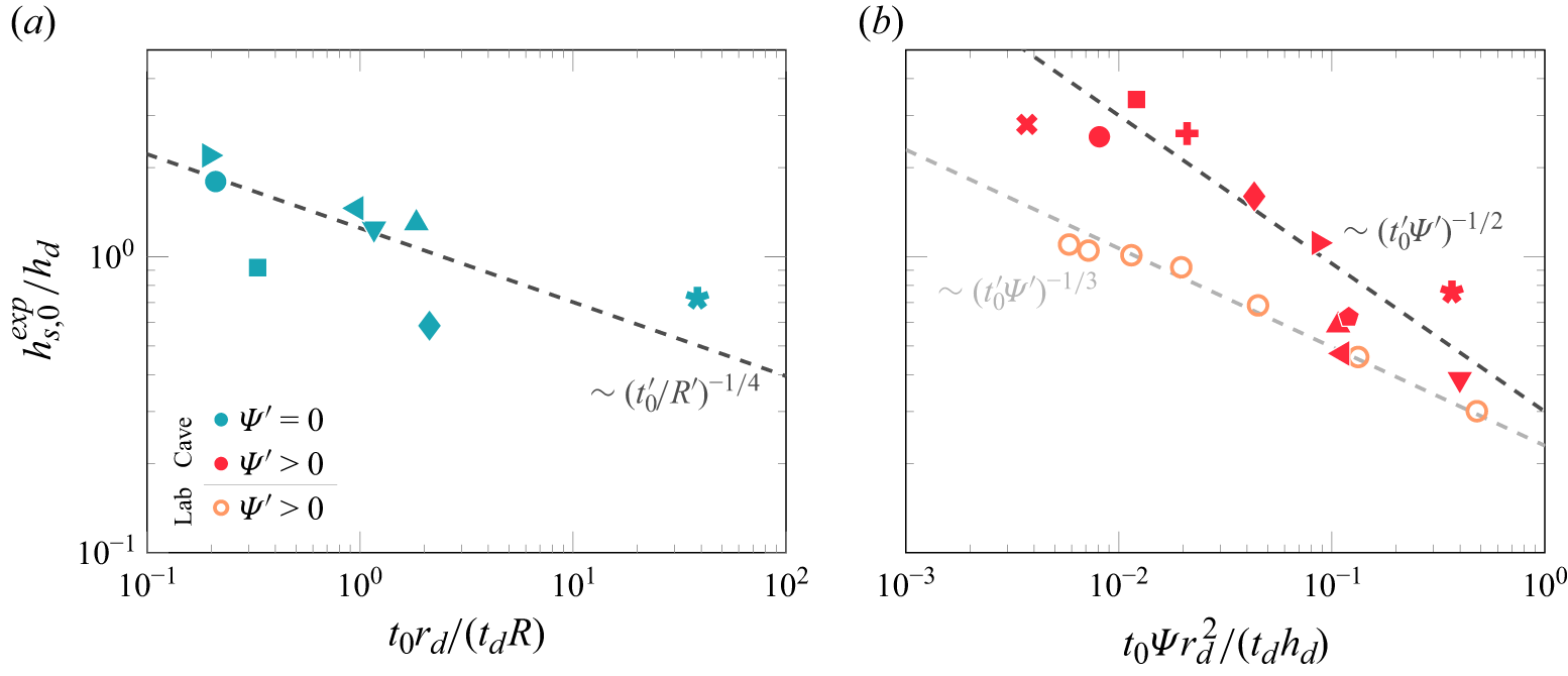
 t0′/R′
 t0′Ψ′
 ∼(R′)1/4
 ∼(t0′)−1/4
 ∼(t0′Ψ′)−1/3
 ∼(t0′Ψ′)−1/2
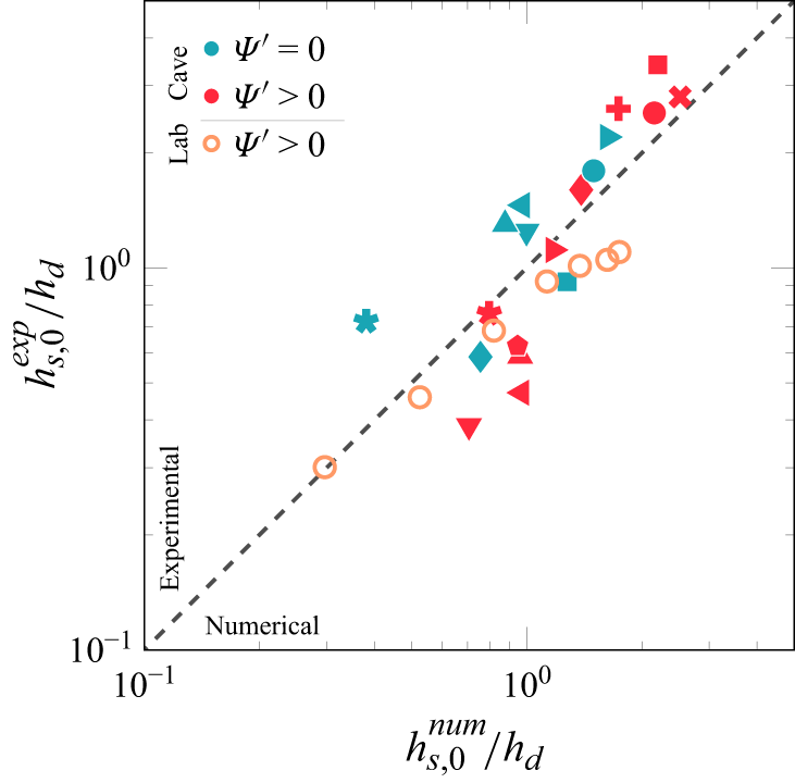
 t0′
 R′
 Ψ′
 hs,0′
 R′
 Ψ′
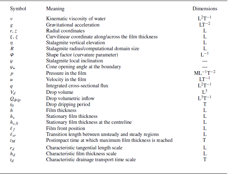
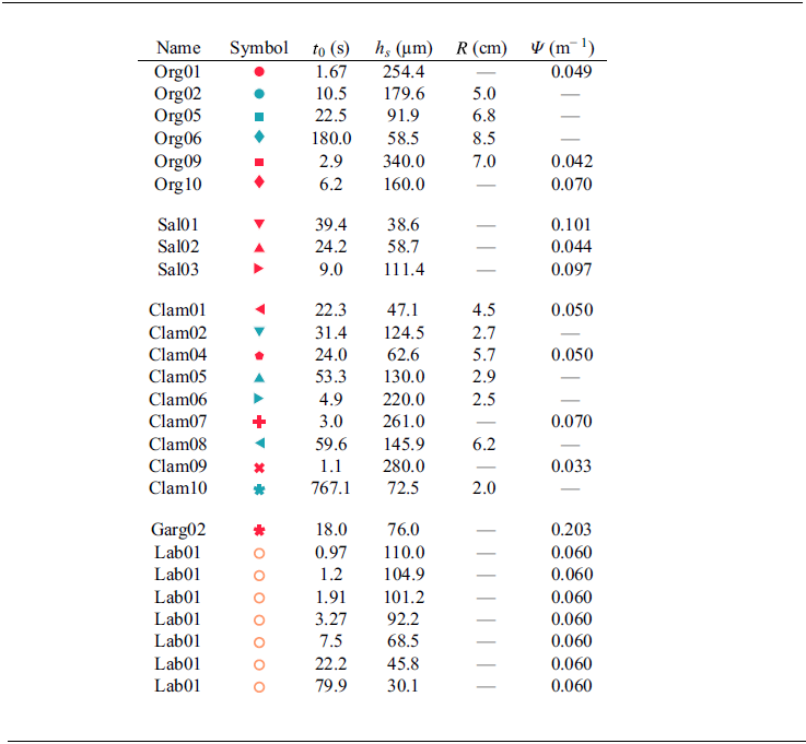
 ≲10%



