Introduction
Around the South Shetland Islands, lying just north of the Antarctic Peninsula (Fig. 1), the physical, chemical, and biological properties of the water column change considerably between coastal and open ocean areas during midsummer (Holm-Hansen & Hewes Reference Holm-Hansen and Hewes2004). The outflow of iron-rich, saline, and deeply mixed shelf waters from the Weddell Sea abut iron-poor, fresher, and shoaling Antarctic Surface Waters of the Drake Passage Antarctic Circumpolar Current (ACC). In the surface layer, waters of these two contrasting high nutrient and low chlorophyll (HNLC) areas mix, resulting in high iron, shoaled conditions at intermediate salinities that are optimal for primary production. Consequently, chlorophyll a (Chl a) concentrations have a “bell shaped” (unimodal) distribution when plotted against salinity (Hewes et al. Reference Hewes, Reiss, Kahru, Mitchell and Holm-Hansen2008). The interannual variability in maximal Chl a concentrations is largely a function of depth for the upper mixed layer (UML), and not in variations of the iron supply (Hewes et al. Reference Hewes, Reiss and Holm-Hansen2009). This South Shetland Islands area represents a region of natural Fe-fertilization (Hopkinson et al. Reference Hopkinson, Mitchell, Reynolds, Wang, Selph, Measures, Hewes, Holm-Hansen and Barbeau2007), with biogeochemical provinces that encompass contrasting biological limits (light and iron) and changing gradient between them. Smetacek et al. (Reference Smetacek, Assmy and Henjes2004) hypothesized that iron-replete versus iron-limiting biogeochemical provinces of the Southern Ocean are identifiable by the type of mortality (“krill” associated communities vs “salp” associated communities, respectively) encountered within the food web. If this occurs, environmental controls of different biogeochemical provinces might be reflected in the microbial trophodynamics that shape the composition of the phytoplankton community. The South Shetland Islands area therefore affords a natural setting to test such hypotheses.
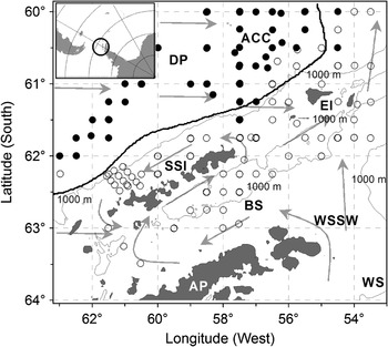
Map of the survey area showing locations where size-fraction Chl a samples were obtained. Generalized circulation for surface waters (grey arrows) with waters originating as outflow from the Weddell Sea (WS) crossing the shelf of the Antarctic Peninsula (AP) to become Weddell Sea Shelf Water (WSSW). This WSSW flows as a counter-current into the Bransfield Strait (BS) along the northern peninsular shelf (the 1000 m isopleth drawn as thin lines). At the south-western entrance of the Bransfield Strait, the current reverses to flow alongside the South Shetland Islands and out of the strait primarily north and north-east of Elephant Island (EI). Counter currents also occur along the shelf and shelf break of the continental margin north of the islands. The predominant current is the Antarctic Circumpolar Current (ACC) in the Drake Passage (DP) where iron is controlling phytoplankton biomass. The heavy line shows the boundary between productive coastal and Fe-controlled ACC waters from a multi-year dataset (Holm-Hansen & Hewes Reference Holm-Hansen and Hewes2004). Locations of CTD stations where size classed Chl a data were obtained either from ACC (solid symbols) or coastal (open symbols) waters in the study area are indicated; this convention for symbols is maintained for all figures that follow. The insert shows the study area in relation to Antarctica and South America.

Picoplankton (< 2 μm spherical diameter) have been reported to comprise 10–20% of the total phytoplankton in the summertime Southern Ocean (Fiala et al. Reference Fiala, Semeneh and Oriol1998, Kawaguchi et al. Reference Kawaguchi, Shiomoto, Imai, Tsarina, Yamaguchi, Noiri, Iguchi and Kameda2000, Hoffmann et al. Reference Hoffmann, Peeken, Lochte, Assmy and Veldhuis2006), although reports of 30–60% (Shiomoto et al. Reference Shiomoto, Kawaguchi, Imai and Tsuruga1998, Kawaguchi et al. Reference Kawaguchi, Ichii and Naganobu1999, Gall et al. Reference Gall, Boyd, Hall, Safi and Chang2001, Fiala et al. Reference Fiala, Machado and Oriol2002) are found. While Synechococcus is found in the Southern Ocean, its biomass becomes negligible in cold waters south of the Polar Front (Marchant et al. Reference Marchant, Davidson and Wright1987), being rarely, if at all, observed in the northern and western Antarctic Peninsula area (Holm-Hansen et al. Reference Holm-Hansen, Mitchell, Hewes and Karl1989, Hewes et al. Reference Hewes, Sakshaug, Holm-Hansen and Reid1990, unpublished observations). Nanoplankton (2–20 μm spherical diameter) generally account for an additional 25–75% of total eucaryotic microbial biomass (Hewes et al. Reference Hewes, Holm-Hansen and Sakshaug1985, Reference Hewes, Sakshaug, Holm-Hansen and Reid1990, Becquevort Reference Becquevort1997). A vibrant microbial predator-prey community occurs in the Southern Ocean (Hewes et al. Reference Hewes, Holm-Hansen and Sakshaug1985, Smetacek et al. Reference Smetacek, Assmy and Henjes2004) that is distinct from the classical “diatom-to-krill-to-whales” paradigm (Hart Reference Hart1942). Today’s paradigm is that phytoplankton size classes increase proportionally with crop size (Hewes et al. Reference Hewes, Holm-Hansen and Sakshaug1985, Reference Hewes, Sakshaug, Holm-Hansen and Reid1990, Chisholm Reference Chisholm1992, Varela et al. Reference Varela, Fernandez and Serret2002) resulting from the trophodynamic tradeoffs between of being small sized to provide growth efficiency at high predation cost, or of being large with slower growth rate but escaping microbial grazing (Thingstad & Sakshaug Reference Thingstad and Sakshaug1990, Thingstad Reference Thingstad1998, Smetacek Reference Smetacek1999, Smetacek et al. Reference Smetacek, Assmy and Henjes2004). Conceptually, two exclusive communities consume phytoplankton in the Southern Ocean: the classical food chain encompassing “diatom-to-krill-to-whales” communities (Hart Reference Hart1942; other zooplankton included, see Smetacek et al. Reference Smetacek, Assmy and Henjes2004), vs the microbial food web, in which protozoan grazers represent ∼30% of total eucaryotic microbial biomass (Hewes et al. Reference Hewes, Sakshaug, Holm-Hansen and Reid1990, Becquevort Reference Becquevort1997) and consume 20–80% of daily primary productivity (Becquevort Reference Becquevort1997, Hall & Safi Reference Hall and Safi2001, Selph et al. Reference Selph, Landry, Allen, Calbet, Christensen and Bidigare2001, Froneman et al. Reference Froneman, Pakhomov and Balarin2004).
Both bottom-up (i.e. light and nutrients) and top-down (i.e. grazing) factors probably structure the size distributions within the phytoplankton community (Smith & Lancelot Reference Smith and Lancelot2004, Hoffmann et al. Reference Hoffmann, Peeken and Lochte2007). In the South Shetland Islands area, the two contrasting HNLC areas found during summer define limits for phytoplankton biomass at high (light-controlled) and low (iron-controlled) salinity waters (Hewes et al. Reference Hewes, Reiss and Holm-Hansen2008, Reference Hewes, Reiss, Kahru, Mitchell and Holm-Hansen2009). With different biogeochemical provinces contrasted in relation to salinity for this area, the grazer community, and therefore the mortality environment for phytoplankton, might also be understood. I hypothesize that the spectrum for phytoplankton cell-size changes across the salinity gradient to reflect different environments of grazing mortality as encountered by microbial populations.
Materials and methods
Procedures
Size classed Chl a data were primarily collected during the Antarctic Marine Living Resources (AMLR) cruise aboard the RV Yuzhmorgeologiya (1999–2007) near the South Shetland Islands (Fig. 1). Data were collected during summer, when two ∼14-day surveys of the same area were made between mid-January and early March (only one survey was made in January 2007). In addition, samples were obtained during February–March 2004 aboard the RV L.M. Gould in the AMLR survey area, with stations for ACC and coastal waters temporally done in an unorganized manner. These stations were compared with average (and standard deviation) conditions for the South Shetland Area as measured over the 18 years 1990–2007 (Hewes et al. Reference Hewes, Reiss and Holm-Hansen2009).
Water samples were obtained from 8- or 10-litre General Oceanics water sample bottles attached to a rosette with Conductivity Temperature Depth (CTD) sensors. SeaTek (before 2007) and Chelsea (AquaTrack 2007) profiling fluorometers measured in situ fluorescence. Water bottles were fired at 11 standard target depths (5, 10, 15, 20, 30, 40, 50, 75, 100, 200, 750 m) or within 10 m of the seabed. Size fraction data reported here were only of bottle samples taken from the upper mixed layer (UML, samples taken at ≤ 30 m), with UML measured as the depth where potential density (sigma theta) is ≤ 0.05 kg m-3 of the surface value (Hewes et al. Reference Hewes, Reiss and Holm-Hansen2008, Reference Hewes, Reiss, Kahru, Mitchell and Holm-Hansen2009). CTD and associated sensor data were binned at 1 m intervals. Waters of the Drake Passage ACC have a temperature minimum (<∼0.5°C) with salinity of ∼34 that occurs at 75–125 m (the winter water remnant). This distinguishes them from coastal waters in the area that have a warmer (>∼0°C) and more saline temperature minimum, if any at all (Holm-Hansen et al. Reference Holm-Hansen, Hewes, Villafañe, Helbling, Silva and Amos1997, Holm-Hansen & Hewes Reference Holm-Hansen and Hewes2004). Size-fraction stations were classified as either of the “ACC” (Water Zone 1; see Hewes et al. Reference Hewes, Reiss, Kahru, Mitchell and Holm-Hansen2008), with winter water present in the water column, or “coastal” in which the winter water remnant was not present or could not be identified.
Hydroscopic 47 mm polycarbonate membrane filters of 1, 2, 5, 10, and 20 μm pore sizes were used to obtain sample filtrates without vacuum as modified from Murphy & Haugen (Reference Murphy and Haugen1985; also see Li Reference Li1986). Filters were placed on a wetted filter base of either stainless steel (Millipore) or polystyrene (Nalgene) and filtrate (the size-fraction) collected in a clean glass or polycarbonate container. No pre-filtration was used. Filtration rates varied from seconds (20 μm pore) to several minutes (2 μm pore) to obtain 200–400 ml filtrate (Chl a analyses required only 100 ml subsample). Such volumes are appropriate for this area (i.e. Sheldon Reference Sheldon1972) in which maximum Chl a averages < 5 mg m-3 (Hewes et al. Reference Hewes, Reiss and Holm-Hansen2009). Use of low vacuum or gravity to obtain a quantitative picoplankton fraction appears clone-specific (Li Reference Li1986), yet ample evidence indicates that vacuum filtration will break cells and release cellular materials into the filtrate (Goldman & Dennett Reference Goldman and Dennett1985, Li Reference Li1990, Fahnenstiel et al. Reference Fahnenstiel, Lohrenz and Redalje1994). Preliminary testing of natural samples from the study area using 14C methods (see Fahnenstiel et al. Reference Fahnenstiel, Lohrenz and Redalje1994) found low vacuum to obtain 1 and 2 μm filtrate resulted in excessively high Chl a. Low vacuum applied for filters having > 5 μm pore diameter was found to produce rates of filtration that were hard to control. Although some time was required to obtain the 2 μm filtrate, it was not inconvenient when properly anticipated considering that a series of size-fractions were being obtained at the same time for Chl a. The < 1 μm size-fraction was eventually discontinued because of the time required to obtain sufficient sample for analysis.
Chl a concentrations in the water samples were determined by measurement of fluorescence after extraction in absolute, acid-free methanol (Holm-Hansen & Riemann Reference Holm-Hansen and Riemann1978). Sample volumes of 100–200 ml were filtered through glass fibre filters (Whatman GF/F, 25 mm) at low pressure (maximal differential pressure of 1/3rd atmosphere), and extracted in 10 ml of MeOH at 4°C in the dark for at least 12 hours. The samples were then shaken, centrifuged, and the clear supernatant measured for Chl a fluorescence before and after addition of two drops of 1.0 N HCl using a Turner Designs TD-700 fluorometer. The fluorometer was calibrated with Chl a (Sigma) with concentrations determined by spectrophotometer. Stability of the fluorometer was verified daily by use of a solid-state standard (Turner Designs). The resolution of this procedure is routinely 0.01–0.1 mg Chl a m-3 as compared with spectrophotometer (unpublished).
Fluorescence yield (FY) of the phytoplankton sample was determined from voltage of the in situ profiling fluorometer measured during the time that sample bottles were triggered. The FY was obtained by dividing log output voltage (mVolt) by log Chl a concentration (1000 x mg m-3) as determined by extraction in MeOH, such that

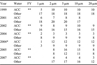
Years having FY are listed in Table I. Drake Passage ACC waters produce higher fluorescence yields than for coastal waters, and are used here as a proxy for conditions of iron-stressed phytoplankton communities (see Hewes et al. Reference Hewes, Reiss and Holm-Hansen2009 for details).
Years and type of water that samples were collected for Chl a size classes, and number of filtrates obtained for each filter pore diameter. Years with in situ profiling fluorometer data to estimate the fluorescence yield (FY) are indicated (**). Samples were obtained during AMLR surveys in the Elephant Island and South Shetland Islands area, with additional samples collected from the RSV L.M. Gould (2004*).

Data treatment and statistical methods
Values for size classes between 1 μm and 20 μm were obtained by subtracting Chl a concentrations from the filtrates of size-fractioned water for smaller membrane pore diameters from those of the next larger membrane pore diameter. The > 20 μm size class was obtained by the difference between the total Chl a and that of the 20 μm size-fraction filtrate. Occasionally, excessive concentrations occurred in a filtrate resulting in negative size class Chl a values (higher concentrations in a smaller membrane pore-size filtrate than its next larger membrane pore-size filtrate). Testing was carried out by the ratio of these negative values to the size-fraction filtrate from which they were obtained, with the size-fraction filtrate excluded if this ratio exceeded 5%. Of the 886 raw size class data,< 2% of size class data were excluded because of excessive concentrations in the size-fractioned filtrate (i.e. if the 2 μm fraction exceeded the 5 μm fraction, this would eliminate both 1–2 μm and 2–5 μm size classes), with remaining values resulting in negative ratios considered “zero” for the size class (i.e. insignificant differences that were below the resolution of methodology). Less than 0.5% of total data contained “zeros”, most of these being estimates of the> 10 μm size classes (i.e. there was no measurable difference between 10 μm or 20 μm size-fractions with the total). The < 5 and > 10 μm sizes were co-linear with the other size classes and considered redundant, and therefore were not considered for statistical analyses or discussed.
For practical purposes, “zero” values were assigned a value of 0.001 mg Chl a m-3 for statistical treatment involving logarithms. Regression statistics were carried out using a log-transformation on all Chl a concentration data (mg m-3 x 1000 = μg m-3, values of 0.001 become zero with log transformation) and compositions. Compositional data incorporated the logarithm of percent size class to total Chl a, with the logarithm used to straighten out inherent non-linearity for this type of data. Principal component analysis (PCA) and redundancy analysis (RDA) are statistical methods to examine linear and unimodal distributions of variables across gradients (ter Braak Reference Ter Braak1987), with these tests done here using CANOCO© version 4.53. For both PCA and RDA, linear regressions between the principal components (site scores) and salinity, UML depth, total Chl a, and fluorescence yield were used to determine their correspondence with the component axes. Only size class data was involved with PCA, whilst RDA incorporated size class data for “species” and total Chl a, salinity, UML depth, and fluorescence yield as environmental variables. A reduced matrix of size class data was used for both PCA and RDA that eliminated missing size class data. Since the < 1 μm size-fraction was the class least often obtained (Table I), both the< 1 μm and the 1–2 μm size classes were eliminated for multivariate analyses, so that a total of 117 stations formed the reduced data matrix. The log-ratio composition of stations was compared through linear regression with the site (component) scores for axes derived by PCA.
Results
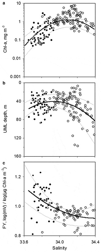
The subset of stations having size classed Chl a data can be compared with conditions within the South Shetland Islands area as averaged over an 18 year period. Total Chl a concentrations for size-fraction stations were distributed across the salinity gradient, having maximal values at salinities 34.0–34.2 (Fig. 2a). Depth of the UML shoaled from ∼80 m for high salinity waters to ∼40 m at intermediate salinities ∼34.0 (Fig. 2b). Fluorescence yields were generally low at salinities> 34.0 and became elevated at lower salinities (Fig. 2c). For the subset of station data, ACC waters occurred at salinities below ∼33.9, characterized by lower biomass, shallower UML depths, and high variability in fluorescence yields (a proxy measure of iron limitation) as compared with coastal waters. Coastal waters had higher Chl a concentrations, a relatively narrow range in fluorescence yields, and highly variable UML depths. The polynomial regression fit for Chl a, UML depth, and fluorescence yield (Table II; solid lines in Fig. 2) are shown within the bounds of standard deviations (± of the mean) covering the 18 year AMLR survey history (stippled lines in Fig. 2), and indicates that the subset of stations having size-fraction data was not unusual for the area.
Hydrographic and biological patterns across the salinity gradient. Distributions of a. total Chl a, b. UML depth, and c. fluorescence yield across the salinity gradient at stations where size class data were obtained, with ACC (solid symbols) and coastal (open symbols) samples indicated (see Fig. 1). Thick solid curves are 2nd order polynomial regressions, with statistical details provided in Table III, and thin stippled curves are upper and lower bounds for standard deviations of the 18 yr means as reported by Hewes et al. (Reference Hewes, Reiss and Holm-Hansen2009). Iron-rich, high salinity water enters the Bransfield Strait from the Weddell Sea (refer to Fig. 1), and becomes diluted by mixing as it flows toward iron-poor surface waters of the ACC. Maximal Chl a occurs at salinity ∼34 (a), and is where the UML has shoaled to shallow depths (b) removing light-limiting conditions before iron becomes depleted through phytoplankton assimilation and a dilution with the Antarctic Surface Water (salinities less than ∼34). Presumably low iron conditions in this Antarctic Surface Water increase the physiological stress on phytoplankton communities which is reflected in the higher fluorescence yields (c).

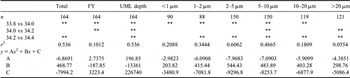
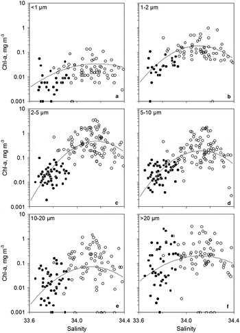
Statistical details for 2nd order polynomial regressions of total Chl a, Fluorescence Yield (FY) and UML depth against salinity plotted in Fig. 2, and for size classes plotted in Fig. 5. Chl a values were log transformed before regressions after multiplication by 1000 (e.g. μg m-3) to eliminate negative values. As a test for the significance of the modes for polynomial regressions drawn in Fig. 2, separate variance t-tests were used. Total Chl a concentrations were higher and both UML depth and fluorescence yields lower at binned salinities ± 0.1 in the middle of the salinity gradient compared with end members (P < 0.05, **). Similarly, size classed Chl a concentrations were tested to find significance of the modality for polynomial regressions plotted in Fig. 5. The r 2 and parameters for polynomial regressions drawn in Figs 2 & 5 are given.

Total Chl a concentration, UML depth, and fluorescence yield were tested for having a bell-shaped (unimodal) pattern in relation to the salinity gradient using separate variance t-tests (Table II); only fluorescence yield had no difference at salinities > 34.2. The interannual variability of total Chl a as collected over six field seasons (Table I) was considerable, with mean maximal concentrations (measured at salinities ranging 33.9–34.2) being highest in 2007 (4.7 mg Chl a m-3) and lowest in 2002 (0.9 mg Chl a m-3). The variability in this Chl a had little to do with station location, since median (± standard deviation) salinities as sampled from size-fraction stations were highest in 2007 (34.17 ± 0.16) and lowest in 2005 (33.85 ± 0.16), and compare with the other four years having a salinity of 33.98 ± 0.19. Therefore, the subset of stations for which size classed Chl a data was obtained represented averaged conditions within the South Shetland Islands area as compared with 18 years of survey history. Saline waters were deeply mixed and of low Chl a from light-controlling conditions. Fresher ACC waters also had low Chl a concentrations with relatively shallow mixing conditions, but biomass was probably controlled by iron, as indicated by elevated fluorescence yields.
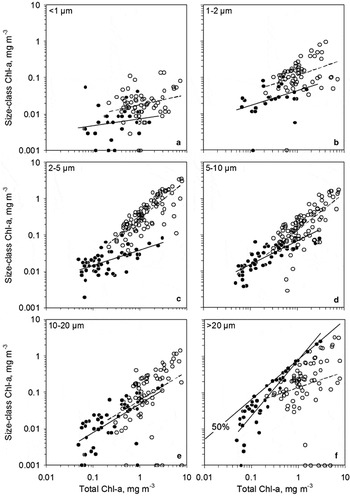
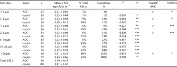
For both ACC and coastal waters, the Chl a of size classes increased in proportion with the total Chl a concentration (Fig. 3). This occurred for all size classes with the exception of the <1 μm size class from the ACC and the microplankton from coastal waters (Table III). The ranges for total phytoplankton biomass differed between ACC (< 0.1–2.3 mg Chl a m-3) and coastal waters (0.2–∼7.6 mg Chl a m-3), but overlapped sufficiently to compare the concentrations for size classes in relation to a gradient of total Chl a concentration. In relation to total concentrations, coastal waters contained more Chl a from the < 10 μm size classes (Fig. 3a–d), and the ACC had more Chl a for > 20 μm size classes (Fig. 3f). The < 1 μm size class was generally< 10% of the total chlorophyll concentrations (but ranged> 1 order of magnitude), with some clogging of these filters evidenced by the “zero” values for this size-fraction (Fig. 3a). The picoplankton (< 2 μm) ranged 0.01–2.2 mg Chl a m-3, with most of this contained in the 1–2 μm fraction, and contributed ∼18% on average to the total phytoplankton biomass for coastal waters (Table III). The two “zero” values for the 1–2 μm size class (Fig. 3b) did not result from a clogging of filter pores, but rather reflect that equal concentrations were measured in both 1 μm and 2 μm size-fractions. The < 2 μm size class increased significantly with total Chl a (Table III), indicating the variability of the < 1 μm filtrate was large with respect to the Chl a gradient (Fig. 3a).
Size classed vs total Chl a concentrations. The Chl a concentrations for different size classes vs total Chl a as was found in ACC (filled circles) and coastal (open circles) waters in the South Shetland Islands region (symbols as in Fig. 1). The picoplankton constitute a. < 1 μm, and b. 1–2 μm, nanoplankton the c–e. 2–20 μm, and microplankton f. the > 20 μm size classes. Lines for log-log regressions of ACC (solid lines) and coastal (dashed lines) waters are shown, with statistical details of the significance for the regressions and significance for differences between ACC and coastal waters provided in Table III. Thin solid line in f indicates 50% total biomass for the microplankton.

Statistical details for Chl a size classes in ACC and coastal waters, with their individual and cumulative contribution to the total Chl a concentration shown. Statistics of size classed Chl a concentration regressed linearly with total Chl a concentrations (r 2) of lines in Fig. 3 are given. Comparison of whether coastal waters had more (>) or less (<) size classed Chl a than ACC waters. The significance (ANOVA, P < 0.05 = *, P < 0.01 = **, P < 0.001 = ***) that Chl a concentration of the size class vs total Chl a concentration was different between ACC and coastal waters is given. For regression analyses, Chl a data were transformed by logarithm (mg Chl a m-3 x 1000 = μg m-3).

The microplankton (> 20 μm) fraction (Fig. 3f) contributed the largest portion to total Chl a of the ACC, but accounted for < 20% of the total on average in coastal waters (Table III). In coastal waters, nanoplankton generally contributed > 50% of the total Chl a (Table III), even at total concentrations > 7 mg Chl a m-3 (Fig. 3c–e). Most of the difference between ACC and coastal waters occurred in the contributions of the 2–5 μm (Fig. 3c) and the > 20 μm (Fig. 3f) size classes in relation to total Chl a concentrations. For coastal waters, the 2–5 μm size class had approximately five times more variability than found in ACC waters. The opposite occurred for the microplankton in which approximately five times more variability was found in ACC than coastal waters. It should be noted that “zero” values for the > 20 μm size class (Fig. 3f) resulted from equal Chl a concentrations being measured for the 20 μm filtrate as for the total.
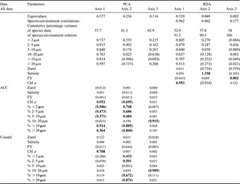
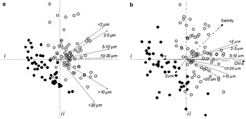
A PCA (using a reduced data matrix that contained no absences) resolved differences in size classed Chl a between ACC (n = 44) and coastal (n = 73) waters across both principal component axes (pc-) i and pc-ii (Table IV, Fig. 4a). For ACC and coastal waters combined, total Chl a concentration was correlated with principal components for pc-i (P < 0.001); pc-ii was correlated with salinity (P < 0.001) and ordered the size classes from small to large (Fig. 4a). In addition, the principal components for pc-i were distributed with modality in relation to salinity (2nd order polynomial: n = 117, r 2 > 0.49), reflecting the unimodal distribution of Chl a across salinity (Fig. 2a). Total Chl a was the only variable that was correlated with any axis when examined in relation to either ACC or coastal waters (Table IV). Although the total Chl a concentration from ACC stations was correlated with site scores (principal components) for both pc-i and pc-ii, the total Chl a concentration of coastal stations was only correlated with those for pc-i.
Details of PCA and RDA on size classed Chl a. Greater than 80% of the total variability (eigenvalues shown for “all data”) was explained by the first two PCA axes, and RDA resulted with a similar pattern of size classes eigenvectors as PCA, but aligned (in bold) with Chl a concentration as rd-i and with salinity as rd-ii. For each of ACC and coastal waters, r 2 for salinity, total Chl a concentration, depth of the UML, and fluorescence yield (FY), as well as log-ratio composition data of size classes (%), from linear regression with principal components (site scores) for each PC axis given. The most significant correlations are in bold, with insignificant correlations (P > 0.5) indicated by small print, and negative correlation by parentheses. Total Chl a concentration was correlated with pc-i for both coastal and ACC waters, but only the composition of size classes from the ACC were correlated with this axis. The composition of size classes from both ACC and coastal waters were correlated with pc-ii, but only total Chl a concentration from ACC waters was correlated with this axis.

Plots for multivariate analyses of size classed Chl a concentrations. a. Eigenvectors (small solid arrows) and site scores for a PCA upon a reduced matrix of size classed Chl a concentrations plotted across the first two axes (centred lines, each scaled to ± 1). Samples from the ACC (filled circles) are separated from those obtained from coastal waters (open circles). For the total data, Chl a was associated with pc-i (Table IV) that split size classes between nanoplankton and microplankton along pc-ii (eigenvectors for size classes as solid arrow lines). b. Redundancy analysis was done with the same reduced size class matrix, and included salinity, total Chl a concentration, UML depth (Zuml), and fluorescence yield (FY) as environmental variables (dashed arrow lines). For RDA, total Chl a concentration was associated with rd-i, and salinity associated with rd-ii, while fluorescence yield (less so with UML depth) was associated with rd-iii. For PCA and RDA, samples and size classed Chl a concentrations had a similar pattern in relation to component axes (centred lines, each scaled to ± 1, with axes labelled). Statistical details for both PCA and RDA are given in Table IV.

The RDA placed total Chl a, salinity, depth of the UML, and fluorescence yield in relation to each other (as multi-linear regressions) to describe a general environment that associated the variability of the different size classes (Fig. 4b, Table IV). The general pattern of size class eigenvectors and class of water obtained by PCA was maintained with RDA; total Chl a concentration represented the primary RDA axis (rd-) i, and salinity lay diagonal between rd-i and rd-ii, but was mostly associated with rd-ii (Table IV). Variability for fluorescence yield and UML depth were explained across rd-iii as opposing eigenvectors, but had little influence upon those relationships found among size classes (Table IV). Therefore most of the variability in the size class data (81%) was explained as a function of Chl a and its unimodal relation with salinity (e.g. Fig. 2a). High saline, low biomass waters contain a higher contribution from nanoplankton Chl a than those of low saline, low biomass conditions. A succession of size classes occurred in relation to the unimodal pattern of total Chl a across salinity proceeding from small to large with increasing total biomass and decreasing salinity.
The RDA (Fig. 4b) indicates that each size class reached a different maximum in Chl a across the second axis that corresponded with the salinity gradient (Table IV). Since Chl a (as well as site scores for both pc-i and rd-i) has a unimodal pattern across the salinity gradient (Table II, Fig. 2a), each of the size classes also does (Table II, Fig. 5). Although there was considerable variability of all size class Chl a in relation to salinity, the< 1 μm size-fraction only decreased at low salinity (P < 0.05), the 1–2 μm and nanoplankton had lower Chl a at both low and high salinities (P < 0.05), while microplankton increased from highest to mid salinity (P < 0.05) with no difference at low salinity (Table II). Indicated by both PCA and RDA is that the maximum Chl a concentration for each size class was reached at a different salinity (i.e. having a different salinity optimum), but this was not resolved simply by size class vs salinity plots (Fig. 5).
Size classed Chl a concentrations across the salinity gradient. Concentrations of Chl a for the different size classes across the salinity gradient, with regressions of 2nd order polynomial regressions drawn. Statistical details of these regressions, and tests of modality are given in Table II. a, b. Picoplankton, and c.–e. nanoplankton have a unimodal distribution across salinity, but f. the microplankton Chl a does not decline in a significant manner at salinities < 34. The loss of nanoplankton Chl a in ACC waters (c-e, solid symbols) accounted for most of the decrease of total Chl a at salinities < 34 (see Fig. 4). The small change in microplankton relative to the total decrease in Chl a across salinity (f) results with the positive relationship with total Chl a and higher contribution to the total in ACC waters (Fig. 3f).

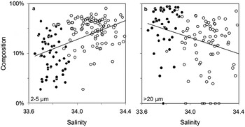
The community composition based on size classes changed differently for ACC and coastal waters in relation to both Chl a and salinity (Table IV). Total Chl a concentration for both ACC and coastal waters was correlated with pc-i. Yet, microplankton increased in composition (nanoplankton composition decreased) with the increase of total Chl a as correlated with pc-i only for ACC waters and not for coastal waters. However, microplankton (and inversely, nanoplankton) compositions were correlated with pc-ii for both ACC and coastal waters, but the total Chl a concentration for coastal waters was not correlated with pc-ii. The microplankton co-varied with total Chl a concentration and accounted for ∼50% of total variability in ACC waters for Chl a> 0.2 mg m-3, but there was no relationship for coastal waters (Fig. 3f). In contrast, the 2–5 μm size class contributed much less variability to total Chl a in ACC waters, whereas it provided most variability to total Chl a in coastal waters (Fig. 3c, Table III). Therefore samples from ACC and coastal waters were distinguished by PCA largely based on whether the community was dominated either by microplankton or the 2–5 μm size class (Fig. 6).
Changes in phytoplankton community composition across the salinity gradient. a. The 2–5 μm size class increased in percentage of total Chl a concentration across the salinity gradient between ACC and coastal waters, while b. the microplankton had the highest percentages of total Chl a concentration in ACC waters and lowest for coastal waters. Lines are linear regressions (P < 0.001) of log-ratio composition (including “zero” values for the > 20 μm size class) vs salinity. No other size class had a significant change in composition in relation to salinity, therefore not plotted.

Since total Chl a has a unimodal distribution in relation to salinity (Fig. 2a), so do the sum of its parts (Fig. 5) that make up the community composition. Yet most of the variability in the community composition occurred independently of Chl a concentration (i.e. across pc-ii and rd-ii), and was best described by the reciprocal relationship in composition between the microplankton and the 2–5 μm size class that occurred across the salinity gradient (Fig. 6). This resulted from the orthogonal relationship found for their eigenvectors (e.g. having independent variability) obtained by PCA and RDA (Fig. 4; Table IV). The negative linear correlation between the microplankton and the 2–5 μm size class compositions (Fig. 6, P < 0.001) defined a gradient (pc-ii) that corresponded with salinity (rd-ii). It was this second axis each of PCA and RDA that modelled the unimodal relationship for the sum of the total components (pc-i) that corresponded with total Chl a concentration (rd-i). Thus, Chl a for each of the size classes co-varied with total concentrations (except microplankton of coastal waters), and this condition provided the components describing the first axis of both PCA and RDA. The differences between the size classes as a function of their composition were sequenced by PCA and RDA as a second axis (independent of total Chl a) with small cells more important in saline waters and large cells more important in fresher waters.
Importantly, from size class data plotted in relation to salinity (Fig. 5a–e, Table II), the pico-and nanoplankton Chl a decreased significantly from mid to low salinity waters. But while microplankton tend to decrease at lower salinities (Fig. 5f), it was not significant (Table II). Therefore, the change in composition of the phytoplankton community in ACC waters was not because of a relative increase in microplankton as waters became more eutrophic (e.g. at higher salinity). Rather, as coastal waters mix with those of the ACC to elevate total Chl a, nanoplankton of the 2–10 μm size classes (Fig. 3c & d) increase at a rate faster than the microplankton (Fig. 3f). Upon collapse of the bloom with increased dilution by ACC waters (salinities below ∼34), a rapid decline of the 2–5 μm size class (Fig. 5c), with little change in the microplankton biomass (Fig. 5f), transforms the nanoplankton-dominated community of saline waters into a microplankton-dominated community for the ACC (Fig. 6). Since most of the total biomass of these ACC waters has become microplankton, most of the variability in Chl a associated with these pelagic waters is a function of microplankton (Fig. 3f) as well.
Discussion
During midsummer in waters of the South Shetland Islands region, different proportions of pico-, nano- and microplankton in the phytoplankton community characterized iron-controlled, low salinity ACC waters and light-controlled, high salinity coastal waters. Small cells composed ∼75% of the coastal bloom biomasses in mid salinity (∼34) waters, while large cells composed substantial fractions of low Chl a populations in the ACC. The picoplankton contributed ∼18% of total Chl a in coastal waters, but only ∼3% for ACC waters. Within coastal waters, > 2 mg Chl a m-3 was measured in each of 2–5 μm and 5–10 μm size classes, and both picoplankton and nanoplankton concentrations varied with total Chl a, while microplankton concentrations had little co-variability. In contrast, microplankton contributed ∼50% to total Chl a in presumably iron-controlled regions of the Drake Passage ACC to dominate its community composition. “Leaky” filters might exaggerate the importance of smaller size classes (Murphy & Haugen Reference Murphy and Haugen1985, Stockner et al. Reference Stockner, Klug and Cochlan1990) as reported in the literature. However, this and similar artefacts were probably insignificant for the results obtained here because 1) the 4–5 filtrates used to provide each size class were made independently of each other, 2) the sum of averaged size classes provided ∼100% of the total concentration (Table III), 3) the spectrum of cell size was different between ACC and coastal waters in relation to the total, and 4) the results were reproduced over several field seasons. Reported artefacts of size-fractionation would also not explain the relatively high proportion of microplankton Chl a found for ACC waters.
Phaeocystis colonies are rarely observed in the South Shetland Islands area, with the autotrophic microplankton consisting mostly of diatoms and dinoflagellates, while Cryptomonas sp., motile Phaeocystis, and small pennate diatoms often make up the bulk of the nano-phytoplankton (Kang & Lee Reference Kang and Lee1995, Villafañe et al. Reference Villafañe, Helbling and Holm-Hansen1995). My results are contrary to a popularized “nanoplankton dominated blue water, microplankton dominated bloom” scenario, and other investigations tend to substantiate this. Shelf waters of the South Shetland Islands have previously been reported to contain high nanoplankton proportions (Kang & Lee Reference Kang and Lee1995, Kawaguchi et al. Reference Kawaguchi, Ichii and Naganobu1999, Reference Kawaguchi, Shiomoto, Imai, Tsarina, Yamaguchi, Noiri, Iguchi and Kameda2000, Varela et al. Reference Varela, Fernandez and Serret2002). In contrast, microplankton have been reported as a major fraction (∼50%) of phytoplankton biomass for the HNLC Drake Passage ACC (Helbling et al. Reference Helbling, Villafañe and Holm-Hansen1991, Kang & Lee Reference Kang and Lee1995, Shiomoto et al. Reference Shiomoto, Kawaguchi, Imai and Tsuruga1998), as well as in other low Chl a and HNLC sectors of the Southern Ocean (Froneman et al. Reference Froneman, Pakhomov and Balarin2004, Ehnert & McRoy Reference Ehnert and McRoy2007, Lance et al. Reference Lance, Hiscock, Hilting, Stuebe, Bidigare, Smith and Barber2007). Such data are paradoxical for the general understanding of the importance of cell size in relation to Southern Ocean microbial food web dynamics (i.e. Hewes et al. Reference Hewes, Holm-Hansen and Sakshaug1985).
Unamended natural water incubations obtained from the iron-limited Drake Passage ACC (Helbling et al. Reference Helbling, Villafañe and Holm-Hansen1991, Hopkinson et al. Reference Hopkinson, Mitchell, Reynolds, Wang, Selph, Measures, Hewes, Holm-Hansen and Barbeau2007), as well as, large-scale Fe-fertilization experiments in Fe-controlled regions of the Southern Ocean (de Baar et al. Reference De Baar, Boyd, Coale, Landry, Tsuda, Bakker, Bozec, Barber, Brzezinski, Buesseler, Boye, Croot, Gervais, Gorbunov, Harrison, Hiscock, Laan, Lancelot, Law, Levasseur, Marchetti, Millero, Nishioka, Nojiri, van Oijen, Riebesell, Rijkenberg, Saito, Takeda, Timmermans and Veldhuis2005, Hoffmann et al. Reference Hoffmann, Peeken, Lochte, Assmy and Veldhuis2006, Lance et al. Reference Lance, Hiscock, Hilting, Stuebe, Bidigare, Smith and Barber2007); generally end with a higher proportion of microplankton upon Fe-addition than they began. Conceptually, it is not difficult to model the transformation from pico- to microplankton-dominated communities during bloom evolution upon release from limiting conditions (Thingstad & Sakshaug Reference Thingstad and Sakshaug1990, Thingstad Reference Thingstad1998), especially for a “simple” ecosystem such as the Antarctic (Hewes et al. Reference Hewes, Holm-Hansen and Sakshaug1985). Microbial grazing is a primary mechanism leading to survivorship of larger cell-size upon eutrophication (Thingstad & Sakshaug Reference Thingstad and Sakshaug1990, Thingstad Reference Thingstad1998), with a rate that a cell escapes predation comparable to an increase in growth rate (Smetacek Reference Smetacek1999, Smetacek et al. Reference Smetacek, Assmy and Henjes2004). The microbial food web differs from the classical primarily because protist grazers grow at rates similar to the prey, and contrasts with diatom bloom conditions that can exist spatially since they are distanced in time from zooplankton grazing (Cushing Reference Cushing1981). Furthermore, invoking models of microbial dynamics also predicts that the biomass of small cells will plateau with eutrophication (Chisholm Reference Chisholm1992) as a function of microbial grazing (Thingstad & Sakshaug Reference Thingstad and Sakshaug1990, Thingstad Reference Thingstad1998). No evidence for small cells reaching a plateau in biomass was found for the South Shetland Islands area, even at very high Chl a concentrations. Generally, size classed Chl a increased as a proportion of the total Chl a for both ACC and coastal waters, even though the phytoplankton community compositions were different.
Therefore, the microbial dynamics of the South Shetland Islands area are unusual because nanoplankton dominated blooms and microplankton dominated ACC waters. An expansion for collective knowledge of mechanisms is required to explain why. Both bottom-up (nutrients and light) and top-down (grazing) controls probably shape phytoplankton community size structure (Smith & Lancelot Reference Smith and Lancelot2004, Hoffmann et al. Reference Hoffmann, Peeken and Lochte2007) in the South Shetland Islands area. Protist grazing would tend to increase microbial cell size with release from a limiting condition (light or iron) leading to eutrophication (Thingstad & Sakshaug Reference Thingstad and Sakshaug1990, Thingstad Reference Thingstad1998). That the smaller of nanoplankton were the dominant size class in blooms surrounding the South Shetland Islands is explicable as a function of reduced grazing pressure upon them, a hypothesis supported by the extreme variability of microplankton Chl a concentration of the same blooms. Namely, selective removal of microplankton cells, both autotrophic and heterotrophic, would elevate the nanoplankton biomass.
Smetacek et al. (Reference Smetacek, Assmy and Henjes2004) suggested that the types of mortality experienced by communities differ between biogeochemical provinces. In the South Shetland Islands area, this would correspond with deeply mixed, iron-rich, saline waters from the Weddell Sea shelf as separated across the salinity gradient from the well lit, iron-poor waters of the ACC (Holm-Hansen & Hewes Reference Holm-Hansen and Hewes2004, Hewes et al. Reference Hewes, Reiss and Holm-Hansen2008, Reference Hewes, Reiss, Kahru, Mitchell and Holm-Hansen2009). It is possible that contrasting microbial community structures are a result of different grazing strategies from spatially distinct zooplankton associations in the South Shetland Islands area. Salpa thompsoni (Foxton) and associated zooplankters occur in unproductive Drake Passage Waters, which contrasts with Euphausia superba Dana, the Antarctic krill, and its representative community that are found in productive coastal waters (Pakhomov et al. Reference Pakhomov, Froneman and Perissinotto2002, Atkinson et al. Reference Atkinson, Siegel, Pakhomov and Rothery2004). Salps feed non-selectively by a feeding net, while krill are omnivorous microplankton grazers. Together (with their assemblages), the two species define the different mortality regimes between light-controlled and iron-controlled biogeochemical provinces as hypothesized by Smetacek et al. (Reference Smetacek, Assmy and Henjes2004).
The proportion of krill pigmented green from grazing phytoplankton and microplankton Chl a concentration in the South Shetland Islands area co-vary (Kawaguchi et al. Reference Kawaguchi, Ichii and Naganobu1999, Reference Kawaguchi, Shiomoto, Imai, Tsarina, Yamaguchi, Noiri, Iguchi and Kameda2000), being evidence that krill do not graze down the small-sized cells in a rapid manner. The omnivorous grazing of microplankton by krill (and assemblage) would lead to selective losses of large protist grazers in addition to large phytoplankton cells, and permit small nanoplankton to increase biomass (Hewes et al. Reference Hewes, Holm-Hansen and Sakshaug1985). But the microplankton domination in the iron-controlled waters of the ACC must result from a different mechanism than found for coastal waters. If microbial grazing is the mechanism forcing larger cell size, the high proportion of microplankton could indicate a non-selective grazing by salps. The hypothesis is that, in contrast to size selective grazing, a top grazer inflicting a uniform mortality rate independent of cell size would drive the microbial trophodynamic equilibrium towards a larger cell size; large cell size would effectively become the microbial nutrient sink by escape from the “microbial loop”. The different food web dynamics of iron-controlled vs light-controlled systems are complex to measure and analyse, prompting Smetacek et al. (Reference Smetacek, Assmy and Henjes2004) to suggest large-scale Fe-fertilization as a manner to examine them. The natural iron fertilization process that occurs in the South Shetland Islands area (Hopkinson et al. Reference Hopkinson, Mitchell, Reynolds, Wang, Selph, Measures, Hewes, Holm-Hansen and Barbeau2007, Hewes et al. Reference Hewes, Reiss and Holm-Hansen2008, Reference Hewes, Reiss, Kahru, Mitchell and Holm-Hansen2009) may provide a simpler manner to do so, where the salinity gradient is used to distinguish these different biogeochemical provinces.
Acknowledgments
This work was supported by the U.S. AMLR program, administered by the Antarctic Ecosystem Research Division at NOAA’s Southwest Fisheries Research Center, La Jolla, California, funded in part by the National Oceanic and Atmospheric Administration, U.S. Department of Commerce, under grant NA17RJ1231 (O. Holm-Hansen), and NSF Office of Polar Programs grant numbers: OPP0230433/ ANT0444134 (G. Mitchell). Thanks to O. Holm-Hansen and C.S. Reiss for comments, and the two anonymous reviewers for their questions and suggestions. Views contained herein are those of CDH and do not reflect those of NOAA, NSF, or any of their subsidiaries.