1. Introduction
Gravity-driven flows in porous media form a classical topic in fluid mechanics, spanning a broad range of geophysical applications. By analogy with viscous gravity currents (Huppert Reference Huppert1982; Ungarish Reference Ungarish2020; Zheng & Stone Reference Zheng and Stone2022; Di & Huppert Reference Di and Huppert2024), porous medium gravity currents can be effectively modelled using low-dimensional, macroscopic sharp-interface approximations based on Darcy’s law (Huppert & Woods Reference Huppert and Woods1995; Lyle et al. Reference Lyle, Huppert, Hallworth, Bickle and Chadwick2005; Huppert & Neufeld Reference Huppert and Neufeld2014; Farahani et al. Reference Farahani, Chiapponi, Longo and Di Federico2024; Di et al. Reference Di, Huang, Quintard and Huppert2025). The fundamental two-dimensional propagation over flat topography is governed by (Huppert & Woods Reference Huppert and Woods1995)
 \begin{equation} \frac {\partial h}{\partial t} - \gamma \frac {\partial }{\partial x}\! \left ( h \frac {\partial h}{\partial x} \right ) = 0, \end{equation}
where
 $h(x,t)$
denotes the current height and
 $\gamma = \Delta \rho g K /(\phi \mu )$
represents the characteristic velocity arising from the buoyancy–viscous force balance. Therein,
 $\Delta \rho$
is the density contrast between the injected and ambient fluids,
 $g$
is gravity,
 $K$
is the permeability of the porous medium,
 $\phi$
is the porosity and
 $\mu$
is the dynamic viscosity of the injected fluid.
During propagation of porous medium gravity currents, real geological topographies often exhibit undulating features shaped by tectonic processes (Woods Reference Woods2015; Whelan & Woods Reference Whelan and Woods2023). Early efforts to incorporate topography targeted monotonic profiles, such as power-law forms
 $f(x) = a x^n$
, revealed transitions between hydrostatic- and topography-dominated regimes (Pegler, Huppert & Neufeld Reference Pegler, Huppert and Neufeld2013). More recently, Di et al. (Reference Di, Huang, Quintard and Huppert2025) advanced this by formulating a low-dimensional framework for small-slope curvilinear surfaces, extending the foundational model of Huppert & Woods (Reference Huppert and Woods1995) to yield
 \begin{equation} \frac {\partial h}{\partial t} - \gamma \frac {\partial }{\partial x}\! \left [ h \left ( \frac {\partial h}{\partial x} + \frac {{\rm d} f}{{\rm d} x} \right ) \right ] = 0. \end{equation}
For typical wavy topography
 $f(x) = A[1 - \cos (\lambda x)]$
with
 $A\lambda \ll 1$
, this framework shows that constant-volume releases of viscous fluid are governed by the volume ratio of released fluid to the characteristic topography.
Despite these advances, critical gaps remain: the above approaches either address monotonic profiles (Pegler et al. Reference Pegler, Huppert and Neufeld2013) or constant-volume releases (Di et al. Reference Di, Huang, Quintard and Huppert2025), yet neglect the more general scenario of the interplay between varying topography and sustained injection. Moreover, essential fluid-loss mechanisms, i.e. uniform drainage, characterised by slow permeation through low-permeability substrates and localised leakage, involving escape via fissured zones, remain unexamined for wavy topography, which are able to reshape flow patterns profoundly (Pritchard Reference Pritchard2007; Woods & Farcas Reference Woods and Farcas2009; Neufeld et al. Reference Neufeld, Vella and Huppert2009, Reference Neufeld, Vella, Huppert and Lister2011; Yu, Zheng & Stone Reference Yu, Zheng and Stone2017). Thus, existing low-dimensional frameworks limit comprehensive predictions for complex subsurface environments.
This study bridges these gaps through a unified low-dimensional theoretical framework that extends the model of Di et al. (Reference Di, Huang, Quintard and Huppert2025) to constant-flux injection over wavy topography, while integrating uniform drainage and the localised leakage dynamics. These advances have direct implications for all applications involving gravity segregated flows: gas injection in aquifers, petroleum engineering, carbon dioxide (CO
 $_2$
) sequestration problems, etc. This is the case for the downward-propagating dense currents illustrated figure 1(a) and also applicable to upward-migrating buoyant plumes, such as the flow dynamics in CO
 $_2$
sequestration, with the characteristic velocity
 $\gamma = \Delta \rho g K/(\phi \mu )$
holding universally. In this latter case, the frame orientation has to be changed in figure 1(b), with the z-axis in the downward direction. In this paper, we will use the frame introduced in figure 1(a) for describing both situations. Specifically, for application to CO
 $_2$
sequestration, the framework is only suited to early-stage injection, when macroscopic sharp-interface assumptions hold for supercritical CO
 $_2$
beneath low-permeability cap rocks, laying the groundwork for subsequent long-term processes such as convective dissolution, mixing and mineralisation (Huppert & Neufeld Reference Huppert and Neufeld2014).
The paper is structured as follows: § 2 derives the low-dimensional model for constant-flux propagation, drainage and leakage; § 3 benchmarks the low-dimensional model against a macroscopic sharp-interface flow model that more closely captures the underlying physics; § 4 explores the dynamics of propagation, drainage and leakage; § 5 applies the theoretical framework to CO
 $_2$
sequestration; and § 6 summarises our findings.
Schematic diagrams. (a) Distribution of constant-flux porous medium gravity currents over wavy topography during propagation, drainage and leakage. (b) Early stage of supercritical CO
 $_2$
beneath low-permeability wavy cap rocks; the orange arrows indicate flow direction.

2. Methodology
2.1. Low-dimensional modelling
For two-dimensional propagation in a porous medium, the volume conservation for an injection at a constant flux per unit width
 $q$
satisfies
 \begin{equation} \phi \int _{0}^{x_{\!f}\left (t\right )} h{\rm d}x=qt, \end{equation}
where
 $x_{\!f}$
is the position of the current front. The left boundary condition at the injection point is derived as
 \begin{equation} \gamma h\left (\frac {\partial h}{\partial x}+\frac {{\rm d}f}{{\rm d}x}\right )_{x=0}=-q/\phi , \end{equation}
with the moving right boundary condition
 $h (x_{\!f},t ) =0$
and initial condition
 $h(x,0) = 0$
.
Assuming the substrate is permeable, characterised by permeability
 $K_s$
, porosity
 $\phi _s$
and thickness
 $b$
, the superficial velocity through the substrate,
 $v_{s}$
, is modelled following Acton, Huppert & Worster (Reference Acton, Huppert and Worster2001), which treats the substrate as hydrostatic and fully saturated, with a constant uniform pressure imposed at the top boundary, by
 \begin{equation} v_{s}=-\frac {K_{s}\Delta \rho g}{\mu b}(h+b). \end{equation}
Considering the continuous Darcy velocity at the interface between the porous medium and the substrate, and applying mass conservation with (1.2), we formulate the drainage model by
 \begin{equation} \frac {\partial h}{\partial t} - \gamma \frac {\partial }{\partial x}\! \left [ h \left ( \frac {\partial h}{\partial x} + \frac {{\rm d}f}{{\rm d}x} \right ) \right ] = -\frac {v_s}{\phi } = -\frac {K_{s}\Delta \rho g}{\mu b\phi } \left (h+b\right ). \end{equation}
Further restricting the permeable substrate to a localised fissured zone at
 $x_s$
(
 $x_{s}\gt 0$
) with a width
 $w$
, the leakage model is given by
 \begin{equation} \frac {\partial h}{\partial t}-\gamma \frac {\partial }{\partial x}\! \left [h\left (\frac {\partial h}{\partial x}+\frac {{\rm d}f}{{\rm d}x}\right )\right ]=-\psi (x)\frac {K_{s}\Delta \rho g}{\mu b\phi } \left (h+b\right ), \end{equation}
with an indicator function
 $\psi (x)$
activating leakage within the region
 $|x-x_s|\leqslant w/2$
(Neufeld, Vella & Huppert Reference Neufeld, Vella and Huppert2009), defined by
 \begin{equation} \psi (x) = \begin{cases} 1, & |x-x_{s}| \leqslant w/2 , \\ 0, & |x-x_{s}| \gt w/2 . \end{cases} \end{equation}
From a global perspective,
 $w$
approximates the horizontal projection of the fissured-zone width under small-slope conditions. The boundary and initial conditions for drainage/leakage are identical to those applied during pure propagation.
2.2. Non-dimensionalisation
For the typical wavy topography
 $f(x)=A[1-\cos (\lambda x)]$
, using characteristic scales
 \begin{equation} S_{x} = \lambda ^{-1},\quad S_{h} = \left ( \frac {q}{\gamma \phi \lambda } \right )^{1/2}\!, \quad S_{t} = \left ( \frac {\phi }{\gamma q \lambda ^3} \right )^{1/2}\!, \end{equation}
where
 $x=XS_{x}$
,
 $h=HS_{h}$
and
 $t=TS_{t}$
, we derive the unified, dimensionless low-dimensional model
 \begin{align}&\qquad\quad \frac {\partial H}{\partial T}-\frac {\partial }{\partial X}\! \left [H\left (\frac {\partial H}{\partial X}+ \frac {{\rm d}F}{{\rm d}X} \right )\right ]=-\psi (X) \xi (H+B), \end{align}
 \begin{align}& H\! \left (\frac {\partial H}{\partial X}+\frac {{\rm d}F}{{\rm d}X}\right )\mid _{X=0}=-1,\quad H\left (X_{\!F},T\right )=0,\quad H\left (X,0\right )=0, \end{align}
 \begin{align}&\qquad\qquad\qquad\qquad F(X) = \varepsilon (1 - \cos X), \end{align}
 \begin{align}&\qquad\qquad\qquad \psi (X) = \begin{cases} 1, & |X-X_{s}| \leqslant W/2 ,\\ 0, & |X-X_{s}| \gt W/2, \end{cases} \end{align}
 \begin{align}&\qquad\qquad B=b\!\left (\frac {\gamma \phi \lambda }{q}\right )^{1/2}\!, \quad X_{s}=x_{s}\lambda ,\quad W=w\lambda . \end{align}
Therein,
 $X_{\!F}$
is the moving current front,
 $F(X)$
is the wavy topography,
 $B$
is the substrate thickness,
 $X_{s}$
is the fissured-zone location and
 $W$
is the fissured-zone width, all dimensionless. Crucially, the dimensionless parameter
 $\varepsilon$
is defined as
 \begin{equation} \varepsilon = A\!\left (\frac {\gamma \phi \lambda }{q}\right )^{1/2}\!, \end{equation}
whose physical interpretation is the ratio of the topographic amplitude to the characteristic current thickness, quantifying the topographic intensity. For pure propagation (
 $\psi$
= 0),
 $\varepsilon$
completely characterises the flow dynamics: when
 $\varepsilon$
= 0, the case degrades into flat topography; when
 $0\lt \varepsilon \ll 1$
, the topographic effect is slight; when
 $\varepsilon \sim \mathcal{O}(1)$
, the topographic effect is moderate; and when
 $\varepsilon \gg 1$
, the dynamics is dominated by the topography.
Another crucial dimensionless parameter
 $\xi$
indicates the attenuation rate of the current height, i.e. the drainage/leakage intensity, defined as
 \begin{equation} \xi = \frac {\gamma }{K \phi } \frac {K_s}{b}\! \left ( \frac {\phi }{\gamma q \lambda ^3} \right )^{1/2}\! , \end{equation}
which represents the ratio of the characteristic flow time to the drainage/leakage time, quantifying the importance of drainage/leakage effects. Here,
 $\gamma /(K\phi )$
characterises the properties of the injected fluid, while
 $K_s /b$
quantifies the drainage/leakage capacity of the substrate or fissured zone. When
 $\xi$
= 0, the model corresponds to pure propagation.
For low-dimensional modelling, a wavy topography introduces multiple length scales that preclude similarity solutions. Accordingly, we develop a second-order Crank–Nicolson numerical scheme to resolve the coupled dynamics of propagation, drainage and leakage.
2.3. Macroscopic sharp-interface flow model
To evaluate the accuracy of our low-dimensional model, we used a general macroscopic sharp-interface model as a benchmark. This model, based on a volume-of-fluid (VOF) formulation with a Darcy term, is well suited to simulating porous medium gravity currents, where it accurately captures a sharp saturation front without requiring a full macroscopic multiphase flow model (e.g. generalised Darcy’s laws) (Carrillo, Bourg & Soulaine Reference Carrillo, Bourg and Soulaine2020; Di et al. Reference Di, Huang, Quintard and Huppert2025).
The key advantage of this macroscopic model is its higher physical fidelity when the sharp-interface condition holds. Unlike the low-dimensional model derived from depth-averaged equations, which inherently omits flow complexities, the macroscopic model resolves the full governing equations and thus incorporates subtle yet real physical effects, such as weak inertia and viscous shear, particularly near the bottom boundary and over topographic gradients. Although secondary to the main gravity-driven flow, these effects are sensitively captured, providing a robust reference for evaluating the low-dimensional model.
Using the characteristic length and time scales of the low-dimensional model and defining the aspect ratio
 $\epsilon = S_h / S_x$
, along with characteristic intrinsic velocity and pressure scales defined by
 $U_{\textit{ref}}=S_{x}/S_{t}$
and
 $P_{\textit{ref}}=\rho g S_{h}$
, the dimensional form of the macroscopic sharp-interface flow model is written as
 \begin{align}&\qquad\qquad \boldsymbol{\nabla} ^{*} \boldsymbol{\cdot }\textbf{U}^* = 0, \nonumber \\[-12pt]\end{align}
 \begin{align} \frac {\partial \textbf{U}^*}{\partial T} + \boldsymbol{\nabla} ^{*} \boldsymbol{\cdot }\left ( \textbf{U}^* \textbf{U}^* \right ) &= - \frac {1}{{\textit{Fr}}^2} \boldsymbol{\nabla} ^{*} P^* + \frac {1}{\textit{Re}} \boldsymbol{\nabla} ^{*2} \textbf{U}^* + \frac {\epsilon }{{\textit{Fr}}^2} \textbf{e}_g - \frac {\phi }{\textit{Re} \boldsymbol{\cdot }\textit{Da}} \textbf{U}^* \nonumber \\[3pt]&\quad + \frac {1}{\textit{Bo}} \boldsymbol{\nabla} ^{*} \boldsymbol{\cdot }\left ( \frac {\boldsymbol{\nabla} ^{*} S}{|\boldsymbol{\nabla} ^{*} S|} \right ) \boldsymbol{\nabla} ^{*} S, \\[-12pt]\nonumber \end{align}
 \begin{align} \frac {\partial S}{\partial T} + \boldsymbol{\nabla} ^{*} \boldsymbol{\cdot }( &\textbf{U}^* S) + \boldsymbol{\nabla} ^{*} \boldsymbol{\cdot }\left [ \phi S (1-S) C |\textbf{U}^*| \frac {\boldsymbol{\nabla} ^{*} S}{|\boldsymbol{\nabla} ^{*} S|} \right ] = 0, \end{align}
where the dimensionless intrinsic averaged velocity, pressure and dimensionless numbers (Reynolds, Froude, Darcy and Bond) are defined as
 \begin{align} \textbf{U}^*=\frac {\textbf{U}}{U_{\textit{ref}}}, \quad P^*=\frac {P}{P_{\textit{ref}}}, \quad \textit{Re} = \frac {\rho }{\mu } \sqrt {\frac {\gamma q}{\phi \lambda }}, \quad \textit{Fr} = \frac {\gamma \lambda }{\sqrt {g}}, \quad \textit{Da} = K \lambda ^{2}, \quad \textit{Bo} = \frac {\rho \gamma q}{\phi \sigma _{\textit{eff}}}. \end{align}
The parameter
 $S$
denotes saturation and
 $\sigma _{\textit{eff}}$
represents the effective surface tension, while
 $C$
is a compression coefficient to maintain numerical sharpness of the two-fluid interface. Within the framework of porous medium gravity currents, it is assumed that a capillary fringe does not exist, thereby setting
 $\sigma _{\textit{eff}} = 0$
, corresponding to an effectively infinite Bond number. This configuration is physically relevant under conditions of low Darcy and Reynolds numbers, where inertial effects are negligible. We implement the model numerically via computational fluid dynamics (CFD) within the open-source platform
 ${\textrm{OpenFOAM}}^{\circledR}$
.
3. Comparison between low-dimensional and macroscopic sharp-interface models
Comparison of experimental (Pegler et al. Reference Pegler, Huppert and Neufeld2013) and numerical profiles for constant-flux glycerol over an inclined bottom in a Hele-Shaw cell via the macroscopic sharp-interface flow model.

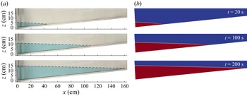
We first benchmark the macroscopic sharp-interface flow model against the experiment (Pegler et al. Reference Pegler, Huppert and Neufeld2013). As depicted in figure 2, the evolution at various times of glycerol injected at constant flux at the origin into a Hele-Shaw cell with an inclined bottom, with a gap thickness of 1.27 cm, corresponding to a cell permeability of
 $1.34 \times 10^{-5}$
m
 $^2$
, is reproduced by the macroscopic model in terms of fluid shapes. Furthermore, we compare the macroscopic CFD results at various Reynolds numbers with the similarity solution of the low-dimensional model for the front position of porous medium gravity currents over horizontal surfaces, given by
 $X_F = 1.48 T^{2/3}$
(Huppert & Woods Reference Huppert and Woods1995). As shown in figure 3(a), the two exhibit excellent agreement, with the macroscopic solution lying slightly below the similarity solution. This small difference stems from the comprehensive inclusion of fluid viscous effects in the macroscopic model, such as the formation of the current during initial injection, in contrast to the restriction of the low-dimensional model to viscous influences along the primary horizontal direction.
We now focus on a wavy topography, benchmarking the low-dimensional model against macroscopic CFD simulations in a two-dimensional domain filled with a homogeneous porous medium of porosity
 $\phi = 0.37$
and permeability
 $K = 6.8 \times 10^{-7}$
m
 $^2$
(Di et al. Reference Di, Huang, Quintard and Huppert2025). Three cases are considered, each featuring a fixed wavelength
 $2\pi / \lambda = 0.2$
m and amplitudes
 $A = 0.005$
,
 $0.01$
or
 $0.015$
m. To account for drainage and leakage, permeable wavy substrates underlie the bottom, with the same porosity
 $\phi _s = 0.37$
, uniform thickness
 $0.01$
m and three permeability values
 $K_s = 6.8 \times 10^{-9}$
,
 $3.4 \times 10^{-9}$
or
 $6.8 \times 10^{-10}$
m
 $^2$
. Boundary conditions include atmospheric pressure at the top, right and substrate outlet; symmetry at the left; and no-slip at the bottom. For leakage simulations, the permeable substrate is confined to the third wavelength region.
Comparison of low-dimensional and macroscopic sharp-interface models. (a) Validation of the macroscopic sharp-interface model against the similarity solution for fronts of porous medium gravity currents over flat surfaces. (b) Profile comparison of constant-flux glycerol–air porous media current during propagation, drainage and leakage over wavy topography (
 $\varepsilon$
= 0.24) at
 $Re$
= 0.43 and
 $T$
= 91.94; yellow lines show low-dimensional model solutions, red regions the macroscopic CFD results and black lines the permeable substrate (
 $B$
= 0.488;
 $Da$
=
 $6.7 \times 10^{-6}$
).

Comparison of front positions predicted by the low-dimensional and macroscopic sharp-interface models for constant-flux porous medium gravity currents under propagation, drainage and leakage. Panels show (a)
 $K/K_s = 100$
; (b)
 $K/K_s = 500$
and
 $1000$
. Solid lines denote low-dimensional model solutions; scatter points the macroscopic CFD results.

The domain is initially saturated with air, and glycerol (
 $\mu = 1.5$
Pa s,
 $\rho = 1.26 \times 10^3$
kg m
 $^{-3}$
) is injected at a constant flux at the origin. Figure 3(b) illustrates a representative comparison of current profiles from both models. In pure propagation, the profiles show excellent agreement. However, discrepancies emerge under drainage and leakage conditions, with the low-dimensional model underestimating propagation distances, most notably in leakage scenarios, where the underestimation intensifies further under drainage. Figure 4(a) quantifies the comparison by tracking current front positions across varying topographic intensities
 $\varepsilon$
in the three scenarios. For pure propagation, agreement persists robustly over time, confirming the validity of the low-dimensional model. By contrast, discrepancies under drainage and leakage grow progressively with time.
These discrepancies arise primarily from differences in sink-term formulations and underlying physical fidelity. The macroscopic model resolves the full transient two-phase dynamics within the substrate, capturing gradual imbibition and time-dependent saturation buildup that temporarily stores fluid and retards front propagation, namely an additional and transient mass-sink mechanism for the current. In contrast, the low-dimensional model employs a quasi-steady Darcy sink for both drainage and leakage, assuming instantaneous full saturation upon fluid arrival and immediate outflow, which over-drains the current and thus yields slower propagation. The cumulative error from this simplification scales with the spatial extent of the sink application, therefore the global drainage amplifies the discrepancy more than localised leakage confined to a narrow fissured zone.
To explore the influence of sink terms, figure 4(b) examines two additional cases with lower substrate permeabilities. As shown in the panel, the resulting drainage/leakage propagation distances exceed those displayed in figure 4(a). Moreover, this highlights that higher
 $K/K_s$
ratios mitigate the discrepancies in drainage/leakage propagation between the two models. This convergence stems from the fact that lower
 $K_s$
increases substrate hydraulic resistance, thereby reducing outflow and driving the dynamics toward the pure propagation. These observations underscore the utility of the low-dimensional model for high-contrast permeability scenarios between the porous medium and substrate.
A summary of the foundational assumptions of the low-dimensional model include a hydrostatic pressure distribution, Darcy’s law without inertial effect, a macroscopic sharp interface between the current and the ambient fluid, small topographic slopes on wavy topographies and a substantial permeability contrast between the porous medium and substrate. They together define the applicable regime of the present model and clarify its predictive scope for porous medium gravity currents over wavy substrates.
4. Dynamics of propagation, drainage and leakage
Now, we investigate the influence of the wavy topography using low-dimensional models. Figure 5(a) illustrates the effect of the topographic intensity
 $\varepsilon$
on the propagation delay factor
 $D$
, defined as
 $D = [( X_{F, {\textit{flat}}} - X_{F, {w\textit{a}v\textit{y}}})/ {X_{F, {\textit{flat}}}} ]\times 100\,\%$
, where
 $X_{F, {\textit{flat}}}$
and
 $X_{F, {w\textit{a}v\textit{y}}}$
represent the dimensionless front positions over flat and wavy topographies, respectively. The results show that
 $D$
oscillates in response to successive acceleration and deceleration phases as the current traverses the wavy profile. At low
 $\varepsilon$
(e.g.
 $\varepsilon = 0.1$
),
 $D$
fluctuates near zero, indicating negligible topographic influence. As
 $\varepsilon$
increases,
 $D$
shifts to positive values, reflecting a rise in topographic resistance due to enhanced viscous dissipation during uphill propagation.
To quantify topographic resistance, we analyse the underlying pressure gradients. The additional pressure gradient required to overcome the topographic slope scales as
 \begin{equation} \| \boldsymbol{\nabla }P_{\textit{topography}} \| \sim \Delta \rho g \left | \frac {{\rm d} f}{{\rm d} x} \right | \sim \Delta \rho g A \lambda , \end{equation}
while the characteristic viscous pressure gradient driving the flow scales as
 \begin{equation} \| \boldsymbol{\nabla }P_{{v\textit{iscous}}} \| \sim \frac {\mu \left |U\right |}{K} \sim \frac {\mu }{K} \frac {q}{\phi h}. \end{equation}
Using the characteristic height
 $S_h = ( q/\gamma \phi \lambda )^{1/2}$
and the definition of
 $\gamma = \Delta \rho g K / \mu$
, the ratio of the two scales simplifies to
 \begin{equation} \frac {\| \boldsymbol{\nabla }P_{\textit{topography}} \|}{\| \boldsymbol{\nabla }P_{{v\textit{iscous}}} \|} \sim A \left ( \frac {\gamma \phi \lambda }{q} \right )^{1/2} = \varepsilon . \end{equation}
This indicates that
 $\varepsilon$
directly represents the pressure gradient required to climb the slope to the characteristic viscous pressure gradient driving the flow, thereby formally establishing it as a quantitative measure of the topographic resistance.
Figure 5(b) illustrates the variation of topographic intensity
 $\varepsilon$
as a function of the characteristic flux
 $\sqrt {q\lambda /(\gamma \phi )}$
and topographic parameter
 $A\lambda$
. It reveals that
 $\varepsilon$
increases as the characteristic flux decreases and
 $A\lambda$
increases. In this plot, the range of
 $A\lambda$
satisfies the small-slope conditions for low-dimensional models (
 $A\lambda \ll 1$
), yet
 $\varepsilon$
can be significant – depending on
 $\sqrt {q\lambda /(\gamma \phi )}$
.
Propagation over wavy topography. (a) Temporal evolution of the propagation delay factor
 $D$
for topographic intensity
 $\varepsilon$
. (b) Range of topographic intensity
 $\varepsilon$
as a function of characteristic flux
 $\sqrt {q\lambda /(\gamma \phi )}$
and topographic parameter
 $A\lambda$
.

Regarding drainage, the system dynamics is governed by the combined effects of the topographic intensity
 $\varepsilon$
, the drainage intensity
 $\xi$
and the substrate thickness
 $B$
. To isolate and clearly elucidate the coupling between
 $\varepsilon$
and each of the other parameters, we selected relatively small, fixed values of
 $B = 0.02$
and
 $\xi = 0.1$
to minimise confounding influences. Figure 6(a) illustrates the interplay between
 $\xi$
and
 $\varepsilon$
under this constrained substrate thickness. The drainage intensity
 $\xi$
exerts a primary control on the maximum front position
 $X_{\textit{F, max}}$
, which decreases nearly linearly as
 $\xi$
increases. In contrast,
 $\varepsilon$
plays a secondary role: it promotes local fluid accumulation through topographic resistance, thereby enhancing downward drainage and further reducing
 $X_{\textit{F, max}}$
. Figure 6(b) examines the combined influence of
 $B$
and
 $\varepsilon$
at a fixed drainage intensity
 $\xi = 0.1$
. Both parameters significantly affect
 $X_{\textit{F, max}}$
. In summary, increases in topographic intensity and drainage intensity collectively strengthen local pressure gradients, promoting drainage fluxes and ultimately restricting the maximum propagation distance.
Drainage over wavy topography. (a) Combined effects of topographic intensity
 $\varepsilon$
and drainage intensity
 $\xi$
on the maximum propagation distance
 $X_{\textit{F, max}}$
. (b) Combined effects of topographic intensity
 $\varepsilon$
and substrate thickness
 $B$
on the maximum propagation distance
 $X_{\textit{F, max}}$
. Scatter plots represent the numerical results of the low-dimensional model and surfaces denote the fitting results.

Leakage over wavy topography. (a–c) Temporal evolution of sequestration efficiency
 $E_s$
at three representative fissured-zone locations. (d–f) Influence of fissured-zone location on the time
 $T_s$
required for sequestration efficiency to decline to thresholds; a longer
 $T_s$
indicates a longer duration of effective containment and thus better sequestration performance.

Leakage introduces additional complexity through the spatial characteristics of fissured zones, namely their location
 $X_s$
and width
 $W$
. The sequestration efficiency is quantified as
 $E_s = [ (Q_{\textit{injection}} - Q_{\textit{leakage}}) / Q_{\textit{injection}} ] \times 100\,\%$
(Neufeld et al. Reference Neufeld, Vella and Huppert2009). Figure 7(a–c) illustrates the temporal evolution of
 $E_s$
at three representative fissured-zone locations: the crest (
 $X_s = 5\pi$
), mid-downslope (
 $X_s = 5.5\pi$
) and trough (
 $X_s = 6\pi$
), under conditions of
 $\xi$
= 0.2 and
 $W$
= 2. Initially,
 $E_s$
remains at 100 % until the current reaches the fissured zone. Beyond this point,
 $E_s$
evolves distinctly depending on location: at the crest, efficiency increases with
 $\varepsilon$
at any given time, whereas at mid-downslope and trough positions, it decreases with increasing
 $\varepsilon$
. This demonstrates the crucial role of fissured-zone location for sequestration performance.
Figure 7(d–f) further examines how the fissured-zone position affects the time
 $T_{s}$
required to reach specific
 $E_s$
thresholds. As expected, fissured zones located further downstream delay the arrival of the current, thus increasing
 $T_{s}$
. At a high threshold (
 $E_s = 80\,\%$
), flat topography corresponds to the shortest
 $T_{s}$
, indicating the poorest sequestration. Increasing
 $\varepsilon$
prolongs
 $T_{s}$
, thereby enhancing sequestration. At lower thresholds (
 $E_s = 50\,\%$
and
 $10\,\%$
), topographic effects become more pronounced: crest locations continue to improve efficiency relative to flat topography, while trough locations degrade it. These differences fundamentally originate from variations in local current height, which govern the pressure gradients driving leakage. At crests, the wavy topography reduces current height compared with the flat case, lowering pressure gradients and leakage flux, thereby improving sequestration efficiency. Conversely, at troughs, the accumulation of fluid increases both pressure gradients and leakage, resulting in the poorest long-term sequestration performance.
5. Relevance to CO
 $_2$
geological sequestration

Application of low-dimensional model to supercritical CO
 $_2$
propagation, drainage and leakage beneath wavy cap rocks with various
 $A\lambda$
.

Finally, we illustrate this interest of low-dimensional models in conditions relevant to the early stages of CO
 $_2$
geological sequestration, focusing on plume propagation during injection while ignoring later processes like convective dissolution and residual trapping over thousand-year time scales. Although more detailed calculations of macroscopic models, such as Darcy–VOF simulations that omit inertial effects, would be needed to fully validate the low-dimensional approach under diverse geological conditions, it remains a practical tool for quickly assessing key trends in these scenarios.
The adopted geological parameters are drawn from representative field conditions: a density contrast of 500 kg m
 $^{-3}$
between supercritical CO
 $_2$
and ambient brine, a dynamic viscosity of
 $4 \times 10^{-5}$
Pa s, formation permeability of
 $3 \times 10^{-12}$
m
 $^2$
and porosity of 0.4 (Neufeld et al. Reference Neufeld, Vella and Huppert2009). For the cap rock, we assume the same porosity as the formation, a permeability four orders of magnitude lower, along with a uniform thickness of 10 m. The wavy cap rock is characterised by an amplitude
 $A = 5$
m, with a fissured zone of width 50 m.
We investigate the propagation of supercritical CO
 $_2$
beneath both flat and wavy cap rocks, considering small topographic parameters
 $A\lambda$
of 0.01, 0.02 and 0.03, as illustrated in figure 8. Figure 8(a) corresponds to a typical injected flux of the order of
 $10^{-2}$
m
 $^2$
s–1 (Neufeld et al. Reference Neufeld, Vella and Huppert2009). From the results, the front positions
 $x_{\!f}$
for pure propagation and leakage propagation are indistinguishable, whereas
 $x_{\!f}$
under drainage is markedly shorter. Also, the differences among the three wavy cap rocks are negligible. This is because the topographic intensities
 $\varepsilon$
at this injected flux are 0.043, 0.061 and 0.075, respectively, underscoring that the influence of wavy topographies remains minimal, yielding no discernible distinction of flow dynamics between flat and wavy cap rocks.
In contrast, figure 8(b) depicts results for a lower injected flux of the order of
 $10^{-5}$
m
 $^2$
s–1 (Woods & Farcas Reference Woods and Farcas2009). As the flux decreases, the propagation distance
 $x_{\!f}$
diminishes substantially across all cases. Pronounced differences in performance emerge among the wavy cap rocks, with corresponding
 $\varepsilon$
values of 1.374, 1.944 and 2.38. These elevated
 $\varepsilon$
highlight significant topographic effects, even for small
 $A\lambda$
. Moreover, divergences between propagation and leakage behaviours become evident. Prior to reaching the fissured zone, their dynamics coincide. Upon arrival, however, leakage propagation decelerates, while pure propagation continues increased. Also, over wavy cap rocks, the front does not decelerate monotonically with increasing
 $A\lambda$
or
 $\varepsilon$
; rather, it varies with specific spatial positions and times, featuring alternating phases of retarded uphill advance and accelerated downhill progression. Collectively, these findings demonstrate that the injected flux plays a significant role in supercritical CO
 $_2$
early-stage propagation beneath wavy cap rocks because lower fluxes amplify the topographic influence, altering plume migrating behaviour.
6. Conclusions
This study develops a low-dimensional theoretical framework for constant-flux gravity-driven flows in porous media propagating over a wavy topography, incorporating drainage and leakage mechanisms. Validation against macroscopic CFD simulations demonstrates good agreement under small-slope conditions for propagation while a full assessment of the accuracy domain involving geological case parameters has not been carried out, with discrepancies attributed primarily to the simplified treatment of drainage/leakage two-phase flow within the substrate.
The dimensionless topographic intensity
 $\varepsilon$
is revealed as a measure of topographic resistance, governing propagation through oscillatory delays and modulating drainage-limited maximum propagation alongside drainage intensity
 $\xi$
and cap rock thickness
 $B$
. Leakage efficiency
 $E_s$
exhibits strong spatial dependence, with crest locations enhancing sequestration performance and troughs promoting leakage.
Applied to the early-stage flow dynamics of CO
 $_2$
sequestration, when the sharp-interface assumption holds and ignoring long-term plume behaviours like convective dissolution, density-driven mixing and mineralisation, injection flux emerges as a critical controlling factor: higher fluxes minimise topographic effects, while lower fluxes amplify wavy-induced flow variations. As a valuable future step, experimental validation will serve both to verify theoretical predictions and to assess the practical applicability of the low-dimensional model.
Acknowledgements
We are grateful to Professor H. Stone and Professor M. Ungarish for valuable and thoughtful suggestions on this study. The author X.D. would like to especially thank Dr Y. Davit for many helpful discussions. We appreciate three reviewers’ valuable suggestions, which have helped us improve the paper.
Funding
This work is supported by National Natural Science Foundation of China (Grant No. 52501324).
Declaration of interests
The authors report no conflict of interest.
Appendix A. Extension to constant-flux viscous gravity currents
For two-dimensional viscous gravity currents over small-slope wavy topography at constant flux, the low-dimensional model is governed by (Acton et al. Reference Acton, Huppert and Worster2001; Di & Huppert Reference Di and Huppert2024)
 \begin{align} \frac {\partial h}{\partial t} - \beta \frac {\partial }{\partial x} \left [ h^3 \left ( \frac {\partial h}{\partial x} + \frac {{\rm d} f}{{\rm d} x} \right ) \right ] &= - \psi (x) \frac {K_s \Delta \rho g }{\mu b} (h + b),\\[-12pt]\nonumber \end{align}
 \begin{align} h[x_{\!f}(t), t] &= 0, \\[-12pt]\nonumber\end{align}
 \begin{align} \int _0^{x_{\!f}(t)} h \, \textrm{d} x &= q t, \end{align}
where
 $\beta = g_0 / (3 \nu )$
,
 $g_0 = (\Delta \rho / \rho ) g$
and
 $\nu = \mu / \rho$
.
For typical wavy topography
 $f(x) = A [1 - \cos (\lambda x)]$
, we employ the characteristic scales
 \begin{equation} S_x = \lambda ^{-1}, \quad S_h = \left ( \frac {q}{\beta \lambda } \right )^{1/3}\!, \quad S_t = \left ( \frac {1}{\beta q^2 \lambda ^4} \right )^{1/3}\!, \end{equation}
and the resulting dimensionless system is
 \begin{align}&\qquad \frac {\partial H}{\partial T} - \frac {\partial }{\partial X}\left [H^3\! \left (\frac {\partial H}{\partial X} + \frac {{\rm d}F}{{\rm d}X}\right )\right ] = - \psi (X) \xi (H + B), \\[-12pt]\nonumber \end{align}
 \begin{align}& H^3\! \left ( \frac {\partial H}{\partial X} + \frac {{\rm d}F}{{\rm d}X} \right )_{X=0} = -1, \quad H(X_F, T) = 0, \quad H(X, 0) = 0, \\[-12pt]\nonumber\end{align}
 \begin{align}&\qquad\qquad\qquad\qquad F(X) = \varepsilon (1 - \cos X), \\[-12pt]\nonumber\end{align}
 \begin{align}&\qquad\qquad\qquad \psi (X) = \begin{cases} 1, & |X-X_{s}| \leqslant W/2 ,\\ 0, & |X-X_{s}| \gt W/2, \end{cases} \\[-12pt]\nonumber\end{align}
 \begin{align}&\qquad\qquad B = b\! \left ( \frac {\beta \lambda }{q} \right )^{1/3}\!, \quad X_s = \lambda x_s, \quad W = \lambda w. \end{align}
Therein, the two crucial dimensionless parameters are
 \begin{equation} \varepsilon = A\! \left ( \frac {\beta \lambda }{q} \right )^{1/3}\!, \quad \xi = \frac {K_s \Delta \rho g }{\mu b }\! \left ( \frac {1}{\beta q^2 \lambda ^4} \right )^{1/3}\!. \end{equation}
Further analysing the underlying pressure gradients, the additional pressure gradient required to overcome the topographic slope scales as
 \begin{equation} \| \boldsymbol{\nabla }P_{\textit{topography}} \| \sim \rho g_0 \left | \frac {{\rm d} f}{{\rm d} x} \right | \sim \rho g_0 A \lambda , \end{equation}
while the characteristic viscous pressure gradient driving the current scales as
 \begin{equation} \| \boldsymbol{\nabla }P_{{v\textit{iscous}}} \| \sim \rho g_0 \left | \frac {\partial h}{\partial x} \right | \sim \rho g_0 \frac {S_h}{S_x}. \end{equation}
Using
 $S_h = [ q/(\beta \lambda ) ]^{1/3}$
and
 $S_{x} = \lambda ^{-1}$
, the ratio of the two scales simplifies to
 \begin{equation} \frac {\| \boldsymbol{\nabla }P_{\textit{topography}} \|}{\| \boldsymbol{\nabla }P_{{v\textit{iscous}}} \|} \sim A\! \left ( \frac {\beta \lambda }{q} \right )^{1/3} = \varepsilon . \end{equation}
Similarly, it indicates that
 $\varepsilon$
represents the ratio of the pressure gradient required to climb the slope to the characteristic viscous pressure gradient driving the flow, thereby establishing it as a quantitative measure of the topographic resistance for viscous gravity currents.