2.1.1 Locally convex vector spaces.

Our cohomology groups will be equipped with a canonical topology. To talk about it in a systematic way, we work in the category $C_K$ of locally convex K-vector spaces. For details the reader may consult [Reference Colmez, Dospinescu and NiziołCDN20, §§ 2.1 and 2.2]. To summarize quickly: $C_K$ is a quasi-abelian category. We denote the category of left-bounded complexes of $C_K$ by $C(C_K)$ and the associated derived $\infty$ -category by ${\mathscr{D}}(C_K)$ . A morphism of complexes that is a quasi-isomorphism in ${\mathscr{D}}(C_K)$ , i.e. its mapping cofiber is strictly exact, is called a strict quasi-isomorphism. The associated cohomology objects are denoted byFootnote ⁶ $\widetilde{H}^n(E)\in {LH}(C_K)$ :

(2.1) \begin{equation} \widetilde{H}^n(E):=\tau_{\leqslant n}\tau_{\geqslant n}(E)=(\mathrm{coim}(d_{n-1})\to \ker (d_n)),\quad E\in C(C_K);\end{equation}

they are called classical if the canonical map $\widetilde{H}^n(E)\to {H}^n(E)$ is an isomorphism.Footnote ⁷ Classical objects are closed under extensions in $\mathrm{LH}(C_K)$ .

2.1.2 Hausdorff locally convex vector space.

Our main reference here is [Reference ProsmansPro00, § 3.1]. We denote by $C^H_K$ the category of Hausdorff locally convex K-vector spaces. It is stable under direct sums and direct products and if $V\subset W$ are two locally convex K-vector spaces, then $W/V$ is Hausdorff if and only if V is closed in W. The category $C^H_K$ is quasi-abelian: kernels and coimages are defined as in $C_K$ ; cokernels and images are defined using closures of images in $C_K$ . A sequence in $C^H_K$ is strictly exact if and only if it is strictly exact in $C_K$ .

2.1.3 Duality.

If $V, W\in C_{K}$ , we denote by ${\mathscr{L}}(V,W)$ the space of continuous linear maps from V to W. We write ${\mathscr{L}}_s(V,W)$ and ${\mathscr{L}}_b(V,W)$ for the vector space ${\mathscr{L}}(V,W)$ equipped with the weak and strong topologies (i.e. the topology of pointwise convergence and the topology of bounded convergence), respectively. For $V\in C_{K}$ , we set $V^{\prime}_s:={\mathscr{L}}_s(V,K)$ and $V^*:=V^{\prime}_b:={\mathscr{L}}_b(V,K)$ . Both of these dual spaces are Hausdorff. If V is a Hausdorff space it is called reflexive if the duality map $V\to (V^{\prime}_b)^{\prime}_b$ is a topological isomorphism.

We also use stereotype dual $V^{\star}$ of $V\in C_K$ . It is defined as ${\mathscr{L}}(V,K)$ equipped with the topology of compactoid convergenceFootnote ⁸ of V. We have continuous maps

\begin{align*} V^{\prime}_b\to V^{\star}\to V^{\prime}_s. \end{align*}

If V is a Banach space then they are not topological isomorphisms unless V has finite dimension. For any Banach space, its stereotype dual is a Smith space,Footnote ⁹ and vice versa, for any Smith space, its stereotype dual is a Banach space, and $(V^\star)^\star=V$ if V is Banach or Smith. If we write a Banach space $V\in C_K$ as $V\simeq (\widehat{\oplus_I{\mathscr O}_K})[1/p]$ , then its stereotype dual is the Smith space $V^{\star}\simeq(\prod_I{\mathscr O}_K)[1/p]$ . A Banach space is a Smith space if and only if it is finite dimensional.

2.1.4 Hausdorff compactly generated locally convex vector spaces.

Recall that a topological space T is compactly generated if a map $f:T\to T^{\prime}$ to another topological space is continuous as soon as the composite $S\to T\to T^{\prime}$ is continuous for all compact Hausdorff spaces S mapping to T. The inclusion of compactly generated spaces into all topological spaces admits a right adjoint $T\mapsto T^{\mathrm{cg}}$ that sends a topological space T to its underlying set equipped with the quotient topology for the map $\coprod_{S\to T}S\to T$ , where the disjoint union runs over all compact Hausdorff spaces S (alternatively, profinite sets S) mapping to T.

Any first-countable space (in particular, any metrizable topological space) is compactly generated (see [Reference Clausen and ScholzeCS19, Remark 1.6] for a proof). Thus, for example, Fréchet spaces are compactly generated. The category of compactly generated spaces is closed under taking coproducts, closed subspaces and quotients by closed subspaces. Hence, a colimit of Fréchet spaces is compactly generated if it is Hausdorff; this applies, in particular, to locally convex vector spaces of compact typeFootnote ¹⁰ since they are Hausdorff and can be written as a countable colimit of Banach spaces.

The category $C^\mathrm{Hcg}_K$ of Hausdorff compactly generated locally convex vector spaces over K is quasi-abelian: kernels and coimages are defined as in $C_K$ ; cokernels and images are defined using closures of images in $C_K$ . A sequence in $C^\mathrm{Hcg}_K$ is strictly exact if and only if it is strictly exact in $C_K$ .

2.1.5 Spaces of compact type and nuclear spaces.

Our references for this section are [Reference SchneiderSch02, IV.19], [Reference Schneider and TeitelbaumST02, Chapter 1], and [Reference Perez-Garcia and SchikhofPS10, Chapter 8].

1. (i) A subset $B\subset V$ is called compactoid if for any open lattice $L\subset V$ there are finitely many vectors $v_1, \ldots, v_m\in V$ such that $B\subset L + {\mathscr O}_K v_1 +\cdots + {\mathscr O}_K v_m$ . Compactoids are preserved by maps in $C_K$ .

2. (ii) A continuous linear map $f: V\to W$ is called compact if there is an open lattice L in V such that the closure of f(L) in W is compactoid and complete. If W is quasi-complete (in particular, if it is complete), then this is equivalent to f(L) being compactoid.

3. (iii) We call V of compact type if it is the inductive limit of a sequence

   \begin{align*} V_1\stackrel{\iota_1\,}{\to} V_2\stackrel{\iota_2\,}{\to} V_3 \to \cdots \end{align*}
   of Hausdorff spaces $V_n\in C_K$ , for $n\in\mathbf{N}$ , with injective compact linear maps. By the proof of [Reference SchneiderSch02, Proposition 16.10], we may assume the $V_n$ to be Banach spaces.

We use often the following facts (see [Reference SchneiderSch02, Remark 16.7]).

1. (i) if $h: V_1\to V$ and $f: W\to W_1$ are arbitrary continuous linear maps, then the map $fgh: V_1\to W_1$ is compact;

2. (ii) if the image of g is contained in a closed subspace $W_0\subset W$ , then the induced map $g:V\to W_0$ is compact.

We denote by $C_{c,K}$ the full subcategory of $C_K$ consisting of spaces of compact type. Spaces of compact type are Hausdorff, complete, and reflexive. Their strong duals are Fréchet and satisfy 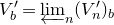$V^{\prime}_b = \varprojlim_n (V^{\prime}_n)_b$ . Moreover, a closed subspace of a space of compact type is also of compact type and so is the relevant quotient; $C_{c,K}$ is closed under countable direct sums.

Nuclear Banach spaces are finite dimensional. Nuclear Fréchet spaces are reflexive. Moreover, a subspace of a nuclear space is nuclear and if this subspace is closed the relevant quotient is nuclear. A countable inductive limit of nuclear spaces is nuclear (see [Reference Perez-Garcia and SchikhofPS10, Theorem 8.5.7]). By [Reference Perez-Garcia and SchikhofPS10, Theorem 8.5.7], projective limits of nuclear spaces are nuclear. Any compact projective or inductive limitFootnote ¹¹ of locally convex K-vector spaces is nuclear. A Fréchet space is the strong dual of a space of compact type if and only if it is nuclear.

The following lemma is essential for us.

It is an algebraic isomorphism and it is continuous. Hence, we just need to check that it is open. Thus, let $U_\lambda$ be an open lattice in $\mathrm{Ker}\,\lambda$ and let $V_0$ be an open lattice in V. We need to show that $U_\lambda+V_0$ is open in W and it is enough to do it for open sub-lattices of $U_\lambda$ and $V_0$ .

Any neighborhood of 0 in $\mathrm{Ker}\,\lambda$ contains an open of the form $U\cap(\mathrm{Ker}\,\lambda)$ , where U is an open lattice in W. Hence, we can assume $U_\lambda$ to be of this form. By construction, we have an exact sequence $0\to U_\lambda\to U\to\lambda(U)\to 0$ .

Now, U contains $p^NV_0$ for N big enough, since it is a lattice. Then $U_\lambda+p^NV_0$ is the inverse image of $p^N\lambda(V_0)$ in U by $\lambda$ , hence it is open as $\lambda$ is continuous and $p^N\lambda(V_0)$ is open in K. We proved what we wanted, up to replacing $V_0$ by its sub-lattice $p^NV_0$ .

The second claim follows immediately from the first.

such that $V,V_1$ are of finite rank over K and the map $f_{W'}$ is compact, then the map $f_W$ is compact as well.

Take an open lattice $L_{W'}$ in W’ such that $f_{W'}(L_{W'})$ is compactoid. Let $L_W$ be the preimage of $L_{W'}$ in W. Choose a section $s: W_1'\to W_1$ of the projection $\pi: W_1\to W_1'$ and consider the continuous map

\begin{align*} g: W\to V_1,\quad g(w):=f_W(w)-s\pi(f_W(w)). \end{align*}

Take a compact lattice $L_{V_1}$ in $V_1$ , its preimage (via g) in W, and then change $L_W$ to its intersection with that preimage.

Now, we see that $f_W(L_W)$ is compactoid: we have

\begin{align*} f_W(L_W)\subset g(L_W)+sf_{W'}(L_{W'}) \end{align*}

and both $g(L_W)$ and $sf_{W'}(L_{W'})$ are compactoid in $W_1$ . This concludes the proof of our lemma.

Let $C_{nF,K}$ denote the full subcategory of $C_K$ consisting of nuclear Fréchet spaces. The functor

\begin{align*} C_{c,K}\to C_{nF,K},\quad V\mapsto V^{\prime}_b, \end{align*}

is an anti-equivalence of categories. For any two $V,W\in C_{c,K}$ the natural linear map ${\mathscr{L}}_b(V,W)\to {\mathscr{L}}_b(W^{\prime}_b, V^{\prime}_b)$ is a topological isomorphism.

2.2.1 Basic properties of condensed sets.

Let Cond denote the category of condensed sets, i.e. sheaves of sets on the site of pro-finite sets with coverings given by finite families of jointly surjective mapsFootnote ¹² or, equivalently, on the pro-étale site $*_{{{\mathrm{pro\acute{e}t}}}}$ of a geometric point. We define similarly condensed groups, rings, etc.

We denote by CondAb the category of condensed abelian groups. It is an abelian category [Reference Clausen and ScholzeCS19, Theorem 2.2]. It has all limits and colimits. Arbitrary products, arbitrary direct sums, and filtered colimits are exact. It is generated by compact projective objects. For a condensed commutative ring A, we write $\mathrm{Mod}^\mathrm{cond}_A$ for the category of A-modules in $\mathrm{CondAb} $ and $\underline{{{\rm Hom}} }_A(-,-) $ for its internal ${{\rm Hom}} $ (in the case $A = \mathbf{Z}$ , we often omit the subscript $\mathbf{Z}$ ).

For a condensed set X, we think of $X(*)$ as the underlying set of X and about X(S) as the continuous maps from S to X. A quasi-separatedFootnote ¹³ condensed set X is trivial as soon as $X(*)$ is trivial (a fact that is false for a general X, see [Reference Clausen and ScholzeCS20, Lecture I]).

Let Top denote the category of T1 topological spaces.Footnote ¹⁴ We have a functor

\begin{align*}(\underline{\phantom{x}}): \mathrm{Top} \to \mathrm{Cond},\quad T \mapsto \underline{T}={\mathscr{C}}(S, T),\end{align*}

where ${\mathscr{C}}(S, T)$ denotes the set of continuous functions from S to T. Condensed sets that come from topological spaces we call classical. We quote the following.

1. (i) has a left adjoint $X\mapsto X(*)_\mathrm{top}$ sending any condensed set X to the set $X(*) $ equipped with the quotient topology arising from the map

   \begin{align*}\coprod\nolimits_{S,a\in X(S)}S \overset{a}{\to} X(*);\end{align*}

2. (ii) restricted to compactly generated topological spaces is fully faithful;

3. (iii) induces an equivalence between the category of compact Hausdorff spaces and quasi-compact quasi-separated (qcqs) condensed sets;

4. (iv) induces a fully faithful functor from the category of compactly generated weak HausdorffFootnote ¹⁵ spaces, to quasi-separated condensed sets; the category of quasi-separated condensed sets is equivalent to the category of ind-compact Hausdorff spaces ‘ $\operatorname{colim} _n$ ’ $X_n$ , where all transition maps are closed immersions; if $\{X_n\}_{n\in\mathbf{N}}$ is a ind-system of compact Hausdorff spaces with closed immersions and $X = \operatorname{colim} _n X_n$ as topological spaces, then the canonical map

   \begin{align*}\operatorname{colim} _n \underline{X_n}\to\underline{X}\end{align*}
   is an isomorphism of condensed sets; in particular, $\operatorname{colim} _n \underline{X_n}$ is classical, i.e. it comes from a topological space.

2.2.2 Solid modules.

We briefly review basic facts concerning solid modules.

Analytic rings. We start with analytic rings.

1. (i) (Clausen and Scholze [Reference Clausen and ScholzeCS19, Theorem 5.8].) The analytic ring $\mathbf{Z}_{\Box}=(\mathbf{Z},{\mathscr{M}}_{\mathbf{Z}})$ is defined as the ring $\mathbf{Z}$ equipped with the functor of measures ${\mathscr{M}}_{\mathbf{Z}}$ sending an extremally disconnected set $S=\lim_i S_i$ , where each $S_i$ is a finite set, to the condensed abelian group $\mathbf{Z}_{\Box}:=\lim_i\mathbf{Z}[S_i]$ .

2. (ii) (Clausen and Scholze [Reference Clausen and ScholzeCS19, Proposition 7.9].) Let K be a finite extension of $\mathbf{Q}_p$ . There is an analytic structure on the condensed rings ${\mathscr O}_K$ and K given by sending an extremally disconnected set $S=\lim_i S_i$ , where each $S_i$ is finite, to

   \begin{align*}{\mathscr O}_{K,\Box}[S]:=\lim_i{\mathscr O}_K[S_i],\quad K_{\Box}[S]:=K\otimes_{{\mathscr O}_K}{\mathscr O}_{K,\Box}[S].\end{align*}
   The first analytic ring structure is induced from the analytic ring structure of $\mathbf{Z}_{\Box}$ by base change to ${\mathscr O}_K$ .

Solid modules. Now we pass to solid modules.

1. (i) The full subcategory of solid A-modules

   (2.13) \begin{equation} \mathrm{Mod}^\mathrm{solid}_{A}\subset \mathrm{Mod}^\mathrm{cond}_A \end{equation}
   consists of all A-modules M such that, for all extremally disconnected sets S, the maps
   \begin{align*} {{\rm Hom}} _A({\mathscr{M}}_A[S],M)\to {{\rm Hom}} _A(A[S],M) \end{align*}
   are isomorphisms. It is an abelian subcategory, stable under all limits, colimits, and extensions. The inclusion (2.13) admits a left adjoint
   (2.14) \begin{equation} \mathrm{Mod}^\mathrm{cond}_A\to \mathrm{Mod}^\mathrm{solid}_{A} : \quad M \mapsto M \otimes_A (A,{\mathscr{M}}_A), \end{equation}
   which preserves all colimits and is symmetric monoidal.

2. (ii) The functor

   (2.15) \begin{equation}{\mathscr{D}}(\mathrm{Mod}^\mathrm{solid}_{A})\to {\mathscr{D}}(\mathrm{Mod}^\mathrm{cond}_{A})\end{equation}
   is fully faithful. Its essential image is stable under all limits and colimits. It is given by complexes $M \in {\mathscr{D}}(\mathrm{Mod}^\mathrm{cond}_{A}) $ such that the map
   \begin{align*}{\mathrm R} {{\rm Hom}} _A({\mathscr{M}}_A[S],M)\to {\mathrm R}{{\rm Hom}} _A(A[S],M)\end{align*}
   is a quasi-isomorphism for all extremally disconnected sets S.

   A complex $M \in {\mathscr{D}}(\mathrm{Mod}^\mathrm{cond}_A)$ is in ${\mathscr{D}}(\mathrm{Mod}^\mathrm{solid}_{A})$ if and only if $H^i(M)$ is in $\mathrm{Mod}^\mathrm{solid}_{A}$ , for all i. The functor (2.15) admits a left adjoint

   (2.16) \begin{equation}{\mathscr{D}}(\mathrm{Mod}^\mathrm{cond}_A) \to {\mathscr{D}}(\mathrm{Mod}^\mathrm{solid}_{A}) : M\mapsto M\otimes^\mathrm{L}_A(A,{\mathscr{M}}_A),\end{equation}
   which is the left derived functor of (2.14). It is symmetric monoidal.

3. (iii) For $M, N \in {\mathscr{D}}(\mathrm{Mod}^\mathrm{solid}_{A})$ , we have the derived internal Hom

   \begin{align*}{\mathrm R}\underline{{{\rm Hom}} }_{A}(M,N)\in{\mathscr{D}}(\mathrm{Mod}^\mathrm{ solid}_{A}).\end{align*}
   The natural map ${\mathrm R}\underline{{{\rm Hom}} }_{(A,{\mathscr{M}}_A)}(M,N) \to {\mathrm R}\underline{{{\rm Hom}} }_A(M,N)$ is a quasi-isomorphism.

2.2.3 Locally convex and condensed vector spaces.

Consider the functor

\begin{align*}\mathrm{CD}:=(\underline{\phantom{x}}): \quad C^\mathrm{Hcg}_K\to \mathrm{Mod}^\mathrm{cond}_{{K}}, \quad V\mapsto \underline{V}.\end{align*}

We denote in the same way its extension to the category of complexes. By Lemma 2.18, the functor CD preserves (strict) quasi-isomorphisms of complexes of Fréchet spaces or spaces of compact type and if V is such a complex, then

\begin{align*}\mathrm{CD}(\widetilde{H}^i(V))\simeq H^i(\mathrm{CD}(V)).\end{align*}

Assume first that both V and W are Fréchet. In that case we have the following argument of Bosco [Reference BoscoBos21, Lemma 1.A.33]: since g(S) is compact in W, by [Reference TrevesTre67, Lemma 45.1], it is the image f(H) of a compact subset H of V. We conclude by recalling that the extremally disconnected sets are the projective objects of the category of compact Hausdorff topological spaces.

Assume now that both V and W are of compact type. Since g(S) is compact in W, if we write $W=\operatorname{colim} _n W_n$ , for an ind-system $\{W_n\}_{n\in\mathbf{N}}$ of Banach spaces over K with compact injective transition maps, then $g(S)\subset W_m$ , for some $m\in\mathbf{N}$ (see [Reference SchneiderSch02, Lemma 16.9]). By [Reference Rodrigues Jacinto and Rodriguez CamargoRR21, Lemma 3.39], we have a commutative diagram of solid arrows

for a K-Banach space $V_m$ . As above, it follows that the dashed arrow exists, which concludes our proof of the lemma.

2.2.4 Solid Fréchet spaces and solid spaces of compact type.

We define solid Fréchet spaces and solid spaces of compact type as the images in the category of solid K-vector spaces of their classical analogs. See [Reference Rodrigues Jacinto and Rodriguez CamargoRR21, Chapter 3] for alternative definitions.

(i) Solid Fréchet spaces. A solid Banach space is a solid K-vector space of the form $\underline{V}$ , for a classical Banach space V. A solid Fréchet space is a solid K-vector space of the form $\underline{V}$ , for a classical Fréchet space V. It is called nuclear if V is nuclear. The functor $(\underline{\quad})$ identifies the categories of classical and solid Fréchet spaces (identifying also exact sequences by Lemma 2.18). If this does not cause confusion we use the term ‘Fréchet spaces’ for elements of both of these categories.

Warning. The definition of nuclear used here is stronger than the definition of nuclear in the solid formalism. To distinguish, we call the latter ‘solid nuclear’.

Let V be a solid Fréchet space written as a limit $V=\lim_n V_n$ of Banach spaces $V_n$ with dense transition maps. Then we have the following.

1. (i) (Topological Mittag–Leffler [Reference Rodrigues Jacinto and Rodriguez CamargoRR21, Lemma 3.27].) Then

   \begin{align*}{\mathrm R}^j\lim_n V_n=0,\quad j\geqslant 1.\end{align*}
   In particular, $V\simeq {\mathrm R}\underline{{{\rm Hom}} }_K(V^*,K)$ .

2. (ii) If W is a Banach space, then $\underline{{{\rm Hom}} }_K(V,W)=\operatorname{colim} _n\underline{{{\rm Hom}} }_K(V_n,W)$ (see [Reference Rodrigues Jacinto and Rodriguez CamargoRR21, Lemma 3.3]).

3. (ii) Solid spaces of compact type. A solid space of compact type is a solid K-vector space of the form $\underline{V}$ , for a classical space of compact type V. The functor $(\underline{\quad})$ identifies the categories of classical and solid spaces of compact type (identifying also exact sequences by Lemma 2.18). If this does no confusion we use the term ‘spaces of compact type’ for elements of both of these categories.

The following two lemmas are needed later.

Lemma 2.19. Let $V\in C_K$ be of compact type. Write it as $V\simeq \operatorname{colim} _n V_n$ with $V_n$ , $n\in\mathbf{N}$ , Hausdorff and injective compact transition maps. Then we have a canonical isomorphism of condensed K-modules

\begin{align*} \operatorname{colim} _n \underline{V_n}\stackrel{\sim}{\to} \underline{V}. \end{align*}

In particular, the condensed K-module $ \operatorname{colim} _n \underline{V_n}$ is classical.

Proof. We start with an exact sequence of solid Fréchet spaces over K

\begin{align*} 0\to \underline{V}_1\to \underline{V}_2\to \underline{V}_3\to 0. \end{align*}

We need to show that the sequence of classical Fréchet spaces

(2.21) \begin{equation} 0\to {V}_1\stackrel{f_1}{\to} {V}_2\to V_3\to 0 \end{equation}

is strictly exact. But the sequence

(2.22) \begin{equation} 0\to \underline{V}_1(*)_\mathrm{top}\to \underline{V}_2(*)_\mathrm{top}\to \underline{V}_3(*)_\mathrm{top}\to 0 \end{equation}

maps, via topological isomorphisms $\underline{V}_i(*)_\mathrm{top}\stackrel{\sim}{\to} V_i$ (since $V_i$ is compactly generated), to the sequence (2.21). Since $\underline{V_3}$ is quasi-separated, the map $f_1$ is a closed immersion. In particular, we have a strict exact sequence of Fréchet spaces

\begin{align*} 0\to {V}_1\stackrel{f_1}{\to} {V}_2\to V'_3\to 0 \end{align*}

and a continuous injection $f_2: V'_3\to V_3$ . We need to prove that the map $f_2$ is a topological isomorphism. Since $f_2$ is a map between two Fréchet spaces, by the open mapping theorem, it suffices to show that $f_2$ is an algebraic isomorphism. But, by Lemma 2.18, we have the exact sequence

\begin{align*} 0\to \underline{V}_1\to \underline{V}_2\to \underline{V}'_3\to 0.\end{align*}

Hence, the canonical map $\underline{f}_2: \underline{V}'_3 \to \underline{V}_3$ is an isomorphism, which yields that so is the map $f_3$ (by the faithfullness of the $(\underline{\phantom{x}})$ functor.

The argument for spaces of compact type is similar (the open mapping theorem is valid for LB spaces).

2.2.5 Solid tensor product.

We list properties of the solid tensor product that we often use.

1. (i) [Reference BoscoBos21, Proposition A.68]. Let V, W be Fréchet spaces over K. Then we have a natural isomorphism of solid K-vector spaces

   \begin{align*} \underline{V}\otimes_{K}^{\Box}\underline{W}\stackrel{\sim}{\to}\underline{V\widehat{\otimes}_KW}, \end{align*}
   where $V\widehat{\otimes}_KW$ denotes the projective tensor product in the category $C_K$ .

2. (ii) [Reference BoscoBos21, Corollary A.65]. Any Fréchet space over K is acyclic for the tensor product $\otimes^{\Box}_{K}$ . That is, if V is a Fréchet space over K then $(-)\otimes^{\mathrm{L}\Box}_KV\simeq (-)\otimes^{\Box}_KV$ .

3. (iii) [Reference BoscoBos21, Corollary A.67].

   1. (a) Let $\{V_n\}_{n\in\mathbf{N}}$ be a pro-system of solid nuclear K-vector spaces and let W be a Fréchet vector space over K. Then we have an isomorphism

      \begin{align*} \lim_n (V_n\otimes_{K}^{\Box}W)\stackrel{\sim}{\leftarrow}(\lim_n V_n)\otimes_{K}^{\Box}W. \end{align*}

   2. (b) Let $\{V_n\}_{n\in\mathbf{N}}$ be a pro-system in ${\mathscr{D}}(K_{\Box})$ of complexes of solid nuclear K-vector spaces. Let W be a complex of K-Fréchet spaces. Then we have a quasi-isomorphism

      \begin{align*} {\mathrm R} \lim_n (V_n\otimes_{K}^{\mathrm{L}\Box}W)\stackrel{\sim}{\leftarrow}({\mathrm R}\lim_n V_n)\otimes_{K}^{\mathrm{L}\Box}W. \end{align*}

The above properties also hold if we replace K with $\breve{F}$ (with the same references).

3.1.1 Condensed Galois cohomology.

Let G be a condensed group. A condense G-module is a condensed abelian group endowed with a $\mathbf{Z}[G]$ -module structure. The condensed group cohomology of G with values in a condense G-module V is defined as

\begin{align*}{\mathrm R}\Gamma(G,V):={\mathrm R}\underline{{{\rm Hom}} }_{\mathbf{Z}[G]}(\mathbf{Z},V)\in{\mathscr{D}}(\mathrm{CondAb}).\end{align*}

We list the following properties of ${\mathrm R}\Gamma(G,-)$ .

1. (i) [Reference BoscoBos21, Proposition B.2]. Let G be a profinite group and let V be a G-module in solid abelian groups. Then we have the following.

   1. (a) The complex ${\mathrm R}\Gamma({G},V)$ is quasi-isomorphic to the complex of solid abelian groups

      (3.2) \begin{equation}V\to \underline{{{\rm Hom}} }(\mathbf{Z}[{G}^1],V)\to \underline{{{\rm Hom}} }(\mathbf{Z}[{G}^2],V)\to \underline{{{\rm Hom}} }(\mathbf{Z}[{G}^3],V)\cdots.\end{equation}

   2. (b) If $V=\underline{V_\mathrm{top}}$ , with $V_\mathrm{top}$ a T1 topological G-module over $\mathbf{Z}$ , then, for all $i\geqslant 0$ , we have a natural isomorphism in ${\mathscr{D}}(\mathrm{Ab})$ (the second cohomology is the continuous group cohomology computed via the pro-étale site of a point):

      \begin{align*}{\mathrm R}\Gamma({G},V)(*)\simeq {\mathrm R}\Gamma({G},V_\mathrm{top}).\end{align*}

2. (ii) [Reference BoscoBos21, Proposition B.3]. For $n\in\mathbf{N}$ , let $\Gamma:=\mathbf{Z}_p^n$ , and let $\gamma_1,\ldots,\gamma_n$ denote the generators of $\Gamma$ . Let V be a $\Gamma$ -module in $\mathrm{Mod}^\mathrm{solid}_{\mathbf{Z}_p}$ . Then we have a quasi-isomorphism

   \begin{align*}{\mathrm R}\Gamma(\Gamma,V)\simeq \mathrm{Kos}_{\gamma}(V):=\mathrm{Kos}_V(\gamma_1-1,\ldots,\gamma_n-1),\end{align*}
   the Koszul complex of V with respect to the elements $\gamma_1-1,\ldots,\gamma_n-1$ .

3. (iii) [Reference Rodrigues Jacinto and Rodriguez CamargoRR21, Lemma 5.2]. Let G be a profinite group. There is a solid projective resolution of the trivial representation

   \begin{align*}\cdots \to K_{\Box}[{G}^{n+1}]\to K_{\Box}[{G}^{n}]\to \cdots\to K_{\Box}[{G}^{1}]\to K\to 0.\end{align*}
   In particular, if V is a G-module in solid modules over K, one has that
   \begin{align*}{\mathrm R} \underline{{{\rm Hom}} }_{K_{\Box}[G]}(K,V)\simeq {\mathrm R}\Gamma({G},V).\end{align*}

1. (1) we have a quasi-isomorphism and isomorphisms

   \begin{align*} \mathrm{CD}({\mathrm R}\Gamma({G},V))\simeq {\mathrm R}\Gamma({G},\underline{V}),\quad \mathrm{CD}(\widetilde{H}^i({G},V))\simeq H^i({G},\underline{V}),\ i\geqslant 0;\end{align*}

2. (2) we have a quasi-isomorphismFootnote ¹⁶ in ${\mathscr{D}}(C_{\mathbf{Q}_p})$

   \begin{align*} {\mathrm R}\Gamma({G},\underline{V})(*)_\mathrm{top}\simeq {\mathrm R}\Gamma({G},V).\end{align*}

Proof. For claim (1) we compute

\begin{align*} {\mathrm R}\Gamma({G},V)& \simeq C(G,V),\quad n\mapsto {\mathscr{C}}(G^{n-1},V);\\ \mathrm{CD}({\mathrm R}\Gamma({G},V))(S): n & \mapsto {\mathscr{C}}(S,{\mathscr{C}}(G^{n-1},V))\simeq {\mathscr{C}}(S\times G^{n-1},V),\end{align*}

where S is a profinite set and ${\mathscr{C}}(-,-)$ denotes the space of continuous maps equipped with compact open topology (note that $ {\mathscr{C}}(S\times G^{n-1},V)$ , since $S\times G^{n-1}$ is compact, is a $\mathbf{Q}_p$ -Banach space). We also have

\begin{align*} {\mathrm R}\Gamma({G},\underline{V}): n & \mapsto \underline{{{\rm Hom}} }(\mathbf{Z}[{G}^{n-1}],\underline{V});\\ \underline{{{\rm Hom}} }(\mathbf{Z}[{G}^{n-1}],\underline{V})(S) & ={{{\rm Hom}} }(\mathbf{Z}[{S}]\otimes \mathbf{Z}[{G}^{n-1}],\underline{V})\simeq {{{\rm Hom}} }(\mathbf{Z}[{S\times G^{n-1}}],\underline{V}).\end{align*}

Since ${{{\rm Hom}} }(\mathbf{Z}[{S\times G^{n-1}}],\underline{V})\simeq {\mathscr{C}}(S\times G^{n-1},{V})$ , we get claim (1) of the lemma.

Claim (2) follows from the fact that the complex of continuous cochains representing $ {\mathrm R}\Gamma({G},V)$ is a complex of Banach spaces and [Reference Rodrigues Jacinto and Rodriguez CamargoRR21, Proposition 3.5].

3.1.2 Poitou–Tate duality.

Let K be a finite extension of $\mathbf{Q}_p$ and let V be a continuous, finite rank $\mathbf{Q}_p$ -representation of ${\mathscr{G}}_K$ . Recall that the Galois pairing

\begin{align*}H^i({\mathscr{G}}_K,V)\otimes^{\Box}_{\mathbf{Q}_p} H^{2-i}({\mathscr{G}}_K,V^*(1))\stackrel{\cup}{\to} H^2({\mathscr{G}}_K,\mathbf{Q}_p(1))\xrightarrow[\sim]{\mathrm{Tr}_{K}}\mathbf{Q}_p\end{align*}

is a perfect pairing (by Poitou–Tate duality). Hence, for $i\in\mathbf{N}$ , $H^i({\mathscr{G}}_K,V)$ and $H^{2-i}({\mathscr{G}}_K,V^*(1))$ are natural duals (via the above pairing). In particular, we have

\begin{align*}H^0({\mathscr{G}}_K,\mathbf{Q}_p(j)) & \simeq \begin{cases} \mathbf{Q}_p&{\text{if $j=0$,}}\\0 &{\text{otherwise;}}\end{cases}\quad H^2({\mathscr{G}}_K,\mathbf{Q}_p(j))\simeq \begin{cases} \mathbf{Q}_p&{\text{if $j=1$,}}\\0 &{\text{otherwise.}}\end{cases}\end{align*}

3.2.1 Notation.

If $n\geqslant 1$ , let $F_n=\mathbf{Q}_p({\boldsymbol\mu}_{p^n})$ and let $F_\infty:=\bigcup_nF_n$ be the cyclotomic extension of $\mathbf{Q}_p$ . Let $\chi:\mathscr{G}_{\mathbf{Q}_p}\to\mathbf{Z}_p^{\boldsymbol *}$ be the cyclotomic character. Then $\chi$ factors through $\Gamma:=\mathrm{Gal}(F_\infty/\mathbf{Q}_p)$ and induces an isomorphism $\chi:\Gamma\overset{\sim}{\to}\mathbf{Z}_p^{\boldsymbol *}$ .

If $\Delta$ is the torsion subgroup of $\Gamma$ , then $\chi^{|\Delta|}$ takes values in $1+p\mathbf{Z}_p$ (respectively, $1+8\mathbf{Z}_2$ ) if $p\neq 2$ (respectively, $p=2$ ). Let $\tau:\mathscr{G}_{\mathbf{Q}_p}\to\mathbf{Z}_p$ be defined by

\begin{align*}\tau=\begin{cases}\dfrac{1}{p\,|\Delta|}\log\chi^{|\Delta|}&{\text{if} p\neq 2,}\\[10pt]\dfrac{1}{4\,|\Delta|}\log \chi^{|\Delta|}&{\text{if} p= 2.}\end{cases}\quad{\text{i.e. }}\tau=\frac{1}{p^{c(p)}}\log\chi,\ \mathrm{with}\ {c(p)}=\begin{cases} 1 &{\text{if} p\neq 2,}\\ 2 &{\text{if} p= 2.}\end{cases}\end{align*}

Let $F_\infty':=F_\infty^\Delta$ be the cylotomic $\mathbf{Z}_p$ -extension of $\mathbf{Q}_p$ . Then $\tau$ factors through $\Gamma':=\mathrm{Gal}(F_\infty'/\mathbf{Q}_p)$ and induces an isomorphism $\tau:\Gamma'\overset{\sim}{\to}\mathbf{Z}_p$ .

Let K be a finite extension of $\mathbf{Q}_p$ . If $n\in\mathbf{N}$ , let $K_n=K({\boldsymbol\mu}_{p^n})$ and let $K_\infty:=\bigcup_n K_n$ be the cyclotomic extension of K. Let $\Gamma_K:=\mathrm{Gal}(K_\infty/K)$ ; then $\chi$ induces an isomorphism from $\Gamma_K$ to an open subgroup of $\mathbf{Z}_p^{\boldsymbol *}$ . Let $\Delta_K$ be the torsion subgroup of $\Gamma_K$ , let $K'_\infty:=K_\infty^{\Delta_K}$ be the cylotomic $\mathbf{Z}_p$ -extension of K. Then $\Gamma_K':=\mathrm{Gal}(K_\infty'/K)=\Gamma_K/\Delta_K$ and $\tau$ induces an isomorphism $\tau:\Gamma_K'\overset{\sim}{\to}p^{n(K)}\mathbf{Z}_p$ for some $n(K) \in\mathbf{N}$ .

Let $\gamma_K\in\Gamma'_K$ be the element verifying $\tau(\gamma_K)=p^{n(K)}$ . Then $\gamma_K$ has a unique lifting in $\Gamma_K$ whose image by $\chi$ belongs to $1+p^{n(K)+c(p)}\mathbf{Z}_p$ ; we denote this lifting also by $\gamma_K$ . Then $\Gamma_K=\gamma_K^{\mathbf{Z}_p}\times\Delta_K$ .

Let $L=K({\boldsymbol\mu}_{p^{c(p)}})$ . Then $\mathrm{Gal}(L/K)=\Delta_K$ and $\Gamma_L=\gamma_K^{\mathbf{Z}_p}$ .

Let $\varepsilon\in\mathscr{O}_{K_\infty}^\flat$ , with $\varepsilon^\sharp=1$ and $(\varepsilon^{1/p})^\sharp\neq 1$ (where $x^\sharp=\theta([x])$ as usual), and let $t:=\log[\varepsilon]$ be Fontaine’s $2\pi i$ , viewed as a regular function of the Fargues–Fontaine

\begin{align*}Y_{\mathrm{FF},K_\infty}:=\mathrm{Spa}(W(\mathscr{O}_{K_\infty}^\flat))\boldsymbol{\backslash}\{p=0,[\varepsilon-1]=0\}.\end{align*}

It satisfies $\varphi(t)=pt$ and $\sigma(t)=\chi(\sigma)t$ if $\sigma\in\Gamma_K$ , and its divisor is the orbit under $\varphi$ of the point $\infty$ defined by $\mathrm{Ker}(\theta:W(\mathscr{O}_{K_\infty}^\flat{\kern-1pt})\to \mathscr{O}_{K_\infty}{\kern-1pt})$ .

For $0\lt u\leqslant v\in v(K_\infty^\flat)$ , let

\begin{align*}\mathbf{B}_{K_\infty}^{[u,v]}:=\bigg(W(\mathscr{O}_{K_\infty}^\flat)\bigg[\frac{p}{[\alpha]},\frac{[\beta]}{p}\bigg]^{\wedge_p}\bigg)\bigg[\frac{1}{p}\bigg],\quad v(\alpha)=\frac{1}{v},\ v(\beta)=\frac{1}{u}.\end{align*}

It is a Banach space over $\mathbf{Q}_p$ . Let $U^{[u,v]}$ be the corresponding open set of $Y_{\mathrm{FF},K_\infty}$ -1pt. Take $u=({p-1})/{p}$ , $v=p-1$ if $p\neq 2$ , and $u=\frac{2}{3}$ , $v=\frac{4}{3}$ if $p=2$ . Then $\theta$ induces an identification $\mathbf{B}^{[u,v]}_{K_\infty}/t=\widehat K_\infty$ and t is a unit inFootnote ¹⁷ $\mathbf{B}^{[u,v/p]}_{K_\infty}$ .

3.2.2 Galois cohomology.

The Frobenius $\varphi$ induces an isomorphism $\mathbf{B}_{K_\infty}^{[u,v]}\overset{\sim}{\to} \mathbf{B}_{K_\infty}^{[u/p,v/p]}$ , hence also a morphism $\mathbf{B}_{K_\infty}^{[u,v]}\overset{\sim}{\to} \mathbf{B}_{K_\infty}^{[u,v/p]}$ . For $j\in\mathbf{Z}$ , standard $(\varphi,\Gamma)$ -modules techniques (see Remark 3.6) yield quasi-isomorphisms:

(3.5) \begin{equation}\begin{aligned}\alpha_j: \mathrm{Kos}_{\varphi,\gamma}(\mathbf{B}^{[u,v]}_{K_\infty}(j))&\simeq \mathrm{R}\Gamma({\mathscr{G}}_L,\mathbf{Q}_p(j)),\\\alpha_j:\mathrm{Kos}_{\varphi,\gamma}(\mathbf{B}^{[u,v]}_{K_\infty}(j))^{\Delta_K}&\simeq \mathrm{R}\Gamma({\mathscr{G}}_K,\mathbf{Q}_p(j)),\end{aligned}\end{equation}

where the $(\varphi,\gamma)$ -Koszul complexes (of Banach spaces over $\mathbf{Q}_p$ ) are defined by

and the complex $\mathrm{Kos}_{\varphi,\gamma}(\mathbf{B}^{[u,v]}_{K_\infty}(j))^{\Delta_K}$ is obtained by taking fixed points under $\Delta_K$ of each of the terms of the complex.

Set $[\Delta_K]:=\sum_{\sigma\in\Delta_K}\sigma$ . The following commutative diagram allows us to deduce results for K from results for L, i.e. we can often assume that $\Delta_K=1$ in the proofs.

Applying $\mathrm{Res}_{p^{-n}\mathbf{Z}_p}$ to each of the terms of the above complex produces a quasi-isomorphic complex with rings related to $K_n$ instead of $K_\infty$ , which is closer to the complexes used in the theory of $(\varphi,\Gamma)$ -modules, like in Herr’s thesis [Reference HerrHer98] or in [Reference Cherbonnier and ColmezCC99]. Going from these rings to the usual rings uses the standard techniques of $(\varphi,\Gamma)$ -modules, i.e. normalized trace $\mathrm{Res}_{p^{-n}\mathbf{Z}_p}$ , bijectivity of $\gamma_K-1$ on $(\mathbf{B}^{[u/p^n,v/p^n]}_{K}(j))^{\psi=0}$ , etc., as in [Reference Colmez and NiziołCN17, §§ 4.4–4.6].

3.2.3 Examples.

Denote by

(3.7) \begin{equation}h^i_K:Z^i(\mathrm{Kos}_{\varphi,\gamma}(\mathbf{B}^{[u,v]}_{K_\infty}(j))^{\Delta_K})\to H^i({\mathscr{G}}_K,\mathbf{Q}_p(j))\end{equation}

the map induced by quasi-isomorphism (3.5); it factorizes as

\begin{align*}h^i_K:Z^i(\mathrm{Kos}_{\varphi,\gamma}(\mathbf{B}^{[u,v]}_{K_\infty}(j))^{\Delta_K})\to H^i(\mathrm{Kos}_{\varphi,\gamma}(\mathbf{B}^{[u,v]}_{K_\infty}(j))^{\Delta_K})\simeq H^i({\mathscr{G}}_K,\mathbf{Q}_p(j)).\end{align*}

If $(a,b)\in Z^1(\mathrm{Kos}_{\varphi,\gamma}(\mathbf{B}_{K_\infty}^{[u,v]}(j))^{\Delta_K})$ and $u\in\mathbf{B}_{\overline K}^{[u,v]}(j)$ satisfy $(\varphi-1)u=a$ , then

(3.8) \begin{equation}h^1_K(a,b)=\mathrm{cl}\!\left(\sigma\mapsto\frac{\sigma-1}{\gamma_K-1}b-(\sigma-1)u\!\right)\!.\end{equation}

(In this expression, $\sigma$ acts through its image in $\Gamma'_K$ on b, and we think of $({\sigma-1})/({\gamma_K-1})$ as an element of $\mathbf{Z}_p[[\Gamma'_K]]$ ; the expression between parenthesis is a 1-cocycle on ${\mathscr{G}}_K$ with values in $\mathbf{Q}_p(j)$ , and cl denotes its image in $H^1({\mathscr{G}}_K,\mathbf{Q}_p(j))$ .)

The case $j=0$ . We can apply the formula (3.8) to $j=0$ and cocycle (1,0). Then the corresponding ${\mathscr{G}}_K$ -cocycle factors through $\mathrm{Gal}(\overline{\mathbf{F}}_p/k_K)$ since the solution of $(\varphi-1)u=1$ belongs to $W(\overline{\mathbf{F}}_p)$ , and sends the relative Frobenius to $f:=f(K/\mathbf{Q}_p)$ (because $(\sigma-1)u$ is equal to $(\varphi^f-1)u=f$ since $\varphi(u)=u+1$ ). Since the relative Frobenius corresponds to a uniformizer of $K^{\boldsymbol *}$ , it follows that the element $\lambda$ of $\mathrm{Hom}(K^{\boldsymbol *},\mathbf{Q}_p)$ which corresponds to $h^1_K(1,0)$ is $f(K/\mathbf{Q}_p) v_K=v_p\circ\mathrm{N}_{K/\mathbf{Q}_p}$ (where $v_K$ is the valuation on K with image $\mathbf{Z}$ ).

Starting with $(0,p^{n(K)+c(p)})$ , formula (3.8) with $u=0$ yields a group morphism $\mathscr{G}_K\to\mathbf{Z}_p$ which factors through $\Gamma'_K$ and has value $\log\chi(\gamma_K)$ at $\gamma_K$ ; it follows that this morphism is $\log\chi$ .

The case $j=1$ . Let $n=n(K)+c(p)$ . We have $(\varphi-1)\tfrac{1}{\pi}\in (\mathbf{B}_{\mathbf{Q}_p}^{(0,v]})^{\psi=0}$ and there exists $a\in(\mathbf{B}_{\mathbf{Q}_p}^{(0,v/p^n]})^{\psi=0}\otimes {d\pi}/({1+\pi})$ such that $(\gamma_K-1)a=((\varphi-1)\tfrac{1}{\pi})\otimes{d\pi}/({1+\pi})$ . Then,

\begin{align*} \left(\varphi^{-n}(a),\varphi^{-n}\left(\frac{1}{\pi}\otimes \frac{d\pi}{1+\pi}\right)\!\right)\in Z^1(\mathrm{Kos}_{\varphi,\gamma}(\mathbf{B}_{F_n}^{[u,v]}(1))) \end{align*}

and

\begin{align*} h^1_{F_n}\left(\varphi^{-n}(a),\varphi^{-n}\left(\frac{1}{\pi}\otimes\frac{d\pi}{1+\pi}\right)\!\right)=\mathrm{cl}(\zeta_{p^n}-1). \end{align*}

(This follows from point iii) of [Reference Cherbonnier and ColmezCC99, Proposition V.3.2], using the constructions leading to [Reference Cherbonnier and ColmezCC99, Theorem II.1.3] and the (obvious) fact that Coleman power series attached to $(\zeta_{p^n}-1)_{n\geqslant 1}$ is just T.)

3.2.4 Cup products.

We define compatible cup products ( $\alpha\in\mathbf{Q}_p$ )

\begin{align*} \cup_{\alpha} : \mathrm{Kos}_{\varphi,\gamma}(\mathbf{B}^{[u,v]}_{K_\infty}(j_1))^{\Delta_K} & \otimes^{\Box}_{\mathbf{Q}_p} \mathrm{Kos}_{\varphi,\gamma}(\mathbf{B}^{[u,v]}_{K_\infty}(j_2))^{\Delta_K}\to \mathrm{Kos}_{\varphi,\gamma}(\mathbf{B}^{[u,v]}_{K_\infty}(j_1+j_2))^{\Delta_K} \end{align*}

using (twice) the formulas from § 7.3.2.

Proof. This is easy to check for the pairing of 0- and 2-cocycles. For the pairing of two 1-cocycles, this amounts to checking that

(3.10) \begin{equation}h^1_K(a,b)\cup h^1_K(a',b')=h^2_K(b\otimes\gamma_K(a')-a\otimes\varphi(b')).\end{equation}

(For the product on the Koszul complexes, we used here (twice) the formulas from § 7.3.2 with $\alpha=1$ .) But equality (3.10) is standard and was checked by Herr and Benois in [Reference HerrHer98, Reference BenoisBen00].

3.3.1 The trace map.

We describe the trace isomorphism

\begin{align*}\mathrm{Tr}_K:H^2({\mathscr{G}}_K,\mathbf{Q}_p(1))\overset{\sim}{\to}\mathbf{Q}_p\end{align*}

in terms of $(\varphi,\Gamma)$ -modules (cf. [Reference HerrHer98, Reference BenoisBen00]). For this, we start with the description of $\mathrm{Tr}_K$ given by local class field theory. We have isomorphisms

\begin{align*}\mathrm{cl}:\mathrm{Hom}(K^{\boldsymbol *},\mathbf{Q}_p)\overset{\sim}{\to}H^1({\mathscr{G}}_K,\mathbf{Q}_p)\quad\mathrm{and}\quad\mathbf{Q}_p\widehat{\otimes} K^{\boldsymbol *}\overset{\sim}{\to}H^1({\mathscr{G}}_K,\mathbf{Q}_p(1))\end{align*}

and $\mathrm{Tr}_K$ is given by the formula

\begin{align*}\mathrm{Tr}_K(\mathrm{cl}(\tau)\cup \mathrm{cl}(\alpha))=\tau(\alpha)\quad{\text{if $\tau\in \mathrm{Hom}(K^{\boldsymbol *},\mathbf{Q}_p)$ and $\alpha\in K^{\boldsymbol *}$.}}\end{align*}

3.3.2 Trace map and residues.

Let $\pi:=[\varepsilon]-1\in\mathbf{B}_{F_\infty}^{[u,v]}$ . We have $\gamma(\pi)=(1+\pi)^{\chi(\gamma)}-1$ if $\gamma\in\Gamma$ , and we make $\varphi$ and $\Gamma$ act on ${d\pi}/({1+\pi})$ by $\varphi({d\pi}/({1+\pi}))={d\pi}/({1+\pi})$ and $\gamma({d\pi}/({1+\pi}))=\chi(\gamma)({d\pi}/({1+\pi}))$ , respectively (this allows us to identify $\Lambda(1)$ with $\Lambda\otimes({d\pi}/({1+\pi}))$ ). Then there exists a unique continuous linear map

\begin{align*}\mathrm{res}_\pi:\mathbf{B}_{F_\infty}^{[u,v]}\otimes \frac{d\pi}{1+\pi}\to\mathbf{Q}_p,\end{align*}

which commutes with $\varphi$ and $\Gamma$ (with trivial actions of $\varphi$ and $\Gamma$ on $\mathbf{Q}_p$ ), and sends $\sum_{k\in\mathbf{Z}}a_k\pi^k\,d\pi$ to $a_{-1}$ . (See [Reference ColmezCol10, Proposition IV.3.3] for the existence of $\mathrm{res}_\pi$ .)

Set

\begin{align*}\mathrm{Tr}_{K_\infty/F_\infty}:=\sum\nolimits_{\sigma\in G_{F_\infty}/G_{K_\infty}} \sigma\end{align*}

(well-defined on modules on which $\mathscr{G}_{K_\infty}$ acts trivially).

Proposition 3.11. We have

\begin{align*}\mathrm{Tr}_K\circ h^2_K=\frac{1}{|\Delta_K|}\,\mathrm{res}_\pi\circ\mathrm{Tr}_{K_\infty/F_\infty}\quad \mathrm{on}\\bigg(\mathbf{B}_{K_\infty}^{[u,v/p]}\otimes\frac{d\pi}{1+\pi}\bigg)^{\Delta_K}.\end{align*}

Moreover, we have the following commutative diagram.

Hence, $\mathrm{Tr}_L\circ h^2_L=|\Delta_K|\,\mathrm{Tr}_K\circ h^2_K$ on $(\mathbf{B}_{K_\infty}^{[u,v/p]})^{\Delta_K}$ . It follows that the result holds for K if and only if it holds for L, and we can assume that $\Delta_K=1$ , i.e. $K=K_n$ , with $n=n(K)+c(p)$ .

Let $\lambda=v_p\circ\mathrm{N}_{K/\mathbf{Q}_p}$ as in the case $j=0$ in § 3.2.3. It follows, using the identity $\mathrm{N}_{F_n/\mathbf{Q}_p}(\zeta_{p^n}-1)=p$ (respectively, $=-2$ if $p=2$ ), that

\begin{align*}\mathrm{cl}(\lambda)\cup\mathrm{cl}(\zeta_{p^n}-1)&=v_p(\mathrm{N}_{K/\mathbf{Q}_p}(\zeta_{p^n}-1))\\&= [K_n:F_n]\,v_p(\mathrm{N}_{F_n/\mathbf{Q}_p}(\zeta_{p^n}-1))=[K_n:F_n]=[K_\infty:F_\infty].\end{align*}

But formula (3.10) gives us

\begin{align*}\mathrm{cl}(\lambda)\cup\mathrm{cl}(\zeta_{p^n}-1)=\mathrm{Tr}_K\circ h^2_K\bigg(\varphi^{1-n}\bigg(\frac{1}{\pi}\otimes\frac{d\pi}{1+\pi}\bigg)\!\bigg).\end{align*}

Since $\mathrm{Tr}_{K_\infty/F_\infty}$ and $x\mapsto\mathrm{res}_\pi x ({d\pi}/({1+\pi}))$ commute with $\varphi$ and $\Gamma_K$ , we have

\begin{align*}\mathrm{res}_\pi\circ\mathrm{Tr}_{K_\infty/F_\infty}\bigg(\varphi^{1-n}\bigg(\frac{1}{\pi}\otimes\frac{d\pi}{1+\pi}\bigg)\!\bigg)=[K_\infty:F_\infty]\,\mathrm{res}_\pi\bigg(\frac{1}{\pi}\otimes\frac{d\pi}{1+\pi}\bigg)=[K_\infty:F_\infty].\end{align*}

Our proposition follows.

3.3.3 An alternative description of the trace map.

Let

\begin{align*}\mathrm{Tr}:\overline{\mathbf{Q}}_p\to\mathbf{Q}_p\end{align*}

be the unique $\mathscr{G}_{\mathbf{Q}_p}$ -equivariant projection (if $[L:\mathbf{Q}_p]\lt\infty$ , the restriction of Tr to L coincides with $({1}/{[L:\mathbf{Q}_p]})\mathrm{Tr}_{L/\mathbf{Q}_p}$ ). Then Tr extends by continuity to $\widehat K_\infty$ (normalized Tate trace; it does not extend to $\mathbf{C}_p$ ), and $\mathrm{Tr}\circ\theta$ gives a well-defined map $\mathbf{B}_{K_\infty}^{[u,v]}\to\mathbf{Q}_p$ .

Proposition 3.12. If $\alpha\in \mathbf{B}^{[u,v]}_{K_\infty}$ ,

\begin{align*}\mathrm{Tr}_K\circ h^2_K\bigg((\varphi-1)\frac{\alpha}{t}\otimes\frac{d\pi}{1+\pi}\bigg)=-\frac{[K:\mathbf{Q}_p]}{\log\chi(\gamma_K)}\mathrm{Tr}\circ\theta(\alpha).\end{align*}

To determine c(K), it is enough to compute the value of the term on the left-hand side for $\alpha=1$ , which can be done using Proposition 3.11. We have $(\varphi-1)\tfrac{1}{t}=({1-p})/{p\,t}$ , and $\mathrm{Tr}_{K_\infty/F_\infty}$ is multiplication by $[K_\infty:F_\infty]$ on $\mathbf{B}^{[u,v/p]}_{F_\infty}$ (which contains $\tfrac{1}{t}$ ). Finally, $\tfrac{1}{t} ({d\pi}/({1+\pi}))=({1}/{\pi}+\sum_{n\geqslant 0}a_n\pi^n)\,d\pi$ in $\mathbf{B}^{[u,v/p]}_{\mathbf{Q}_p}\otimes ({d\pi}/({1+\pi}))$ , and $\mathrm{res}_\pi(\frac{1}{t} ({d\pi}/({1+\pi})))=1$ .

We get $c(K)= (({1-p})/{p\,|\Delta_K|})\,[K_\infty:F_\infty]$ , and we use parts (i) and (ii) of Remark 3.4 to get $c(K)=-{([K:\mathbf{Q}_p])}/{(\log\chi(\gamma_K))}$ which concludes the proof.

3.4.1 Classical Tate’s formulas.

We often use the following well-known isomorphisms:

(3.13) \begin{align}H^i({{\mathscr{G}}}_{{K}},{C}(j)) & \stackrel{\sim}{\leftarrow}\begin{cases} {K}&{\text{if $j=0$ and $i=0,1,$}}\\0 &{\text{otherwise.}}\end{cases}\end{align}

For $i=0$ the above isomorphism is given by the canonical map ${K}\to H^0({{\mathscr{G}}}_{K},{C})$ ; for $i=1$ , by the K-linear map sending 1 to the 1-cocycle $\log \chi $ , where $\chi$ is the cyclotomic character.

Remark 3.14. The following rescaling of the map from (3.13) is useful later. Consider the composition

\begin{align*}\alpha_{0}: \mathrm{Kos}_{\gamma}({{K}})\stackrel{}{\to}\mathrm{Kos}_{\gamma}({\widehat{K}}_{\infty})\xleftarrow[\sim]{\lambda} C(\Gamma'_K,\widehat{K}'_{\infty}) \xrightarrow[\sim]{} C(\Gamma_K,\widehat{K}_{\infty}) \xrightarrow[\sim]{} C({\mathscr{G}}_K,C),\end{align*}

where the last three complexes are complexes of nonhomogeneous condensed cochains,Footnote ¹⁸ and we have

Map $\lambda$ is given by the identity in degree 0, evaluation on $\gamma_K$ in degree 1, and 0 in higher degrees. On cohomology level $\alpha_{0}$ yields: for $i=0$ , the canonical map ${K}\to H^0({{\mathscr{G}}}_K,{C})$ ; for $i=1$ , the K-linear map sending 1 to the 1-cocycle $({\log \chi})/({ \log \chi (\gamma_K))}$ .

3.4.2 Generalized Tate’s formulas.

Proposition 3.15. Let $W \in C_K$ be a Banach space, nuclear Fréchet, or a space of compact type equipped with a trivial action of ${\mathscr{G}}_K$ . Then we have isomorphisms:

(3.16) \begin{align}H^{i}({\mathscr{G}}_K,W(j){\otimes}^{\Box}_KC) & \stackrel{\sim}{\leftarrow}\begin{cases} W&{\text{if $j=0$ and $i=0,1$},}\\0 &{\text{otherwise.}}\end{cases}\end{align}

For $j=0$ , the maps are defined in the obvious way in the case $i=0$ and as the cup product with the class of $({\log \chi})/({ \log \chi (\gamma_K)})$ in $H^1({\mathscr{G}}_K, C)$ in the case $i=1$ .

Assume now that W is a nuclear Fréchet space. Write $W\simeq \lim_n W_n$ , for a projective system $\{W_n\}_{n\in\mathbf{N}}$ , of Banach spaces with compact transition maps and such that the projections $p_s: \lim_n W_n\to W_s$ , $s\in\mathbf{N}$ , have dense images (see [Reference SchneiderSch02, Chapter 16] for why this is possible). We have

(3.17) \begin{align}H^i({\mathscr{G}}_K,W(j)\otimes^{\Box}_KC) & \simeq H^i({\mathscr{G}}_K,(\lim_nW_n(j))\otimes^{\Box}_KC)\simeq H^i({\mathscr{G}}_K,\lim_n(W_n(j)\otimes^{\Box}_KC))\nonumber\\ & \stackrel{\sim}{\to} H^i({\mathscr{G}}_K,{\mathrm R}\lim_n(W_n(j)\otimes^{\Box}_KC)) \stackrel{\sim}{\to}\lim_nH^i({\mathscr{G}}_K,W_n(j)\otimes^{\Box}_KC).\end{align}

The second isomorphism follows from § 2.2.5. The third isomorphism follows from the fact that the pro-system $\{W_n(j)\otimes^{\Box}_KC\}_{n\in\mathbf{N}}$ is Mittag–Leffler (it is a pro-system of C-Banach spaces with projection maps $p_s{\otimes} \mathrm{Id}$ having dense images). The fourth isomorphism follows from the fact that ${\mathrm R}^1\lim_nH^{i-1}({\mathscr{G}}_K,W_n(j)\otimes^{\Box}_KC)=0$ since the pro-system $\{H^i({\mathscr{G}}_K,W_n(j)\otimes^{\Box}_KC)\}_{n\in\mathbf{N}}$ is Mittag–Leffler: by (3.13), this system is or trivial or isomorphic to the pro-system $\{W_n\}_{n\in\mathbf{N}}$ , with projection maps $p_s$ having dense images maps.

Having the topological isomorphisms (3.17), by (3.13) we have, in the nontrivial cases, topological isomorphisms

\begin{align*}\lim_nH^i({\mathscr{G}}_K,W_n(j)\otimes^{\Box}_KC)\stackrel{\sim}{\leftarrow}\lim_nW_n \stackrel{\sim}{\leftarrow}W,\end{align*}

as wanted.

Finally, assume that W is of compact type. We write $W\simeq \operatorname{colim} _n W_n$ , for an inductive system $\{W_n\}_{n\in\mathbf{N}}$ , of Banach spaces with injective, compact transition maps. Then

(3.18) \begin{align}H^i({\mathscr{G}}_K,W(j)\otimes^{\Box}_KC) & \simeq H^i({\mathscr{G}}_K,(\operatorname{colim} _nW_n(j))\otimes^{\Box}_KC)\simeq H^i({\mathscr{G}}_K,\operatorname{colim} _n(W_n(j)\otimes^{\Box}_KC))\nonumber\\ & \stackrel{\sim}{\leftarrow} \operatorname{colim} _nH^i({\mathscr{G}}_K,W_n(j)\otimes^{\Box}_KC).\end{align}

The third isomorphism follows from the fact that $\mathbf{Z}[{\mathscr{G}}_K]$ is a compact object in CondAb.

Having the isomorphisms (3.18), by (3.13) we have in the nontrivial cases isomorphisms

\begin{align*}\operatorname{colim} _nH^i({\mathscr{G}}_K,W_n(j)\otimes^{\Box}_KC)\stackrel{\sim}{\leftarrow}\operatorname{colim} _nW_n \stackrel{\sim}{\rightarrow}W,\end{align*}

as wanted.

4.1.1 The condensed approach.

If a sheaf ${\mathscr{F}}$ in Definition 4.1 has values in ${\mathscr{D}}(\mathrm{Solid})$ , then ${\mathrm R}\Gamma_{{{\mathrm{pro\acute{e}t}}},\Box}(X,{\mathscr{F}})$ has values in ${\mathscr{D}}(\mathrm{Solid})$ as well because the category Solid is closed under all limits and colimits (see § 2.2.2). Similarly, for the category $\mathrm{Mod}^\mathrm{solid}_{\mathbf{Q}_p}$ .

4.1.2 Comparison with the classical approach.

Recall (see [Reference Colmez, Dospinescu and NiziołCDN20, § 3.3.2]) that ${\mathrm R}\Gamma(X,\mathbf{Q}_p):={\mathrm R}\Gamma_{{{\mathrm{pro\acute{e}t}}}}(X,\mathbf{Q}_p)\in {\mathscr{D}}(C^\mathrm{Hcg}_{\mathbf{Q}_p})$ . Locally it is a complex of Banach spaces over $\mathbf{Q}_p$ ; globally it is a complex of Fréchet spaces over $\mathbf{Q}_p$ .

4.3.1 Geometric cohomology of Stein varieties.

We start with geometric pro-étale cohomology. Let X be a smooth Stein variety over K, geometrically irreducible. By [Reference Colmez and NiziołCN25b, Theorem 6.14], ${\mathrm R}\Gamma(X_C,\mathbf{Q}_p(j))\in{\mathscr{D}}(C_{\mathbf{Q}_p})$ has classical cohomology.Footnote ¹⁹ Moreover, $H^i(X_C,\mathbf{Q}_p(j))$ , for $i\geqslant 0$ , is Fréchet and we have the following Galois equivariant strict map of strictly exact sequences of Fréchet spaces.

(4.8)

Warning. These spaces are not nuclear Fréchet over $\mathbf{Q}_p$ (C is not a nuclear Banach space over $\mathbf{Q}_p$ because it is not finite dimensional over $\mathbf{Q}_p$ )!

Similarly, in the condensed language, we have the following.

Lemma 4.9 The cohomology $H^i_{\Box}(X_C,\mathbf{Q}_p(j))$ , for $i\geqslant 0$ , is Fréchet and we have the following Galois equivariant map of exact sequences of Fréchet spaces.

(4.10)

Proof. We apply the functor $\mathrm{CD}(-)$ to the diagram (4.8). Since all the spaces in that diagram are Fréchet, by Lemma 2.18, we obtain a map of exact sequences. By Lemma 4.2 and Remark 4.3, it remains to show that

\begin{align*}\mathrm{CD} ((H^i_{\mathrm{HK}}(X_C)\widehat{\otimes}_{\breve{F}}\widehat{\mathbf{B}}^+_{\operatorname{st} })^{N=0,\varphi=p^i}) \simeq (H^i_{\mathrm{ HK},\Box}(X_C){\otimes}^{\Box}_{\breve{F}}\widehat{\mathbf{B}}^+_{\operatorname{st} })^{N=0,\varphi=p^i}. \end{align*}

Alternatively, since the functor $\mathrm{CD}(-)$ is left exact, that

\begin{align*} \mathrm{CD} (H^i_{\mathrm{HK}}(X_C)\widehat{\otimes}_{\breve{F}}\widehat{\mathbf{B}}^+_{\operatorname{st} })\simeq (H^i_{\mathrm{HK},\Box}(X_C){\otimes}^{\Box}_{\breve{F}}\widehat{\mathbf{B}}^+_{\operatorname{st} }). \end{align*}

But, we can take a strictly increasing covering $\{X_n\}_{n\in\mathbf{N}}$ of X by Stein varieties with finite rank de Rham cohomology and then $H^i_{\mathrm{ HK}}(X_C)\simeq \lim_n H^i_{\mathrm{HK}}(X_{n,C})$ , where $H^i_{\mathrm{HK}}(X_{n,C})$ are of finite rank over $\breve{F}$ . We have

\begin{align*}\mathrm{CD} (H^i_{\mathrm{HK}}(X_C)\widehat{\otimes}_{\breve{F}}\widehat{\mathbf{B}}^+_{\operatorname{st} }) & \simeq \mathrm{CD}(\lim_nH^i_{\mathrm{HK}}(X_{n,C})\widehat{\otimes}_{\breve{F}}\widehat{\mathbf{B}}^+_{\operatorname{st} })\simeq \lim_n\mathrm{CD} (H^i_{\mathrm{ HK}}(X_{n,C})\widehat{\otimes}_{\breve{F}}\widehat{\mathbf{B}}^+_{\operatorname{st} })\\ & \simeq \lim_n(\mathrm{CD} (H^i_{\mathrm{HK}}(X_{n,C})){\otimes}^{\Box}_{\breve{F}}\widehat{\mathbf{B}}^+_{\operatorname{st} })\simeq \lim_n(H^i_{\mathrm{ HK},\Box}(X_{n,C}){\otimes}^{\Box}_{\breve{F}}\widehat{\mathbf{B}}^+_{\operatorname{st} })\\ & \simeq (H^i_{\mathrm{HK},\Box}(X_C){\otimes}^{\Box}_{\breve{F}}\widehat{\mathbf{B}}^+_{\operatorname{st} }). \end{align*}

The second isomorphism follows from the fact that the functor $\mathrm{CD}(-)$ commutes with limits; the third follows from the fact that $H^i_{\mathrm{ HK}}(X_{n,C})$ is of finite rank. The last follows from the fact that $\widehat{\mathbf{B}}^+_{\operatorname{st} }$ is Banach and $H^i_{\mathrm{HK},\Box}(X_C)$ is a product of spaces of finite rank.

Notation. From now on we omit the $\Box$ in ${\mathrm R}\Gamma_{\Box}(-,-)$ and other cohomologies. This should not cause confusion.

4.3.2 Arithmetic cohomology of Stein curves.

We pass now to arithmetic pro-étale cohomology. Let X be a smooth Stein curve over K, geometrically irreducible. We look at its arithmetic pro-étale cohomology complex ${\mathrm R}\Gamma(X,\mathbf{Q}_p(j))\in{\mathscr{D}}(\mathbf{Q}_{p,\Box}).$

Proof. Claim (1). By (4.5), we have the Hochschild–Serre spectral sequence

(4.12) \begin{equation}E^{a,b}_2 =H^a({\mathscr{G}}_K,H^b(X_C,\mathbf{Q}_p(j)))\Rightarrow H^{a+b}(X,\mathbf{Q}_p(j)).\end{equation}

From diagram (4.10), we know that the only nontrivial cohomology groups of $X_C$ are in degrees 0,1. Hence, from the spectral sequence (4.12), we get that $H^i(X,\mathbf{Q}_p(j))=0$ , for $i\geqslant 4$ , and we have the long exact sequence

(4.13) \begin{align}0 \to&\, H^0({\mathscr{G}}_K,H^0(X_C,\mathbf{Q}_p(j)))\to H^0(X,\mathbf{Q}_p(j))\to H^{-1}({\mathscr{G}}_K,H^1(X_C,\mathbf{Q}_p(j)))\nonumber\\ \to &\, H^1({\mathscr{G}}_K, H^0(X_C,\mathbf{Q}_p(j)))\to H^1(X,\mathbf{Q}_p(j))\to H^0({\mathscr{G}}_K,H^1(X_C,\mathbf{Q}_p(j)))\nonumber\\ \stackrel{d_2\,}{\to} &\, H^2({\mathscr{G}}_K, H^0(X_C,\mathbf{Q}_p(j)))\to H^2(X,\mathbf{Q}_p(j))\to H^1({\mathscr{G}}_K,H^1(X_C,\mathbf{Q}_p(j)))\nonumber\\ \to &\, H^3({\mathscr{G}}_K, H^0(X_C,\mathbf{Q}_p(j)))\to H^3(X,\mathbf{Q}_p(j))\to H^2({\mathscr{G}}_K,H^1(X_C,\mathbf{Q}_p(j)))\to 0. \end{align}

1. (i) The groups $H^0(X,\mathbf{Q}_p(j))$ and $H^3(X,\mathbf{Q}_p(j))$ . Diagram (4.13) yields the isomorphisms

   (4.14) \begin{equation} \begin{aligned} & H^0(X,\mathbf{Q}_p(j))= \mathbf{Q}_p,\\ & H^3(X,\mathbf{Q}_p(j)) \stackrel{\sim}{\to}H^2({\mathscr{G}}_K, H^1(X_C,\mathbf{Q}_p(j))). \end{aligned} \end{equation}
   The top line of diagram (4.10) gives the exact sequence
   \begin{equation*} 0\to {\mathscr O}(X_C)/C\to H^1(X_C,\mathbf{Q}_p(1))\to \mathrm{HK}^1(X_C,1)\to 0, \end{equation*}
   where, for $i,j\in\mathbf{Z}$ , we set $\mathrm{HK}^j(X_{C},i):=(H^j_{\mathrm{HK}}(X_{C}){\otimes}^{\Box}_{\breve{F}}\widehat{\mathbf{B}}^+_{\operatorname{st} })^{N=0,\varphi=p^i}.$ Applying Galois cohomology to it we get the exact sequence (we set $s:=j-1$ )
   (4.15) \begin{align} 0 & \to H^0({\mathscr{G}}_K, ({\mathscr O}(X_C)/C)(s))\to H^0({\mathscr{G}}_K,H^1(X_C,\mathbf{Q}_p(1))(s))\to H^0({\mathscr{G}}_K, \mathrm{HK}^1(X_C,1)(s))\nonumber\\ & \to H^1({\mathscr{G}}_K, ({\mathscr O}(X_C)/C)(s))\to H^1({\mathscr{G}}_K,H^1(X_C,\mathbf{Q}_p(1))(s))\to H^1({\mathscr{G}}_K, \mathrm{HK}^1(X_C,1)(s))\nonumber\\ &\to H^2({\mathscr{G}}_K, ({\mathscr O}(X_C)/C)(s))\to H^2({\mathscr{G}}_K,H^1(X_C,\mathbf{Q}_p(1))(s))\to H^2({\mathscr{G}}_K, \mathrm{HK}^1(X_C,1)(s))\to 0. \end{align}
   Using it, the isomorphisms (4.14), and the generalized Tate’s formulas (3.16), we get the isomorphism
   (4.16) \begin{equation} H^3(X,\mathbf{Q}_p(j)) \stackrel{\sim}{\to}H^2({\mathscr{G}}_K, \mathrm{HK}^1(X_C,1)(s)). \end{equation}

2. (ii) Key lemma. Claim (1) of Theorem 4.11 follows from the following fact.

Let $\{X_n\}_{n\in\mathbf{N}}$ be a strictly increasing covering of X by adapted naive interiors of affinoids, i.e. there exists a strictly increasing (Stein) covering $\{\overline{X}_n\}_{n\in\mathbf{N}}$ of X such that $X_{n+1}$ is a naive interior in $\overline{X}_{n+1}$ adapted to $X_{n}$ .

Lemma 4.18. The transition maps

(4.19) \begin{equation} f_{i,n}{:} \ H^i(X_{n+1},\mathbf{Q}_p(j))\to H^i(X_n,\mathbf{Q}_p(j)), \quad n\geqslant 0, \end{equation}

are compact maps of (nuclear) Fréchet spaces.

For $i=3$ , the isomorphism (4.16) above combined with the fact that $\mathrm{HK}^1(X_{n,C},1)$ is an almost C-representationFootnote ²⁰ (because $H^1_\mathrm{HK}(X_{n,C})$ is of finite rank over $\breve{F}$ since $H^1_{\rm dR}(X_{n,C})$ is of finite rank over C) yields that $H^3(X_n,\mathbf{Q}_p(j))$ is a finite rank $\mathbf{Q}_p$ -vector space. Hence, the maps $f_{3,n}$ are as wanted.

It remains to treat the cases of $i=1,2$ . We start with showing that the spaces

\begin{align*} H^a({\mathscr{G}}_K,H^b(X_{n,C},\mathbf{Q}_p(j))),\quad a,b\in\mathbf{Z}, \end{align*}

appearing the spectral sequence (4.12) are nuclear Fréchet. To see that, we apply Galois cohomology to the top row of diagram (4.10) for $X_n$ and obtain an exact sequence (we set $s:=j-b$ ).

(4.20) \begin{align} \to H^{a-1}({\mathscr{G}}_K, & \mathrm{HK}^b(X_{n,C},b)(s)) \stackrel{\partial_{a-1}}{\longrightarrow} H^a({\mathscr{G}}_K,(\Omega^{b-1}(X_{n,C})/\ker d)(s))\nonumber\\ & \to H^a({\mathscr{G}}_K,H^b(X_{n,C},\mathbf{Q}_p(j))) \to H^a({\mathscr{G}}_K, \mathrm{HK}^b(X_{n,C},b)(s)) \nonumber\\ & \stackrel{\partial_{a}}{\longrightarrow} H^{a+1}({\mathscr{G}}_K,(\Omega^{b-1}(X_{n,C})/\ker d)(s))\to \end{align}

We claim that the spaces $H^{i}({\mathscr{G}}_K,(\Omega^{b-1}(X_{n,C})/\ker d)(s))$ and $ H^{i}({\mathscr{G}}_K, \mathrm{HK}^b(X_{n,C},b)(s)) $ are nuclear Fréchet. Indeed, for the first this follows from the generalized Tate’s isomorphism (3.16): if nontrivial

\begin{align*} H^{i}({\mathscr{G}}_K,(\Omega^{b-1}(X_{n,C})/\ker d)(s))\simeq \Omega^{b-1}(X_n)/\ker d \end{align*}

since $\Omega^{b-1}(X_{n,C})/\ker d\simeq (\Omega^{b-1}(X_n)/\ker d)\otimes_{K}^{\Box}C$ ; and the fact that $\Omega^{b-1}(X_n)/\ker d$ is a nuclear Fréchet. For the second, we use the fact that $H^{i-1}({\mathscr{G}}_K, \mathrm{HK}^b(X_{n,C},b)(s))$ is a finite rank $\mathbf{Q}_p$ -vector space by the isomorphism (3.16) (since $\mathrm{HK}^b(X_{n,C},b)$ is an almost C-representation).

The above computations imply that the maps $\partial_{a-1}$ and $\partial_{a}$ in (4.20) are between nuclear Fréchet spaces hence $H^a({\mathscr{G}}_K,H^b(X_{n,C},\mathbf{Q}_p(j)))$ is an extension of two nuclear Fréchet spaces. In fact, it is an extension of a finite rank $\mathbf{Q}_p$ -vector space by a nuclear Fréchet space, hence a nuclear Fréchet space.

We proceed now to prove Lemma 4.18 for $i=1,2$ . From (4.13), we get a long exact sequence

(4.21) \begin{align}0 & \to H^1({\mathscr{G}}_K, \mathbf{Q}_p(j))\to H^1(X_n,\mathbf{Q}_p(j))\to H^0({\mathscr{G}}_K,H^1(X_{n,C},\mathbf{Q}_p(j)))\nonumber\\ & \stackrel{d_{2,n}}{ \to } H^2({\mathscr{G}}_K, \mathbf{Q}_p(j))\to H^2(X_n,\mathbf{Q}_p(j)) \to H^1({\mathscr{G}}_K,H^1(X_{n,C},\mathbf{Q}_p(j)))\to 0. \end{align}

1. (a) Case $j\neq 1$ . In this case, we have $H^2({\mathscr{G}}_K, \mathbf{Q}_p(j))=0$ . Thus, it suffices to show that the spaces $H^i({\mathscr{G}}_K,H^1(X_{n,C},\mathbf{Q}_p(j)))$ , for $i=0,1$ , are of finite rank over $\mathbf{Q}_p$ . For that, since the vector spaces $H^i({\mathscr{G}}_K, \mathrm{HK}^1(X_{n,C},1)(j-1))$ , for $i=0,1$ , are of finite rank over $\mathbf{Q}_p$ , it suffices to note that $H^i({\mathscr{G}}_K, ({\mathscr O}(X_{n,C})/C)(j-1))=0$ , for $i=0,1$ , by the generalized Tate’s formulas (3.16).

2. (b) Case $j=1$ . To start, we claim that the spaces $H^i(X_n,\mathbf{Q}_p(1))$ , $i=1,2$ , are nuclear Fréchet. Indeed, we have shown above that the spaces $H^i({\mathscr{G}}_K,H^1(X_{n,C},\mathbf{Q}_p(j)))$ are nuclear Fréchet. Hence, by sequence (4.21) and Lemma 2.5, the space $H^i(X_n,\mathbf{Q}_p(1))$ as an extension of a nuclear Fréchet space by a finite rank vector space, it nuclear Fréchet.

   We show below (in fact (c)) that the pro-systems $\{H^i({\mathscr{G}}_K,H^1(X_{n,C},\mathbf{Q}_p(j)))\}_{n\in\mathbf{N}}$ have compact transition maps (we call such systems compact). Then the pro-system $\{\ker d_{2,n}\}_{n\in\mathbf{N}}$ is also compact. In addition, by Lemma 2.7, the maps $f_{i,n}$ , $i=1,2$ , from our theorem are compact, as wanted.

3. (c) The pro-systems $\{H^i({\mathscr{G}}_K,H^1(X_{n,C},\mathbf{Q}_p(1))(s))\}_{n\in\mathbf{N}}$ , for $i=0,1$ , are compact. To prove that, note that the vector spaces $H^i({\mathscr{G}}_K, \mathrm{HK}^1(X_{n,C},1)(s))$ , for $i=0,1,$ are of finite rank over $\mathbf{Q}_p$ . Hence, by (4.15), it suffices to show that the pro-systems $\{ H^i({\mathscr{G}}_K, ({\mathscr O}(X_{n,C})/C)(s))\}_{n\in\mathbf{N}}$ are compact. But this is clear since, by the generalized Tate’s formulas (3.16) (note that ${\mathscr O}(X_{n})/K$ is a nuclear Fréchet), these pro-systems are or trivial or we have isomorphisms

   \begin{align*} \{ H^i({\mathscr{G}}_K, ({\mathscr O}(X_{n,C})/C)(s))\}_{n\in\mathbf{N}} \simeq \{ {\mathscr O}(X_{n})/K\}_{n\in\mathbf{N}}. \end{align*}

This finishes the proof of claim (1) of the theorem.

Claim (2). It suffices to show that

\begin{align*} H^i(X,\mathbf{Q}_p(j))\stackrel{\sim}{\to} \lim_nH^i(X_n,\mathbf{Q}_p(j)), \end{align*}

or that ${\mathrm R}^1\lim_nH^i(X_n,\mathbf{Q}_p(j))=0$ , $i, j\in\mathbf{Z}$ . Since the spectral sequence (4.12) degenerates at $E_3$ it suffices to show that ${\mathrm R}^1\lim_n E^{a,b}_3(X_n)=0$ . Since cohomological dimension of ${\mathscr{G}}_K$ is 2, we have

\begin{align*} E_3^{a,b}(X_n)=\begin{cases} \ker d_2^{0,b}(X_n) & \mbox{ if } a=0,\\ E_2^{1,b}(X_n)& \mbox{ if } a=1,\\ \operatorname{coker} d_2^{2,b+1}(X_n) & \mbox{ if } a=2, \end{cases} \end{align*}

where $d_2^{0,b}(X_n): H^0({\mathscr{G}}_K, H^b(X_{n,C},\mathbf{Q}_p(j)))\to H^2({\mathscr{G}}_K, H^{b-1}(X_{n,C},\mathbf{Q}_p(j)))$ is the only nontrivial differential in the spectral sequence (4.12). Hence, using the computations from claim (1), we get immediately that ${\mathrm R}^1\lim_n E^{1,b}_3(X_n)=0$ and, since

\begin{align*}{\mathrm R}^1\lim_n H^2({\mathscr{G}}_K, H^{b-1}(X_{n,C},\mathbf{Q}_p(j)))=0,\end{align*}

that ${\mathrm R}^1\lim_n E^{2,b}_3(X_n)=0$ . It remains to show that

\begin{align*} {\mathrm R}^1\lim_nE^{0,b}_3(X_n)= {\mathrm R}^1\lim_n\ker d_2^{0,b}(X_n)=0. \end{align*}

From the exact sequence (4.20), it suffices to show that ${\mathrm R}^1\lim_nH^0({\mathscr{G}}_K,\Omega^{b-1}(X_{n,C}{\kern-1pt})/{\kern-1.5pt}\ker d){\kern-.5pt}={\kern-.5pt}0$ , since $H^0({\mathscr{G}}_K, \mathrm{HK}^b(X_{n,C},b)(s))$ is finite over $\mathbf{Q}_p$ (because $\mathrm{HK}^b(X_{n,C},b)(s)$ is an almost C-representation). But, by the generalized Tate’s isomorphism (3.16), $H^0({\mathscr{G}}_K,\Omega^{b-1}(X_{n,C})/\ker d)\simeq \Omega^{b-1}(X_{n})/\ker d$ , so it suffices to show that ${\mathrm R}^1\lim_n \Omega^{b-1}(X_{n})=0$ but this is true by the topological Mittag–Leffler because the pro-system $\{\Omega^{b-1}(\overline{X}_n)\}$ consists of Banach spaces with dense transition maps.

4.6.1 Open disc.

Let D be an open disc over K.

Lemma 4.24 (Geometric cohomology). Let $j\in\mathbf{Z}$ . We have ${\mathscr{G}}_K$ -equivariant isomorphisms

(4.25) \begin{equation} H^i(D_C,\mathbf{Q}_p(j))\simeq \begin{cases} \mathbf{Q}_p(j) & \mbox{ if } i=0,\\({\mathscr O}(D_C)/C)(j-1) & \mbox{ if } i=1,\\0 & \mbox{ if } i\geqslant 2.\end{cases}\end{equation}

Moreover, $d:{\mathscr O}(D_C)/C{\to} \Omega^1(D_C)$ is an isomorphism.

The last claim is equivalent to $H^1_\mathrm{dR}(D_C)=0$ .

Consider now the Hochschild–Serre spectral sequence (from Lemma 4.4):

(4.26) \begin{equation}E^{a,b}_2 =H^a({\mathscr{G}}_K,H^b(D_C,\mathbf{Q}_p(j)))\Rightarrow H^{a+b}(D,\mathbf{Q}_p(j)).\end{equation}

By Lemma 4.24, the only nonzero rows are those of degrees $b=0,1$ . We get:

Lemma 4.27 (Arithmetic cohomology). Let $i\geqslant 0,\ j\in\mathbf{Z}$ . We have exact sequences

\begin{align*} & 0\to H^i({\mathscr{G}}_K, H^{0}(D_C,\mathbf{Q}_p(j)))\to H^i(D, \mathbf{Q}_p(j)) \to H^{i-1}({\mathscr{G}}_K, H^{1}(D_C,\mathbf{Q}_p(j)))\to 0,\\ & 0\to H^i({\mathscr{G}}_K, \mathbf{Q}_p(j))\to H^{i}(D,\mathbf{Q}_p(j))\to H^{i-1}({\mathscr{G}}_K, ({\mathscr O}(D_C)/C)(j-1))\to 0. \end{align*}

Proof. The second exact sequence is a translation of the first, granted formula (4.25). The spectral sequence (4.26) yields the exact sequence

(4.28) \begin{align} 0 & \to H^0({\mathscr{G}}_K,H^0(D_C,\mathbf{Q}_p(j)))\to H^0(D,\mathbf{Q}_p(j))\to H^{-1}({\mathscr{G}}_K,H^1(D_C,\mathbf{Q}_p(j)))\nonumber\\ &\to H^1({\mathscr{G}}_K,H^0(D_C,\mathbf{Q}_p(j)))\to H^1(D,\mathbf{Q}_p(j))\to H^0({\mathscr{G}}_K,H^1(D_C,\mathbf{Q}_p(j))) \nonumber\\ & \stackrel{d_2\,}{\to} H^2({\mathscr{G}}_K,H^0(D_C,\mathbf{Q}_p(j))\to H^2(D,\mathbf{Q}_p(j))\to H^1({\mathscr{G}}_K,H^1(D_C,\mathbf{Q}_p(j)))\to 0. \end{align}

First, we prove that it splits into short exact sequences. If $j \neq 1$ , this is trivial as the last terms of the first two lines are 0.

Let us now assume that $j=1$ . We need to show that the differential $d_2$ in (4.28) is 0 or, equivalently, that the canonical map $H^2({\mathscr{G}}_K,H^0(D_C,\mathbf{Q}_p(j)))\to H^2(D,\mathbf{Q}_p(j))$ is injective. But this map is induced by the projection $D\to \mathrm{Spa}(K)$ and any rational point in D yields a section (such a point always exists).

4.6.2 Open annulus.

Let A be an open annulus over K.

1. (i) We have ${\mathscr{G}}_K$ -equivariant isomorphisms

   (4.31) \begin{equation} H^i(A_C,\mathbf{Q}_p(j))\simeq \begin{cases} \mathbf{Q}_p(j)& \mbox{ if } i=0,\\ 0 & \mbox{ if } i\geqslant 2. \end{cases} \end{equation}

2. (ii) We have a ${\mathscr{G}}_K$ -equivariant exact sequence

   (4.32) \begin{equation} 0\to ({\mathscr O}(A_C)/C)(j-1)\to H^1(A_C,\mathbf{Q}_p(j))\to \mathbf{Q}_p(j-1)\to 0 \end{equation}
   admitting a ${\mathscr{G}}_K$ -equivariant $\mathbf{Q}_p$ -linear splitting.

Proof. Since A is Stein we can use the Galois equivariant map of strictly exact sequences (4.8) for $X=A$ . From the Hyodo–Kato isomorphism $\iota_\mathrm{HK}:H^i_\mathrm{HK}(A_C){\otimes}_{\breve{F}}^{{\Box}}C\simeq H^i_{\rm dR}(A_C)$ and the fact that $H^i_{\rm dR}(A_C)\simeq C$ , for $i=0,1$ , and $H^i_{\rm dR}(A_C)=0$ , for $i\geqslant 2$ , we see that

\begin{align*}H^0_\mathrm{HK}(A_C)\simeq \breve{F},\quad H^1_\mathrm{HK}(A_C)\simeq \breve{F}, \quad H^i_\mathrm{HK}(A_C)\simeq 0, \ i\geqslant 2.\end{align*}

The group $H^1_\mathrm{HK}(A_C)$ is generated by the Hyodo–Kato symbol $c_1^\mathrm{HK}(z)$ , for an arithmetic coordinate z of the annulus. Frobenius acts on $c_1^\mathrm{HK}(z)$ by multiplication by p and monodromy is trivial. This implies that

\begin{align*}(H^i_\mathrm{HK}(A_C){\otimes}^{\Box}_{\breve{F}}\widehat{\mathbf{B}}^+_{\operatorname{st} })^{N=0,\varphi=p^i}\simeq\begin{cases}\mathbf{Q}_p & \mbox{if $i=0,1,$}\\0 & \mbox{if $i\geqslant 2$.}\end{cases}\end{align*}

This yields the isomorphisms in our lemma.

Assume now that $i=1$ . Then the diagram (4.8) becomes the following.

The top row yields the exact sequence (4.32). The term $\mathbf{Q}_p$ comes from a Hyodo–Kato term and is generated by the Hyodo–Kato symbol $c_1^\mathrm{ HK}(z)$ . The term C comes from de Rham cohomology and is generated by the de Rham symbol $c_1^\mathrm{dR}(z)$ . These symbols are compatible with each other (via the Hyodo–Kato isomorphism $\iota_\mathrm{HK}$ ) and are also compatible with the pro-étale symbol $c_1^{{{\mathrm{pro\acute{e}t}}}}(z)$ . Sending $c_1^\mathrm{HK}(z)$ to $c_1^{{{\mathrm{pro\acute{e}t}}}}(z)$ yields the wanted splitting of the exact sequence (4.32).

Take now the Hochschild–Serre spectral sequence:

(4.33) \begin{equation}E^{a,b}_2 =H^a({\mathscr{G}}_K,H^b(A_C,\mathbf{Q}_p(j)))\Rightarrow H^{a+b}(A,\mathbf{Q}_p(j)).\end{equation}

By (4.31), the only nonzero rows are those of degrees $b=0,1$ . We get the following.

Lemma 4.34 (Arithmetic cohomology) We have exact sequences

\begin{align*} & 0\to H^{i}({\mathscr{G}}_K, H^{0}(A_C,\mathbf{Q}_p(j)))\to H^{i}(A,\mathbf{Q}_p(j))\to H^{i-1}({\mathscr{G}}_K, H^{1}(A_C,\mathbf{Q}_p(j)))\to 0,\\ & 0\to H^{i-1}({\mathscr{G}}_K, ({\mathscr O}(A_C)/C)(j-1))\to H^{i-1}({\mathscr{G}}_K, H^{1}(A_C,\mathbf{Q}_p(j)))\to H^{i-1}({\mathscr{G}}_K, \mathbf{Q}_p(j-1))\to 0.\end{align*}

For the rest, we argue exactly as in the case of an open disc (see the proof of Lemma 4.27) with the exception of the triviality of the map $d_2$ in the exact sequence (4.28) when $j=1$ : in this case, a rational point in A does not always exist but it does after taking a base change to a finite extension L of K. Then the map $H^2({\mathscr{G}}_L,H^0(A_C,\mathbf{Q}_p(j)))\to H^2(A_L,\mathbf{Q}_p(j))$ is injective and the triviality of $d_2$ follows.

4.6.3 Ghost circle.

Take now the ghost circle $Y:=\partial D:=\varprojlim_n D\boldsymbol{\backslash} D_n$ , the boundary of D, where $D_n$ is the closed ball $\{v_p(z)\geqslant {1}/{n}\}$ . For us this is just a notation: the cohomologies of Y are defined in the expected way (see the following).

1. (i) We have ${\mathscr{G}}_K$ -equivariant isomorphisms

   \begin{align*} H^i(Y_C,\mathbf{Q}_p(j))\simeq \begin{cases} \mathbf{Q}_p(j) & \mbox{ if } i=0,\\ 0 & \mbox{ if } i\geqslant 2. \end{cases} \end{align*}

2. (ii) We have a ${\mathscr{G}}_K$ -equivariant (split) exact sequence

   (4.37) \begin{equation} 0\to ({\mathscr O}(Y_C)/C)(j-1)\to H^1(Y_C,\mathbf{Q}_p(j))\to \mathbf{Q}_p(j-1)\to 0. \end{equation}

Proof. By definition, we have

\begin{align*} {\mathrm R}\Gamma(Y_C,\mathbf{Q}_p(j)) &=\operatorname{colim} _{0 \lt \varepsilon \lt1}{\mathrm R}\Gamma(D_C \boldsymbol{\backslash} D_C(\varepsilon), \mathbf{Q}_p(j))\\ & =\operatorname{colim} _{0 \lt \varepsilon \lt1}{\mathrm R}\Gamma( A_C(\varepsilon), \mathbf{Q}_p(j)), \end{align*}

where $D_C(\varepsilon)$ is the closed disc of radius $\varepsilon$ (over C) and $A_C(\varepsilon):=D_C \boldsymbol{\backslash} D_C(\varepsilon)$ .

Applying Lemma 4.30, we get immediately that ${H}^i(Y_C,\mathbf{Q}_p(j))=0$ , for $i\geqslant 2$ , and

\begin{align*} {H}^1(Y_C,\mathbf{Q}_p(j)) \stackrel{\sim}{\leftarrow} \operatorname{colim} _{0 \lt \varepsilon \lt1}{H}^1( A_C(\varepsilon), \mathbf{Q}_p(j)). \end{align*}

From the exact sequence (4.32), we get the exact sequence

\begin{align*}0 & \to \operatorname{colim} _{0 \lt \varepsilon \lt1} ({\mathscr O}(A_C(\varepsilon)/C)(j-1))\to \operatorname{colim} _{0 \lt \varepsilon \lt1}{H}^1( A_C(\varepsilon), \mathbf{Q}_p(j)) \\ & \to \operatorname{colim} _{0 \lt \varepsilon \lt1}\mathbf{Q}_p(j-1)\to 0.\end{align*}

Since $\operatorname{colim} _{0 \lt \varepsilon \lt1} ({\mathscr O}(A_C(\varepsilon)/C)(j-1))\stackrel{\sim}{\to} {\mathscr O}(Y_C)/C$ , we get that $ {H}^1(Y_C,\mathbf{Q}_p(j)) $ fits into the exact sequence (4.37).

From Lemma 4.30, we also get the isomorphism

\begin{align*} \operatorname{colim} _{0 \lt \varepsilon \lt1}{H}^0( A_C(\varepsilon), \mathbf{Q}_p(j)) \stackrel{\sim}{\to} {H}^0(Y_C,\mathbf{Q}_p(j)).\end{align*}

From it and the exact sequence (4.32), we get the isomorphism

\begin{align*} \mathbf{Q}_p(j)\stackrel{\sim}{\to} {H}^0(Y_C,\mathbf{Q}_p(j)). \end{align*}

This finishes the proof of the lemma.

Lemma 4.38 (Arithmetic cohomology). Let $i\in\mathbf{N},\ j\in \mathbf{Z}$ . We have exact sequences

\begin{align*}& 0\to H^i({\mathscr{G}}_K, H^{0}(Y_C,\mathbf{Q}_p(j)))\to H^i(Y, \mathbf{Q}_p(j)) \to H^{i-1}({\mathscr{G}}_K, H^{1}(Y_C,\mathbf{Q}_p(j)))\to 0,\\ & 0\to H^{i-1}({\mathscr{G}}_K, ({\mathscr O}(Y_C)/C)(j-1))\to H^{i-1}({\mathscr{G}}_K, H^{1}(Y_C,\mathbf{Q}_p(j)))\to H^{i-1}({\mathscr{G}}_K, \mathbf{Q}_p(j-1))\to 0. \end{align*}

For the first exact sequence, we write

\begin{align*} {\mathrm R}\Gamma(Y,\mathbf{Q}_p(j)) &=\operatorname{colim} _{0 \lt \varepsilon _K\lt1}{\mathrm R}\Gamma(D \boldsymbol{\backslash} D(\varepsilon_K), \mathbf{Q}_p(j))\\ & =\operatorname{colim} _{0 \lt \varepsilon_K \lt1}{\mathrm R}\Gamma( A(\varepsilon_K), \mathbf{Q}_p(j)), \end{align*}

where $\varepsilon_K$ are chosen so that the annuli $A(\varepsilon_K)$ are defined over K. By Lemma 4.34, this yields the exact sequence

\begin{align*} 0 & \to \operatorname{colim} _{0 \lt \varepsilon_K \lt1}H^i({\mathscr{G}}_K, H^{0}(A(\varepsilon_K)_C,\mathbf{Q}_p(j)))\to H^i(Y, \mathbf{Q}_p(j)) \\ & \to \operatorname{colim} _{0 \lt \varepsilon_K \lt1}H^{i-1}({\mathscr{G}}_K, H^{1}(A(\varepsilon_K)_C,\mathbf{Q}_p(j)))\to 0. \end{align*}

Hence, it suffices to show that

(4.39) \begin{equation} \begin{aligned} \operatorname{colim} _{0 \lt \varepsilon_K \lt1}H^i({\mathscr{G}}_K, H^{0}(A(\varepsilon_K)_C,\mathbf{Q}_p(j))) &\stackrel{\sim}{\to} H^i({\mathscr{G}}_K, H^{0}(Y_C,\mathbf{Q}_p(j))),\\ \operatorname{colim} _{0 \lt \varepsilon_K \lt1}H^{i-1}({\mathscr{G}}_K, H^{1}(A(\varepsilon_K)_C,\mathbf{Q}_p(j))) & \stackrel{\sim}{\to} H^{i-1}({\mathscr{G}}_K, H^{1}(Y_C,\mathbf{Q}_p(j))). \end{aligned} \end{equation}

But this is clear since $\mathbf{Z}[{\mathscr{G}}_K]$ is a compact object in CondAb.

4.6.4 Boundary of an open annulus.

Let A be an open annulus over K.

Corollary 4.40 (Geometric cohomology). Let $i\in\mathbf{N}, j\in\mathbf{Z}$ . There is a ${\mathscr{G}}_K$ -equivariant canonical isomorphism

\begin{align*}H^i(\partial A_C,\mathbf{Q}_p(j)) \stackrel{\sim}{\to} H^i(Y_C,\mathbf{Q}_p(j))^{\oplus 2}. \end{align*}

Hence, we have ${\mathscr{G}}_K$ -equivariant isomorphisms

\begin{align*} H^i(\partial A_C,\mathbf{Q}_p(j)) \simeq \begin{cases} \mathbf{Q}_p(j)^{\oplus 2} & \mbox{if } i=0,\\ 0 & \mbox{if } i\geqslant 2, \end{cases} \end{align*}

and a ${\mathscr{G}}_K$ -equivariant (split) exact sequence:

\begin{align*} 0\to ({\mathscr O}( Y_C)/C)(j-1)^{\oplus 2}\to H^1(\partial A_C,\mathbf{Q}_p(j))\to \mathbf{Q}_p(j-1)^{\oplus 2}\to 0. \end{align*}

Proof. We write $A= \{ z \in K \; : \; |a| \lt |z| \lt |b| \}$ with $a,b \in K$ . Then

\begin{align*} \partial A\simeq \varinjlim_{|a|\lt \delta \leqslant \varepsilon \lt |b|} A \boldsymbol{\backslash} A(\delta, \varepsilon) = Y_a\sqcup Y_b, \end{align*}

where $A(\delta, \varepsilon):= \{ z \in K \; : \; \delta \leqslant |z| \leqslant \varepsilon \}$ and $Y_a, Y_b$ are the two ghost circles at the boundary of A. Our corollary now follows from Lemma 4.36.

Corollary 4.41 (Arithmetic cohomology). We have a canonical isomorphism

\begin{align*} H^{i}(\partial A,\mathbf{Q}_p(j))\simeq H^{i}(Y,\mathbf{Q}_p(j))^{\oplus 2} \end{align*}

and exact sequences

\begin{align*} & 0\to H^{i}({\mathscr{G}}_K, H^{0}(\partial A_C,\mathbf{Q}_p(j)))\to H^{i}(\partial A,\mathbf{Q}_p(j))\to H^{i-1}({\mathscr{G}}_K, H^{1}(\partial A_C,\mathbf{Q}_p(j)))\to 0,\\ & 0\to H^{i-1}\bigg({\kern-1pt}{\mathscr{G}}_K, \frac{{\mathscr O}(\partial A_C)}{C^{\oplus2}}(j-1)\!\bigg)\to H^{i-1}({\mathscr{G}}_K,H^{1}(\partial A,\mathbf{Q}_p(j)))\to H^{i-1}({\mathscr{G}}_K, \mathbf{Q}_p^{\oplus2}(j-1))\to 0. \end{align*}

5.1.1 Partially proper varieties.

Let X be a smooth partially proper rigid analytic variety over K, C. We define its p-adic pro-étale cohomology with compact support by

(5.1) \begin{equation} {\mathrm R}\Gamma_{c}(X, \mathbf{Q}_p(r)):=[ {\mathrm R}\Gamma(X, \mathbf{Q}_p(r)) \to {\mathrm R}\Gamma(\partial X, \mathbf{Q}_p(r))]\in {\mathscr{D}}(\mathbf{Q}_{p}), \quad r\geqslant 0, \end{equation}

with

\[{\mathrm R}\Gamma(\partial X, \mathbf{Q}_p(r)):= \operatorname{colim} _Z {\mathrm R}\Gamma(X \boldsymbol{\backslash} Z, \mathbf{Q}_p(r))\in {\mathscr{D}}(\mathbf{Q}_{p}),\]

where the colimit is taken over admissible quasi-compact opens $Z\subset X$ (note that, since X is partially proper, $X\setminus Z=X\setminus \overline{Z}$ is an admissible open of X). From the definition, we get a distinguished triangle

\[ {\mathrm R}\Gamma_{c}(X, \mathbf{Q}_p(r)) \to {\mathrm R}\Gamma(X, \mathbf{Q}_p(r)) \to {\mathrm R}\Gamma(\partial X,\mathbf{Q}_p(r)). \]

By [Reference Achinger, Gilles and NiziołAGN25, § 2], ${\mathrm R}\Gamma_{c}(X, \mathbf{Q}_p(r))$ is a cosheaf for the analytic topology on X.

If X is a proper variety then the definition (5.1) yields that we have the canonical isomorphism

\[ {\mathrm R}\Gamma_{c}(X, \mathbf{Q}_p(r)) \stackrel{\sim}{\to} {\mathrm R}\Gamma(X, \mathbf{Q}_p(r)) \]

and the cohomology groups of ${\mathrm R}\Gamma(X,\mathbf{Q}_p(j))$ are classical: they are finite-dimensional vector spaces over $\mathbf{Q}_p$ equipped with their canonical Hausdorff topology. By Lemma 4.2 so is the cohomology of the complex ${\mathrm R}\Gamma_{ \Box}(X, \mathbf{Q}_p(j))$ (which can be identified with the cohomology of ${\mathrm R}\Gamma(X,\mathbf{Q}_p(j))$ via the functor CD).

5.1.2 Dagger affinoids.

Let X be a smooth dagger affinoid over K,C with a presentation $\{X_h\}$ . We set

\begin{align*} {\mathrm R}\Gamma_{c}(X, \mathbf{Q}_p(r)):={\mathrm R}\lim_h{\mathrm R}\Gamma_{c}(X^{0}_h,\mathbf{Q}_p(r))\in {\mathscr{D}}(\mathbf{Q}_{p,\Box}), \end{align*}

where $X^{0}_h$ denotes a naive interiorFootnote ²¹ of $X_h$ adapted to the presentation $\{X_h\}$ . This definition is independent of the interiors chosen. Alternatively, we can set

\begin{align*} {\mathrm R}\Gamma_{c}(X, \mathbf{Q}_p(r)):={\mathrm R}\Gamma_{\widehat{X}}(X_h,\mathbf{Q}_p(r))\in {\mathscr{D}}(\mathbf{Q}_{p,\Box}). \end{align*}

This is independent of h.

5.3.1 Geometric compactly supported cohomology.

We briefly review here computations of geometric compactly supported cohomology from [Reference Achinger, Gilles and NiziołAGN25, § 7.2].

Let X be a geometrically connected smooth Stein curve over K. Its geometric compactly supported pro-étale cohomology ${\mathrm R}\Gamma_{c}(X_C,\mathbf{Q}_p(j))\in{\mathscr{D}}(\mathbf{Q}_{p,\Box})$ is studied in [Reference Achinger, Gilles and NiziołAGN25, § 7.2] by using a Galois equivariant exact sequence ( $i\geqslant 0$ )

where we set

\begin{align*} \mathrm{DR}_{c}(X_C,i) &: = (\mathrm{R}\Gamma_{\operatorname{dR} ,c}(X){\otimes}^{\mathrm{L}\Box}_{K}\mathbf{B}^+_{\rm dR})/F^i\\& \simeq \big(H^1_{c}(X,{\mathscr O}_X){\otimes}^{\Box}_{K}(\mathbf{B}^+_{\rm dR}/F^i)\to H^1_{c}(X,\Omega^1_X){\otimes}^{\Box}_{K}(\mathbf{B}^+_{\rm dR}/F^{i-1})\big)[-1].\end{align*}

This sequence is obtained from a comparison theorem between pro-étale cohomology and syntomic cohomology. It yields the following facts.

The above map $\mathrm{Tr}_{X_C}:H^2_{c}(X_C,\mathbf{Q}_p(2))\to \mathbf{Q}_p(1)$ is the geometric trace map.

5.3.2 Arithmetic compactly supported cohomology.

Let X be a geometrically connected smooth Stein curve over K. We will now look at its arithmetic compactly supported pro-étale cohomology complex ${\mathrm R}\Gamma_{c}(X,\mathbf{Q}_p(j))\in{\mathscr{D}}(\mathbf{Q}_{p,\Box}).$

Proof. The only nontrivial geometric cohomology groups are in degrees 1,2, hence, from the spectral sequence (5.4), we get that $H^0_{c}(X,\mathbf{Q}_p(j))=0$ and we have the long exact sequence

\begin{align*}0 \to& H^0({\mathscr{G}}_K,H^1_{c}(X_C,\mathbf{Q}_p(j)))\to H^1_{c}(X,\mathbf{Q}_p(j))\to H^{-1}({\mathscr{G}}_K,H^2_{c}(X_C,\mathbf{Q}_p(j)))\\ \to & H^1({\mathscr{G}}_K, H^1_{c}(X_C,\mathbf{Q}_p(j)))\to H^2_{c}(X,\mathbf{Q}_p(j))\to H^0({\mathscr{G}}_K,H^2_{c}(X_C,\mathbf{Q}_p(j)))\\ \stackrel{d_2\,}{\to} & H^2({\mathscr{G}}_K, H^1_{c}(X_C,\mathbf{Q}_p(j)))\to H^3_{c}(X,\mathbf{Q}_p(j))\to H^1({\mathscr{G}}_K,H^2_{c}(X_C,\mathbf{Q}_p(j)))\\ \to & H^3({\mathscr{G}}_K, H^1_{c}(X_C,\mathbf{Q}_p(j)))\to H^4_{c}(X,\mathbf{Q}_p(j))\to H^2({\mathscr{G}}_K,H^2_{c}(X_C,\mathbf{Q}_p(j)))\to 0. \end{align*}

It follows that

\begin{align*} & H^0_{c}(X,\mathbf{Q}_p(j)))=0,\\ & H^1_{c}(X,\mathbf{Q}_p(j)) \stackrel{\sim}{\to }H^0({\mathscr{G}}_K,H^1_{c}(X_C,\mathbf{Q}_p(j))),\\ & H^4_{c}(X,\mathbf{Q}_p(j)) \stackrel{\sim}{\to}H^2({\mathscr{G}}_K, H^2_{c}(X_C,\mathbf{Q}_p(j))). \end{align*}

Hence, by (5.6),

\begin{align*} H^1_{c}(X,\mathbf{Q}_p(j))\simeq H^0({\mathscr{G}}_K, \mathrm{HK}^1_{c}(X_C,1) (j-1)), \end{align*}

where we set $\mathrm{HK}^1_{c}(X_C,1):=H^1\mathrm{HK}_{c}(X_C,1)$ . It follows that $ H^1_{c}(X,\mathbf{Q}_p(j))$ is a colimit of finite rank $\mathbf{Q}_p$ -vector spaces hence of compact type. By [Reference Achinger, Gilles and NiziołAGN25, § 7.3], we have that

\begin{align*}H^4_{c}(X,\mathbf{Q}_p(j)) \simeq\begin{cases}\mathbf{Q}_p & \mbox { if } j=2,\\0 & \mbox{ otherwise.}\end{cases}\end{align*}

It remains to treat $H^i_{c}(X,\mathbf{Q}_p(j))$ , for $i=2,3$ . We have a long exact sequence

(5.9) \begin{align}0 & \to H^1({\mathscr{G}}_K, H^1_{c}(X_C,\mathbf{Q}_p(j)))\to H^2_{c}(X,\mathbf{Q}_p(j))\to H^0({\mathscr{G}}_K,H^2_{c}(X_C,\mathbf{Q}_p(j)))\nonumber\\ & \stackrel{d_2\,}{ \to } H^2({\mathscr{G}}_K, H^1_{c}(X_C,\mathbf{Q}_p(j)))\to H^3_{c}(X,\mathbf{Q}_p(j)) \to H^1({\mathscr{G}}_K,H^2_{c}(X_C,\mathbf{Q}_p(j)))\to 0. \end{align}

Case $j\neq 2$ . We claim that in this case $H^2({\mathscr{G}}_K, H^1_{c}(X_C,\mathbf{Q}_p(j)))=0$ . Indeed, we have

\begin{align*} H^2({\mathscr{G}}_K, H^1_{c}(X_C,\mathbf{Q}_p(j)))\simeq H^2({\mathscr{G}}_K,\mathrm{HK}^1_{c}(X_C,1)(j-1)). \end{align*}

Now the slopes of Frobenius on $ H^1_{\mathrm{HK},c} (X_C)$ are between 0 and 1, which implies that, in the case this group is of finite rank, $\mathrm{HK}^1_{c}(X_C,1)$ is an extension of an unramified finite-dimensional $\mathbf{Q}_p$ -representation V of $\mathscr{G}_K$ by the C-points W of a connected BC. Since $H^2(\mathscr{G}_K,W(j-1))=0$ , for any j, and $H^2(\mathscr{G}_K,V(j-1))=0$ , for $j\neq 2$ , this implies $H^2({\mathscr{G}}_K,\mathrm{HK}^1_{c}(X_C,1)(j-1))=0$ , as wanted. The general case is obtained by writing $H^1_{\mathrm{HK},c} (X_C)$ as a colimit of groups of finite rank.

(i) First sequence. Let us now look at the first exact sequence from (5.9):

(5.10) \begin{equation} 0 \to H^1({\mathscr{G}}_K, H^1_{c}(X_C,\mathbf{Q}_p(j)))\to H^2_{c}(X,\mathbf{Q}_p(j))\to H^0({\mathscr{G}}_K,H^2_{c}(X_C,\mathbf{Q}_p(j)))\to 0.\end{equation}

Let $\{X_n\}_{n\in\mathbf{N}}$ be a strictly increasing open covering of X by adapted naive interiors of dagger affinoids. We have an isomorphism

\begin{align*}\operatorname{colim} _nH^i_{c}(X_n,\mathbf{Q}_p(j))\stackrel{\sim}{\to} H^i_{c}(X,\mathbf{Q}_p(j)),\quad i,j\in\mathbf{Z}.\end{align*}

We have analogs of sequence (5.10) for $X_n$ .

It suffices to prove the following result.

1. (i) The transition maps $f_{2,n}: H^2_{c}(X_n,\mathbf{Q}_p(j))\to H^2_{c}(X_{n+1},\mathbf{Q}_p(j))$ are compact maps between spaces of compact type.

2. (ii) The kernels of the transition maps $f^{\prime}_{2,n}: H^2_{c}(X_n,\mathbf{Q}_p(j))\to H^2_{c}(X,\mathbf{Q}_p(j))$ are of finite rank over $\mathbf{Q}_p$ .

Proof. Let us start with the first claim. Consider the canonical transition map

\begin{align*}& f_{1,n}: H^1({\mathscr{G}}_K, H^1_{c}(X_{n,C},\mathbf{Q}_p(j))) \to H^1({\mathscr{G}}_K, H^1_{c}(X_{n+1,C},\mathbf{Q}_p(j))).\end{align*}

We have

\begin{align*}H^1({\mathscr{G}}_K, H^1_{c}(X_{n,C},\mathbf{Q}_p(j)))\simeq H^1({\mathscr{G}}_K, \mathrm{HK}^1_{c}(X_{n,C},1)(j-1)).\end{align*}

Hence, it is of finite rank over $\mathbf{Q}_p$ . This implies, by Lemmas 2.5 and 2.7, and the exact sequence (5.10), that it suffices to show that the canonical transition map

\begin{align*}& f_{3,n}: H^0({\mathscr{G}}_K,H^2_{c}(X_{n,C},\mathbf{Q}_p(j))) \to H^0({\mathscr{G}}_K,H^2_{c}(X_{n+1,C},\mathbf{Q}_p(j)))\end{align*}

is a compact map of spaces of compact type.

By (5.7), we have the exact sequence, for $s=n,n+1$ ,

(5.12) \begin{equation}0\to H^0({\mathscr{G}}_K, (\operatorname{coker} g(X_s))(j-2)){\to} H^0({\mathscr{G}}_K,H^2_{c}(X_{s,C},\mathbf{Q}_p(2))(j-2))\to H^0({\mathscr{G}}_K,\mathbf{Q}_p(j-1)) \end{equation}

where $g(X_s): H^1\mathrm{HK}_{c}(X_{s,C},2)\to H^1\mathrm{DR}_{c}(X_{s,C},2)$ is the canonical map. But

\begin{align*} \operatorname{coker} g(X_s)\simeq\mathrm{coker}((H^1_{\mathrm{HK},c}(X_{s,C}){\otimes}_{\breve{F}}^{ \Box}t\widehat{\mathbf{B}}^+_{\operatorname{st} })^{N=0,\varphi=p^2}\hskip-2mm{\to} H^1_{\operatorname{dR} ,c}(X_{s}){\otimes}_{K}^{ \Box}C(1){\hookrightarrow} H^1_{c}(X_{s},{\mathscr O}_{X_s}){\otimes}_{K}^{ \Box}C(1)).\end{align*}

Now, using generalized Tate’s formulas (see (3.16)), we easily see that $ H^0({\mathscr{G}}_K, (\operatorname{coker}g(X_s))(j-2))$ is of finite rank over $\mathbf{Q}_p$ unless $j=1$ . Hence, for $j\neq 1$ , the map $f_{3,n}$ is a map between finite-rank vector spaces over $\mathbf{Q}_p$ ; hence, it is compact.

Assume now that $j=1$ . It suffices to show that the transition maps between the spaces $H^0({\mathscr{G}}_K,(\operatorname{coker} g(X_n))(-1))$ are compact and the spaces themselves are of compact type. From the definition of the map $g(X_n)$ , we get an exact sequence

(5.13) \begin{equation} 0\to A_n\to H^1_{c}(X_n,{\mathscr O}_{X_n}){\otimes}_{K}^{ \Box}C\to (\operatorname{coker} g(X_n))(-1)\to 0,\end{equation}

where $A_n$ is an almost C-representation. Applying Galois cohomology to this sequence, we get the exact sequence

(5.14) \begin{equation}0\to H^0({\mathscr{G}}_K,A_n) \to H^1_{c}(X_n,{\mathscr O}_{X_n})\to H^0({\mathscr{G}}_K,(\operatorname{coker} g(X_n))(-1)) \to H^1({\mathscr{G}}_K,A_n).\end{equation}

Since, by generalized Tate’s theorem (see (3.16)), $H^0({\mathscr{G}}_K,A_n) $ and $H^1({\mathscr{G}}_K,A_n)$ are of finite rank over $\mathbf{Q}_p$ , it suffices to show that the canonical map $f: H^1_{c}(X_n,{\mathscr O}_{X_n})\to H^1_{c}(X_{n+1},{\mathscr O}_{X_{n+1}})$ is compact and the cokernel of the map $g: H^0({\mathscr{G}}_K,A_n) \to H^1_{c}(X_n,{\mathscr O}_{X_n})$ is of compact type. For that, choose rigid analytic affinoids $Y_1$ , $Y_1$ such that

\begin{align*}X_{n}\subset Y_1\Subset Y_2\subset X_{n+1}.\end{align*}

Then we have maps

(5.15) \begin{equation}\Omega(X_{n+1})\to \Omega(Y_2)\stackrel{\tilde{f}}{\longrightarrow}\Omega(Y_1)\to \Omega(X_{n}).\end{equation}

The spaces $ \Omega(Y_i)$ , $i=1,2$ , are Banach and the map $\tilde{f}$ is compact. Taking the strong duals of the terms of (5.15) and using Serre’s duality (for Stein spaces) for the end terms we get maps

\begin{align*}H^1_{c}(X_n,{\mathscr O}_{X_n}){\to} \Omega(Y_1)^*\stackrel{\tilde{f}^*}{\longrightarrow} \Omega(Y_2)^*\to H^1_{c}(X_{n+1},{\mathscr O}_{X_{n+1}})\end{align*}

factorizing the map f. By [Reference SchneiderSch02, Lemma 16.4], the map $\tilde{f}^*$ is compact; by [Reference SchneiderSch02, Remark 16.7], so is the map f, as wanted.

The statement about the cokernel of the map g follows from the fact that the space $H^1_{c}(X_n,{\mathscr O}_{X_n})$ is of compact type and the image of g is finite dimensional.

We pass now to the second claim of the lemma. By the exact sequence (5.10), it suffices to show that the kernels of the maps

\begin{align*} & f^{\prime}_{1,n}: H^1({\mathscr{G}}_K, H^1_{c}(X_{n,C},\mathbf{Q}_p(j))) \to H^1({\mathscr{G}}_K, H^1_{c}(X_{C},\mathbf{Q}_p(j))),\\ & f^{\prime}_{3,n}: H^0({\mathscr{G}}_K,H^2_{c}(X_{n,C},\mathbf{Q}_p(j))) \to H^0({\mathscr{G}}_K,H^2_{c}(X_{C},\mathbf{Q}_p(j))),\end{align*}

are of finite rank over $\mathbf{Q}_p$ . We have shown above that the group $ H^1({\mathscr{G}}_K, H^1_{c}(X_{n,C},\mathbf{Q}_p(j))) $ is of finite rank over $\mathbf{Q}_p$ so this is clear for the map $f^{\prime}_{1,n}$ . Similarly, we have shown above that, for $j\neq 1$ , the group $ H^0({\mathscr{G}}_K, H^1_{c}(X_{n,C},\mathbf{Q}_p(j))) $ is of finite rank over $\mathbf{Q}_p$ so this is clear for the map $f^{\prime}_{3,n}$ as well in this case.

Assume now that $j=1$ . From the exact sequence (5.12), it suffices to show that the kernel of the map

\begin{align*}H^0({\mathscr{G}}_K, (\operatorname{coker} g(X_n))(-1))\to H^0({\mathscr{G}}_K, (\operatorname{coker} g(X))(-1)) \end{align*}

is of finite rank over $\mathbf{Q}_p$ . For that we use the following exact sequence (which works better here than the exact sequence (5.13)) obtained from the definition of the map $g(X_n)$

(5.16) \begin{equation} 0\to A^{\prime}_n\to \operatorname{coker} g(X_n)\to (H^1_c(X_n,{\mathscr O}_{X_n})\otimes_K^{\Box}C(1))/\ker\,d \to 0, \end{equation}

where $A^{\prime}_n$ is an almost C-representation. It yields the exact sequence

where the two edge terms are finite-rank $\mathbf{Q}_p$ -vector spaces. Hence, it suffices to show that the kernel of the canonical map

\begin{align*} H^1_{c}(X_{n},{\mathscr O}_{X_n})\ker\,d)\to (H^1_{c}(X,{\mathscr O}_{X})/\ker\,d\end{align*}

is of finite rank over $\mathbf{Q}_p$ . Noting that $H^1_c(X_n,{\mathscr O}_{X_{n}})/\ker\,d \hookrightarrow H^1_c(X_n,\Omega^1_{X_{n}})$ , we reduce to showing that the canonical map

(5.17) \begin{equation} H^1_{c}(X_{n},\Omega^1_{X_n})\to H^1_{c}(X,\Omega^1_{X}) \end{equation}

is injective. But, by Serre duality for Stein spaces, this map can be written as the dual of the canonical map ${\mathscr O}(X)\to {\mathscr O}(X_n)$ , which is injective with dense image, hence the map (5.17) is injective, as wanted.

(ii) Second sequence. We pass now to the second exact sequence from (5.9) which became the isomorphism

\begin{align*} H^3_{c}(X,\mathbf{Q}_p(j)) \stackrel{\sim}{\to} H^1({\mathscr{G}}_K,H^2_{c}(X_C,\mathbf{Q}_p(j))). \end{align*}

We cover X with a strictly increasing system $\{X_n\}_{n\in\mathbf{N}}$ of adapted naive interiors of dagger affinoids. It suffices to show the following.

• – The transition maps

  \begin{equation*}f_n{:}\ H^1({\mathscr{G}}_K,H^2_{c}(X_{n,C},\mathbf{Q}_p(j)))\to H^1({\mathscr{G}}_K,H^2_{c}(X_{{n+1},C},\mathbf{Q}_p(j))) \end{equation*}
  are compact maps between spaces of compact type.

• – The kernels of the transition maps

  \begin{equation*}f^{\prime}_n:\quad H^1({\mathscr{G}}_K,H^2_{c}(X_{n,C},\mathbf{Q}_p(j)))\to H^1({\mathscr{G}}_K,H^2_{c}(X_C,\mathbf{Q}_p(j))) \end{equation*}
  are of finite rank over $\mathbf{Q}_p$ .

We start with the first claim. By (5.7), we have the exact sequence

(5.18) \begin{align}&H^0({\mathscr{G}}_K,\mathbf{Q}_p(j-1))\to H^1({\mathscr{G}}_K,(\operatorname{coker} g(X_s))(j-2)){\to}H^1({\mathscr{G}}_K,H^2_{c}(X_{s,C},\mathbf{Q}_p(2))(j-2))\nonumber\\&\quad\to H^1({\mathscr{G}}_K,\mathbf{Q}_p(j-1)). \end{align}

Using the generalized Tate’s formulas (see (3.16)), we easily see that $ H^1({\mathscr{G}}_K, (\operatorname{coker} g(X_s))(j-2))$ is of finite rank over $\mathbf{Q}_p$ unless $j=1$ . Hence, for $j\neq 1$ , the map $f_n$ is compact as a map between finite-rank vector spaces over $\mathbf{Q}_p$ .

Assume now that $j=1$ . It suffices to show that the transition maps between the spaces $H^1({\mathscr{G}}_K,(\operatorname{coker}g(X_n))(-1))$ are maps of compact type between spaces of compact type. By the generalized Tate’s theorem (see (3.16)), from the exact sequence (5.13), we get an exact sequence.

(5.19) \begin{equation}\to H^1({\mathscr{G}}_K,A_n) \to H^1_{c}(X_n,{\mathscr O}_{X_n})\to H^1({\mathscr{G}}_K,(\operatorname{coker} g(X_n))(-1)) \to H^2({\mathscr{G}}_K,A_n)\to\end{equation}

Since $H^1({\mathscr{G}}_K,A_n) $ and $H^2({\mathscr{G}}_K,A_n)$ are of finite rank over $\mathbf{Q}_p$ , it suffices to show that the canonical map $H^1_{c}(X_n,{\mathscr O}_{X_n})\to H^1_{c}(X_{n+1},{\mathscr O}_{X_{n+1}})$ is a compact map of spaces of compact type but this we have done above.

Now, we pass to the second claim. By the exact sequence (5.18), it suffices to show that the kernels of the maps

\begin{align*} H^1({\mathscr{G}}_K, (\operatorname{coker} g(X_s))(-1)){\to} H^1({\mathscr{G}}_K, (\operatorname{coker} g(X))(-1)) \end{align*}

are of finite rank over $\mathbf{Q}_p$ . For $j\neq 1$ , we have shown that the domain is of finite rank over $\mathbf{Q}_p$ , so this is clear. For $j=1$ , from the exact sequence (5.16), we get the exact sequence