2.1. Kinetic representation of incompressible turbulence

Rather than relying on the ensemble-averaged Boltzmann equation originally devised for molecular gases, Chen et al. (Reference Chen, Staroselsky, Sreenivasan and Yakhot2023) provide a comprehensive kinetic representation of incompressible turbulence at both the NS (fluid elements) level and the RANS (eddies) level. They first introduced a Klimontovich-type kinetic equation for representative fluid elements

(2.1) \begin{equation} \partial _t \! f + \boldsymbol{\xi }\boldsymbol{\cdot }\boldsymbol{\nabla }\!f +\boldsymbol{a}\boldsymbol{\cdot }\boldsymbol{\nabla} _{\boldsymbol{\xi }}\!f=0, \qquad \boldsymbol{a} = -\boldsymbol{\nabla }\!p +\nu _0 {\nabla} ^2\boldsymbol{u}, \end{equation}

where $f \equiv f(\boldsymbol{x}, \boldsymbol{\xi }, t)$ is the VDF for fluid elements with velocity $\boldsymbol{\xi } \equiv (\xi _x, \xi _y, \xi _z )$ at position $\boldsymbol{x} \equiv (x, y, z )$ and time $t$ , $\boldsymbol{\nabla}$ and $\boldsymbol{\nabla} _{\boldsymbol \xi }$ are the gradient operators in physical and velocity spaces, respectively, $\nu _0$ is the molecular viscosity, $p$ is the pressure determined by the incompressibility constraint and the fluid velocity $\boldsymbol{u}$ is defined by

(2.2) \begin{equation} \boldsymbol{u} = \int \boldsymbol{\xi }\kern-1pt f\kern-0.5pt\textrm{d}\boldsymbol{\xi }, \end{equation}

and $\int\!f\kern0.5pt\textrm{d}\boldsymbol{\xi }=1$ for an incompressible flow. Taking the moments of (2.1), we obtain

(2.3) \begin{equation} \begin{aligned} \boldsymbol{\nabla }\boldsymbol{\cdot }\boldsymbol{u}&=0,\\ \partial _t \boldsymbol{u} + \left ( \boldsymbol{u}\boldsymbol{\cdot }\boldsymbol{\nabla }\right )\boldsymbol{u} &= - \boldsymbol{\nabla }\!p + \nu _0 {\nabla} ^2 {\boldsymbol{u}}, \end{aligned} \end{equation}

which exactly reproduces the NS equations at the hydrodynamic level. The Klimontovich-type equation describes representative fluid elements that follow exactly the NS fluid streamlines. Physically, it amounts to a Lagrangian representation of the NS flow. It is in this sense that it is exact and from first principles.

Subsequently, applying ensemble averaging to the kinetic (2.1) provides the kinetic description of the incompressible mean turbulent field

(2.4) \begin{equation} \partial _t F + \boldsymbol{\xi } \boldsymbol{\cdot }\boldsymbol{\nabla }\!F + \bar {\boldsymbol{a}} \boldsymbol{\cdot }\boldsymbol{\nabla} _{\boldsymbol{\xi }} F = \mathcal{C}, \end{equation}

where $F \equiv F(\boldsymbol{x}, \boldsymbol{\xi }, t)=\langle f(\boldsymbol{x}, \boldsymbol{\xi }, t) \rangle$ is an ensemble-averaged VDF, with $\langle \boldsymbol{\cdot }\rangle$ denoting the ensemble average, and $\mathcal{C} \equiv -\boldsymbol{\nabla} _{\boldsymbol{\xi }} \boldsymbol{\cdot }\langle \boldsymbol{a}' f' \rangle$ is the collision operator, with $\boldsymbol{a}'$ and $f'$ denoting the fluctuating components of $\boldsymbol{a}$ and $f$ , respectively. The external force $\bar {\boldsymbol{a}}$ is given as

(2.5) \begin{equation} \bar {\boldsymbol{a}} =\langle \boldsymbol{a}\rangle = - \boldsymbol{\nabla }\!\bar {p} + \nu _0 {\nabla} ^2 {\boldsymbol{U}}, \end{equation}

where $\nu _0$ is the molecular viscosity, $\bar {p} = \langle p \rangle$ and $\boldsymbol{U} = \langle \boldsymbol{u}\rangle$ are the mean (ensemble-averaged) pressure and velocity, respectively. The mean pressure distribution is governed by the mean velocity field according to the constraint $\boldsymbol{\nabla} ^2 \bar {p} = -\boldsymbol{\nabla }\boldsymbol{\nabla }: \boldsymbol{U} \boldsymbol{U} - \boldsymbol{\nabla }\boldsymbol{\nabla }: (\langle \boldsymbol{u}' \boldsymbol{u}' \rangle )$ .

The collision operator $\mathcal{C}$ satisfies conservation of mass and momentum

(2.6) \begin{equation} \int \mathcal{C} {\rm d}\boldsymbol{\xi } = 0, \quad \int \boldsymbol{\xi } \mathcal{C} {\rm d}\boldsymbol{\xi } = 0. \end{equation}

However, the collision is not conservative with respect to energy

(2.7) \begin{equation} \frac {1}{2} \int \left (\boldsymbol{\xi }-\boldsymbol{U}\right )^2 \mathcal{C} {\rm d}\boldsymbol{\xi } =-\boldsymbol{\nabla }\boldsymbol{\cdot }\langle p' \boldsymbol{u}'\rangle +\nu _0 {\nabla} ^2K-\epsilon , \end{equation}

where $p'$ and $\boldsymbol{u}'$ denote the fluctuating components of $p$ and $\boldsymbol{u}$ , respectively, and $\epsilon =\nu _0 \langle \boldsymbol{\nabla }\boldsymbol{u}':\boldsymbol{\nabla }\boldsymbol{u}' \rangle$ is the dissipation rate. The kinetic equation obtained by ensemble averaging the Klimontovich-type equation is also exact before any closure model is applied for the collision term.

Mean quantities, such as the mean velocity $\boldsymbol{U}$ , turbulent kinetic energy (TKE) $K$ , Reynolds stress tensor $\boldsymbol{\sigma }$ and TKE flux $\boldsymbol{Q}$ , can be obtained by integrating the ensemble-averaged VDF over the velocity space, i.e.

(2.8) \begin{equation} \begin{aligned} \boldsymbol{U} &= \langle \boldsymbol{u}\rangle = \int \boldsymbol{\xi } F {\rm d}\boldsymbol{\xi },\\ K &= \frac {1}{2} \langle \left (\boldsymbol{u}'\right )^2\rangle = \frac {1}{2} \int \left (\boldsymbol{\xi }-\boldsymbol{U}\right )^2 F {\rm d}\boldsymbol{\xi },\\ \boldsymbol{\sigma } &=- \langle \boldsymbol{u}'\boldsymbol{u}'\rangle = -\int (\boldsymbol{\xi }-\boldsymbol{U})(\boldsymbol{\xi }-\boldsymbol{U}) F {\rm d}\boldsymbol{\xi },\\ \boldsymbol{Q} &=\frac {1}{2} \langle \boldsymbol{u}'\left (\boldsymbol{u}'\right )^2\rangle = \frac {1}{2} \int (\boldsymbol{\xi }-\boldsymbol{U})(\boldsymbol{\xi }-\boldsymbol{U})^2 F {\rm d}\boldsymbol{\xi }, \end{aligned} \end{equation}

where $\int F {\rm d}\boldsymbol{\xi } = 1$ , corresponding to the normalisation of the VDF for incompressible flow. More generally, arbitrary higher-order central moments of the velocity fluctuations can be obtained from the VDF as $\langle u'_{i_1} u'_{i_2} \ldots u'_{i_n}\rangle =\int (\xi _{i_1}-U_{i_1})(\xi _{i_2}-U_{i_2})\ldots (\xi _{i_n}-U_{i_n})F{\rm d}\boldsymbol{\xi }$ .

The well-known incompressible RANS equations can be obtained by taking the moments of the kinetic (2.4)

(2.9) \begin{equation} \begin{aligned} \boldsymbol{\nabla }\boldsymbol{\cdot }\boldsymbol{U} &= 0,\\ \partial _t \boldsymbol{U} + \left ( \boldsymbol{U}\boldsymbol{\cdot }\boldsymbol{\nabla }\right )\boldsymbol{U} &= - \boldsymbol{\nabla }\!\bar {p} + \nu _0{\nabla} ^2 {\boldsymbol{U}} + \boldsymbol{\nabla }\boldsymbol{\cdot }\boldsymbol{\sigma },\\ \partial _t K+ \left ( \boldsymbol{U}\boldsymbol{\cdot }\boldsymbol{\nabla }\right ) K&= -\boldsymbol{\nabla }\boldsymbol{\cdot }\boldsymbol{Q}+\boldsymbol{\sigma }:\boldsymbol{S} -\boldsymbol{\nabla }\boldsymbol{\cdot }\langle p' \boldsymbol{u}'\rangle +\nu _0 {\nabla} ^2K -\epsilon , \end{aligned} \end{equation}

where $\boldsymbol{S}=({1}/{2}) [\boldsymbol{\nabla }\!\boldsymbol{U} + (\boldsymbol{\nabla }\!\boldsymbol{U})^T ]$ is the rate of strain tensor. It can be seen that $K$ , $\boldsymbol{\sigma }$ and $\boldsymbol{Q}$ are completely determined by the solution of the averaged kinetic equation without any assumptions in this kinetic representation. Moreover, in principle, transport equations for any other higher-order central moments can be derived by taking corresponding moments of the kinetic equation.

2.2. The BGK model for average turbulence dynamics

Since the collision term lacks an explicit form in terms of the averaged variables, one needs to find an appropriate closure in the above kinetic representation. Interestingly, the asymptotic limit of the collision process $\mathcal{C}$ assumes a Gaussian form based on semi-theoretical arguments (Chen et al. Reference Chen, Staroselsky, Sreenivasan and Yakhot2023), which is also consistent with experimental observations in homogeneous turbulent flows where the one-point VDF exhibits a local Gaussian form (Tavoularis & Corrsin Reference Tavoularis and Corrsin1981; Sreenivasan & Yakhot Reference Sreenivasan and Yakhot2021; Sreenivasan et al. Reference Sreenivasan, Yakhot, Staroselsky and Chen2024). As a result, Chen et al. (Reference Chen, Staroselsky, Sreenivasan and Yakhot2023) modelled the collision term $\mathcal{C}$ as a relaxation process toward the local Gaussian form with a relaxation time $\tau$ , namely, a BGK form

(2.10) \begin{equation} \mathcal{C}_{\textit{BGK}}(F) = \frac {F^{eq}-F}{\tau }, \end{equation}

where $F^{eq}$ is the local equilibrium VDF

(2.11) \begin{equation} F^{eq} = \left (\frac {4}{3}\pi K^{eq}\right )^{-3/2} \exp {\left [ -\frac {3\left (\boldsymbol{\xi }-\boldsymbol{U}\right )^2}{4K^{eq}}\right ]}, \end{equation}

where $K^{eq}$ is the local equilibrium TKE. Notably, in dissipative turbulence $F^{eq}$ denotes a target function representing the asymptotic state of the BGK collision process, which is in general never achieved but serves as the direction towards which the collision process drives $F$ . It excludes the non-trivial flow-induced fluctuations contained in $F$ ; the latter exhibits non-Gaussian properties (Frisch Reference Frisch1996) such as flatness and skewness. In the homogeneous case, the kinetic equation with the BGK model (2.10) admits a Gaussian solution whose variance equals the instantaneous TKE.

Based on the properties of the collision term, one can obtain

(2.12) \begin{equation} \begin{aligned} \int F^{eq} {\rm d}\boldsymbol{\xi } =\int F {\rm d}\boldsymbol{\xi }= 1,\quad \quad \int \boldsymbol{\xi } F^{eq} {\rm d}\boldsymbol{\xi } =\int \boldsymbol{\xi } F {\rm d}\boldsymbol{\xi }= \boldsymbol{U}. \end{aligned} \end{equation}

To simplify the analysis, Chen et al. (Reference Chen, Staroselsky, Sreenivasan and Yakhot2023) considered statistically homogeneous, high-Reynolds-number turbulence (or equivalently, the spatially averaged TKE budget), for which the divergence-type transport terms in (2.7) do not contribute to the net balance

(2.13) \begin{equation} \int \frac { \left (\boldsymbol{\xi }-\boldsymbol{U}\right )^2}{2} \frac {F^{eq}-F}{\tau } {\rm d}\boldsymbol{\xi } = \frac {K^{eq}-K}{\tau }= -\epsilon , \end{equation}

and we have the equilibrium TKE $K^{eq}=K-\tau \epsilon$ according to (2.13). In conventional RANS modelling, the pressure-diffusion term $-\boldsymbol{\nabla }\boldsymbol{\cdot }\langle p'\boldsymbol{u}'\rangle$ is rarely treated separately; instead it is commonly modelled together with the TKE flux $\boldsymbol{Q}$ using a gradient diffusion closure (Launder & Spalding Reference Launder and Spalding1983; Wilcox Reference Wilcox1998). In the present work, we neglect this term because it is quite small for simple flows (Mansour, Kim & Moin Reference Mansour, Kim and Moin1988; Pope Reference Pope2001). Additionally, for low-Reynolds-number turbulence and/or near-wall and inhomogeneous flows, the molecular diffusion $\nu _0 {\nabla} ^2K$ may be non-negligible and will be explicitly retained and discussed in § 4.1.

For the relaxation time, Chen et al. (Reference Chen, Staroselsky, Sreenivasan and Yakhot2024) provide a theoretical estimation of $\tau = C_\tau\! K/\epsilon$ with $C_\tau = 6/7$ based on the fluctuation–dissipation theorem that is absent in purely hydrodynamic approaches for stationary, homogeneous and isotropic turbulent flows. It also determines the turbulent viscosity, turbulent Prandtl number and all higher-order transport coefficients involved in $\boldsymbol{\sigma }$ and $\boldsymbol{Q}$ by an effective finite Knudsen number expansion. They obtain the turbulent viscosity $\nu _T = 2\tau\! K^{eq}/3 = 2 C_\tau (1-C_\tau )K^2/(3\epsilon )$ based on the CE analysis of the BGK model that does not properly incorporate dissipation of TKE (Chen et al. Reference Chen, Orszag, Staroselsky and Succi2004). This leads to unrealistically high turbulent Prandtl number and higher-order transport coefficients (see § 3.2). Since turbulent viscosity exhibits a quadratic dependence on the coefficient $C_\tau$ , we can choose the other root instead of the original one

(2.14) \begin{equation} \tau = \frac {1}{7}\frac {K}{\epsilon }. \end{equation}

This choice yields the same viscosity as derived by Chen et al. (Reference Chen, Staroselsky, Sreenivasan and Yakhot2024), while providing more reasonable turbulent Prandtl number and improved higher-order transport coefficients.

In the end, the dissipation rate $\epsilon$ remains an unspecified quantity, requiring an additional scale equation to determine its evolution. The most straightforward approach is to adopt an established formulation from conventional turbulence models (e.g. the $K-\epsilon$ model) to prescribe the evolution equation for $\epsilon$ . Alternatively, the conventional $K-\omega$ turbulence models can also be utilised, where the relaxation time is expressed as $\tau \sim 1/\omega$ , with $\omega \sim \epsilon /K$ being the specific dissipation rate (Wilcox Reference Wilcox1998). These formulations remain incomplete from the perspective of kinetic theory, as they still depend on externally specified parameters. Therefore, a fully self-consistent kinetic theoretic description for inhomogeneous statistical turbulence would be an ultimate goal.

3.1. Chapman–Enskog analysis

As mentioned in the Introduction, almost all traditional turbulence closures, including the eddy-viscosity and gradient diffusion models, aim to approximate the Reynolds stress $\boldsymbol{\sigma }$ and the TKE flux $\boldsymbol{Q}$ by the mean variables $\boldsymbol{U}$ and $K$ in the RANS equations. This hydrodynamic description can be derived by looking for a normal solution to the kinetic (2.4) with the BGK collision term (2.10) by means of the CE expansion technique (Chapman & Cowling 1990). It should be noted that the CE expansion is primarily used to make the relationship with traditional closure models transparent. We first use a reference velocity $U_{\textit{ref}}$ , reference collision time $\tau _{\textit{ref}}$ and reference length $L_{\textit{ref}}$ to non-dimensionalise the kinetic (2.4)

(3.1) \begin{equation} \frac {\partial \hat F}{\partial \hat t} + \hat {\boldsymbol{\xi }} \boldsymbol{\cdot }\frac {\partial \hat F}{\partial \hat {\boldsymbol{x}}}+ \left (- \frac {\partial \hat {\bar {p}}}{\partial \hat {\boldsymbol{x}}} + \frac {1}{\textit{Re}} \hat {\nabla} ^2\hat {\boldsymbol{U}}\right ) \boldsymbol{\cdot }\frac {\partial \hat F}{\partial \hat {\boldsymbol{\xi }}} =\frac {1}{\mathscr{K}} \frac {\hat F^{eq}-\hat F}{\hat \tau }, \end{equation}

where $\textit{Re}=U_{\textit{ref}}L_{\textit{ref}}/\nu _0$ is the Reynolds number (Re), and $\mathscr{K}=U_{\textit{ref}} \tau _{\textit{ref}}/L_{\textit{ref}}$ can be interpreted as a turbulence-based Knudsen number that quantifies the ratio of unresolved to resolved flow scales (Luan et al. Reference Luan, Zhang and Zhang2025). Notably, it vanishes when returning to the dimensional form. For simplicity, the caret indicating non-dimensional quantities will be omitted hereafter. If $\mathscr{K}$ is regarded as a small parameter, the VDF deviations from equilibrium can be expanded in powers of $\mathscr{K}$ as

(3.2) \begin{equation} F = F^{(0)} + \mathscr{K}\, F^{(1)}+\mathscr{K}^{\,2} F^{(2)}+ {\cdots} , \end{equation}

where $F^{(0)} = F^{eq}$ . Correspondingly, the temporal and spatial derivatives are also expanded formally as

(3.3) \begin{equation} \partial _{t}=\mathscr{K}\, \partial _{t_1}+\mathscr{K}^{\,2}\partial _{t_2}+{\cdots} , \qquad \boldsymbol{\nabla }= \mathscr{K}\,\,\boldsymbol{\nabla} _1, \end{equation}

and the force and strain rate are similarly expanded as

(3.4) \begin{equation} \begin{aligned} \bar {\boldsymbol{a}} &= \mathscr{K}\,\bar {\boldsymbol{a}} ^{(1)}+\mathscr{K}^{\,2}\bar {\boldsymbol{a}} ^{(2)}, \quad \bar {\boldsymbol{a}}^{(1)}=-\boldsymbol{\nabla} _1 \bar {p}, \quad \bar {\boldsymbol{a}} ^{(2)}=\nu _0{\nabla} _1^2\boldsymbol{U},\\ \boldsymbol{S}&=\mathscr{K}\,\boldsymbol{S}^{(1)}, \quad \boldsymbol{S}^{(1)} = \frac {1}{2}\big(\boldsymbol{\nabla} _1 \boldsymbol{U}+\left (\boldsymbol{\nabla} _1 \boldsymbol{U}\right )^T\big ). \end{aligned} \end{equation}

Taking the velocity moments of the expanded VDF (3.2), the expressions of $K$ , $\boldsymbol{\sigma }$ and $\boldsymbol{Q}$ can be written as

(3.5) \begin{equation} K = \sum _{n\geqslant 0} \mathscr{K}\,^{\,n} K^{(n)}, \quad \boldsymbol{\sigma } = \sum _{n\geqslant 0} \mathscr{K}\,^{\,n} \boldsymbol{\sigma } ^{(n)}, \quad \boldsymbol{Q} = \sum _{n\geqslant 0} \mathscr{K}\,^{\,n} \boldsymbol{Q} ^{(n)}. \end{equation}

The detailed expansions and formulas at each order are provided in Appendix A. In particular, the zeroth-order approximation of TKE, Reynolds stress and TKE flux can be determined by taking moments of $F^{eq}$

(3.6) \begin{equation} \begin{aligned} K^{(0)} = K^{eq} \boldsymbol , \quad \boldsymbol{\sigma }^{(0)} = -\frac {2}{3}K^{eq} \boldsymbol{I}, \quad \boldsymbol{Q}^{(0)} = 0, \end{aligned} \end{equation}

where $\boldsymbol{I}$ is the unit tensor. Note that $\boldsymbol{\sigma }^{(0)}$ involves $K^{eq}$ rather than $K$ , so it does not represent the isotropic portion of the Reynolds stress.

The first-order approximation can be obtained as

(3.7) \begin{equation} \begin{aligned} \boldsymbol{\sigma }^{(1)} =-\frac {2}{3} K^{(1)} \boldsymbol{I}+ \frac {4\tau\! K^{eq}}{3}\boldsymbol{S}^{(1)}, \quad \boldsymbol{Q}^{(1)} = - \frac {10\tau\! K^{eq}}{9}\boldsymbol{\nabla} _1 K^{eq}. \end{aligned} \end{equation}

Truncating to first order recovers the linear eddy-viscosity model for the Reynolds stress and gradient diffusion model for TKE flux

(3.8) \begin{equation} \begin{aligned} \boldsymbol{\sigma }\approx \boldsymbol{\sigma }^{(0)}+ \mathscr{K}\boldsymbol{\sigma }^{(1)}=-\frac {2K}{3}\boldsymbol{I} + 2 \nu _T \boldsymbol{S},\quad \boldsymbol{Q}\approx \boldsymbol{Q}^{(0)}+ \mathscr{K}\boldsymbol{Q}^{(1)}=-\frac {\nu _T}{\text{Pr}_{T}} \boldsymbol{\nabla }\!K, \end{aligned} \end{equation}

with $K\approx K^{(0)} + \mathscr{K}\, K^{(1)}$ , and the turbulent viscosity $\nu _T$ and turbulent Prandtl number $\text{Pr}_{T}$ are given by

(3.9) \begin{equation} \nu _T=\frac {2\tau\! K^{eq}}{3}, \quad \text{Pr}_{T} = \frac {3K}{5\! K^{eq}}. \end{equation}

The next-order contributions to $\boldsymbol{\sigma }$ and $\boldsymbol{Q}$ are obtained as

(3.10) \begin{align} \begin{aligned} \boldsymbol{\sigma }^{(2)} =&-\frac {2 K^{(2)}}{3} \boldsymbol{I} - \frac {4\tau }{3K^{eq}}\left (\partial _{t_1}+\boldsymbol{U}\boldsymbol{\cdot }\boldsymbol{\nabla} _1\right ) \big [\tau (K^{eq})^2\boldsymbol{S}^{(1)} \big ] \\&-\frac {8 \tau ^2\! K^{eq}}{3} \left [\boldsymbol{S}^{(1)}\boldsymbol{\cdot }\boldsymbol{S}^{(1)} - \frac {1}{3}(\boldsymbol{S}^{(1)}: \boldsymbol{S}^{(1)} )\boldsymbol{I}\right ] +\frac {4\tau^2\! K^{eq}}{3}\big (\boldsymbol{S}^{(1)} \boldsymbol{\cdot }\boldsymbol{\varOmega }^{(1)} - \boldsymbol{\varOmega }^{(1)} \boldsymbol{\cdot }\boldsymbol{S}^{(1)} \big ) \\&-\frac {4\tau }{9}\left [\boldsymbol{\nabla} _1 \left (\tau\! K^{eq}\boldsymbol{\nabla} _1 K^{eq}\right )+\left ( \boldsymbol{\nabla} _1 \left (\tau\! K^{eq}\boldsymbol{\nabla} _1 K^{eq}\right )\right )^T-\frac {2}{3}\boldsymbol{\nabla} _1 \boldsymbol{\cdot }\left (\tau\! K^{eq}\boldsymbol{\nabla} _1 K^{eq}\right ) \boldsymbol{I}\right ]\! , \\ \boldsymbol{Q}^{(2)} =&\frac {10\tau }{9K^{eq}}\left (\partial _{t_1}+\boldsymbol{U}\boldsymbol{\cdot }\boldsymbol{\nabla} _1\right ) \big [\tau (K^{eq})^2 \boldsymbol{\nabla} _1 K^{eq} \big ] +\frac {10\tau ^2\! K^{eq}}{9} (\boldsymbol{\nabla} _1 K^{eq})\boldsymbol{\cdot }\left (\boldsymbol{\nabla} _1 \boldsymbol{U} \right )^T \\&- \frac {5\tau\! K^{eq}}{3} \boldsymbol{\nabla} _1 \boldsymbol{\cdot }\left (\frac {4\tau\! K^{eq}}{3} \boldsymbol{S}^{(1)}\right ) + \frac {5\tau\! K^{eq}}{3} \boldsymbol{a}^{(1)}, \end{aligned} \end{align}

where $\boldsymbol{\varOmega }=({1}/{2}) [\boldsymbol{\nabla }\!\boldsymbol{U} - ( \boldsymbol{\nabla }\!\boldsymbol{U} )^T ]$ is the vorticity tensor of the mean velocity field. The second-order expansion, as shown in (3.10), provides a more accurate representation of the Reynolds stress and TKE flux. These higher-order effects, consistent with classical turbulence theory, are crucial for capturing complex turbulent behaviours such as secondary flow structures and flows subject to sudden distortions (Chen et al. Reference Chen, Orszag, Staroselsky and Succi2004). The second-order TKE flux term is analogous to the Burnett heat flux in rarefied flow that can describe non-Fourier heat transfer phenomena (counter-gradient heat flux) (Venugopal, Praturi & Girimaji Reference Venugopal, Praturi and Girimaji2019). It could also be potentially responsible for some of the observed counter-gradient diffusion phenomena of TKE in buoyant flows (Grötzbach Reference Grötzbach1982; Moeng & Wyngaard Reference Moeng and Wyngaard1989; Chandra & Grötzbach Reference Chandra and Grötzbach2007).

Truncating to second order, the TKE is expressed as

(3.11) \begin{equation} K \approx K^{eq}+\mathscr{K}\,K^{(1)} +\mathscr{K}^{\,2} K^{(2)}. \end{equation}

Based on the assumption that $\partial _t\approx \mathscr{K}\,\partial _{t1}$ , the Reynolds stress and the TKE flux can be approximated as

(3.12) \begin{align} \begin{aligned} \boldsymbol{\sigma }\approx &\boldsymbol{\sigma }^{(0)}+ \mathscr{K}\boldsymbol{\sigma }^{(1)}+ \mathscr{K}^{\,2}\boldsymbol{\sigma }^{(2)} \\=&-\frac {2K}{3}\boldsymbol{I} + 2\nu _T\boldsymbol{S}- \frac {\tau }{K^{eq}}\frac {D}{\textit{Dt}} \left [2\nu _T K^{eq} \boldsymbol{S} \right ] -\frac {6\nu _T^2}{K^{eq}}\left [\boldsymbol{S}\boldsymbol{\cdot }\boldsymbol{S} - \frac {1}{3}(\boldsymbol{S}: \boldsymbol{S} )\boldsymbol{I}\right ] +\frac {3\nu _T^2}{K^{eq}}\left (\boldsymbol{S} \boldsymbol{\cdot }\boldsymbol{\varOmega } - \boldsymbol{\varOmega } \boldsymbol{\cdot }\boldsymbol{S} \right ) \\&-\frac {2\nu _T}{3 K^{eq}}\left [\boldsymbol{\nabla }\left (\tau\! K^{eq}\boldsymbol{\nabla }\!K^{eq}\right )+\left ( \boldsymbol{\nabla }\left (\tau\! K^{eq}\boldsymbol{\nabla }\!K^{eq}\right )\right )^T -\frac {2}{3}\boldsymbol{\nabla }\boldsymbol{\cdot }\left (\tau\! K^{eq}\boldsymbol{\nabla }\!K^{eq}\right ) \boldsymbol{I}\right ]\! , \\ \boldsymbol{Q} \approx &\boldsymbol{Q}^{(0)}+\mathscr{K}\boldsymbol{Q}^{(1)}+\mathscr{K}^{\,2}\boldsymbol{Q}^{(2)} \\=&- \frac {\nu _T}{\text{Pr}_{T}} \boldsymbol{\nabla }\!K +\frac {\tau }{K^{eq}} \frac {D}{\textit{Dt}}\left [\frac {\nu _T}{\text{Pr}_{T}} K^{eq}\boldsymbol{\nabla }\!K\right ]+\frac {5 \nu _T^2}{2K^{eq}} \left (\boldsymbol{\nabla }\!K^{eq}\right )\boldsymbol{\cdot }\left (\boldsymbol{\nabla }\!\boldsymbol{U} \right )^T-\frac {5\nu _T}{2} \boldsymbol{\nabla }\boldsymbol{\cdot }\left (2\nu _T \boldsymbol{S}\right )- \frac {5\nu _T}{2} \boldsymbol{\nabla }\!\bar {p}, \end{aligned} \end{align}

where $D/\textit{Dt} \equiv \partial _{t}+\boldsymbol{U}\boldsymbol{\cdot }\boldsymbol{\nabla}$ is the material derivative along the mean velocity field. The linear eddy-viscosity model (3.8) is in close agreement with the results obtained from traditional kinetic equations for turbulent flow (such as the Boltzmann–BGK model that does not involve TKE dissipation (Chen et al. Reference Chen, Orszag, Staroselsky and Succi2004) and the Fokker–Planck equation (Heinz Reference Heinz2007; Luan et al. Reference Luan, Zhang and Zhang2025)). In contrast, the nonlinear results (3.12) derived from the present model yield different material derivative of $\boldsymbol{S}$ and higher-order derivative terms of TKE. Additionally, we have derived both the gradient diffusion model and its nonlinear counterpart, which are rarely modelled in conventional turbulence models.

The material derivative in (3.12) is both interesting and revealing. Considering only the linear closures with respect to $\boldsymbol{S}$ and $\boldsymbol{\nabla }\!K$ in (3.12), we have

(3.13) \begin{equation} \boldsymbol{\phi }\approx \boldsymbol{\phi }^{\textit{lin}}-\frac {\tau }{K^{eq}}\frac {D \left (K^{eq} \boldsymbol{\phi }^{\textit{lin}}\right )}{\textit{Dt}} =\left (1-\frac {\tau }{K^{eq}}\frac {\textit{DK}^{eq}}{\textit{Dt}} \right )\boldsymbol{\phi }^{\textit{lin}} -\tau \frac {D \boldsymbol{\phi }^{\textit{lin}}}{\textit{Dt}}, \end{equation}

where $\boldsymbol{\phi } = \boldsymbol{\sigma }$ or $\boldsymbol{\phi } = \boldsymbol{Q}$ , whose linear parts $\boldsymbol{\phi }^{\textit{lin}}$ are $2\nu _T \boldsymbol{S}$ and $- ({\nu _T}/{\text{Pr}_{T}})\boldsymbol{\nabla }\!K$ , respectively. First, we find that the effect of a finite-relaxation time $\tau$ implies that the stress and TKE flux are not simply determined by the immediate local $\boldsymbol{\phi }^{\textit{lin}}$ , but rather emerge from the history of $\boldsymbol{\phi }^{\textit{lin}}$ at an earlier moment and at a location further upstream in the flow, that is

(3.14) \begin{equation} \boldsymbol{\phi } \approx \left (1-\frac {\tau }{K^{eq}}\frac {\textit{DK}^{eq}}{\textit{Dt}}\right ) \boldsymbol{\phi }^{\textit{lin}}\!\left (\boldsymbol{x}-\boldsymbol{U}\tau ^*,t-\tau ^*\right )\!, \quad \tau ^* =\frac {\tau }{1-\dfrac {\tau }{K^{eq}}\dfrac {\textit{DK}^{eq}}{\textit{Dt}}}. \end{equation}

This memory effect could be responsible for the turbulent phenomena seen in rapid distortion processes (Yakhot et al. Reference Yakhot, Orszag, Thangam, Gatski and Speziale1992; Hamlington & Dahm Reference Hamlington and Dahm2008). Furthermore, the correction coefficient incorporates the local departure from the production–dissipation balance through the material derivative $DK^{eq}/\textit{Dt}$ . This non-equilibrium adjustment could address the well-documented overprediction of $K$ and $\epsilon$ by classical linear closures in scenarios involving sustained energy injection, such as homogeneous shear turbulence (Yoshizawa & Nisizima Reference Yoshizawa and Nisizima1993). Moreover, the ‘renormalised’ relaxation time $\tau ^*$ can also correct the unrealistically fast anisotropy decay predicted by $\tau =C_\tau\! K/\epsilon$ with $C_\tau$ being a constant in homogeneous turbulence (Lundgren Reference Lundgren1969). Naturally, for flows characterised by slow spatial and temporal variations, these effects can be neglected, recovering the conventional eddy-viscosity model.

3.2. Comparison of the transport coefficients

In this subsection, we conduct a comparison of the transport coefficients derived from the kinetic model under various relaxation-time formulations with those obtained from the conventional $K-\epsilon$ models and quadratic nonlinear eddy-viscosity models documented in the literature. For the $K-\epsilon$ model, the Reynolds stress and TKE flux are given by

(3.15) \begin{equation} \boldsymbol{\sigma } = -\frac {2K}{3}\boldsymbol{I} + 2 \nu _T \boldsymbol{S}, \quad \boldsymbol{Q}=-\frac {\nu _T}{\text{Pr}_{T}} \boldsymbol{\nabla }\!K, \end{equation}

with

(3.16) \begin{equation} \nu _T = C_{\mu }\frac {K^2}{\epsilon }. \end{equation}

For the present choice of $\tau =K/(7\epsilon )$ , we find

(3.17) \begin{equation} C_{\!\mu} = 0.0816, \quad \quad \textit{Pr}_{T} = 0.7. \end{equation}

On the other hand, the choice of $\tau = 6K/(7\epsilon )$ (Chen et al. Reference Chen, Staroselsky, Sreenivasan and Yakhot2024) gives

(3.18) \begin{equation} C_{\!\mu} = 0.0816, \quad \quad \textit{Pr}_{T} = 4.2. \end{equation}

For comparison, we list the corresponding values from the two most representative $K-\epsilon$ models: the standard $K-\epsilon$ model (Launder & Spalding Reference Launder and Spalding1983) gives

(3.19) \begin{equation} C_{\!\mu} = 0.09, \quad \quad \textit{Pr}_{T} = 1.0, \end{equation}

and the renormalisation group model (Yakhot et al. Reference Yakhot, Orszag, Thangam, Gatski and Speziale1992) gives

(3.20) \begin{equation} C_{\!\mu} = 0.0845, \quad \quad \textit{Pr}_{T} = 0.7194. \end{equation}

It can be found that, although the values of $C_{\!\mu}$ given by both choices of the relaxation time are close to the classical $K-\epsilon$ model, the corresponding Prandtl numbers from the two choices exhibit significant differences. In particular, the choice of $\tau = K/(7\epsilon )$ produces a turbulent Prandtl number of $0.7$ , which is quantitatively consistent with the well-established $K-\epsilon$ model parameters. In contrast, the case of $\tau = 6K/(7\epsilon )$ yields a Prandtl number of $4.2$ , which significantly exceeds the conventionally adopted range of $0.7{\sim} 0.9$ in turbulence modelling (Kays Reference Kays1994; Basu & Holtslag Reference Basu and Holtslag2021). It is also noted that numerous studies choose $\text{Pr}_{T}=1.0$ for simplicity, relying on the so-called Reynolds-analogy assumption (Tennekes & Lumley Reference Tennekes and Lumley1972; Sutton Reference Sutton2020).

Table 1.

Comparison of the transport coefficients with typical quadratic nonlinear eddy-viscosity models.

Furthermore, a quantitative comparison is conducted between the Reynolds stress derived from the second-order CE expansion and the higher-order transport coefficients of some traditional quadratic nonlinear eddy-viscosity models. When the nonlinear model is truncated to quadratic terms, $\boldsymbol{\sigma }$ can be expressed as

(3.21) \begin{align} \begin{aligned} \boldsymbol{\sigma }=&-\frac {2K}{3}\boldsymbol{I} + 2 C_{\!\mu} \frac {K^2}{\epsilon } \boldsymbol{S}-C_1 \frac {K^3}{\epsilon ^2 }\left [\boldsymbol{S}\boldsymbol{\cdot }\boldsymbol{S} - \frac {1}{3}(\boldsymbol{S}: \boldsymbol{S} )\boldsymbol{I}\right ]-C_2 \frac {K^3}{\epsilon ^2 }\left (\boldsymbol{\varOmega } \boldsymbol{\cdot }\boldsymbol{S} -\boldsymbol{S} \boldsymbol{\cdot }\boldsymbol{\varOmega }\right ) \\&- C_3 \frac {K^3}{\epsilon ^2 }\left [\boldsymbol{\varOmega }\boldsymbol{\cdot }\boldsymbol{\varOmega } - \frac {1}{3}(\boldsymbol{\varOmega }: \boldsymbol{\varOmega } )\boldsymbol{I}\right ]\!, \end{aligned} \end{align}

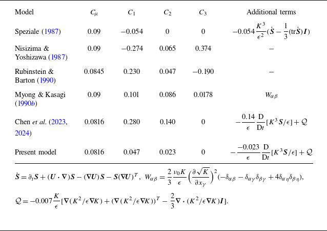
where $C_1$ , $C_2$ and $C_3$ are three empirical coefficients in traditional nonlinear models. Table 1 lists the values for these coefficients in several typical quadratic nonlinear eddy-viscosity models. The nonlinear terms derived directly from the second-order CE expansion exhibit quantitative agreement with those employed in nonlinear turbulence models. The present model incorporates additional terms that simultaneously account for both the material derivative of the strain tensor and higher-order TKE gradients, which are also considered in nonlinear turbulence models. It can be seen that the choice of $\tau = 6K/(7\epsilon )$ (Chen et al. Reference Chen, Staroselsky, Sreenivasan and Yakhot2023, Reference Chen, Staroselsky, Sreenivasan and Yakhot2024) gives higher-order transport coefficients that are larger than those of other nonlinear models, including the coefficients of the additional terms. In summary, the present kinetic model with $\tau = K/(7\epsilon )$ yields transport coefficients that are quantitatively close to those of established $K-\epsilon$ models and quadratic nonlinear eddy-viscosity models, which have been obtained empirically or semi-empirically.

4.1. Low-Reynolds-number kinetic model

In the near-wall region where the relaxation time $\tau$ is sufficiently small, the kinetic model asymptotically reduces to the linear eddy viscosity (3.8) and the gradient diffusion models (3.9). Most contemporary low-Reynolds-number $K-\epsilon$ models retain the transport-equation structure first introduced by Jones & Launder (Reference Jones and Launder1972); they differ mainly in the addition of (i) van Driest damping function $f_{\!\mu}$ , which is small within the near-wall region, and tends to unity in bulk region, and (ii) explicit molecular diffusion term $\nu _0 {\nabla} ^2K$ of which are essential to represent the strong viscous diffusion of TKE that dominates within the viscous near-wall region.

First, to incorporate the van Driest damping function $f_{\!\mu}$ explicitly into the turbulent viscosity formulation, the relaxation time $\tau$ is redefined as

(4.1) \begin{equation} \tau = \frac {f_\tau }{7}\frac {K}{\epsilon }, \quad f_\tau =\frac {7-\sqrt {49-24 f_{\!\mu} }}{2}, \end{equation}

where $f_\tau$ is a damping function corresponding to $f_{\!\mu}$ . Note that, here, the physical constraint $0 \leqslant f_\tau \leqslant 1$ is considered to ensure physically meaningful values. Substituting this into the definition of turbulent viscosity (3.9) yields

(4.2) \begin{equation} \nu _T=\frac {2\tau\! K^{eq}}{3}= C_{\!\mu} f_{\!\mu} \frac {K^2}{\epsilon }, \quad C_{\!\mu} = 0.0816. \end{equation}

A number of damping functions have been proposed. For instance, the expression proposed by Jones & Launder (Reference Jones and Launder1972) depends solely on $\textit{Re}_T$ . Subsequent refinements by Myong & Kasagi (1990a) and Nagano & Tagawa (Reference Nagano and Tagawa1990) introduce dependencies on the dimensionless wall coordinate ( $y^+$ ), thus explicitly incorporating sensitivity to near-wall length scales into the turbulence model.

Secondly, the explicit molecular viscosity diffusion $\nu _0 {\nabla} ^2K$ is incorporated by introducing an additional source term $\mathcal{S}$ into the kinetic equation

(4.3) \begin{equation} \partial _t F + \boldsymbol{\xi } \boldsymbol{\cdot }\boldsymbol{\nabla }\!F + \bar {\boldsymbol{a}} \boldsymbol{\cdot }\boldsymbol{\nabla} _{\boldsymbol{\xi }} F = \mathcal{C}_{\textit{BGK}}(F)+\mathcal{S}, \end{equation}

where $\mathcal{S}$ satisfies the following moment requirements:

(4.4) \begin{equation} \begin{aligned} &\int \mathcal{S} d\boldsymbol{\xi } = 0, \quad \int \boldsymbol{\xi } \mathcal{S} d\boldsymbol{\xi } = 0, \quad \frac {1}{2}\int \left (\boldsymbol{\xi }-\boldsymbol{U}\right )^2\mathcal{S}d\boldsymbol{\xi } = \nu _0 {\nabla} ^2K. \end{aligned} \end{equation}

There are many possible ways to design the specific form of the source term. Analogous to the formulation proposed by Lundgren (Reference Lundgren1969) for the dissipation term, we can choose

(4.5) \begin{align} \mathcal{S} = -\frac {\nu _0 {\nabla} ^2K}{2 K^{eq}} \boldsymbol{\nabla} _{\boldsymbol{\xi }} \boldsymbol{\cdot }\left [(\boldsymbol{\xi }-\boldsymbol{U})F\right ]\!. \end{align}

4.2. Wall boundary conditions

A central challenge in applying kinetic theory to turbulence is the formulation of physically consistent boundary conditions because there is no experimentally or theoretically established expression for the VDF at a solid wall. In analogy with conventional turbulence models, the wall distribution function $F(\boldsymbol{x}_w)$ is required to satisfy the following moment constraints:

(4.6) \begin{equation} \begin{aligned} &\int \boldsymbol{\xi } F(\boldsymbol{x}_w) {\rm d} \boldsymbol{\xi } = \boldsymbol{U}_w,\\ \frac {1}{2}&\int \left ( \boldsymbol{\xi } -\boldsymbol{U}(\boldsymbol{x}_w)\right )^2F(\boldsymbol{x}_w) {\rm d} \boldsymbol{\xi } = K_w,\\ \end{aligned} \end{equation}

where $\boldsymbol{x}_w$ denotes a point on the wall interface. The prescribed wall velocity $\boldsymbol{U}_w$ and TKE $K_w$ are assigned according to the turbulence model: for the LR-BGK model, they reduce to strict no-slip velocity and zero TKE, whereas for the HR-BGK model, they are supplied by empirical wall functions (Launder & Spalding Reference Launder and Spalding1983), namely the logarithmic law for velocity and the corresponding estimation of TKE.

However, different choices of $F$ can satisfy the integral constraints in (4.6), so that $F(\boldsymbol{x}_w)$ itself is not unique. A similar situation is encountered in rarefied gas from the kinetic theory, where the establishment of accurate solutions has led to a dedicated research field focused on modelling gas–surface interactions for boundary conditions (Cercignani & Lampis Reference Cercignani and Lampis1971; Cercignani Reference Cercignani1972; Lord Reference Lord1991; Aoki, Giovangigli & Kosuge Reference Aoki, Giovangigli and Kosuge2022; Kosuge et al. Reference Kosuge, Aoki, Giovangigli and Golse2025). An equally specialised effort will likely be required to develop reliable wall boundary conditions in kinetic representation of the average turbulence dynamics. Here, by leveraging boundary conditions from kinetic theory, we generalise two well-known boundary conditions of rarefied gas, namely the fully diffuse Maxwell boundary condition (Maxwell Reference Maxwell1879) and the non-equilibrium extrapolation boundary condition (Guo, Zheng & Shi Reference Guo, Zheng and Shi2002), to turbulent flows.

The fully diffuse Maxwell boundary condition (Maxwell Reference Maxwell1879) is employed in the LR-BGK model to enforce the no-slip velocity and the zero TKE at the wall. Importantly, this boundary condition produces a velocity slip and a TKE jump that both diminish linearly as $\tau$ decreases. In the near-wall region, $\tau$ is sufficiently small, so the induced slip and TKE jump are negligible, and the classical no-slip and zero-TKE limits are effectively recovered. In this boundary condition, it is assumed that particles leaving the surface follow an equilibrium VDF with the wall velocity and TKE

(4.7) \begin{equation} F(\boldsymbol{x}_w, \boldsymbol{\xi })= \alpha _w F^{eq}\left (\boldsymbol{\xi };\boldsymbol{U}_w,K_w\right )\!, \quad \boldsymbol{\xi }\boldsymbol{\cdot }\boldsymbol{n}_w\gt 0, \end{equation}

where $\boldsymbol{n}_w$ is the unit vector normal to the wall pointing to the cell, and $\alpha _w$ is the coefficient at the wall determined by the condition of zero mass flux

(4.8) \begin{equation} \int _{\boldsymbol{\xi }\boldsymbol{\cdot }\boldsymbol{n}_w\leq 0} \left (\boldsymbol{\xi }\boldsymbol{\cdot }\boldsymbol{n}_w\right )F(\boldsymbol{x}_w, \boldsymbol{\xi }) {\rm d}\boldsymbol{\xi } + \int _{\boldsymbol{\xi }\boldsymbol{\cdot }\boldsymbol{n}_w\gt 0}\left (\boldsymbol{\xi }\boldsymbol{\cdot }\boldsymbol{n}_w\right ) \alpha _w F^{eq}\left (\boldsymbol{\xi };\boldsymbol{U}_w,K_w\right ) {\rm d}\boldsymbol{\xi } = 0, \end{equation}

which gives

(4.9) \begin{equation} \alpha _w = -\frac {\int _{\boldsymbol{\xi }\boldsymbol{\cdot }\boldsymbol{n}_w\leq 0} \left (\boldsymbol{\xi }\boldsymbol{\cdot }\boldsymbol{n}_w\right )F(\boldsymbol{x}_w, \boldsymbol{\xi }) {\rm d}\boldsymbol{\xi } }{\int _{\boldsymbol{\xi }\boldsymbol{\cdot }\boldsymbol{n}_w\gt 0}\left (\boldsymbol{\xi }\boldsymbol{\cdot }\boldsymbol{n}_w\right )F^{eq}\left (\boldsymbol{\xi };\boldsymbol{U}_w,K_w\right ) {\rm d}\boldsymbol{\xi }}. \end{equation}

In practice, $K_w$ is set to a very small positive value rather than exactly zero for numerical stability.

On the other hand, for the HR-BGK model that is applicable outside the viscous sublayer, the non-equilibrium extrapolation boundary condition (Guo et al. Reference Guo, Zheng and Shi2002) in conjunction with an empirical wall function (Launder & Spalding Reference Launder and Spalding1983) is adopted. In the near-wall region, the mean velocity follows the classical logarithmic law, and the wall function is applied only inside the log layer ( $15 \lesssim y^{+} \lesssim 200$ ), bypassing the viscous sublayer

(4.10) \begin{equation} \frac {U(y)}{U_{\sigma }}= \frac {1}{\kappa }\ln \big (y^{+}\big )+B, \end{equation}

where $U_\sigma = \sqrt {\sigma _w}$ is the friction velocity obtained from the wall shear stress $\sigma _w$ with unity density, $\kappa \approx 0.41$ is the von Kármán constant and $B$ is an empirical constant; $y$ denotes the wall-normal distance measured from the wall into the fluid and $y^+=U_{\sigma }y/\nu _0$ is its dimensionless form. In addition, the corresponding wall value of the TKE is specified by the usual log-layer estimate, $K_w = U^2_\sigma /\sqrt {C_{\!\mu} }$ .

The VDF reflected from the wall located at the interface $\boldsymbol{x}_w$ is then reconstructed by the non-equilibrium extrapolation boundary condition (Guo et al. Reference Guo, Zheng and Shi2002)

(4.11) \begin{align} F(\boldsymbol{x}_w, \boldsymbol{\xi })= F^{eq}\big (\boldsymbol{\xi };\boldsymbol{U}_w,K_w\big ) - \big [ F(\boldsymbol{x}_{nc}, \boldsymbol{\xi }) - F^{eq}(\boldsymbol{x}_{nc}; \boldsymbol{U} (\boldsymbol{x}_{nc}), K (\boldsymbol{x}_{nc})) \big ], \quad \boldsymbol{\xi }\boldsymbol{\cdot }\boldsymbol{n}_w\gt 0, \end{align}

where $\boldsymbol{x}_{nc}$ is the neighbouring cell of $\boldsymbol{x}_w$ . The equilibrium term enforces the prescribed wall function moments, while the second term extrapolates the non-equilibrium part of the VDF, ensuring compatibility with the interior solution.

5.1. Numerical method and parameter set-up

As mentioned in § 2.2, the dissipation rate $\epsilon$ is an input parameter to determine the relaxation time $\tau$ in the present kinetic model. For the HR-BGK model, we adopt the widely used transport equation for the dissipation rate proposed by Launder & Spalding (Reference Launder and Spalding1983) to calculate $\epsilon$

(5.1) \begin{equation} \frac {\partial \epsilon }{\partial t} + \left ( \boldsymbol{U} \boldsymbol{\cdot }\boldsymbol{\nabla }\right )\epsilon = \boldsymbol{\nabla }\boldsymbol{\cdot }\left (\frac {\nu _T}{C_\epsilon } \boldsymbol{\nabla }\epsilon \right )+C_{\epsilon 1}\frac {\epsilon }{K}\boldsymbol{\sigma }:\boldsymbol{\nabla }\!\boldsymbol{U} - C_{\epsilon 2}\frac {\epsilon ^2}{K}, \end{equation}

where $\nu _T= 0.09 K^2/\epsilon$ , $C_\epsilon = 1.3$ , $C_{\epsilon 1} = 1.44$ and $C_{\epsilon 2} = 1.92$ . It is worth highlighting that both the TKE $K$ and the stress tensor $\boldsymbol{\sigma }$ are obtained directly from the solution of kinetic equation; therefore, (5.1) retains higher-order non-equilibrium information that is absent from the linear eddy-viscosity model. The wall boundary condition for Couette flow is implemented using a wall function approach. In this approach, the wall dissipation rate $\epsilon _w$ is prescribed based on the standard logarithmic layer estimate as $\epsilon _w = U_\sigma ^3/(\kappa y_1)$ , where $y_1$ is the wall-normal distance from the wall to the centre of the first grid cell adjacent to the wall.

Conversely, for the LR-BGK model, we employ an alternative $\epsilon$ -transport equation developed by Nagano & Tagawa (Reference Nagano and Tagawa1990), where the turbulent viscosity and model coefficients are modified as $\nu _T= 0.09 f_{\!\mu} K^2/\epsilon$ , $C_{\epsilon 1} = 1.45$ and $C_{\epsilon 2} = 1.92f_{\epsilon 2}$ . The damping functions $f_{\!\mu}$ and $f_{\epsilon 2}$ are utilised to account for near-wall damping, with their specific forms defined therein. The corresponding wall boundary condition is

(5.2) \begin{equation} \epsilon _w = \nu _0 \left (\frac {\partial \sqrt {K}}{\partial y}\right )^2\!. \end{equation}

Since the turbulent Couette flow is a quasi-one-dimensional problem, the computational cost can be reduced by introducing the following reduced distribution functions:

(5.3) \begin{equation} \left (\varPhi _1, \varPhi _2, \varPhi _3,\varPhi _4\right )^T=\int \left (1, \xi _x, \xi ^2_x,\xi ^2_z\right )^T F\left (\boldsymbol{x},\boldsymbol{\xi },t\right ) {\rm d} \xi _x{\rm d}\xi _z. \end{equation}

These reduced VDFs carry distinct essential physics in the context of turbulent transport. Here, $\varPhi _1$ represents the local mass density distribution in velocity space, directly related to the continuity equation and mass conservation, $\varPhi _2$ corresponds to the streamwise momentum distribution, governing the transport of momentum in the flow direction and thus controlling the Reynolds shear-stress generation and $\varPhi _3$ characterises the streamwise TKE distribution, which is crucial for understanding the anisotropic energy transport and the development of velocity fluctuations (or Reynolds normal stress components). Finally, $\varPhi _4$ represents the vertical kinetic energy distribution, capturing the cross-flow energy transport mechanisms. Together, these reduced VDFs encapsulate the essential physics of momentum and energy transport in wall-bounded turbulent flows while significantly reducing the computational complexity compared with the full three-dimensional kinetic equation.

The kinetic equations for the four reduced VDFs $\varPhi _k$ are solved using a discretised velocity method; further details can be found in Appendix B. To ensure accurate approximation of macroscopic moments in velocity space across various Re, computational parameters, including the spatial mesh size and the discretisation of velocity space, must be carefully selected through convergence studies until solution variations become negligible.

In our simulations, the computational domain is set to be $[-h,h]$ . For the HR-BGK model, the computational domain is uniformly discretised, with the cell size determined according to different Re. The selection criterion ensures that the first cell centre point is located inside the logarithmic layer. For the LR-BGK model, non-uniform meshes are adopted to improve the prediction by using a locally refined mesh near the boundary. The mesh points are given by $y_{\!j}/(2h)= (\zeta _{\!j}+\zeta _{j+1} )/2$ for $0\leqslant j\leqslant N_y-1$ , where $\zeta _{\!j}$ is defined by

(5.4) \begin{equation} \zeta _{\!j} = \frac {\tanh \left (a\! \left (j/N_y-1/2\right )\right )}{2 \tanh \left ( a/2\right )}, \quad j=0,1,{\cdots} ,N_y, \end{equation}

with $a$ being a dimensionless stretching parameter controlling the characteristics of the mesh distribution, and $N_y$ is the number of mesh cells. In the present study, $a$ is taken as $2.5$ . We utilise $N_y=401$ cells for the LR-BGK model, ensuring that the centre of the first off-wall cell lies within the viscous sublayer for all cases considered. The velocity space truncated at $[-5\sqrt {U_w},5\sqrt {U_w}]$ is discretised by the trapezoidal rule (Wu, Reese & Zhang Reference Wu, Reese and Zhang2014) with 4000 non-uniform velocity grid points. Furthermore, the time step is set to $0.05\times 5\sqrt {U_w}/(\Delta y_{\textit{min}})$ with $ \Delta y_{\textit{min}}$ being the minimum cell size, which satisfies the Courant–Friedrichs–Lewy condition. The steady-state solution is considered to be achieved when the maximum relative change in the velocity field between two consecutive iterations falls below $10^{-10}$ .

Figure 1.

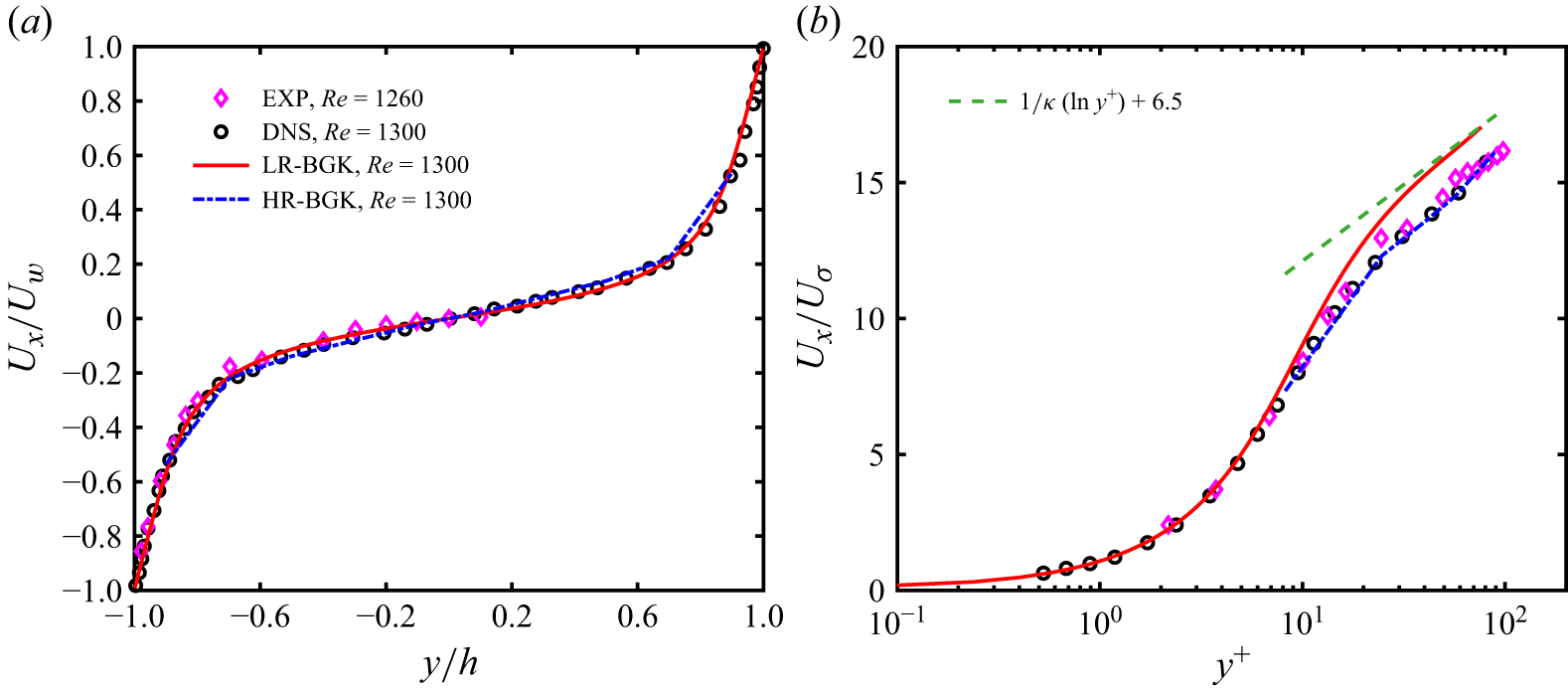
Mean velocity profiles scaled in (a) outer and (b) wall units of the turbulent Couette flow at $\textit{Re} = 1300$ .

5.2. Comparison with experiments and direct numerical simulations

The present kinetic model is validated by comparing the predictions against benchmark data from experiments and DNS solutions. The comparison focuses on key flow parameters including mean velocity profiles, dimensionless velocity distributions, skin friction coefficients and Reynolds stress components.

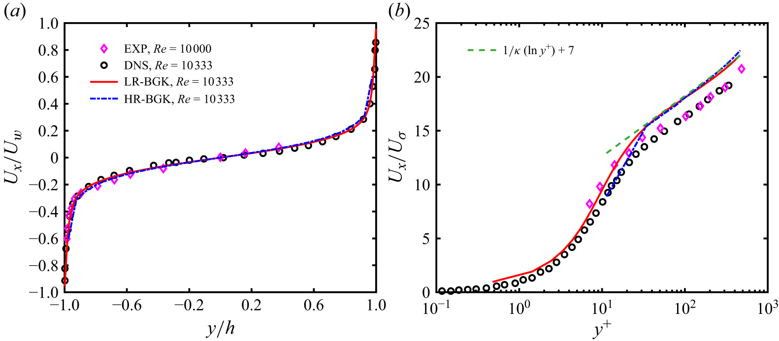
The mean velocity profiles predicted by the LR-BGK and HR-BGK models are compared with the experimental (Bech et al. Reference Bech, Tillmark, Alfredsson and Andersson1995; Robertson Reference Robertson1959b ) and DNS (Bech et al. Reference Bech, Tillmark, Alfredsson and Andersson1995; Pirozzoli, Bernardini & Orlandi Reference Pirozzoli, Bernardini and Orlandi2014) data at $\textit{Re} = 1300$ and $10\,133$ , as shown in figures 1 and 2. The results are presented in both outer units (scaled by $U_w$ and $h$ ) and wall units (scaled by $U_\sigma$ and $y^+$ ) to examine the performance of the models across different flow regions. In the case of $\textit{Re} = 1300$ , figure 1( a) demonstrates that both models accurately capture the overall velocity distribution in outer coordinates, closely matching the experimental and DNS data of Bech et al. (Reference Bech, Tillmark, Alfredsson and Andersson1995). Specifically, in figure 1( b), the HR-BGK model shows excellent agreement throughout the entire flow domain, while the LR-BGK model exhibits slightly larger deviations in the logarithmic layer. This is because HR-BGK targets the outer region (bypassing the viscous sublayer), whereas LR-BGK model includes stronger near-wall corrections that can slightly influence the log-layer profile. At a higher Reynolds number ( $\textit{Re} = 10\,133$ ), figure 2 shows that both the HR-BGK and LR-BGK models maintain their predictive accuracy, in good agreement with the experimental data of Robertson (Reference Robertson1959b ) and DNS data of Pirozzoli et al. (Reference Pirozzoli, Bernardini and Orlandi2014), although both models exhibit slightly larger deviations in the near-wall region. The logarithmic-law profile (4.10) is well captured by both models with $\kappa = 0.41$ , using $B = 6.5$ and $7.0$ for $\textit{Re} = 1300$ and $10\,133$ , respectively.

Figure 2.

Mean velocity profiles scaled in (a) outer and (b) wall units of turbulent Couette flow at $\textit{Re} = 10\,133$ .

Figure 3.

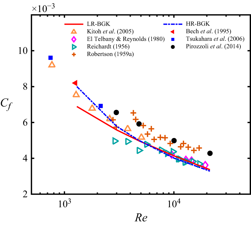
Variation of skin friction coefficient with Reynolds number.

Figure 3 presents the variation of the skin friction coefficient $C_{\!f}$ with Reynolds number, together with the comparisons with extensive experimental (Reichardt Reference Reichardt1956; El Telbany & Reynolds Reference El Telbany and Reynolds1980; Kitoh, Nakabyashi & Nishimura Reference Kitoh, Nakabyashi and Nishimura2005; Robertson Reference Robertson1959a ) and DNS (Bech et al. Reference Bech, Tillmark, Alfredsson and Andersson1995; Tsukahara, Kawamura & Shingai Reference Tsukahara, Kawamura and Shingai2006; Pirozzoli et al. Reference Pirozzoli, Bernardini and Orlandi2014) databases. The friction coefficient is defined as

(5.5) \begin{equation} C_{\!f} = \frac {\sigma _w}{\frac {1}{2}U_w^2}, \end{equation}

where $\sigma _w$ is the wall shear stress obtained directly from the VDFs. Both models demonstrate excellent agreement with the experimental data for $\textit{Re}$ between $10^3$ and $10^4$ . The LR-BGK model shows minor deviations in the lower $\textit{Re}$ range, with deviations typically less than $5\,\%$ from the data of Bech et al. (Reference Bech, Tillmark, Alfredsson and Andersson1995), Kitoh et al. (Reference Kitoh, Nakabyashi and Nishimura2005), Tsukahara et al. (Reference Tsukahara, Kawamura and Shingai2006). The HR-BGK model maintains consistent accuracy across the entire $\textit{Re}$ range, showing good agreement with both experimental and DNS data.

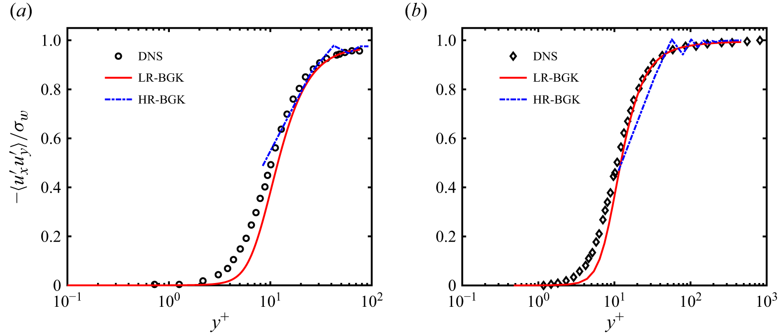
Figure 4 compares the dimensionless Reynolds shear stress $ -\langle u'_x u'_y \rangle /\sigma _w$ predicted by both kinetic models with DNS data (Bech et al. Reference Bech, Tillmark, Alfredsson and Andersson1995; Pirozzoli et al. Reference Pirozzoli, Bernardini and Orlandi2014) as $\textit{Re}$ ranges from 1300 to 10,133. It is noteworthy that the HR-BGK model, due to its coarser grid resolution, exhibits minor numerical oscillations in the near-wall region. Both kinetic models exhibit excellent agreement with the DNS data, accurately capturing both the peak value and its location, particularly in the logarithmic and outer regions ( $y^+ \gtrsim 15$ ). However, the LR-BGK model shows some deviations in the transition region ( $1 \lesssim y^+ \lesssim 15$ ) due to the inherent complexity of this region where viscous and turbulent effects compete.

Figure 4.

Reynolds shear-stress profiles scaled in wall units of turbulent Couette flow at (a) $\textit{Re} = 1300$ and (b) $\textit{Re} = 10\,133$ .

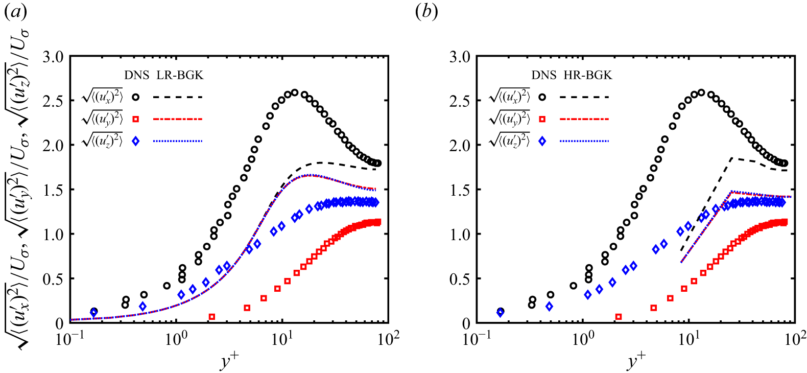
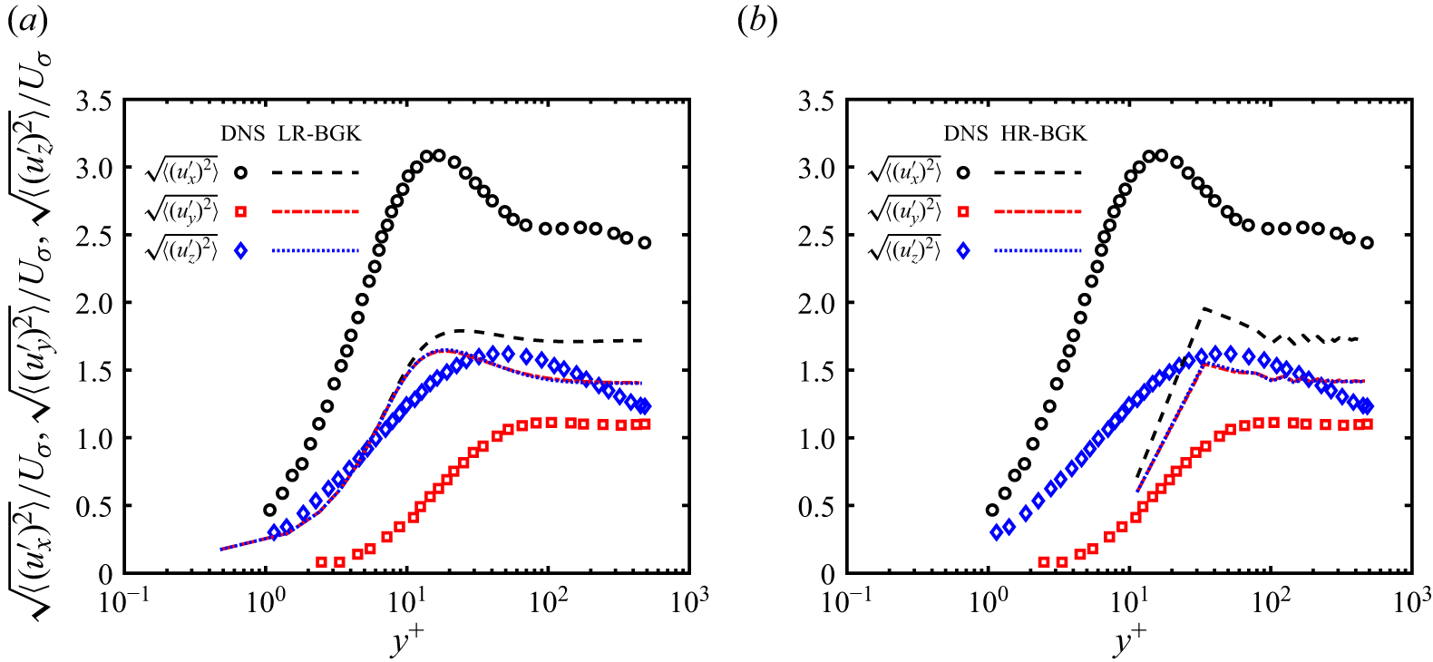
Figures 5 and 6 present detailed comparisons of the velocity fluctuation intensities (Reynolds normal stress) in all three spatial directions, providing insight into the anisotropic nature of near-wall turbulence that the linear eddy-viscosity model (3.8) fails to capture (Launder & Sharma Reference Launder and Sharma1974). The velocity fluctuation intensities predicted by the present models show noticeable differences from the DNS data (Bech et al. Reference Bech, Tillmark, Alfredsson and Andersson1995; Pirozzoli et al. Reference Pirozzoli, Bernardini and Orlandi2014), with the discrepancies becoming more pronounced at higher Re. At $\textit{Re} = 1300$ , the dimensionless streamwise $\sqrt {\langle (u'_x)^2\rangle }$ and vertical $\sqrt {\langle (u'_z)^2\rangle }$ components exhibit relatively small deviations from DNS data near the channel centreline, while the differences become increasingly evident as $\textit{Re}$ increases to $10\,133$ . The LR-BGK model demonstrates superior performance in capturing the peak locations of the streamwise fluctuations, where the peak occurs around $y^+ \approx 10$ . Notably, the largest discrepancies relative to DNS occur in the near-wall/buffer region (approximately $y^+\approx 1\sim 10$ ), where the separation among the normal stress components is underpredicted; this highlights a limitation of the present formulation and motivates further improvements. Although the magnitudes of the normal stress components are consistent with DNS, a clear separation among these components is still not reproduced by the present models. Nevertheless, they demonstrate the capability to capture non-Newtonian (nonlinear eddy-viscosity) effects, as mentioned in § 3. This non-equilibrium phenomenon, often reported in rarefied-gas flows at finite Knudsen numbers, exhibits the anisotropic stress behaviour that cannot be captured by the NS equations (Xu, Liu & Jiang Reference Xu, Liu and Jiang2007).

Figure 5.

Distribution of the velocity fluctuation intensities (Reynolds normal stress) scaled in wall units of turbulent Couette flow from (a) the LR-BGK model and (b) the HR-BGK model at $\textit{Re} = 1300$ .

Figure 6.

Distribution of the velocity fluctuation intensities (Reynolds normal stress) scaled in wall units of turbulent Couette flow from (a) the LR-BGK model and (b) the HR-BGK model at $\textit{Re} = 10\,133$ .

Figure 7.

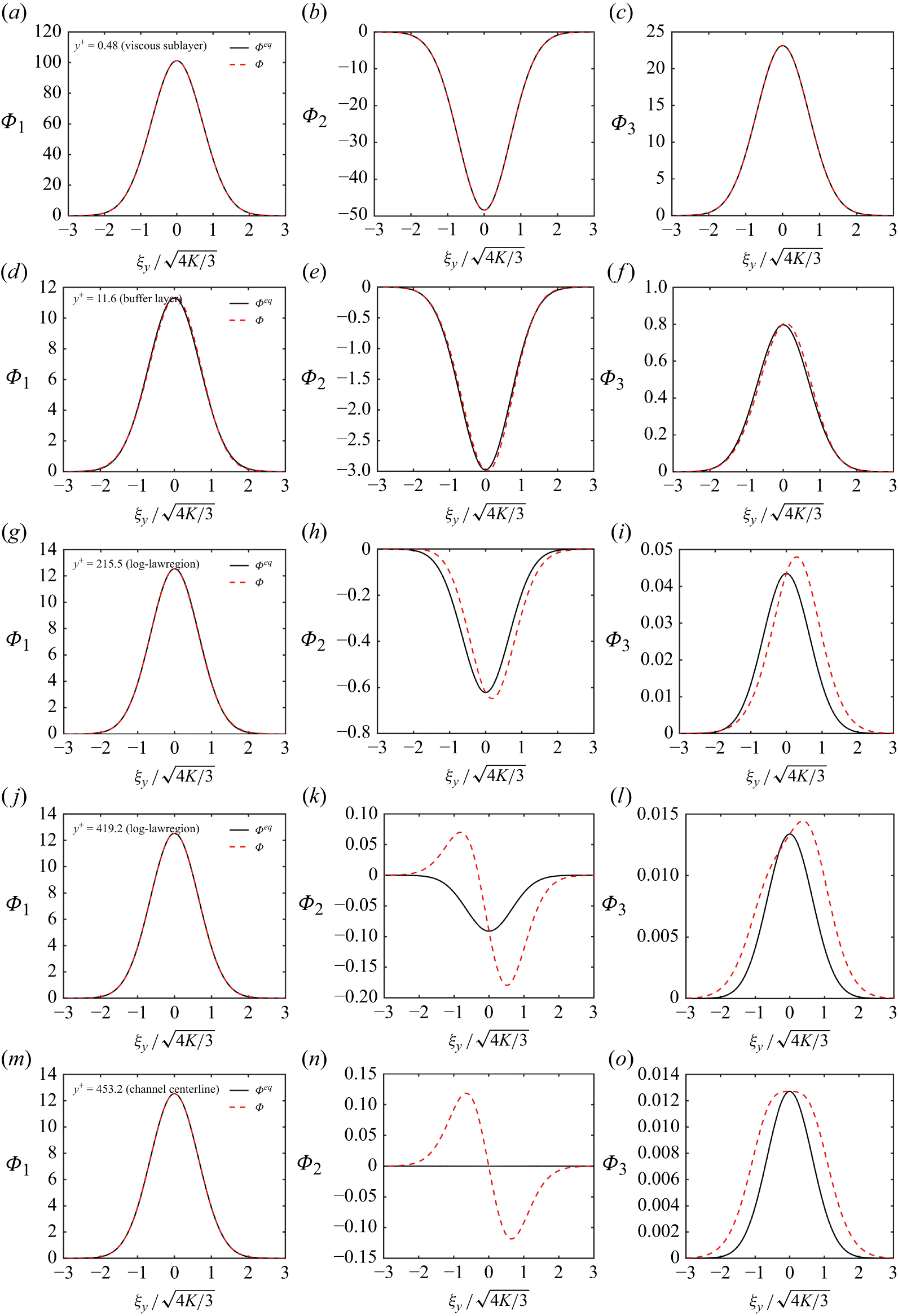
The reduced VDFs $\varPhi _1$ (a,d,g,j,m), $\varPhi _2$ (b,e,h,k,n) and $\varPhi _3$ (c, f,i,l,o) from the LR-BGK model at $\textit{Re} = 10\,133$ as a function of the microscopic velocity $\xi _y$ at different wall-normal positions.

5.3. Non-equilibrium characteristics and velocity distribution functions

The non-equilibrium and non-Newtonian characteristics predicted by the present kinetic model can be essentially explained from the VDFs. We now examine the reduced VDFs obtained from the LR-BGK model at $\textit{Re}=10\,133$ , comparing the computed VDFs with their corresponding local equilibrium distributions to quantify the degree of departure from equilibrium. Figure 7 presents the reduced VDFs $\varPhi _1$ , $\varPhi _2$ and $\varPhi _3$ as functions of microscopic velocity $\xi _y$ in various normal wall positions ranging from the viscous sublayer to the centreline of the channel, compared against the local equilibrium VDFs derived from the local mean velocity and TKE. Here, $\xi _y$ in the region $ [-3\xi _m,3\xi _m ]$ with $\xi _m = \sqrt {4K/3}$ represents the most probable velocity scale based on the local TKE. The fourth VDF $\varPhi _4$ exhibits behaviour similar to $\varPhi _1$ by remaining close to equilibrium; it is therefore omitted here for brevity.

The most striking observation is the markedly different behaviours exhibited by the various reduced VDFs. The distribution function $\varPhi _1$ , which represents the zeroth-order moment in the wall-normal direction, remains remarkably close to its local equilibrium state across all wall-normal positions. This near-equilibrium behaviour indicates that the mass conservation constraint is well satisfied throughout the flow domain, consistent with the incompressibility condition. In sharp contrast, $\varPhi _2$ and $\varPhi _3$ exhibit pronounced departures from their respective equilibrium distributions, particularly in the outer region of the flow. Here, the ‘equilibrium’ baseline refers to the local isotropic Gaussian distribution $F^{eq}$ (and its reduced counterparts $\varPhi ^{eq}_k$ ) constructed from the local mean velocity and TKE. Therefore, the deviations primarily reflect shear-induced anisotropy and wall-normal inhomogeneity in the averaged turbulence dynamics. The VDF $\varPhi _2$ , associated with the streamwise momentum transport, shows increasing non-equilibrium effects as the distance from the wall increases. Notably, at $y^+ \approx 419$ and near the channel centreline, $\varPhi _2$ exhibits a clear departure from the isotropic Gaussian baseline, characterised by an odd-in- $\xi _y$ (sign-changing) deviation. This feature is directly related to the Reynolds shear stress, since $\sigma _{xy}=-\langle u_x' u_y'\rangle$ is obtained as the moment of the reduced distribution (in our definition, $\sigma _{xy}=-\int \xi _y \varPhi _2 d\xi _y+U_x U_y$ for $U_y\approx 0$ ). The observed positive deviation for $\xi _y\lt 0$ and negative deviation for $\xi _y\gt 0$ contributes to the negative correlation $-\langle u_x'u_y'\rangle$ , consistent with the leading-order (first-order CE) closure and also with linear eddy-viscosity modelling. Similarly, $\varPhi _3$ , which is related to the streamwise kinetic energy transport, demonstrates substantial non-equilibrium characteristics with a comparable spatial evolution pattern. The VDF $\varPhi _3$ shows progressively stronger departures from equilibrium as the wall-normal distance increases, with the outer region exhibiting the most pronounced non-equilibrium effects. At $y^+ \approx 419$ and near the channel centreline, $\varPhi _3$ exhibits a clear asymmetry/shift relative to the isotropic baseline. This feature indicates a nonzero wall-normal transport of TKE flux, which corresponds to a higher-order velocity moment of the VDF and is captured at leading order by the first-order CE closure.

While the leading-order trends of these effects can be understood qualitatively within the first-order CE closure, we further quantify the degree of departure from equilibrium and assess the contributions beyond the first-order closure by examining the second-order moment of $F-F^{eq}$

(5.6) \begin{equation} \boldsymbol{\sigma }^{\textit{neq}}=-\int \left (\boldsymbol{\xi }-\boldsymbol{U}\right )\left (\boldsymbol{\xi }-\boldsymbol{U}\right ) (F-F^{eq})d\boldsymbol{\xi }. \end{equation}

It should be noted that the zeroth- and first-order moments of $F-F^{eq}$ vanish identically. In the case of plane Couette flow, (3.12) reduces to

(5.7) \begin{equation} \begin{aligned} \sigma ^{\textit{CE}}_{xy}&=\nu _T\frac {\partial U_x}{\partial y},\\ \sigma ^{\textit{CE}}_{xx}&=-\frac {2}{3}K-\frac {2\nu _T^2}{K^{eq}}\left (\frac {\partial U_x}{\partial y}\right )^2+\frac {2 \nu _T}{3K^{eq}}\frac {\partial }{\partial y} \left (\nu _T\frac {\partial\! K^{eq}}{\partial y}\right )\!,\\ \sigma ^{\textit{CE}}_{yy}&=-\frac {2}{3}K+\frac {\nu _T^2}{K^{eq}}\left (\frac {\partial U_x}{\partial y}\right )^2-\frac {4\nu _T}{3K^{eq}}\frac {\partial }{\partial y} \left (\nu _T\frac {\partial\! K^{eq}}{\partial y}\right )\!,\\ \sigma ^{\textit{CE}}_{zz}&=-\frac {2}{3}K+\frac {\nu _T^2}{K^{eq}}\left (\frac {\partial U_x}{\partial y}\right )^2+\frac {2\nu _T}{3K^{eq}}\frac {\partial }{\partial y} \left (\nu _T\frac {\partial\! K^{eq}}{\partial y}\right )\!. \end{aligned} \end{equation}

where $\nu _T = 0.0816 f_{\!\mu} K^2/\epsilon$ . These expressions indicate significant differences among the three normal stress components, demonstrating the capability of the present kinetic model to capture anisotropic stress behaviour.

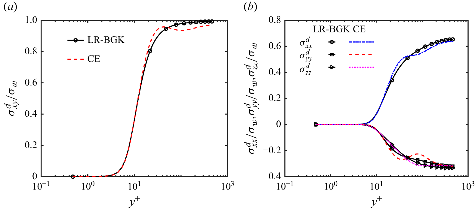
Figure 8 presents the deviatoric part of $\boldsymbol{\sigma }^{\textit{neq}}$ predicted by LR-BGK model at $\textit{Re}=10\,133$ , and compares the results with the CE expansion results given by (3.12). It can be seen that the deviatoric Reynolds stress shows good agreement between the LR-BGK model and the CE expansion throughout the flow domain, validating the theoretical consistency of the kinetic approach. The minor discrepancies observed can be attributed to higher-order terms in the CE expansion that are not captured by the second-order analysis. Furthermore, the deviatoric Reynolds normal stress components better reflect the degree of departure from non-equilibrium of the VDFs mentioned above. In the present model calculations, the deviatoric normal stress components remain close to zero in the viscous sublayer. Across the buffer region, they begin to deviate from zero, with $\sigma ^{d}_{xx}$ increasing to positive values while $\sigma ^{d}_{yy}$ and $\sigma ^{d}_{zz}$ decrease to negative values. Their magnitudes continue to grow toward the outer layer, where the non-equilibrium signatures become more evident. This relatively weak near-wall non-equilibrium signature may also reflect a limited capability of the present formulation to represent buffer-layer non-equilibrium effects, which could contribute to the relatively large discrepancies in the normal stress predictions observed in figure 6 in the near-wall region ( $1 \lesssim y^+ \lesssim 10$ ) compared with DNS data. A possible cause is that, especially in the near-wall region, the relaxation time $\tau$ in the present single-relaxation-time BGK closure is chosen for obtaining the desirable shear stress, as a result, the effective turbulent Knudsen number ( $\sim \tau |S|$ ) becomes too small, so that all other Reynolds stress components are suppressed. One of the future investigations is how to adjust $\tau$ to match shear stress without sacrificing the non-equilibrium effects for normal stress components, including generalisation of the single-relaxation-time collision model to involve multiple relaxation times.

Taken together, the VDFs and their associated non-equilibrium moments provide a framework-specific interpretation for the ability of the present kinetic models to represent anisotropic Reynolds stress behaviour and related non-Newtonian effects. Within this interpretation, departures from local equilibrium reflect finite-relaxation effects in the kinetic closure, analogous in spirit to non-equilibrium transport in rarefied-gas kinetics.

Figure 8.

Deviatoric Reynolds (a) shear-stress component and (b) normal stress components in wall units of turbulent Couette flow at $\textit{Re} = 10\,133$ . Here, the deviatoric Reynolds stress is defined as $\boldsymbol{\sigma }^d=\boldsymbol{\sigma }- {1}/{3} (\text{tr}\boldsymbol{\sigma }) \boldsymbol{I}$ .