


1. Introduction
Autonomous indoor navigation in residential or commercial spaces requires efficient path planning under a variety of operational and computational constraints [Reference El-Sheimy and Li1–Reference Hichri, Gallala, Giovannini and Kedziora3]. Autonomous unmanned ground vehicles, for instance, require efficient path planning to navigate around walls and other obstacles en route to their destinations. Classical path planning algorithms such as A* [Reference Hart, Nilsson and Raphael4, Reference Sathyaraj, Jain, Finn and Drake5], Anytime Repairing A* (ARA*) [Reference Likhachev, Gordon and Thrun6], and Rapidly Exploring Random Tree* (RRT*) [Reference Karaman and Frazzoli7] search over the space of feasible paths, but their performance is tightly coupled to the topology and size of the environment. In environments with extensive free space and numerous obstacles, computational costs become prohibitive due to the increased complexity of navigation and path planning [Reference Noreen, Khan and Habib8]. Learning-based approaches [Reference Pfeiffer, Schaeuble, Nieto, Siegwart and Cadena9] propose tackling this problem by directly mapping sensory and robot-state inputs to motion commands or trajectories that reach a single target. We instead present MazeNet, a method for intelligent search-space reduction that targets multigoal shortest-path planning. MazeNet operates on a discretized, maze-like graph/image abstraction and serves only to reduce the search space for downstream classical planners, rather than learning from raw sensor observations or outputting robot controls.
Path quality comparison in a three-terminal maze (green squares). The exact method finds the optimal shortest path (blue), while the approximation yields a suboptimal solution (red); cross-hatching denotes overlap.

Figure 1. Long description
Panel A: A maze with a blue path indicating the optimal shortest route from the start to the green squares. Panel B: The same maze with a red path showing a suboptimal solution. Cross-hatching in both panels denotes overlapping areas between the paths.
To make complex environments more tractable for path planning, one can consider an abstraction of free space into a two-dimensional (2D) grid graph, where each node corresponds to a uniformly spaced location that is connected to its four cardinal neighbors. We remove any node or edge that lies inside an obstacle from the graph. This representation forms a maze-like graph, enabling the path-planning problem to be approached using algorithms informed by maze-solving results in graph theory. Maze-solving algorithms have long served as foundational tools for solving the Obstacle-Avoiding Rectilinear Steiner Minimum Tree (OARSMT) problem and other graph combinatorial optimization tasks [Reference Lin, Lin, Li and Lin10]. OARSMT’s goal is to connect a set of predefined destinations, called terminals, using shortest paths that avoid obstacles, a feature inherent to indoor environments. The terminals are unordered, meaning that there is no predefined sequence of visitation. OARSMT has applications in integrated circuit design [Reference Kahng, Lienig, Markov and Hu11], network routing [Reference Dong, Zhu, Xie and Zeng12], and multipath planning for robotics [Reference Choset, Lynch, Hutchinson, Kantor, Burgard, Kavraki and Thrun13, Reference Zang, Yin, Huang, Yu, Zonouz and Yuan14]. In these contexts, even small gains in runtime or path length can yield operationally important savings in cost and energy, particularly in multitarget robot navigation scenarios [Reference Bricaud15].
OARSMT is NP-complete [Reference Garey and Johnson16], and while approximation algorithms offer good scalability, they generally fail to find optimal shortest solutions, even on simple problems. These approximation algorithms scale polynomially with the number of terminals and, on the other hand, near-linearly with the number of nodes. Exact methods scale factorially with the number of terminals due to permutation complexity and polynomially with the number of nodes due to shortest-path computations. Therefore, for OARSMT, computational difficulty is driven mainly by the number of terminals rather than the number of nodes. In this work, we operate on a problem scale with regard to the number of terminals and room sizes where computing exact solutions remains feasible, though expensive, and approximation methods are prone to mistakes. Even for an 11 × 11 node grid size and 3 terminals, approximate methods routinely make mistakes, as Figure 1 shows, where an approximation fails to find the minimal tree while the exact method succeeds.
To address the issue of accuracy while still maintaining fast runtimes, we introduce a search-space reduction pipeline (SRP), a complete pipeline for path planning that integrates an RCNN module, which we refer to as MazeNet, as its core learning component for the graph-theoretic OARSMT. MazeNet predicts a rectilinear tree constrained to the cardinal directions north–west–south–east (NWSE) that defines a corridor path through the environment. As Figure 2 shows, SRP converts the floor plan into a grid graph, transforms it into a maze-like image processed by MazeNet, and finally reinterprets the output as a constrained corridor mask that guides the path planner within the environment.
MazeNet’s design draws inspiration from a technique known as “deep thinking” [Reference Schwarzschild, Borgnia, Gupta, Huang, Vishkin, Goldblum and Goldstein17]. This technique utilizes a recurrent convolutional neural network (RCNN) and a tailored training procedure to extend from simple to complex problem instances. In our case, MazeNet trains to solve indoor navigation tasks with a limited number of destinations and extends this capability at inference time by performing additional iterations, enabling empirically accurate and efficient solutions to higher-complexity instances of a problem for which no efficient classical algorithm is known, without requiring retraining.
Unlike classical methods that operate directly on high-resolution floor plans, MazeNet works by design on a lower-resolution grid view that serves as a corridor map, constraining the search space while remaining fine enough to capture connectivity of the environment to find valid shortest paths. We detail the graph–image mapping in Section 3.2 to give a clear picture of how a graph appears as a maze and a solution tree as a corridor. MazeNet achieves optimal shortest paths for realistic problem scales while reducing planning runtime. Experiments on synthetic mazes and, after fine-tuning MazeNet, on both self-generated and real-world floor plans demonstrate these gains. Physical feasibility of the constrained paths is further validated in a PyBullet [Reference Coumans18] physics simulation using a TurtleBot-class robot [Reference Amsters and Slaets19], confirming that search-space reduction preserves safe and collision-free navigation.
High-level overview of the proposed search-space reduction pipeline (SRP): constrains the environment for accelerating path planning.

We organize the paper as follows. Section 2 reviews prior work related to OARSMT, classical graph algorithms, and learning-based approaches for path planning. Section 3 formally defines OARSMT, reviews its computational complexity, and describes the specific variation addressed in this paper. Section 4 describes the MazeNet architecture and training process. Section 5 extends SRP to practical path planning applications using MazeNet-derived masking filters. In Section 6, we compare SRP to state-of-the-art alternative methods in terms of accuracy, path length, and runtime, and validate the physical feasibility of the constrained paths in robot simulation. Finally, Section 7 concludes the paper and discusses potential directions for future research.
2. Prior work
Path planning has been extensively studied, with comprehensive surveys categorizing methods by their completeness and optimality guarantees [Reference Hoy, Matveev and Savkin2, Reference Goerzen, Kong and Mettler20, Reference Lopez, Zapata and Osorio-Lama21]. Classical approaches include graph search methods such as A* and replanning variants like ARA* [Reference Sathyaraj, Jain, Finn and Drake5], sampling-based planners such as RRT and asymptotically optimal extensions [Reference Karaman and Frazzoli7, Reference Ayawli, Dawson, Badu, Ayawli and Lamusah22, Reference McMahon, Sivaramakrishnan, Granados and Bekris23], optimization-based formulations commonly used within Model Predictive Control frameworks [Reference Richards and How24], and heuristic or stochastic trajectory optimization methods including evolutionary approaches [Reference Zheng, Li, Xu, Sun and Ding25–Reference Sharma and Voruganti27]. Despite their differing representations and guarantees, many of these methods scale with environment size and therefore benefit from reducing the search space. MazeNet performs this reduction by solving a non-trivial graph problem derived from the environment.
Researchers typically address nontrivial graph problems using one of two approaches: exact algorithms that guarantee optimality but become intractable in large or cluttered environments, and approximation algorithms that improve scalability at the cost of potential sub-optimality in path length. We thoroughly characterize MazeNet’s performance by comparing it against three classical approximation algorithms for solving OARSMT instances: the algorithm by Kou et al. [Reference Kou, Markowsky and Berman28], Mehlhorn’s algorithm [Reference Mehlhorn29], and Wavefront Minimum Spanning Tree (Wavefront MST) [Reference Prim30]. To obtain exact solutions, Dijkstra’s algorithm [Reference Cormen, Leiserson, Rivest and Stein31] is well-suited when there are only two terminals to connect. However, when connecting more than two terminals, finding the minimal obstacle-avoiding tree becomes a combinatorially difficult problem. On relatively small floor plans, we evaluate all permutations of terminal connections and select the one with the lowest total length to obtain exact solutions. We refer to this algorithm as Multi-terminal Dijkstra (MT-Dijkstra).
To overcome the various limitations of existing classical and approximate methods, recent machine learning approaches have explored hybrid solutions for Steiner-type problems. For example, [Reference Kahng, Nerem, Wang and Yang32] proposes a neural-algorithmic model, though it neglects obstacles. Other works [Reference Chen, Ke, Lee, Tsai, Kung, Lin, Liu, Chang, Li and Chao33–Reference Chu and Wong36] focus on scalability in the field of very-large-scale integration (VLSI) layout design, rather than for performance in indoor environments. Because these methods consider geometric and obstacle constraints only in a limited way, they remain inapplicable to indoor environments.
Recent learning-based approaches in robotics typically address different problem settings than ours. End-to-end methods, such as DeepMoTIon [Reference Hamandi, D’Arcy and Fazli37] and perception-to-decision pipelines [Reference Pfeiffer, Schaeuble, Nieto, Siegwart and Cadena9], learn direct mappings from sensor observations and robot states to formulate motion commands toward a single target. Latent-space planning approaches, such as learned sampling-based motion planning [Reference Ichter and Pavone38], focus on accelerating high-dimensional single-goal planning; however, they still rely on stochastic sampling and do not aim to preserve exact shortest-path solutions. More recent graph-learning methods, including KG-Planner [Reference Liu, Eltouny, Tian, Liang and Zheng39], target high-dimensional manipulator motion in dynamic or collaborative settings, prioritizing feasibility over exact optimality guarantees. As a result, these methods operate under different assumptions and objectives than ours.
Graph convolutional networks have also been applied to related decision-making tasks [Reference Li, Chen and Koltun40], and reinforcement learning methods have been used to find approximate solutions to problems like the Traveling Salesman and Vehicle Routing Problems [Reference Kool, van Hoof and Welling41]. These approaches typically target large-scale graphs with thousands or millions of nodes and focus on approximate solutions. In contrast, prior optimal methods [Reference Osanlou, Bursuc, Guettier, Cazenave and Jacopin42] are limited to graphs with fewer than 25 nodes and evaluate under 20 configurations, typically by varying only the terminal locations for the same graph. MazeNet is instead trained on 500,000 distinct graphs, each with different sets of terminals, enabling adaptability across a much wider distribution of graph examples and serving as a learned preprocessing module for downstream planners.
While graph space simplification, maze-style image representations, and RCNNs [Reference Liang and Hu43] are each individually well-established techniques, combining these components sequentially for learning to extract optimal path masks is, to the best of our knowledge, a novel formulation. Prior RCNN-based methods [Reference Schwarzschild, Borgnia, Gupta, Huang, Vishkin, Goldblum and Goldstein17, Reference Bansal, Schwarzschild, Borgnia, Emam, Huang, Goldblum and Goldstein44] addressed maze-solving tasks with only two terminals, focusing on domains where traditional graph methods are both fast and accurate. MazeNet extends this approach to multiple terminals by training on exact solutions that we obtain from MT-Dijkstra. The approaches in refs. [Reference Schwarzschild, Borgnia, Gupta, Huang, Vishkin, Goldblum and Goldstein17] and [Reference Bansal, Schwarzschild, Borgnia, Emam, Huang, Goldblum and Goldstein44] first bridged the gap between RCNNs and graph-theoretic methods. However, researchers have not yet explored the potential of RCNNs for solving more complex graph problems, and MazeNet addresses this gap.
3. Problem statement
3.1. OARSMT
At the heart of SRP is MazeNet, a solver for a specific family of OARSMT problems derived from floor plans. OARSMT seeks to connect a set of terminals using only horizontal and vertical line segments (rectilinear paths) while avoiding rectangular obstacles, with the goal of minimizing the total length of the tree. OARSMT is formally defined as follows:
Given a set of terminals
 $ {T} \triangleq \{ t_1,\ldots ,t_N \}$
in the plane, where
 $ t_i=(x_i,y_i)$
, and a set of rectangular obstacles
 $ {O} \triangleq \{ O_1,\ldots , O_m \}$
, where
 $ O_j$
has opposite vertices
 $ (x_{j\min },y_{j\min })$
and
 $ (x_{j\max },y_{j\max })$
, let
 $ {\boldsymbol{\mathcal{S}}({T},{O})}$
denote the set of rectilinear (axis-aligned), obstacle-avoiding, connected, acyclic trees that span
 $ {T}$
. For any tree
 $ {S}$
, let
 $ {E({S})}$
denote the set of its edges and let
 $ {\ell }$
denote the edge-length function, so that for each edge
 $ e_k \in {E({S})}$
,
 $ {\ell }(e_k)$
is the length of the corresponding edge. Let
 $ {L}$
denote the total-length functional on trees that sums the lengths of the edges in
 $S$
, defined by
 $ {L}({S}) \triangleq \sum _{e_k \in {E({S})}} {\ell }(e_k)$
. Solving OARSMT means solving an optimization problem that finds the tree
 $S^\star$
such that:
 \begin{equation} {S^\star } = \mathop{\operatorname{argmin}}\limits_{{S} \in {\boldsymbol{\mathcal{S}}({T},{O})}} {L}({S}). \end{equation}
By construction,
 $ {S^\star }$
is connected and acyclic, spans all terminals in
 $ {T}$
, every edge
 $ e_k \in {E({S^\star })}$
is rectilinear, and no edge intersects the interior of any
 $ O_j \in {O}$
. Since the graphs that we will be working with come from equally spaced grid graphs; we can take, for any tree
 $S$
,
 $ {\ell }(e_k) \equiv 1$
for all
 $ e_k \in {E({S})}$
, hence
 $ {L}({S}) = \lvert {E({S})} \rvert$
. Equivalently, the problem reduces to minimizing the edge count.
Although the classic Steiner Tree Problem is already NP-complete, OARSMT is even more computationally demanding due to the additional obstacle-avoidance constraints. The optimization searches over sets of valid trees that remain connected, acyclic, span all terminals, and avoid obstacles. The search space is discrete and heavily constrained, making exact optimization difficult and often impractical even for small graphs or terminal configurations.
To analyze the computational complexity of obtaining exact solutions for OARSMT instances, we adopt the previously introduced exhaustive combinatorial strategy MT-Dijkstra, which computes optimal obstacle-avoiding rectilinear trees for small graphs [Reference Laporte45]. Given a set of
 $N$
terminals, we evaluate all
 $N!$
permutations of the
 $N$
terminals and sequentially connect terminals using the shortest obstacle-avoiding path between each consecutive pair, computed via Dijkstra’s algorithm [Reference Cormen, Leiserson, Rivest and Stein31]. Each path computation has time complexity
 $\mathcal{O}(V \log V)$
, where
 $V$
is the number of nodes in the grid, resulting in a total complexity of
 $\mathcal{O}(N! \cdot (V+1) \log V)$
. To ensure that the result forms a tree, we apply a tie-breaking rule that favors paths avoiding invalid cycles. This algorithm produces a permutation-based, minimum-length, connected, and acyclic tree. Although the overall algorithm runs in factorial time, it remains tractable for small
 $N$
(e.g.,
 $N \leq 8$
). MT-Dijkstra is exact within this formulation because each pairwise connection is computed over the full graph, including the exhaustive evaluation of all
 $N!$
terminal orderings, which identifies the minimum-length tree. When multiple permutations produce the same minimum edge count, the tie-breaking rule selects the first computed solution as the training target. We use this exact solver both to benchmark and to generate ground-truth solutions for OARSMT instances.
3.2. Graph-to-image mapping
To enable RCNN-based processing with MazeNet within SRP, we convert the discretized floorplan graph into an image that preserves connectivity, obstacles, and terminals. The transformation from a graph to an image assumes that nodes and edges lie on integer coordinates of a 2D unweighted grid. We introduce a simple mapping from a 2D grid graph to an image: each node and edge in the graph are associated with a fixed location on the 2D grid and can therefore be mapped to a distinct cell in an image. Because the graph is unweighted and rectilinear, every node or edge has a well-defined
 $(x, y)$
coordinate. We assign a
 $2 \times 2$
cell of pixels to each node or edge cell. If the node or edge exists in the graph, its corresponding pixel cell is set to white; otherwise, it is rendered in black. This process creates a binary image representation of the graph.
As shown in Figure 3, an
 $11 \times 11$
grid of nodes yields a
 $21 \times 21$
arrangement of alternating nodes and edges. After assigning
 $2 \times 2$
pixels per cell and adding a 3-pixel padding on all sides, the final image size is
 $48 \times 48$
pixels. Nodes that are selected as terminals can be color-coded in green in the final image. Because all terminals have equal importance, we encode them identically in a single-color channel (green in our implementation). The specific color is arbitrary, but this single-color terminal encoding is a novelty introduced by MazeNet that we found was vital for obtaining correct multiterminal solutions. This generated image preserves the structure and connectivity of the original graph. Similarly, any tree defined on the same graph can be visualized as a path mask using the same transformation. Figure 3(b) shows the image representation of an optimal tree computed on the underlying graph image, and Figure 3(c) shows the optimal shortest tree in isolation as the binary mask image serving as the target for supervised training. This process defines a consistent and general mapping between grid-embedded graphs and images.
Graph-to-image conversion: example of converting a graph (a) to its corresponding image representation with the solution imposed for clarity (b), with the solution image (c) as its shortest-path target.

Figure 3. Long description
Panel A: A graph representation with blue nodes and green target nodes. Panel B: An image representation of the graph with a maze-like structure and a blue path indicating the solution. Panel C: The solution image showing the shortest path in white against a black background.
Images that represent navigable environments, such as floor plans, can also be discretized into graphs. This floorplan-graph mapping proceeds by discretizing the image into an evenly spaced 2D rectilinear grid of unit cells, preserving unweighted, axis-aligned edges. The choice of unit cell size is operationally relevant: we select the largest possible unit cell that ensures the resulting graph preserves the connectivity of the free space, thereby capturing the structure while minimizing complexity. Each traversable unit cell (node or edge) in the image is mapped to a white cell, while non-traversable unit cells (obstacles) are mapped to black cells. Detailed graph generation steps are provided in Appendix A.1. This approach provides a flexible and scalable way to create graph-image pairs.
4. MazeNet
We now present MazeNet, the RCNN module within SRP, starting with its RCNN building blocks and architecture in Section 4.1. In Section 4.2, we introduce the termination condition (TC) module and present its algorithm in detail. Finally, in Section 4.3, we present MazeNet’s training procedure.
4.1. RCNN approach
RCNN, which applies convolution operations recurrently and is widely used in image recognition tasks, forms the backbone of MazeNet. A high-level overview of the MazeNet architecture is shown in Figure 4. The architecture of MazeNet builds upon the RCNN design introduced in ref. [Reference Bansal, Schwarzschild, Borgnia, Emam, Huang, Goldblum and Goldstein44], which the authors originally developed to connect two terminals in perfect mazes, i.e., mazes with a unique shortest path solution between any two nodes. MazeNet uses three main components from the architecture in ref. [Reference Bansal, Schwarzschild, Borgnia, Emam, Huang, Goldblum and Goldstein44]:
High-level overview of the MazeNet architecture, detailing the convolutional modules responsible for processing the input maze and generating the output mask.

A Projection module, a Batch module that applies a recurrent block (RB) for multiple iterations, and a final Head module. The Projection module receives a 3-channel RGB input image and projects it to a fixed-width representation, enabling the Batch module to operate independently of the input image size. The Batch module operates iteratively, receiving a stacked input consisting of the projected feature map and the original image through a skip connection. The output of the Batch module maintains a fixed width, which is a tunable hyperparameter. Finally, the Head module maps the Batch module output to two output channels, and an argmax operation over these channels produces the binary prediction. In this work, we adapt MazeNet to handle multiple terminals and more complex environments. MazeNet combines the Projection, Batch, and Head modules, along with the TC detailed in Section 4.2, and the training procedure described in Section 4.3. Appendix A.2 provides detailed descriptions of each module.
MazeNet’s progress over time as it connects five terminals with the shortest overall path in a typical 11 × 11 maze. The sequence demonstrates the successful identification of the shortest overall path.

RCNNs offer step-by-step interpretability because their image outputs can be visualized at each iteration. This enables us to observe the intermediate stages toward the solution. In MazeNet’s case, these intermediate stages are mazes, which help us to understand the operation of the learned maze-solving algorithm. Figure 5 illustrates MazeNet’s behavior: after suppressing the white permissible paths of the maze in the input image, exploratory paths originate from the terminals, which intensify and become stable once the correct terminal connections are established. These image frames help reveal how the network incrementally builds the solution, providing a way to detect failure modes by observing when paths fail to connect or converge incorrectly.
4.2. Termination condition block
The RCNN architecture of ref. [Reference Bansal, Schwarzschild, Borgnia, Emam, Huang, Goldblum and Goldstein44] does not include any TCs, so we must predefine the number of recurrent iterations. This can lead either to premature termination that ends the algorithm without yielding the correct shortest path or to excessive runtimes due to unnecessary steps taken after the algorithm has already reached the correct solution. As the example maze in Figure 5 shows, the correct path is already visually clear by the 23rd iteration, even though the output has not fully converged to a solidly white path. Therefore, an unmodified application of existing RCNN methods to indoor path planning results in excessive and uncompetitive runtimes. This observation motivates the introduction of the TC module, which can automatically detect when the maze is essentially solved and return the current shortest path as the final prediction. The TC module is our central contribution: it turns an open-ended RCNN into a method that stops itself when the solution is ready, resolves near-tie oscillations, prevents unwanted iterations, and preserves accuracy. This capability is general and can carry over to other RCNN applications that produce interpretable intermediate outputs.
Another limitation of existing RCNNs that we have discovered is their tendency to oscillate between multiple nearly equivalent solutions when two or more paths have similar lengths. In such cases, the output may alternate between these paths, and the network may fail to select the actual shortest path, resulting in an incorrect solution. Figure 6 shows an example of this behavior, where the correct path appears intermittently during oscillation but is not consistently predicted. The TC module addresses this shortcoming by explicitly detecting when ties occur and resolving them accurately. In doing so, the TC module ensures that the network selects the true shortest path and avoids redundant computation.
We do not apply TC after every RB iteration because it is runtime-intensive; instead, MazeNet applies the module after batches of RB modules to limit overhead while maintaining accuracy. The first Batch module includes 20 RB iterations; subsequent Batch modules include 10. After each batch, the TC module (Algorithm 1) follows the head module and performs a search starting at the upper-leftmost terminal and proceeding along white pixels to check for path connectivity. The argmax operation over the two Head channels is applied separately to obtain the final binary prediction used for accuracy evaluation, as detailed in Appendix A.2. We define “path intensity” as the continuous value from the Head’s soft, pre-argmax channel-1 output, clamped to
 $[0,1]$
. The TC module specifically evaluates the path intensity in a
 $ 2 \times 2$
neighboring cell grid, averaging the 0–1 value of the four pixels at the neighboring cell (line 8). If the path intensity exceeds an empirically determined threshold, selected on a held-out validation set and then fixed before evaluating the test sets, TC continues the exploration in any direction – North, West, South, or East – above the threshold. As it moves, it tracks visited positions (line 6), the number of terminals reached, and ensures the output does not contain cycles. Appendix A.11 provides a TC module sensitivity analysis over the range
 $[0.30, 0.80]$
.
Resolution of equidistant paths: visualization of progress when a termination condition is needed to resolve between two almost equidistant paths, as prior RCNNs would otherwise oscillate between them.

When encountering a junction where multiple directions exceed the path intensity threshold, TC initiates a recursive branch of exploration while keeping track of the main branch using a Boolean variable, from_junction, which we introduce to distinguish whether the current branch originates from a junction (line 17). Since the predicted output must form a valid tree, we use recursion to explore each branch, as this is a natural and structured way to traverse tree-like graphs (line 21). Although recursive methods are runtime-intensive, they are acceptable for the graph sizes that we use in this work and guarantee full tree exploration. If a branch leads to a previously visited position, indicating a cycle, the TC module stops (lines 5, 19) and runs additional convolutional RB module iterations on the image to ensure valid tree convergence. TC maintains a record of visited positions to ensure that it reaches all terminals (line 16) or to terminate if no valid exploration direction remains (line 23).
Paths can differ only slightly in cost but be visually very different in structure. We observed that these near-tie cases are the main sources of error, and they inspired our design choices. As we will observe in the results, approximation algorithms also struggle in these settings and often produce incorrect solutions when near-optimal paths exist. A key advantage of MazeNet is that its architecture produces intermediate outputs at every iteration, which makes it easier to see when ties are occurring. This transparency enables us to design and fine-tune a TC module that recognizes and resolves ties accurately, leading to more robust and interpretable behavior.
Even though the TC condition is straightforward to implement, it adds to the total execution time because the RCNN runs on the GPU while the TC logic runs on the CPU and uses CPU memory. Moving intermediate outputs between CPU and GPU introduces a communication overhead, which is the main cause of the excess runtime rather than the TC algorithm itself. Still, TC yields better paths and a lower total runtime than letting the network run longer on the GPU without the TC module.
Termination condition (TC) module

Algorithm 1 Long description
Panel A: The algorithm starts with inputs including current position, image tensor, green terminals, visited positions, last move, and from junction. Panel B: A threshold value is set. Panel C: A loop runs while green terminals exist. Panel D: If the current position is in visited positions, it returns false. Panel E: The current position is added to visited positions. Panel F: For each direction, path intensity is computed. Panel G: If path intensity exceeds the threshold and the direction is not opposite to the last move, the position is updated. Panel H: If the current position is a green terminal, it is removed from the list. Panel I: If all green terminals are reached, it returns true. Panel J: If a junction is detected, it checks for loops and updates the junction status. Panel K: The algorithm calls itself recursively from the junction. Panel L: If no valid move is available, it returns false.
4.3. MazeNet training procedure
In cases where we need additional graphs, we generate synthetic graphs using standard procedures such as depth-first search (DFS) maze generation [Reference Sibeyn, Kaufmann and Vahrenhold46]. Using the same transformation that we described in Section 3.2, we then map these graphs into images. To train MazeNet, we therefore generate a dataset of mazes with 2, 3, or 4 terminals, aiming to teach the model to minimize the total path length when connecting a variable number of terminals. MT-Dijkstra is computationally feasible for creating multiple optimal labels at this scale, enabling us to generate a large training dataset. Section 6 provides details on the dataset sizes and testing.
Our goal is for MazeNet to be robust and to extrapolate to higher terminal counts and longer recurrence than seen during training. This also tests whether the network is learning a solution approach to OARSMT rather than memorizing particular mazes. Accordingly, we evaluate higher terminal counts and more iterations than used in training on synthetic mazes and separately assess adaptation to fine-tuned real-world floor-plan layouts in Section 5.
For our training procedure, we follow a process similar to Algorithm 1 in ref. [Reference Bansal, Schwarzschild, Borgnia, Emam, Huang, Goldblum and Goldstein44]. At each training step, we run the RB for a random number
 $n$
of iterations, supervise an intermediate prediction and a final prediction, and sum their pixel-wise cross-entropy losses. We fix the final prediction at
 $m = 30$
iterations and sample
 $n$
uniformly from
 $0$
to
 $29$
. This enables the model to be iteration-agnostic, producing correct outputs regardless of when it is stopped. Therefore, we treat any use of more than 30 iterations at test time as lying outside the training regime. Full training details are in Appendix A.3.
5. Applying MazeNet to floorplan-based path planning
To evaluate the practical applicability of SRP, which uses MazeNet as its learning module, we used approximately one thousand floor plans from the Zillow Indoor Dataset (ZInD) [Reference Cruz, Hutchcroft, Li, Khosravan, Boyadzhiev and Kang47], one of which is shown in Figure 7. We convert each floor plan into a maze-like grid graph through discretization. To create meaningful path planning tasks, we assign terminals to different rooms. This avoids trivial cases where two terminals are in the same room, which would result in overly simple paths. While most of our evaluations use 2, 3, or 4 terminals, we also test harder cases with 5, 6, or 7 terminals to assess the model’s adaptability to higher terminal counts within the fine-tuned composite layouts. Figure 7 shows one such example with 5 terminals.
(Left) Example floorplan from the Zillow Indoor Dataset [Reference Cruz, Hutchcroft, Li, Khosravan, Boyadzhiev and Kang47]: the layout is used to test SRP in realistic scenarios. (Right) Floorplan image after graph discretization. We assign terminals to different rooms to test the planner’s ability to navigate a realistic multiroom environment.

Figure 7. Long description
Panel A: A black and white floor plan with various rooms and hallways. The layout includes multiple rectangular rooms connected by corridors, with some walls and obstacles depicted. Panel B: The same floor plan transformed into a discretized graph. The graph consists of a grid with black and white squares, where black squares represent obstacles or walls, and white squares represent navigable spaces. Green dots mark specific points within different rooms, indicating terminal points for navigation testing.
MazeNet solves for the shortest path that connects an unordered set of terminals. In contrast, A*, ARA*, and RRT* require a specific visitation order and may not return the shortest overall path if that order is chosen randomly. To ensure a fair comparison, we restrict our study to cases in which classical path planners operate without backtracking. We select exact solution trees with exactly two endpoints, as in the MT-Dijkstra ground-truth solution in Figure 10. For exact-solution trees like this one, the visitation order is clear: start at one endpoint and repeatedly choose the nearest unvisited terminal, which is simply the next terminal along the path.
Having obtained an NWSE-constrained shortest path via MazeNet, we use it to constrain the search space in the original image, thus implementing MazeNet as a front-end for standard path planners. We apply the predicted path as a spatial masking filter on the original high-resolution floor plan. The mask has sufficient width to enable diagonal movement, and we superimpose it on the image to define the valid search region. Details of the masking procedure are provided in Appendix A.8. We then run classical planners within this constrained space, which often results in faster runtimes and paths that are the same length or even shorter. We also introduce masks from classical graph-approximation solutions computed on the same floor plan, providing a full comparison with MazeNet and a practical filtering alternative for planners.
6. Results
We evaluate MazeNet in two settings: the synthetic mazes introduced in Section 3, and real-world floor plans using SRP as described in Sections 1 and 5. For each setting, we report three metrics: path length, runtime, and accuracy. In synthetic mazes, we measure path length by the edge count in the underlying graph, and runtime refers to the execution time of MazeNet or the graph-based algorithms. In floor plans, the path length reflects the total output path of the planners after SRP, and the runtime includes all processing steps within this pipeline. We define accuracy as the percentage of test cases where the method, whether MazeNet or a graph-based algorithm, finds the true shortest path tree in the graph space.
We ran all experiments on NVIDIA GeForce RTX 2080 Ti GPUs. We trained MazeNet for over 48.12 h on four GPUs, totaling 192.48 GPU-hours. Appendix A.3 details the training hyperparameters, and Appendix A.9 provides the TC module hyperparameters.
6.1. Evaluation on synthetic maze dataset: accuracy and path length
On synthetic mazes, we train MazeNet for 20 epochs with
 $m = 30$
recurrent iterations, using
 $48 \times 48$
images representing
 $11 \times 11$
node graphs. We train on 500,000 randomly generated mazes with 2, 3, or 4 terminals. For evaluation, we use a separate 5-terminal validation set only for checkpoint selection and TC threshold tuning, without gradient updates. After fixing the checkpoint and TC threshold, we evaluate the final model on held-out test sets with 2, 3, 4, 6, and 7 terminals. Appendix A.12 reports difficulty statistics, including path length, path density, mean terminal distance, and junction count, for both the synthetic maze and ZInD floor plan evaluation sets.
We first evaluate MazeNet on synthetic mazes to measure accuracy, quantify the effect of the TC module, and establish a baseline against classical graph approximations. We define accuracy by path length rather than pixel-wise target correspondence. After the TC module confirms a valid spanning tree, a result is counted as correct if its white-pixel count does not exceed the MT-Dijkstra target’s white-pixel count. Thus, an equally short solution with a different route is also counted as correct. The synthetic benchmark also tests extrapolation to higher terminal counts within the same synthetic maze distribution. These results demonstrate extrapolation within the controlled DFS-maze distribution and do not, by themselves, establish adaptability to unseen real floor plans, which is evaluated separately. Without our TC module, the base RCNN architecture from ref. [Reference Bansal, Schwarzschild, Borgnia, Emam, Huang, Goldblum and Goldstein44] shows declining performance as the number of terminals increases. For the no-TC baseline, we select the number of recurrent iterations using the validation set. The selected checkpoint achieves its highest 5-terminal validation accuracy without TC at iteration 59; therefore, the no-TC baseline is evaluated using 59 recurrent iterations. Table I also includes MazeNet without extra test-time recurrence and a single-pass U-Net baseline [Reference Ronneberger, Fischer and Brox48]. Accuracy is a success rate, so we report binomial confidence intervals rather than standard deviations. The 95% CI is
 ${\pm }1.0\%$
for terminal counts 2 to 4, where
 $n = 10{,}000$
, and
 ${\pm }3.1\%$
for terminal counts 5 to 7, where
 $n = 1{,}000$
. This convention applies to Tables I and II.
Synthetic maze ablation accuracy (%). Counts 2, 3, and 4 use unseen test layouts with terminal counts included during training. Count 5 is the validation set used for checkpoint selection and TC threshold tuning. Counts 6 and 7 are held-out test sets with higher terminal counts than those used during training. Count 8 is outside the reported evaluation scope and is shown only for reference. The no-TC baseline uses 59 recurrent iterations, selected from the peak validation accuracy on the 5-terminal validation set. The no-extra-recurrence baseline uses only the 30 recurrent iterations used during training.

Table I. Long description
A table with seven columns and five rows, including headers. The columns represent the number of terminals ranging from 2 to 8. The rows represent different methods: TC module, No TC module, No extra recurrence, and U-Net. Each cell contains accuracy percentages. Row 1: TC module, 100.0, 100.0, 100.0, 100.0, 100.0, 100.0, 99.40. Row 2: No TC module, 99.40, 96.13, 89.06, 80.40, 68.30, 55.00, 59.00. Row 3: No extra recurrence, 96.90, 92.43, 84.49, 76.40, 64.50, 50.80, 57.50. Row 4: U-Net, 95.68, 91.16, 85.70, 82.40, 78.10, 71.40, 72.90. The table is divided into three sections: Training terminal counts, Validation, and Higher terminal counts.
Synthetic mazes: Test accuracy (%) for different maze-solving algorithms. MazeNet maintains perfect accuracy across all terminal counts.

Table II. Long description
A table titled ‘Synthetic mazes: Test accuracy (%) for different maze-solving algorithms.’ It compares the accuracy of four algorithms: MazeNet, Wavefront MST, Mehlhorn, and Kou across different numbers of terminals ranging from 2 to 7. The table has six columns labeled with the number of terminals and four rows labeled with the names of the algorithms. Each cell contains the accuracy percentage for the corresponding algorithm and number of terminals. MazeNet maintains perfect accuracy across all terminal counts. Wavefront MST, Mehlhorn, and Kou show slight decreases in accuracy as the number of terminals increases. Row 1: MazeNet, 100.0, 100.0, 100.0, 100.0, 100.0, 100.0. Row 2: Wavefront MST, 100.0, 99.50, 98.59, 98.60, 96.80, 94.30. Row 3: Mehlhorn, 100.0, 99.52, 98.54, 98.50, 96.80, 94.20. Row 4: Kou, 100.0, 99.50, 98.64, 98.70, 96.80, 94.40.
In contrast, our MazeNet achieves 100% accuracy up to 7 terminals despite being trained only on mazes with two to four terminals. Beyond 7 terminals, accuracy begins to decline, with 99.4% at 8 terminals. To keep the focus on exact-quality accuracy with faster runtime, we report accuracy and path length only up to 7 terminals and use 8-terminal cases only for runtime scaling. Although the model architecture does not explicitly limit the number of terminals, training is conducted only on instances with up to four terminals. Empirically, this training regime achieves 100% accuracy on instances with up to seven terminals, with performance declining for larger terminal counts. These observations suggest that training on higher terminal counts or larger environments may extend exact performance to larger instances, although this remains an empirical question. The ablations in Table I show that recurrence, extra test-time recurrence, and TC all contribute to exact performance. Removing TC causes a sharp drop in accuracy at higher terminal counts; removing extra recurrence further reduces accuracy; and the single-pass U-Net baseline does not achieve exact accuracy. Appendix A.14 shows representative 8-terminal failure cases.
Figure 8 shows that accuracy improves with more iterations and reaches 100% when we apply the TC module. As the number of terminals increases, the problem becomes harder due to the growing number of near-optimal paths within the same maze size. This figure also illustrates the number of iterations required to achieve different levels of accuracy across varying numbers of terminals.
We compare the edge count of MazeNet against MT-Dijkstra, as well as three well-established graph-based approximation algorithms: Mehlhorn, Kou, and Wavefront MST. As discussed in Section 2, these graph approximation methods can be inaccurate for solving graph mazes, even on relatively simple synthetic graphs with around a hundred nodes and a moderate number of terminals. We report the test accuracy of each method in Table II.
MazeNet achieves perfect accuracy across all tested cases up to 7 terminals. In contrast, classical graph approximation methods exhibit declining accuracy as the number of terminals increases. As the number of terminals increases, near-tie cases become more common, and classical approximations miss the true shortest path more often; by seven terminals, their accuracy drops below 95%, while MazeNet with the TC module remains exact across the tested cases.
To better understand the cost of incorrect solutions, we examine only those test cases where approximation methods fail to find the optimal path. Table III shows that MazeNet’s normalized edge count is 1.00 across all tested terminal counts. When conditioned on mistakes, edge counts for approximation methods rise by 4% to 10% above optimal. While total edge count naturally grows with the number of terminals, the difference between optimal and suboptimal solutions remains relatively constant, so the normalized error looks smaller at higher terminal counts even though the added cost remains meaningful. A 9% error in a 3-terminal task can accumulate if repeated by many robotic agents. This type of costly mistake is precisely what MazeNet avoids by consistently returning optimal solutions.
Synthetic mazes: Path length in edges normalized to the optimal solution, mean
 $\pm$
std conditioned on mistake cases (approx
 $\gt$
optimal). MazeNet always achieves optimality.

Table III. Long description
A table titled ‘Number of terminals’ compares the performance of MazeNet, Wavefront MST, Mehlhorn, and Kou methods in synthetic mazes. The table has 4 rows and 6 columns. The columns are labeled with the number of terminals: 2, 3, 4, 5, 6, and 7. The rows are labeled with the methods: MazeNet, Wavefront MST, Mehlhorn, and Kou. Each cell contains a value representing the path length in edges normalized to the optimal solution, with mean and standard deviation. MazeNet consistently shows a value of 1.00 across all terminal counts, indicating optimal performance. The other methods show slightly higher values, indicating suboptimal performance. The values for Wavefront MST, Mehlhorn, and Kou methods increase slightly with the number of terminals, showing a trend of rising edge counts by 4% to 10% above optimal when conditioned on mistakes.
Synthetic mazes: (Left) Testing accuracy using the TC module. Results show 100% accuracy is sustained when scaling to higher terminal counts than those encountered during training. (Right) Mean runtime comparison between MazeNet, MT-Dijkstra, and approximation algorithms. MazeNet achieves runtimes comparable to approximation algorithms, demonstrating competitive runtime scalability within the tested terminal counts.

Figure 8. Long description
The image contains two line graphs. Panel A: The line graph shows testing accuracy using the TC module. The x-axis represents test iterations, and the y-axis represents accuracy in percent. Three lines represent different terminal counts: 5 terminals (magenta), 6 terminals (red), and 7 terminals (blue). All lines show a rapid increase in accuracy, reaching and maintaining 100 percent accuracy as test iterations increase. Panel B: The line graph compares mean runtime between MazeNet, MT-Dijkstra, and approximation algorithms. The x-axis represents the number of terminals, and the y-axis represents time in seconds on a logarithmic scale. Five lines represent different algorithms: MazeNet (blue), Wavefront MST (green), Mehlhorn (magenta), Kou (orange), and MT-Dijkstra (red). MazeNet achieves runtimes comparable to approximation algorithms, demonstrating competitive runtime scalability within the tested terminal counts.
6.2. Evaluation on synthetic maze dataset: Runtime analysis
We compare the runtime of MazeNet against the previous classical graph approximation algorithms. As shown in Figure 8, MT-Dijkstra is both a fast approach for a small number of terminals (up to 4 terminals) and guarantees finding the shortest path. In this range, MazeNet is slower and thus offers no practical advantage. However, the runtime of MT-Dijkstra increases rapidly with the number of terminals, following a near-linear trend on the logarithmic scale, which reflects its factorial complexity. By 5 terminals, it becomes nearly 8 times slower than MazeNet and eventually impractical for real-time applications.
MazeNet, by contrast, maintains a relatively flat runtime curve, demonstrating practical runtime scalability. While MazeNet is outperformed by MT-Dijkstra in runtime for fewer than 4 terminals, it becomes advantageous beyond that point due to its nearly constant inference time. Compared to graph-based approximation methods, MazeNet shows similar runtime scaling, a desirable feature. Appendix A.13 provides a component-level runtime breakdown showing that CPU/GPU data transfers are negligible (
 $\lt$
0.4 ms), and GPU inference takes only 18–31 ms. TC verification is the main bottleneck in the MazeNet pipeline, requiring 27–54 ms on the CPU because it performs graph traversal and grows with terminal count. Porting TC to the GPU is therefore the highest-impact optimization available and is left as future work.
6.3. Evaluation on floorplan dataset: accuracy and path length
For floorplan images, we use the same hyperparameters but extend training to 50 epochs on a dataset of approximately 1,000 composite floor plans derived from the ZInD. Each composite is formed by merging two ZInD floor plans side by side, retaining valid composites only when the merge preserves free-space connectivity. Appendix A.7 provides the full floorplan composition and filtering details. We use the same composite layouts for training and testing while varying the number and placement of terminals. This setting evaluates MazeNet’s adaptability to a fixed class of real indoor geometries and its robustness across terminal configurations within those layouts, rather than generalization to unseen composite layouts.
Comparison of A* path planning using MazeNet-generated masking filters (blue) versus all our graph-based approximation filters (red dashed). The blue path is identical to the one obtained by running A* directly on the original floorplan image.

For the discretization, we selected a unit cell size of
 $40 \times 40$
pixels, the minimum size that preserves free-space connectivity, resulting in a
 $90 \times 50$
pixel discretized image per floor plan. The corresponding graph has a grid of
 $20 \times 11$
node positions in the merged ZInD floor plans. Each node corresponds to an area of approximately
 $0.16\,\text{m} \times 0.16\,\text{m}$
, suitable for floor plans spanning tens of meters while maintaining free floor-space connectivity. During training, we assign 2, 3, or 4 terminals per composite. The floorplan evaluation protocol mirrors the synthetic maze protocol, except that all splits use the same composite layouts and differ only in terminal count and placement. This experiment tests whether a pretrained MazeNet can be fine-tuned to a fixed class of indoor layout configurations. The 5-terminal set is used for validation and TC threshold selection without gradient updates. After fixing the TC threshold, the final model is evaluated on test sets. Appendix A.7 provides the full dataset composition details.
We evaluate three planners: A*, ARA*, and RRT*. All three use the Euclidean distance heuristic, which corresponds to the optimal shortest distance in a 2D Euclidean space. A* and ARA* follow an eight-direction movement model that enables both cardinal and diagonal motion. ARA* uses the same heuristic and movement model as A* but introduces an inflation factor
 $\epsilon$
to produce a fast but slightly less accurate initial path; higher
 $\epsilon$
values yield faster but longer solutions, and gradually reducing
 $\epsilon$
refines the path until it matches the A* result at
 $\epsilon = 1$
. For all results in Section 6, we set
 $\epsilon = 2.5$
and report runtimes and path lengths from this first fast solution. RRT* is a sampling-based planner that grows a tree toward the goal and rewires to reduce path length. We use 50,000 max iterations (cap on the number of samples), a step size of 50 (extension per sample), and a goal bias of 0.9 (probability of sampling towards the goal). Appendix A.7 details all planner hyperparameters.
To provide a visualization for understanding various path planning outcomes, we begin by showing some final A* trajectories in Figure 9. We compute these trajectories after applying either MazeNet-generated masking filters or filters from graph-based approximation algorithms. The blue path corresponds to A* executed on the MazeNet-filtered image, which matches the result obtained by running A* directly on the original floor plan. In contrast, the red dashed path is the same across all three approximation methods (Wavefront MST, Mehlhorn, and Kou), reflecting their shared suboptimal output for this case. In this specific floor plan, the ARA* trajectory for the first trial was identical to the A* trajectory.
Floorplan mazes: Test accuracy (%) for different maze-solving algorithms. MazeNet maintains perfect accuracy, significantly outperforming approximation methods.

Table IV. Long description
The table presents test accuracy percentages for different maze-solving algorithms across three different numbers of terminals: 5, 6, and 7. The table has four rows and four columns. The column headers are ‘Number of terminals’ , ‘5’ , ‘6’ , and ‘7’ . The row labels are ‘MazeNet’ , ‘Wavefront MST’ , ‘Mehlhorn’ , and ‘Kou’ . Row 1: Number of terminals, 5, 6, 7. Row 2: MazeNet, 100.0, 100.0, 100.0. Row 3: Wavefront MST, 80.67, 77.68, 76.79. Row 4: Mehlhorn, 79.55, 76.23, 77.23. Row 5: Kou, 80.67, 78.55, 79.91. MazeNet maintains perfect accuracy across all terminal counts, while the other algorithms show varying degrees of lower accuracy.
(Left) Optimal solution found by MazeNet on a discretized floorplan, connecting all terminals through the minimal-cost tree. (Right) Suboptimal solutions produced by approximation algorithms (Kou, Mehlhorn, and Wavefront) on a discretized floorplan, showing deviations from the optimal tree.

We evaluate the accuracy on discretized floor plans. Table IV shows that MazeNet achieves 100% accuracy across all tested cases. The floorplan-based maze evaluation follows the same TC threshold selection procedure used for the synthetic maze evaluation; Appendix A.11 provides the corresponding sensitivity analysis. In contrast, classical approximation algorithms exhibit reduced accuracy compared to their performance on synthetic mazes. This drop is expected, as realistic floor plans tend to contain more near-optimal paths, increasing ambiguity and the chance of selecting suboptimal connections. We also evaluate MazeNet on synthetically generated floor plans with new room geometries that resemble the ZInD composite structure but are not seen during training. Under locally clustered terminal configurations, MazeNet achieves 100% accuracy on these layouts; see Appendix A.10 for details. Accuracy is a success rate, so we report binomial confidence intervals rather than standard deviations. For the ZInD test sets, the 95% CI is
 ${\pm }4.2\%$
,
 ${\pm }5.3\%$
, and
 ${\pm }6.6\%$
for 5, 6, and 7 terminals, respectively, with
 $n = 533$
,
 $340$
, and
 $221$
samples.
On our testing floorplan images, pruning edges or nodes needed for the optimal path, or retaining misleading ones, causes the resulting solutions to deviate visibly from the true shortest path. Figure 10 shows a representative example where approximation algorithms produce visibly different, suboptimal paths. In this case, all three approximations converge to the same nonoptimal solution. Such deviations may be impractical for physical robots. By contrast, the MazeNet-filtered image yields a smooth, optimal shortest path.
To evaluate real-world performance, we map the predicted tree from the graph back onto the original high-resolution floorplan image. We apply a spatial mask to restrict the valid search region and compute path lengths. The path-planning experiments use only cases with a single main route because the sequential planners require an ordered sequence of waypoints. Appendix A.7 provides the full dataset composition details. Table V shows that MazeNet consistently produces path lengths that are comparable to or shorter than those obtained by running planners directly on the original floorplan image. In the worst case, it introduces no increase, and, in many cases, improves path quality. For example, MazeNet reduces ARA*’s average path length by 26 cm and improves RRT* by approximately 3.3 m, demonstrating the advantage of constraining the search space.
Floorplan mazes: Shortest path length (m), mean
 $\pm$
std over 89 ZInD instances. MazeNet consistently achieves the shortest path lengths across all planning algorithms.

Table V. Long description
A table comparing shortest path lengths and percentage path length changes across different algorithms and methods. The table has two sections: the first section shows the shortest path lengths in meters for different algorithms (A*, ARA*, RRT*) across various methods (MazeNet, Kou, Mehlhorn, Wavefront MST, Original). The second section shows the percentage path length change for the same algorithms and methods. Each cell contains the mean value and standard deviation. Row 1: MazeNet, Kou, Mehlhorn, Wavefront MST, Original. Row 2: A* 19.04 ± 4.78, 19.71 ± 5.54, 19.65 ± 5.48, 19.70 ± 5.54, 19.04 ± 4.78. Row 3: ARA* 19.57 ± 5.08, 20.21 ± 5.81, 20.16 ± 5.76, 20.21 ± 5.81, 19.83 ± 5.26. Row 4: RRT* 20.49 ± 5.43, 21.31 ± 6.32, 21.30 ± 6.29, 21.40 ± 6.28, 23.76 ± 8.25. Row 5: MazeNet, Kou, Mehlhorn, Wavefront MST. Row 6: A* 0.00, 0.00, 0.00, 0.00. Row 7: ARA* -3.26 ± 5.08, -2.21 ± 5.81, -2.16 ± 5.76, -2.21 ± 5.81. Row 8: RRT* -13.30 ± 5.43, -11.31 ± 6.32, -11.30 ± 6.29, -11.40 ± 6.28.
Floorplan mazes: Percentage path length change (%), mean
 $\pm$
std, conditioned on cases where the method deviates from the optimal path. MazeNet under A* has zero mistakes, so the statistic is shown as 0.00. MazeNet achieves the largest reduction in length.

Table VI. Long description
A table comparing the percentage path length change for different maze-solving methods conditioned on cases where the method deviates from the optimal path. The table has four rows and five columns. Column headers are MazeNet, Kou, Mehlhorn, and Wavefront MST. Row labels are A*, ARA*, and RRT*. Row 1: MazeNet, 0.00; Kou, 12.95 ± 8.91; Mehlhorn, 12.52 ± 8.92; Wavefront MST, 12.91 ± 8.95. Row 2: MazeNet, -2.66 ± 2.80; Kou, 3.21 ± 9.09; Mehlhorn, 2.85 ± 8.87; Wavefront MST, 3.19 ± 9.09. Row 3: MazeNet, -10.14 ± 13.06; Kou, -6.94 ± 13.99; Mehlhorn, -7.07 ± 14.63; Wavefront MST, -6.35 ± 15.01.
Although the average path length increase for some approximation methods is small, this number is diluted by many test cases where the proposed solution exactly matches the optimal shortest one. These zero-difference cases obscure the true cost of suboptimal filtering. To better isolate the impact of errors, Table VI reports the percentage increase in path length, conditioned on cases where the approximation method deviated from the shortest path. A positive value indicates a longer path relative to path planning directly on the full-resolution floorplan; a negative value indicates an improvement. In such conditioned cases, Kou, Mehlhorn, and Wavefront MST produce paths up to 12.95% longer under A*, highlighting the substantial cost of incorrect filtering. In contrast, MazeNet consistently avoids such deviations, showing no increase in path length under A* and shorter paths under ARA* and RRT*.
Floorplan mazes: Computation time (ms), mean
 $\pm$
std, for different maze-solving algorithms. Results confirm the runtime competitiveness of MazeNet.

Table VII. Long description
A table comparing computation times for different maze-solving algorithms with varying numbers of terminals. The table has 6 rows and 4 columns. The columns are labeled with the number of terminals: 5, 6, and 7. The rows are labeled with the names of the algorithms: MazeNet, Wavefront MST, Mehlhorn, Kou, and MT-Dijkstra. Each cell contains the mean computation time in milliseconds along with the standard deviation. For 5 terminals: MazeNet shows 20.78 ± 4.80 ms, Wavefront MST shows 3.77 ± 5.66 ms, Mehlhorn shows 4.39 ± 8.77 ms, Kou shows 239.11 ± 68.84 ms, and MT-Dijkstra shows 29.78 ± 7.78 ms. For 6 terminals: MazeNet shows 23.58 ± 6.20 ms, Wavefront MST shows 5.71 ± 6.96 ms, Mehlhorn shows 3.87 ± 4.29 ms, Kou shows 247.51 ± 53.56 ms, and MT-Dijkstra shows 226.10 ± 45.20 ms. For 7 terminals: MazeNet shows 23.66 ± 6.51 ms, Wavefront MST shows 7.09 ± 1.13 ms, Mehlhorn shows 3.90 ± 0.81 ms, Kou shows 257.44 ± 50.17 ms, and MT-Dijkstra shows 1884.84 ± 329.78 ms.
Floorplan mazes: Full SRP execution time (s), mean
 $\pm$
std over 89 ZInD instances. MazeNet significantly reduces runtime.

Table VIII. Long description
The table presents a comparison of the percentage increase in path length for different maze-solving algorithms under three conditions: A*, ARA*, and RRT*. The table has five columns labeled MazeNet, Kou, Mehlhorn, Wavefront MST, and Original, and three rows labeled A*, ARA*, and RRT*. Each cell contains a value representing the mean and standard deviation of the percentage increase in path length. Row 1: A*, MazeNet, 2.54 ± 2.39; Kou, 3.12 ± 2.97; Mehlhorn, 2.87 ± 2.95; Wavefront MST, 2.88 ± 2.98; Original, 4.46 ± 4.50. Row 2: ARA*, MazeNet, 1.78 ± 2.08; Kou, 2.42 ± 2.72; Mehlhorn, 2.17 ± 2.74; Wavefront MST, 2.19 ± 2.73; Original, 3.78 ± 4.54. Row 3: RRT*, MazeNet, 2.32 ± 3.95; Kou, 2.18 ± 2.64; Mehlhorn, 2.22 ± 3.68; Wavefront MST, 2.64 ± 5.06; Original, 12.46 ± 17.88.
Floorplan mazes: Percentage runtime change (%) of the full SRP relative to the original floor plan. MazeNet achieves significant speedups.

Table IX. Long description
A table comparing the percentage runtime change of the full SRP relative to the original floor plan for different maze-solving algorithms. The table has four rows and four columns. The columns are labeled MazeNet, Kou, Mehlhorn, and Wavefront MST. The rows are labeled A*, ARA*, and RRT*. The values in the table are as follows: Row 1: MazeNet, -43.07; Kou, -30.02; Mehlhorn, -35.77; Wavefront MST, -35.42. Row 2: MazeNet, -52.74; Kou, -35.85; Mehlhorn, -42.47; Wavefront MST, -42.09. Row 3: MazeNet, -81.40; Kou, -82.52; Mehlhorn, -82.18; Wavefront MST, -78.86.
6.4. Evaluation on floorplan dataset: Runtime analysis using MazeNet as a masking filter
To validate MazeNet’s runtime on discretized floor plans, we measure the time to solve the underlying graph and observe scaling similar to the approximation algorithms as the terminal count increases. Table VII summarizes these results, showing that MazeNet keeps feasible runtimes across the tested range and scales comparably to approximation algorithms, including non-square layouts from real environments. For example, with seven terminals, MT-Dijkstra takes nearly 2 s (1884.84 ms), whereas MazeNet returns an equally accurate solution in 24 ms, yielding a two orders of magnitude speedup.
Assuming that we precompute discretized floorplan images, which is a valid assumption for unmanned robotic systems with prior access to building or environment layouts, we evaluate the total execution time of SRP. This includes (i) generating the masking filter tree on the simplified input, (ii) mapping the result back to the original high-resolution image, and (iii) performing path planning within the constrained region. Table VIII shows that this approach significantly reduces runtime compared to running the same planners directly on the full-resolution floorplan. For instance, the A* runtime drops from 4.46s on the original input to 2.54s with MazeNet, while RRT* improves from 12.46s to 2.32s, a more than 5
 $\times$
speedup. Appendix A.13 provides a component-level breakdown of the full SRP pipeline, including GPU inference, CPU/GPU transfer, TC verification, mask generation, high-resolution upscaling, and downstream planning, as well as a full computational cost analysis. The runtimes reported in Tables VII and VIII are per-query costs. One-time costs, including floorplan discretization, training, and fine-tuning, are amortized across queries and excluded from these tables.
The percentage runtime reduction, measured relative to path planning directly on the original floor plan, serves as a key indicator of the runtime gained through subgraph filtering. A positive value indicates a longer runtime relative to path planning directly on the full-resolution floor plan; a negative value indicates an improvement. Table IX shows that both MazeNet and the approximation methods reduce execution time by approximately 30% when used with A* and ARA*. For RRT*, the reduction is larger, nearing 80% due to the random nature of RRT* that benefits in runtime from any form of filtering. Approximation methods achieve slightly greater time savings overall, but at the cost of longer path lengths compared to the masking filter produced by MazeNet. See Appendix A.5 for the corresponding percentage path length increase.
PyBullet physics simulation on all 89 floor plan instances. Robot: holonomic disc, radius 0.07 m (TurtleBot-class). Space reduction (%): fraction of the floor plan excluded from the A* search by the MazeNet mask. Speedup (
 $\times$
): ratio of unconstrained to constrained A* runtime. Nav success (%): fraction of instances where the robot reached all terminals without collision. SRP-constrained A* achieves the same 100% navigation success.

Table X. Long description
The table presents data on the performance of a robot navigation system using PyBullet physics simulation across 89 floor plan instances. The robot is a holonomic disc with a radius of 0.07 meters, similar to the TurtleBot class. The table has four columns: Terminals, Instances, Space reduction, Speedup, and Nav success. It has five rows, including a summary row labeled ‘All’ . Row 1: Terminals 5, Instances 68, Space reduction 86.7 percent, Speedup 7.01, Nav success 100 percent. Row 2: Terminals 6, Instances 16, Space reduction 84.3 percent, Speedup 6.85, Nav success 100 percent. Row 3: Terminals 7, Instances 5, Space reduction 82.0 percent, Speedup 6.46, Nav success 100 percent. Row 4: Terminals All, Instances 89, Space reduction 86.0 plus or minus 3.6 percent, Speedup 6.95 plus or minus 1.48, Nav success 100 percent. The table shows that the navigation system achieves a high level of space reduction and speedup across different numbers of terminals, with consistent navigation success.
6.5. Physical feasibility via robot simulation
To verify that SRP-constrained paths remain physically feasible, we evaluated the same 89 linear-route ZInD instances used in the path-planning experiments in a PyBullet [Reference Coumans18] headless simulation. The robot is modeled as a holonomic disc with a radius of 0.07 m, corresponding to a TurtleBot-class footprint [Reference Amsters and Slaets19], and the floor-plan walls are represented as triangle-mesh rigid bodies generated from the ZInD pixel maps. Table X shows that SRP-constrained A* achieves 100% navigation success. SRP-constrained A* is also 6.95
 $\times$
faster on average, with the improvement driven by an 86.0% reduction in search-space size. No collisions were recorded, confirming that the reduced search space preserves physical feasibility and path quality in simulation.
7. Conclusions and future work
We proposed the SRP, which integrates MazeNet as its learning module to construct constraint trees for path planning via image-based learning. We trained it on synthetic mazes and then fine-tuned and evaluated it on composite real-world indoor floor plans, demonstrating adaptation within those fine-tuned layouts. MazeNet improved the runtime of classical planners such as A*, ARA*, and RRT*, while maintaining the accuracy of their solutions. Despite operating in image space, it preserved graph-theoretical correctness and achieved 100% accuracy across all test cases. We have made five main contributions:
-
• A graph-to-image mapping that enabled supervised RCNNs to solve examples of OARSMT using a large training dataset, specifically in the regime where exact solutions were obtainable but slow, and approximations were error-prone due to near ties.
-
• An RCNN architecture extension with a tree-checking termination module that boosted accuracy and halted unnecessary iterations.
-
• Scalability to more terminals than seen during training through recurrence, enabling MazeNet to maintain accuracy on synthetic mazes and, after fine-tuning, within real-world floor-plan layouts.
-
• A Search-Space Reduction Pipeline (SRP) for path planning that works with either learned or classical graph approximations to speed downstream classical planners.
-
• Empirical results on synthetic mazes and real floor plans showing consistent runtime gains with no increase in path length, with physical feasibility validated in simulation.
SRP combines deep learning with classical path planning to achieve scalable, accurate, and interpretable performance. Implemented through MazeNet, it provides an effective preprocessing module for solving path planning problems and serves as a blueprint for hybrid algorithmic learning systems in future intelligent platforms. Neural motion planners have demonstrated strong performance across a wide range of tasks, including trajectory generation, policy learning, and control in complex environments. MazeNet contributes to a broader landscape by addressing a complementary problem: solving instances of a multigoal combinatorial optimization problem and providing classical planners with an intelligently reduced search space.
Beyond these contributions, MazeNet opens several questions and directions for future research. First, the strong performance of MazeNet raises a fundamental question: why does image-based learning work so well for graph problems like OARSMT? This suggests that certain classes of 2D, unweighted grid graph problems may benefit more from convolutional architectures than traditional graph-theoretic approaches. Future work should explore graph neural networks (GNNs) [Reference Micheli49] as both an analytical tool and a possible expansion route. GNNs could help determine whether MazeNet’s success is due to its convolutional structure, its hybrid graph-image formulation, or the learning process itself. Additionally, they offer a path to extending MazeNet to irregular, weighted, or higher-dimensional graphs. A complementary line of inquiry involves bypassing the graph altogether, applying RCNNs directly to raw floorplan images to test whether graph discretization is necessary for success.
Second, MazeNet currently targets static environments. Its recurrent structure, which integrates skip connections from the input image at every step, enables responsiveness to dynamic changes, making it suitable for real-time re-evaluation as obstacles or goals evolve. This capability opens the door to deploying MazeNet in non-static environments where planners must adapt solutions during execution. In such settings, MazeNet could run continuously on updated maps without architectural changes, providing downstream planners with an updated mask at each replanning cycle.
Third, we could extend MazeNet to incorporate robot-specific constraints such as physical size, kinematics, or steering limitations. Addressing these factors would bring MazeNet closer to deployment in real-world robotic systems, where planners must account for platform-specific motion models and feasibility constraints. Another open challenge is robustness to noisy or incomplete sensor maps. MazeNet currently assumes a clean graph abstraction; future work could address imperfect observations by filtering the input image or training the model on corrupted inputs.
Fourth, MazeNet currently targets 2D environments where exact multigoal shortest paths can be computed and verified. This choice is intentional: the focus of this work is not high-dimensional control but the preservation of optimality under search-space reduction. In this work, we use the simplest grid discretization that preserves free-space connectivity, reducing graph size and computational cost while retaining the navigable structure of the floor plan. Future work could examine finer discretizations, which may improve spatial resolution but would increase memory usage and inference costs. At the opposite extreme, MazeNet could operate directly on a floorplan image, treating each pixel as a potential node and removing the discretization step entirely. Extending this framework to higher-dimensional configuration spaces would require different abstractions and is an important direction for future work.
Fifth, the downstream planner evaluation is restricted to cases with a single main route because sequential planners such as A*, ARA*, and RRT* require an ordered waypoint sequence. Cases that require branching paths are outside the scope of this evaluation. Extending SRP to handle such cases through path decomposition or multigoal planners is a direction for future work.
Sixth, the TC module is more threshold-sensitive on ZInD floor plans than on synthetic mazes, as shown in Appendix A.11. Improving TC robustness for complex floor-plan geometries, for example, by using an adaptive stopping criterion rather than a fixed intensity threshold, is an important direction for future work.
Finally, while MazeNet generalizes to higher terminal counts in synthetic mazes and, after fine-tuning, adapts to higher terminal counts within the same composite floor-plan layouts, scaling to larger graphs and higher terminal counts remains a challenge. This may require architectural changes such as modular or hierarchical networks or curriculum-based training. Interestingly, the model’s intermediate predictions do not resemble known algorithmic procedures, hinting at the emergence of novel solution strategies. Analyzing these behaviors could inspire the development of new combinatorial optimization algorithms. Applying MazeNet to other domains, such as VLSI layout or routing problems with annotated ground-truth trees, would validate its versatility and enable direct benchmarking against domain-specific methods.
Supplementary material
The supplementary material for this article can be found at https://doi.org/10.1017/S0263574726103932.
Acknowledgments
The authors would like to thank Arpit Bansal and Avi Schwarzschild for the core recurrent convolutional neural network (RCNN) model that underpins this work, and Zillow for providing access to the indoor floorplan dataset used in the experiments. They are also grateful to Dr. Moshe Y. Vardi and Dr. Lydia E. Kavraki for their guidance and insightful feedback, and to Zhiwei Zhang and Hamid Javadi for helpful discussions and suggestions. OpenAI ChatGPT was used from March 3 to July 12, 2026, with available model versions varying from GPT-5.3 to GPT-5.5 during this period. It was accessed through OpenAI’s online chat and used solely for language and editorial assistance, including wording, grammar, clarity, organization, and presentation. No AI tools were used to generate or analyze experimental data or determine scientific results or conclusions. All AI-assisted content was reviewed and verified by the authors, who take full responsibility for the manuscript.
Data availability statement
The data and code supporting the findings of this study are available from the corresponding author upon reasonable request.
Author contributions
G.D. and T.A. contributed equally to the conception, methodology, implementation, and experimental evaluation of this work. R.G.B. provided overall supervision, guidance, and critical feedback. All authors reviewed and approved the final manuscript.
Financial support
This work was supported by the Office of Naval Research (grant numbers N00014-23-1-2714 and N00014-20-1-2787); the U.S. Department of Energy (grant number DE-SC0020345); and the U.S. Department of the Interior (grant number 140D0423C0076).
Competing interests
The authors declare none.
Ethical approval
Not applicable.
Appendix A
A.1. Synthetic graph and maze generation for training
We begin with a grid graph in which each interior node is connected to four neighbors, two vertical and two horizontal, while boundary nodes have fewer. From this uniform array, we generate a perfect maze using the DFS algorithm, a widely recognized method for maze construction. While DFS is well documented in the literature, we provide a detailed description of our specific method here.
In this approach, the maze is represented as a grid of cells, each initially enclosed by four walls: North, East, South, and West. The algorithm begins at an arbitrary cell and examines its neighboring cells. If any of the neighbors have not been visited, the algorithm randomly selects one, removes the wall between the two cells, and moves to the unvisited cell. This process is repeated, continuously extending the path. If the algorithm encounters an endpoint, where all neighboring cells have already been visited, it backtracks to the last cell with unvisited neighbors and continues from there.
In our implementation, the DFS algorithm is managed by defining classes for both the individual cells and the overall maze. We track the path through the grid using a stack, which is implemented as a Python list. When the algorithm encounters an endpoint, it backtracks by popping cells from the stack until it finds a cell with unvisited neighbors, then continues the exploration.
This process results in a perfect maze: One in which each cell is reachable through a single connected path, and in which no cycles exist. To increase complexity and to introduce cycles, we further modify the maze by randomly removing walls. Priority is given to nodes that are endpoints, i.e., cells with three remaining walls, to break up isolated paths and to add variability. This introduces cycles into the maze, making it more complex and extending MazeNet to a wider class of problems.
Graph and labeled-pair example: (a) 2D unweighted grid graph, (b) final obstacle-avoiding rectilinear tree for
 $N=3$
, (c) maze representation, and (d) target mask.

Finally, after constructing the maze, we uniformly select
 $ N$
terminals at random locations throughout the grid. These terminals are the points that will be connected in our solution, as seen in Figure A1. By introducing these random elements, we ensure a diverse and challenging dataset for our purposes.
Once created, the graph can be converted to a maze. We create the target (i.e., solution) with MT-Dijkstra, yielding the labeled pair shown in Figure A1.
A.2. Details of MazeNet’s architecture
As shown in Figure A2, MazeNet has nine convolutional layers. A 3-channel input image of arbitrary size (we use
 $48 \times 48$
) first passes through the projection module: a single convolution (Conv0) with ReLU that expands the channels to a fixed width
 $w$
(128 in our setup) while keeping the spatial size. The Batch module then iteratively applies the recurrent block, stacking the projected features with the original image via a skip connection, yielding an input with
 $w+3$
channels and output features of width
 $w$
. Finally, the head module maps the
 $w$
-channel features to a double-channel prediction.
The core of the architecture is the recurrent module (RB), which plays an essential role in the model’s ability to generalize across terminal counts. The recurrent module consists of five convolutional layers (Conv 1–5). The first layer in the module concatenates the input channels with the width channels from the previous iteration (input + width channels), ensuring that information is retained across iterations. It outputs the same number of width channels as in this case (128). The remaining four layers are identical convolutional layers that process and output width channels without additional activation. This recurrent module is applied iteratively during the testing phase, enabling the model to adapt and generalize across different terminal counts.
The final component is the head module, which is responsible for reducing the channel width and producing the (0-1) output. It achieves this by progressively reducing the number of channels across three convolutional layers (Conv 6-8), with ReLU activations between them. The first layer reduces the channels from 128 to 32, the second reduces them further from 32 to 8, and the final convolution reduces them from 8 to 2. An argmax function is applied to the two channels, generating a binary prediction (0 or 1) for each pixel. For the final model in our architecture (Figure 4), we utilize the Batch modules as detailed in Figure A3.
A.3. Training details
The training procedure is the following: for each training step, we input a problem instance and run the RB for a random number of iterations,
 $n$
, sampled uniformly from
 $[0, m]$
. We then reset the recurrence (discarding gradients from the initial steps) and continue for additional
 $k$
iterations, such that
 $n + k = m$
. We compute pixel-wise cross-entropy loss after
 $n$
iterations and again after
 $m$
iterations, and the total loss is a weighted sum of both, to encourage iteration-agnostic behavior.
To evaluate performance during the training process, we plot the mean iteration accuracy for each epoch, starting from iteration 2 through iteration 70, more than double the size of the training regime. Importantly, we do not apply the TC during training. This decision is made to keep all operations on the GPU and accelerate the training process, as the termination condition introduces additional overhead. By calculating accuracy without the TC, we ensure faster evaluations while maintaining GPU efficiency.
MazeNet architecture: implementation details of the recurrent, projection, and head block.

Figure A2. Long description
The diagram represents the MazeNet architecture, focusing on the implementation details of the recurrent, projection, and head blocks. Panel Projection: The projection block starts with a convolutional layer labeled Conv 0, followed by a ReLU activation function. The input dimensions are 48 x 48 x 3, and the output dimensions are 48 x 48 x width. Panel RB: The recurrent block (RB) consists of a series of convolutional layers labeled Conv 1 through Conv 5. Each convolutional layer processes the input with dimensions 48 x 48 x (width+3) to 48 x 48 x width. Panel Head: The head block includes convolutional layers labeled Conv 6 through Conv 8, interspersed with ReLU activation functions. The input dimensions start at 48 x 48 x width and progress through 48 x 48 x 32, 48 x 48 x 8, and finally to 48 x 48 x 1 via an Arg-max operation.
The first batch module in Figure 4 is composed of 20 RB modules in total, while the extra recurrent batch modules are 10 RB modules in total. This configuration balances strong initial prediction with iterative refinement.

For model selection, we choose the model based on the highest peak mean accuracy irrespective of the iteration number. We select the checkpoint using the 5-terminal validation set. At each epoch, accuracy is evaluated only during the forward pass, without gradient updates, and the checkpoint with the highest peak validation accuracy is retained. The test sets are not used during training or model selection. This method enables us to identify the best-performing model without overemphasizing any specific iteration. Across training epochs, the validation accuracy curves exhibit a clear upward trend: early epochs show rapid improvement, middle epochs stabilize at higher accuracy levels, and later epochs maintain consistent performance. This indicates that the model continues to improve beyond the maximum number of training iterations. All iteration-accuracy curves described here are computed without the termination condition, which is applied only at test time.
To ensure that the runtime reflects the actual time required to solve each maze, we use a test batch size of 1. Larger batch sizes would introduce GPU parallelism during the convolutional operations, leading to artificially reduced runtimes that could distort comparisons with traditional graph-based methods. By maintaining a batch size of 1, we guarantee that each maze is evaluated independently, providing a fair and accurate assessment of per-instance performance.
Additionally, the parameter
 $\alpha$
corresponds to the weighting factor used in the progressive training algorithm introduced in ref. [Reference Schwarzschild, Borgnia, Gupta, Huang, Vishkin, Goldblum and Goldstein17] (Algorithm 1). Specifically,
 $\alpha$
determines the proportion of the loss attributed to intermediate predictions during training. The total loss is computed as a weighted average between the final output loss and the loss from intermediate iterations, as follows:
 \begin{equation*} \mathcal{L} = (1 - \alpha ) \cdot \mathcal{L}_{\mathrm{max\_iters}} + \alpha \cdot \mathcal{L}_{\text{progressive}}, \end{equation*}
where
 $\mathcal{L}_{\text{progressive}}$
evaluates the quality of predictions from a randomly selected intermediate state, and
 $\mathcal{L}_{\mathrm{max\_iters}}$
corresponds to the loss at the final iteration. This strategy encourages the network to refine its solution progressively while preventing overfitting to specific iteration depths. The complete list of training parameters is presented in Table A1.
Detailed explanation of training and testing parameters for the synthetic maze setting and floor plan fine-tuning.

Table A1. Long description
A table comparing training and testing parameters for synthetic mazes and floor plan fine-tuning. The table has 2 columns and 9 rows. Column headers are Parameter and Values. Row 1: alpha, 0.01, 0.01. Row 2: Epochs, 20, 50. Row 3: Learning rate, 0.001, 0.001. Row 4: Optimizer, Adam, Adam. Row 5: Test batch size, 1, 1. Row 6: Train batch size, 25, 32. Row 7: Train mode, Progressive, Progressive. Row 8: Width, 128, 128. Row 9: Training regime, 30, 30. Row 10: Test data type, 5_green, 5_green.
A.4. Parallelization
To address future scalability challenges, particularly in handling larger mazes that correspond to more complex graphs, we integrate multi-GPU parallelization directly into MazeNet at the algorithmic level. Unlike traditional multi-GPU approaches, which typically focus on parallelizing gradient descent, we parallelize MazeNet itself. This enables us to distribute GPU convolution operations while maintaining the MazeNet’s accuracy.
In our approach, we divide the input image into smaller, equally sized sections, with each section processed independently through the projection, recurrent, and head modules in parallel. This is followed by a recombination of the sections at the end of the process. We divide the image into 2, 3, 4, 5, 6, 7, or 8 sections. These image sections overlap by 10 pixels, which is sufficient to ensure that 2D convolution edge effects are discarded before the sections are combined, yielding an output identical to that produced by processing the entire image as a single unit. Figure A4 also shows a specific example where two image sections are processed simultaneously through one iteration. The network is inherently parallelizable across all nine convolutional layers during a single feedforward pass without compromising MazeNet’s accuracy. However, splitting and merging during every convolution introduces overhead. To minimize this overhead, we parallelize all the 9 convolution layers before merging the image sections.
Block diagram of one parallelized iteration of MazeNet. This parallel architecture minimizes computational overhead during inference.

Figure A4. Long description
A block diagram of the parallelized iteration of MazeNet. The diagram is divided into two main sections: GPU and CPU. The GPU section includes an RGB Input, a Splitter, two Chunk components, two Projection components, two RB components, and two Head components. The CPU section includes a Merger and a TC component. The RGB Input is split into two Chunks by the Splitter. Each Chunk is processed by a Projection, followed by an RB, and then a Head. The outputs from the Heads are merged by the Merger, which then sends the data to the TC component. Arrows indicate the flow of data between these components.
(Left) Parallelized MazeNet’s runtimes for a single iteration through the network, as a function of number of sections, for images of dimensions
 $ 1000 \times 1000$
. (Right) Mean iteration comparison between MazeNet and MT-Dijkstra until convergence: MazeNet requires significantly fewer iterations to reach the optimal solution.

For MazeNet’s
 $48 \times 48$
images, we have found that the overhead of parallelizing computations on a single GPU outweighs the performance gains due to the relatively small image size. However, when experimenting with larger synthetic images, such as those of dimensions
 $1000 \times 1000$
, we can obtain runtime improvements. To quantify these runtimes, we split these images into a variable number of sections, ranging from 1 (no parallelization) to 8 (maximum parallelization on the GPU), and pass them through the network in parallel. We obtain the runtime results in Figure A5, where the maximum runtime savings are achieved for 2 sections, and the parallelization overheads lead to smaller savings as the number of sections increases.
A.5. Percentage path length increase
To enable fair comparison across different floorplan scales, we report the percentage increase in path length. A positive value indicates a longer path than when planning directly on the full-resolution floor plan; a negative value indicates an improvement. As shown in Table A2, MazeNet consistently reduces path length, with no cases of increased path length being observed. Notably, RRT*, as a sampling-based method that can randomly wander through free space, benefits the most from any form of spatial filtering. Nevertheless, MazeNet yields the largest improvement with an 11% reduction in path length.
Floorplan mazes: Percentage length increase (%) normalized to the original floor plan.

Table A2. Long description
A table comparing the percentage increase in path length for different maze-solving algorithms. The table has four rows and four columns. The columns are labeled MazeNet, Kou, Mehlhorn, and Wavefront MST. The rows are labeled A*, ARA*, and RRT*. The values in the table are as follows: Row A*: MazeNet 0.00, Kou 3.49, Mehlhorn 3.20, Wavefront MST 3.48. Row ARA*: MazeNet -1.31, Kou 1.91, Mehlhorn 1.66, Wavefront MST 1.90. Row RRT*: MazeNet -11.22, Kou -8.06, Mehlhorn -7.99, Wavefront MST -8.35.
Planner hyperparameters.

Table A3. Long description
The table compares planner hyperparameters for A*, ARA*, and RRT* algorithms. It has two main sections: one for A* and ARA*RRT* and another for RRT*. The first section has two columns under A* and ARA*, and the second section has one column for RRT* with corresponding parameter values. Row 1: Heuristic, Euclidean, Euclidean, Max iterations, 50,000. Row 2: Movement, 8-connected grid, 8-connected grid, Step size, 50. Row 3: Priority, f = g + h, f = g + h, Goal bias, 0.9. Row 4: Epsilon, 1.0, 2.5, Neighbor radius, 75.
A.6. Iteration and convergence behavior
An important achievement of MazeNet is that, if we consider each pass through the recurrent module as a single overall iteration, our method reaches the solution in very few iterations, as shown in Figure A5. This contrasts with competing methods, which often rely on loops that repeat for many more iterations to arrive at a solution. Our method’s rapid convergence reduces the number of required iterations, minimizing computation time while maintaining 100% accuracy.
A.7. Floorplan composition and path planning hyperparameters
To avoid trivial solutions and ensure sufficient spatial complexity, we selected two small floor plans and merged them side by side to form a composite layout with a larger number of rooms. This configuration allows terminals to be placed in distinct rooms, which is required for the intended navigation task. ZInD contains approximately 1,500 floor plans. We formed candidate side-by-side pairs and retained only merged layouts that fit within the discretized grid and preserved free-space connectivity, yielding approximately 1,000 valid composite floor plans. The same composite layouts are used across training, validation, and testing, while terminal configurations vary across splits. The 5-terminal set is used only for validation, including checkpoint selection and TC threshold tuning. After these choices are fixed, the final model is evaluated on different test terminal configurations. The path-planning experiments use only the 89 test cases with a single main route because A*, ARA*, and RRT* require an ordered waypoint sequence. Cases requiring branching paths are outside the scope of this evaluation, as discussed in Section 7.
With sufficiently large composite floor plans, we then run standard planners: A*, ARA*, and RRT*. Table A3 lists the hyperparameters for all three planners. For A*, we use a Euclidean heuristic on an 8-connected grid; nodes are expanded by the priority function
 $f = g + h$
, where
 $g$
is the path cost so far, and
 $h$
is the heuristic. For ARA*, we use the same heuristic with inflation
 $\epsilon = 2.5$
, which yields a fast initial solution; all ARA* results in Section 6 correspond to this first guess. If allowed to continue, ARA* reduces
 $\epsilon$
and converges to the A* solution. For RRT*, the maximum iteration budget caps the number of samples; the step size sets how far the tree extends toward each sample; the goal bias is the probability of sampling the goal to speed convergence; the neighbor radius defines the rewiring neighborhood; and the heuristic is Euclidean distance.
A.8. Masking filters
Starting from the optimal solution in the discretized maze-like floor plan, we map each node to its original resolution and rasterize the edges between them to form a mask on the floor plan. The parameter width_line sets the path thickness; we expand each node in both directions and each rectilinear edge perpendicular to its direction while respecting obstacles. This widening is needed because planners such as A* and RRT* enable diagonal motion, whereas the discretized solution is rectilinear. By widening, planners can follow diagonals without incurring extra Euclidean length. We set width_line = 10, chosen empirically as the smallest width that keeps planner path lengths unchanged on the test set; larger widths increase runtime. The optimal shortest solution graph image and the resulting constrained mask are both shown in Figure A6. To convert pixel counts to physical length for the planners, we use a
 $5/12$
cm-per-pixel scale derived from the floorplan dimensions and image resolution (
 $3600 \times 2000$
pixels).
A.9. Termination condition hyperparameters
The TC module has its own hyperparameters. TC is not a learned component; it performs a deterministic graph traversal over the network output without using trainable weights. Its path-intensity threshold and batch schedule are therefore fixed constants set once before final test evaluation. The threshold is selected using a validation split and then frozen before evaluating the test sets. The same procedure is used for synthetic mazes and floorplan-based mazes. Appendix A.11 provides a systematic sensitivity analysis over the tested threshold values and shows that the selected thresholds support the reported results. As shown in Table A4, we adjust the path-intensity threshold and batch scheduling to match each environment. For synthetic mazes, the first batch consists of 20 recurrent iterations, followed by batches of 10, with a path-intensity threshold of 0.65. For floor plans, we use a lower threshold of 0.5 and a uniform batch size of 10 iterations. These settings enable the TC module to reliably detect valid solutions while minimizing unnecessary computation.
TC module hyperparameters for the synthetic mazes and floor plans.

Table A4. Long description
A table comparing hyperparameters for synthetic mazes and floor plans. The table has three rows and three columns. Column headers are Hyperparameter, Synthetic mazes, and Floor plans. Row 1: Hyperparameter, Whiteness threshold, Whiteness threshold. Row 2: Synthetic mazes, 0.65, 0.50. Row 3: Batch size (first batch), 20, 10. Row 4: Batch size (remaining), 10, 10.
(Left) Optimal shortest graph image. (Right) Constrained mask over the original floorplan image, mapped from the optimal graph image, and widened to enable diagonal motion.

A.10. Additional evaluation on floor plans
Example self-generated floor plan input (6 terminals), resembling the structure of real ZInD discretized floor plans.

Figure A7. Long description
A diagram of a maze with green markers and pathways. The maze consists of a grid with black and white squares, forming pathways and walls. Green markers are placed at various points within the maze, indicating specific locations or destinations. The pathways are interconnected, allowing navigation from one point to another. The structure resembles a floor plan with multiple terminals or destinations.
To further evaluate adaptability to floor-plan geometries beyond the ZInD composites, we produced self-generated floor plans with the same discretized size as the floorplan-based maze setting, as illustrated in Figure A7. Each layout is produced by partitioning a
 $22 \times 12$
grid into rectangular rooms with randomly placed doors, yielding room structures and connectivity that differ from those of the ZInD composites. The evaluation uses three sets of 1,000 self-generated layouts with 5, 6, and 7 terminals, respectively, with no retraining. MazeNet achieves 100% accuracy for all three terminal counts. This result shows that the fine-tuned model can adapt to additional structured indoor layouts under the tested conditions, but it does not imply generalization to arbitrary floor-plan geometries.
A.11. TC threshold sensitivity analysis
To verify that the TC path-intensity threshold is not a cherry-picked hyperparameter, we sweep threshold values over
 $[0.30, 0.80]$
in steps of 0.05 for both the synthetic maze and ZInD floor plan settings. For each setting, the validation set is used to select the threshold, and the test sets are evaluated only after the threshold is fixed. All other TC parameters, including batch sizes and iteration budget, are kept as reported in Table A4. Table A5 reports accuracy (%) at each threshold for both experiments. For synthetic mazes, the selected value of 0.65 lies within a validation plateau that also gives perfect test accuracy. For ZInD floor plans, the selected value of 0.50 yields the highest validation accuracy and perfect test accuracy. The narrower accuracy peak on ZInD floor plans suggests greater threshold sensitivity in real floor plan geometries, which should be investigated further in future work.
TC threshold sensitivity accuracy (%) for synthetic mazes and ZInD floor plans. For both datasets, the 5-terminal set is used for threshold selection, and the 6-terminal and 7-terminal sets are test sets evaluated after the threshold is fixed. ZInD results use curated sets with 533, 340, and 221 samples for 5, 6, and 7 terminals, respectively.

Table A5. Long description
A table comparing accuracy percentages for synthetic mazes and ZInD floor plans across different terminal counts and threshold values. The table has two main sections: one for synthetic mazes and one for ZInD floor plans. Each section includes accuracy percentages for 5, 6, and 7 terminals at various threshold values ranging from 0.30 to 0.80. The synthetic maze section shows high accuracy across all thresholds, with values often reaching 100 percent. The ZInD floor plans section shows more variation in accuracy, with values ranging from 88.2 percent to 100 percent. Notable trends include perfect accuracy for synthetic mazes at thresholds of 0.50 and above, and a narrower accuracy peak for ZInD floor plans, indicating greater threshold sensitivity.
 ${}^{\dagger}$
marks the threshold used in the paper.
A.12. Test set composition and difficulty statistics
Tables A6 and A7 summarize the composition and difficulty of the synthetic maze and ZInD test sets. We report path length as the number of edges in the target tree and path density as the fraction of free graph edges used by that tree. The synthetic test layouts are independently generated with DFS and are not seen during training. Terminal count is the main factor of difficulty: path length and path density increase with the number of terminals, while the mean terminal distance remains approximately constant. This indicates that the harder cases require more connections rather than simply longer terminal separations. The largest difference between the datasets is the number of junctions. Synthetic mazes contain approximately 22 nodes with degree at least 3, whereas ZInD floor plans contain 190 to 203 such nodes. This higher branching complexity helps explain why TC is more threshold sensitive on real floor plans.
Synthetic maze test sets: difficulty statistics (mean
 $\pm$
std). Path length: edges in the solution tree. Path density: fraction of traversable graph edges used by the solution tree (
 $\in [0,1]$
). Mean terminal distance: average pairwise shortest-path length in edges. Junctions: number of nodes with degree
 $\geq 3$
.

Table A6. Long description
The table presents difficulty statistics for synthetic maze test sets with 2 to 7 terminals. It includes four rows and seven columns. The columns are labeled with the number of terminals (2, 3, 4, 5, 6, 7) and the rows are labeled with the statistics (Path length (edges), Path density, Mean terminal dist (edges), Junctions (deg>=3)). The values in the table are as follows: Row 1: Path length (edges): 13.8 ± 7.7, 21.3 ± 8.9, 27.4 ± 9.4, 32.1 ± 10.3, 35.9 ± 10.5, 41.2 ± 10.9. Row 2: Path density: 0.13 ± 0.07, 0.19 ± 0.08, 0.25 ± 0.08, 0.29 ± 0.09, 0.32 ± 0.09, 0.37 ± 0.10. Row 3: Mean terminal dist (edges): 13.8 ± 7.7, 13.7 ± 5.6, 14.0 ± 4.7, 14.1 ± 4.5, 14.0 ± 4.0, 14.7 ± 3.9. Row 4: Junctions (deg>=3): 22.4 ± 3.7, 22.0 ± 3.7, 21.8 ± 3.9, 21.4 ± 3.9, 21.2 ± 4.2, 21.9 ± 4.6. The table shows that as the number of terminals increases, the path length and path density also increase, while the mean terminal distance remains relatively constant. The number of junctions slightly decreases with the increase in the number of terminals.
ZInD floor plan test sets: difficulty statistics (mean
 $\pm$
std). Path length: edges in the solution tree. Path density: fraction of traversable graph edges used by the solution tree (
 $\in [0,1]$
). Mean terminal distance: average pairwise shortest-path length in edges. Junctions: number of nodes with degree
 $\geq 3$
. Evaluation sets share the same composite floor plan layouts as training but use different terminal placements.

Table A7. Long description
A table comparing difficulty statistics for ZInD floor plan test sets with 5, 6, and 7 terminals. The table has 4 rows and 4 columns. The columns are labeled Statistic, 5, 6, and 7. The rows are labeled Path length (edges), Path density, Mean terminal dist (edges), and Junctions (deg>=3). Row 1: Path length (edges), 30.8 ± 7.4, 37.5 ± 7.1, 43.8 ± 5.6. Row 2: Path density, 0.13 ± 0.03, 0.16 ± 0.03, 0.19 ± 0.02. Row 3: Mean terminal dist (edges), 13.3 ± 2.9, 14.1 ± 2.6, 13.7 ± 2.7. Row 4: Junctions (deg>=3), 190.8 ± 28.3, 192.2 ± 19.0, 203.2 ± 16.8.
A.13. Full pipeline computational cost and break-even analysis
Table A8 reports the complete one-time and per-query costs of SRP. Label generation with MT-Dijkstra requires approximately 1 CPU-hour and is negligible relative to training. Synthetic training requires 192.48 GPU-hours, and ZInD fine-tuning requires an additional 2.92 GPU-hours. For the break-even analysis, we compare SRP against A* on the original floor plan. Direct A* requires 4.46 s per query, while MazeNet, followed by constrained A*, requires 2.54 s per query, giving a savings of 1.92 s per query. Amortizing the total one-time cost of 195.4 GPU-hours gives a break-even point of approximately 366,000 queries. This corresponds to approximately 15 days for 10 robots issuing 100 navigation queries per hour, or approximately 1.5 days for 100 robots. The same fine-tuned model is shared across robots and deployments, so training remains a fixed cost regardless of fleet size or deployment duration.
SRP cost summary. One-time training and label-generation costs are amortized across subsequent queries and deployments, while per-query costs are reported for the 5-terminal A* testing floorplans.

Table A8. Long description
The table has six rows and three columns. The columns are labeled Stage, Type, and Cost. The rows are as follows: Row 1: Label generation (500k mazes, MT-Dijkstra), One-time, CPU, 1 CPU-hour. Row 2: Synthetic training, One-time, GPU, 192.48 GPU-hours. Row 3: ZInD fine-tuning, One-time, GPU, 2.92 GPU-hours. Row 4: MazeNet pipeline (inference + TC + mask), Per query, 130 ms (5-term). Row 5: A* planning with MazeNet constraint, Per query, 2.54 s (5-term). Row 6: A* planning without MazeNet (baseline), Per query, 4.46 s. Row 7: Savings, per query, 1.92 s. The table compares the costs of different stages of SRP, highlighting the one-time and per-query costs for each stage.
Table A9 further breaks down the per-query SRP runtime on the same ZInD floor plan instances used for Tables VII–IX. GPU stages are timed with CUDA events, and CPU stages are timed with perf_counter. Before downstream planning, terminals are sorted by path distance along the MazeNet solution graph, matching the path-planning evaluation procedure. Within the MazeNet pipeline, TC verification is the largest component and increases with terminal count, while CPU and GPU data transfers are negligible. Mask generation and high-resolution upscaling add CPU preprocessing costs that are not included in Table VII, which reports only graph-solving time. However, downstream planning remains the overall bottleneck, so MazeNet’s primary value is reducing the planning search space.
Full SRP pipeline runtime breakdown on the same ZInD instances used in Tables VII–IX. Values are reported as mean
 $\pm$
std. The neural pipeline stages are reported in milliseconds, and the downstream planning stages are reported in seconds.

Table A9. Long description
A table comparing the runtime breakdown of a neural pipeline and downstream planning stages for different numbers of terminals. The table has 15 rows and 5 columns. The columns are labeled with the number of terminals (5, 6, 7). The rows are grouped into two main sections: Neural pipeline stages in milliseconds and Downstream planning on HD constraint mask in seconds. The neural pipeline stages include CPU to GPU transfer, MazeNet inference (GPU), Mask application (GPU), GPU to CPU transfer, TC verification (CPU), Output decode (CPU), Mask generation (CPU), HD upscale + extract (CPU), and MazeNet pipeline total. The downstream planning stages include A* (ε = 1.0) (CPU), ARA* (ε = 2.5) (CPU), and RRT* (CPU). Each cell contains the mean and standard deviation of the runtime values. Notable trends include the increase in MazeNet pipeline total and downstream planning times with the number of terminals.
TC failure type 1 on an 8-terminal synthetic maze at iteration 59. The RCNN produces a connected path, but the path is marginally longer than the optimal tree. The intensity map shows high confidence along this suboptimal route, so TC verifies connectivity and accepts the output. The error, therefore, comes from the RCNN prediction rather than from the TC threshold.

A.14. TC failure case examples
Figures A8 and A9 show two representative failure modes on 8-terminal synthetic mazes at iteration 59. Each figure shows the correct solution, the soft path intensity before TC, and the TC binary output. Figure A8 illustrates an RCNN output-quality failure: the network produces a connected solution, but the selected route is marginally longer than the optimal tree. Figure A9 illustrates an insufficient-path-intensity failure: the RCNN has not yet produced enough path intensity for TC to connect all terminals, leaving one branch missing from the output. In this case, TC does not find a complete solution at the selected iteration, and additional recurrent iterations would be required.
TC failure type 2 on an 8-terminal synthetic maze at iteration 59. One branch of the RCNN output does not accumulate enough path intensity, so TC follows the stronger paths but cannot reach all terminals and returns an incomplete tree. The failure in this case is that the RCNN has not yet produced a complete solution at this iteration, and additional recurrence would be needed.

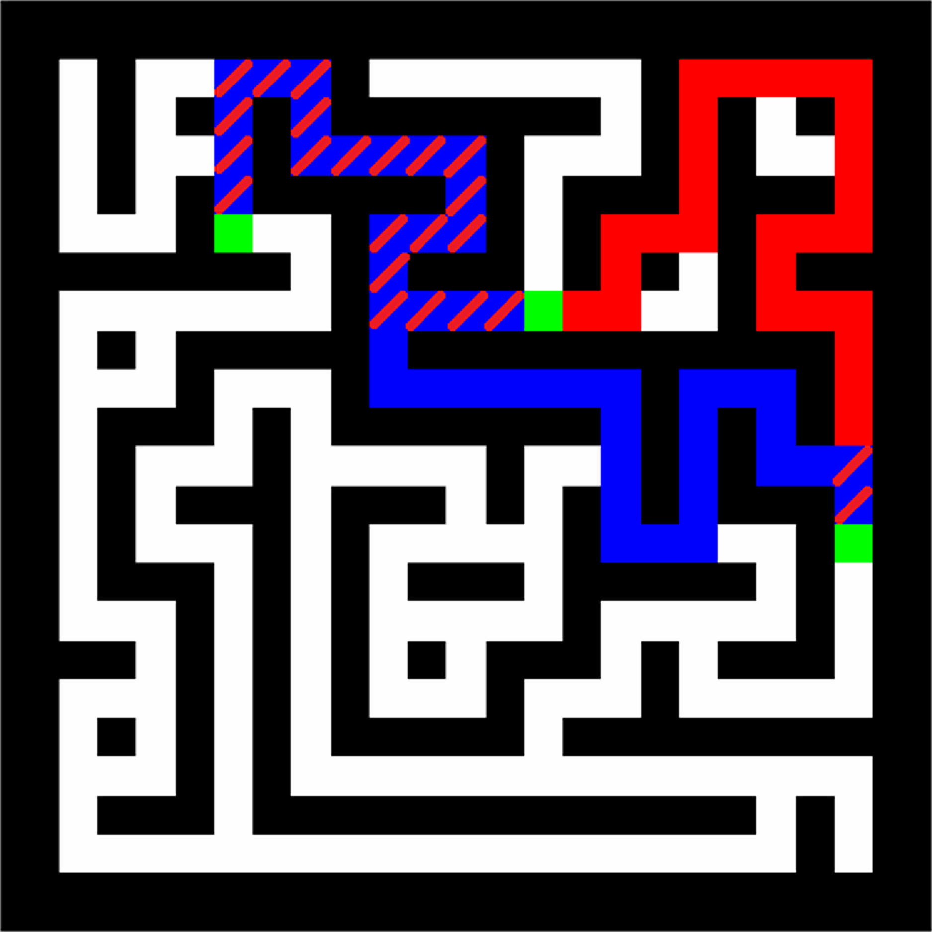

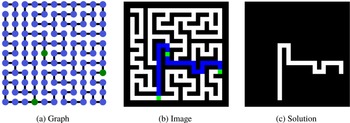

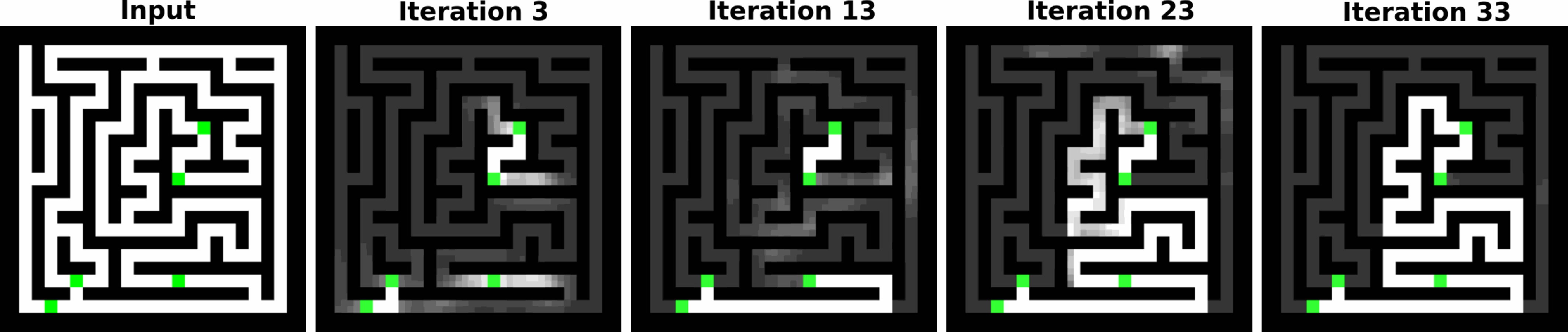
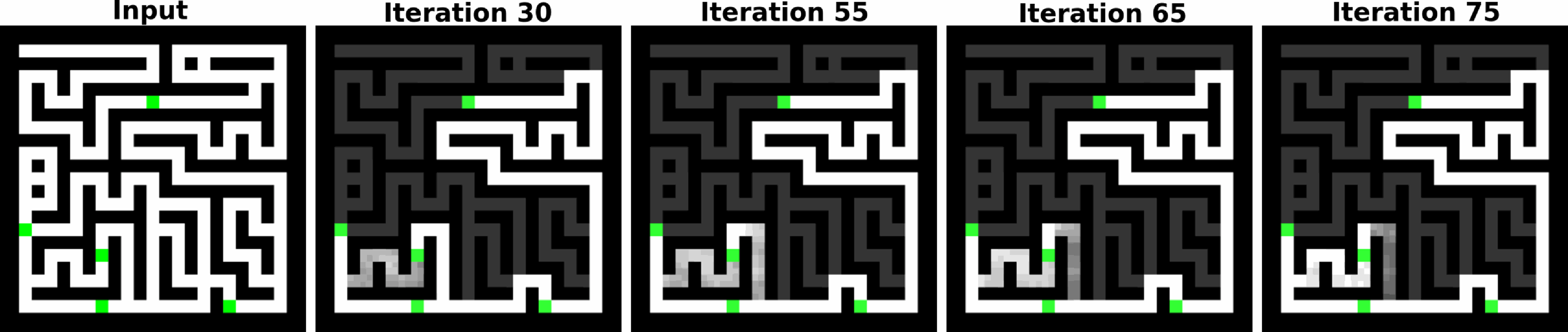
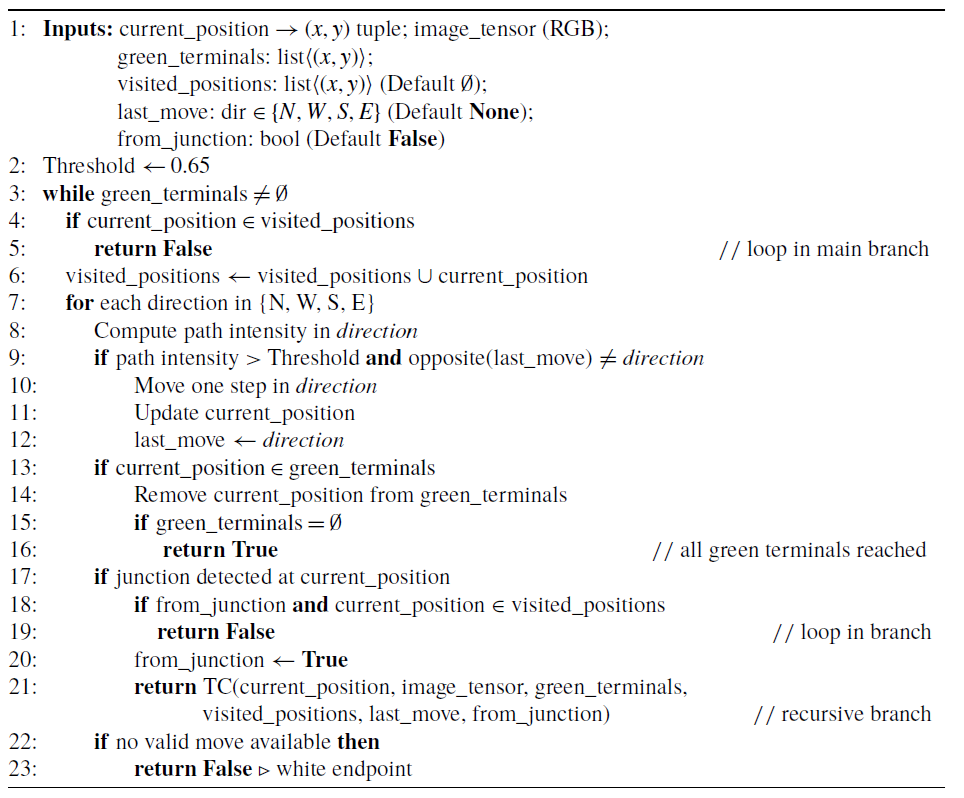
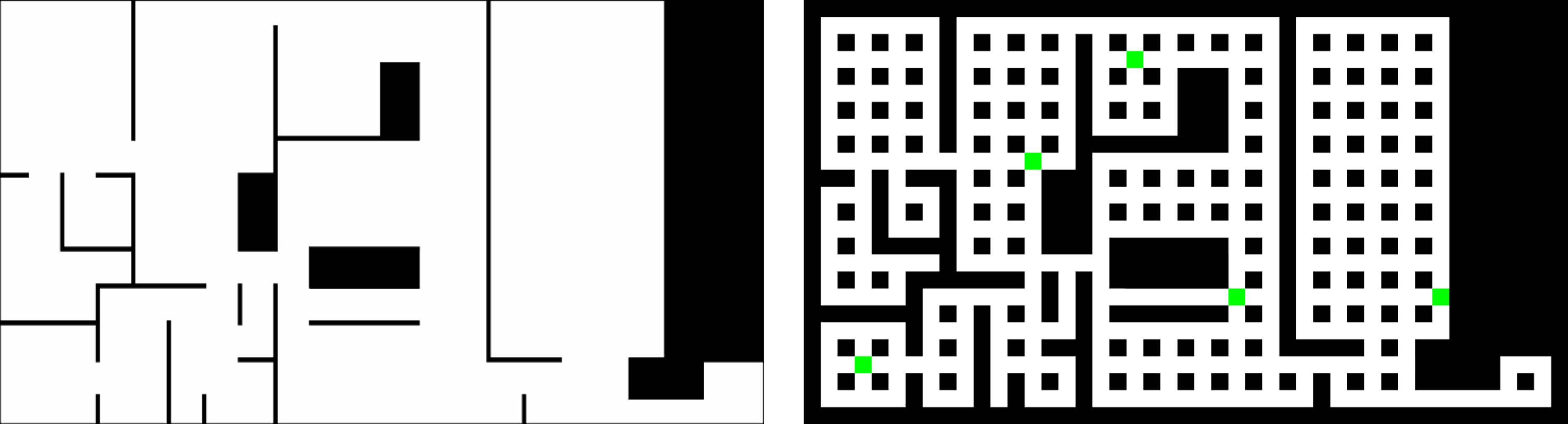
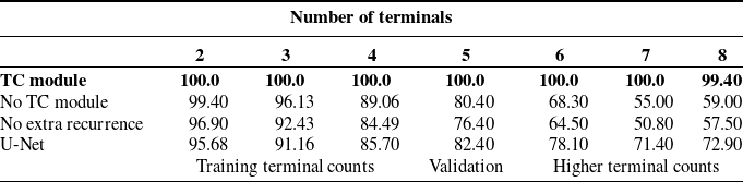
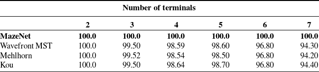
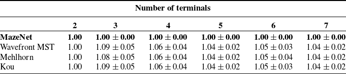
 ±
 >


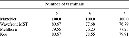
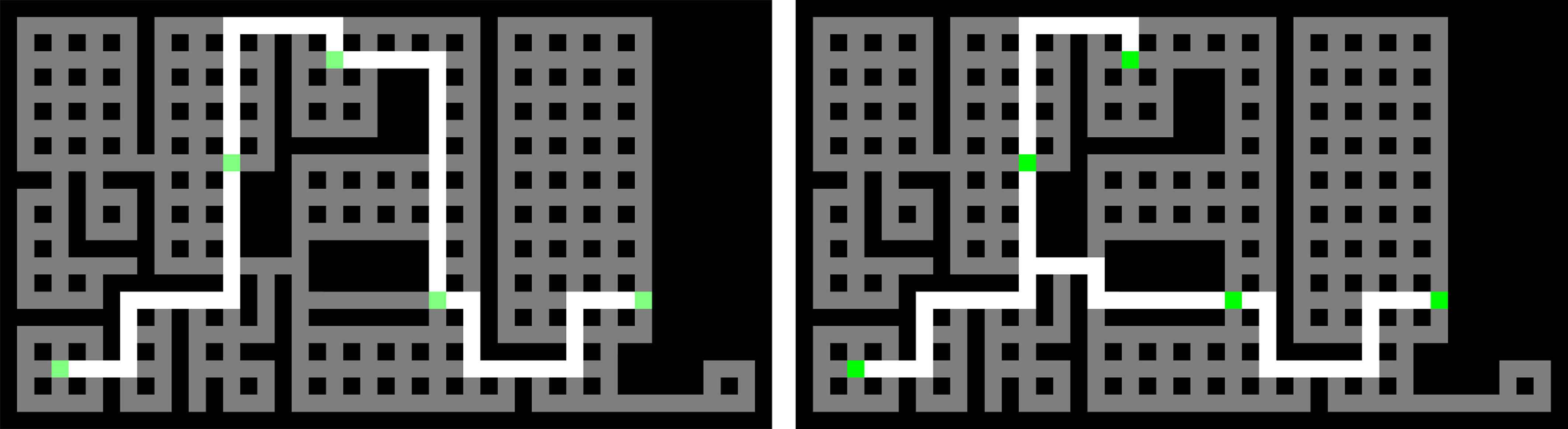

 ±

 ±
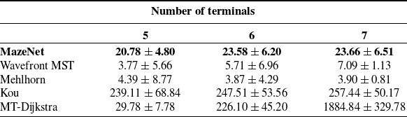
 ±

 ±


 ×

 N=3


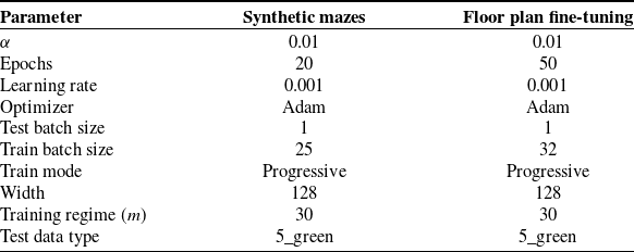


 1000×1000

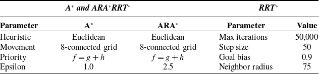

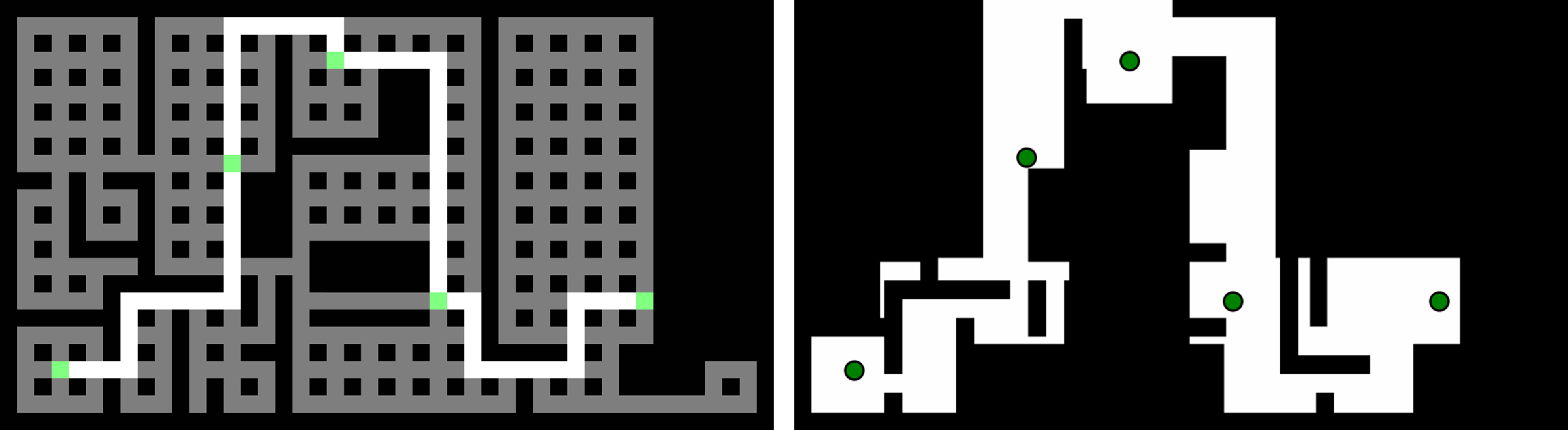
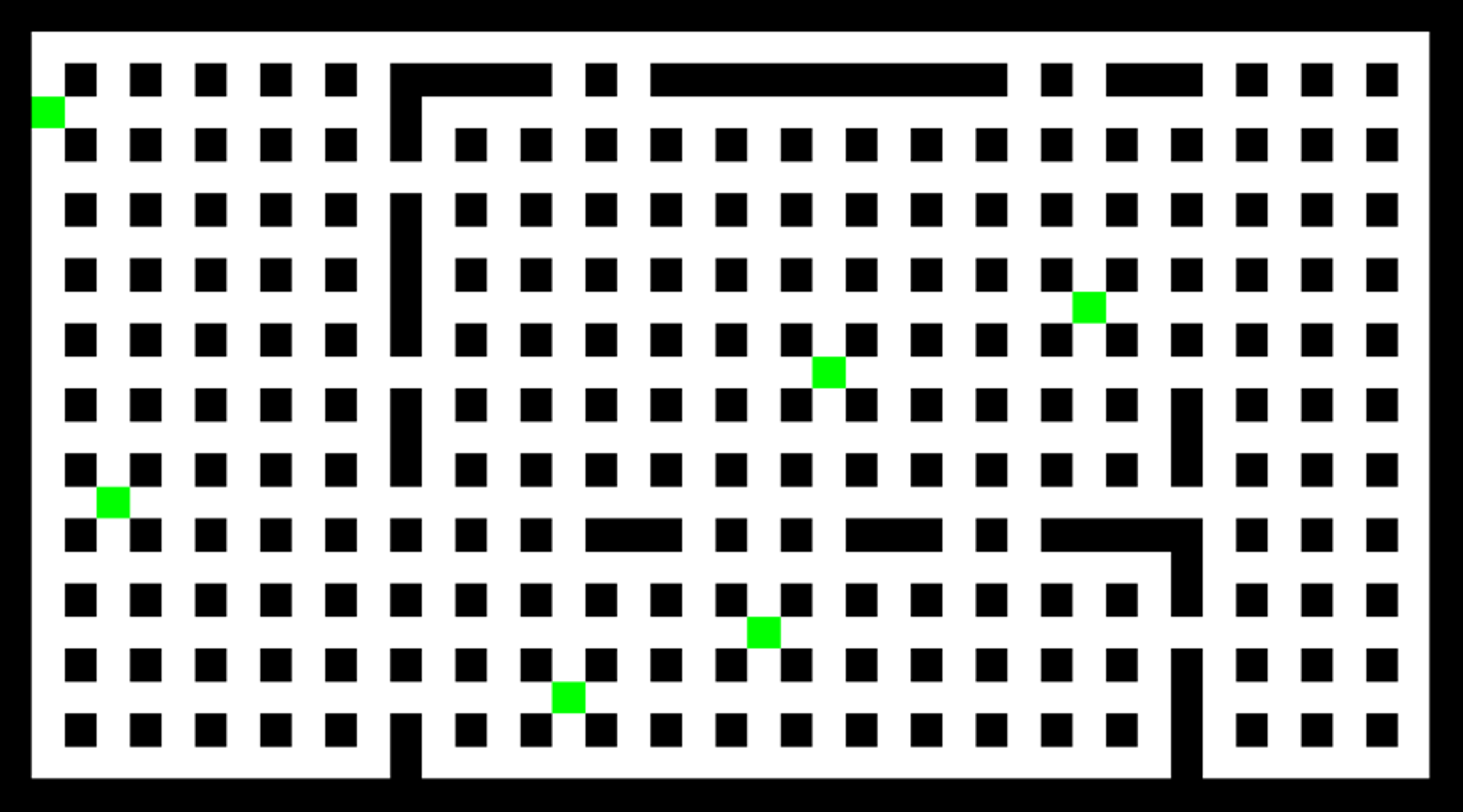
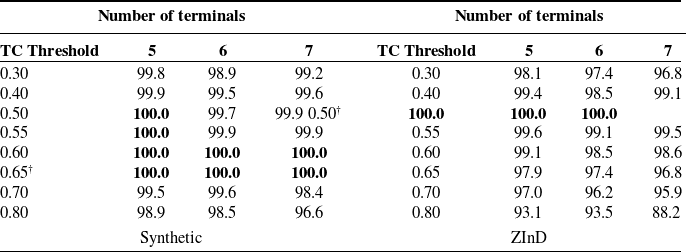
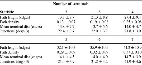
 ±
 ∈[0,1]
 ≥3
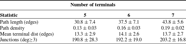
 ±
 ∈[0,1]
 ≥3
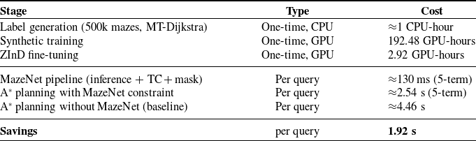
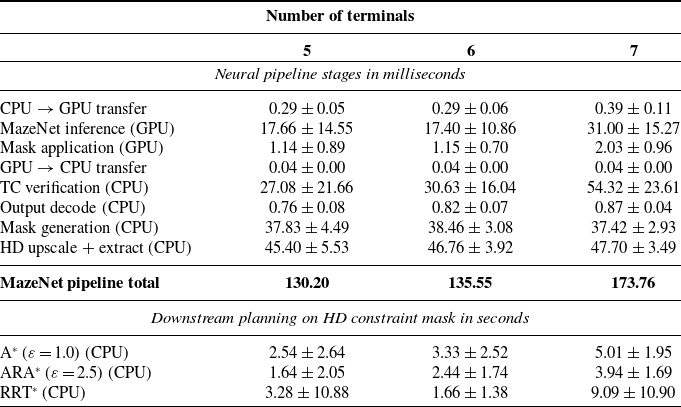
 ±
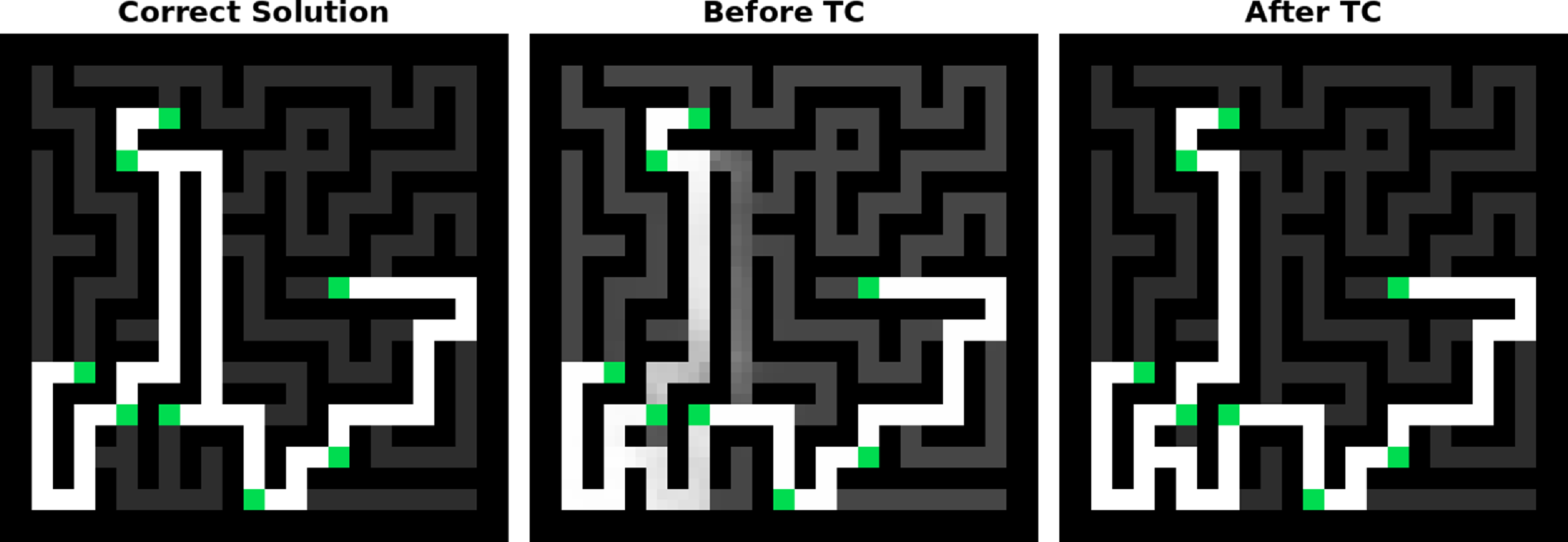
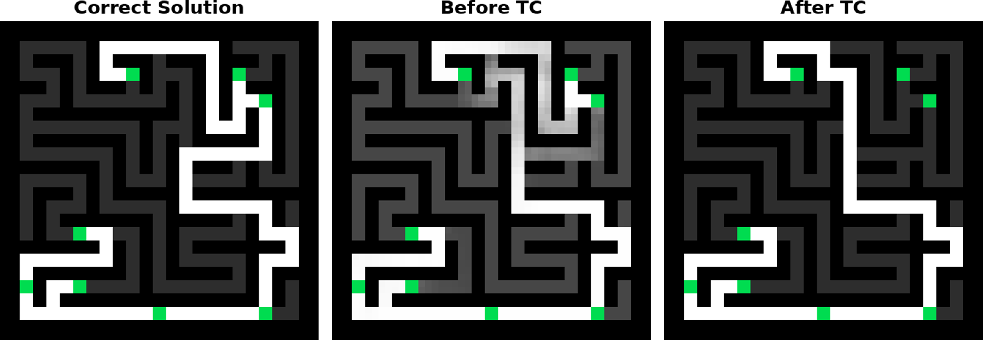


 Open access

