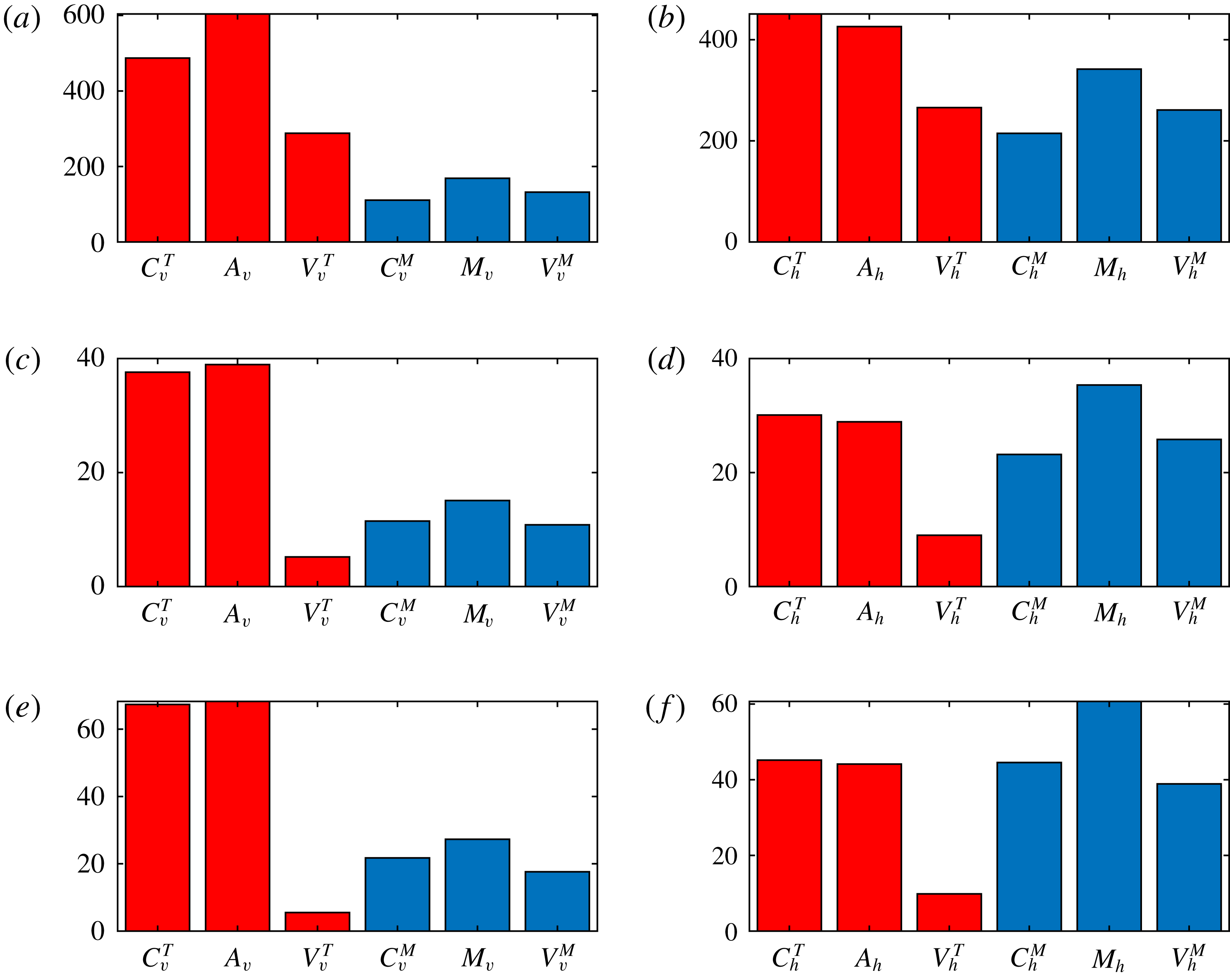
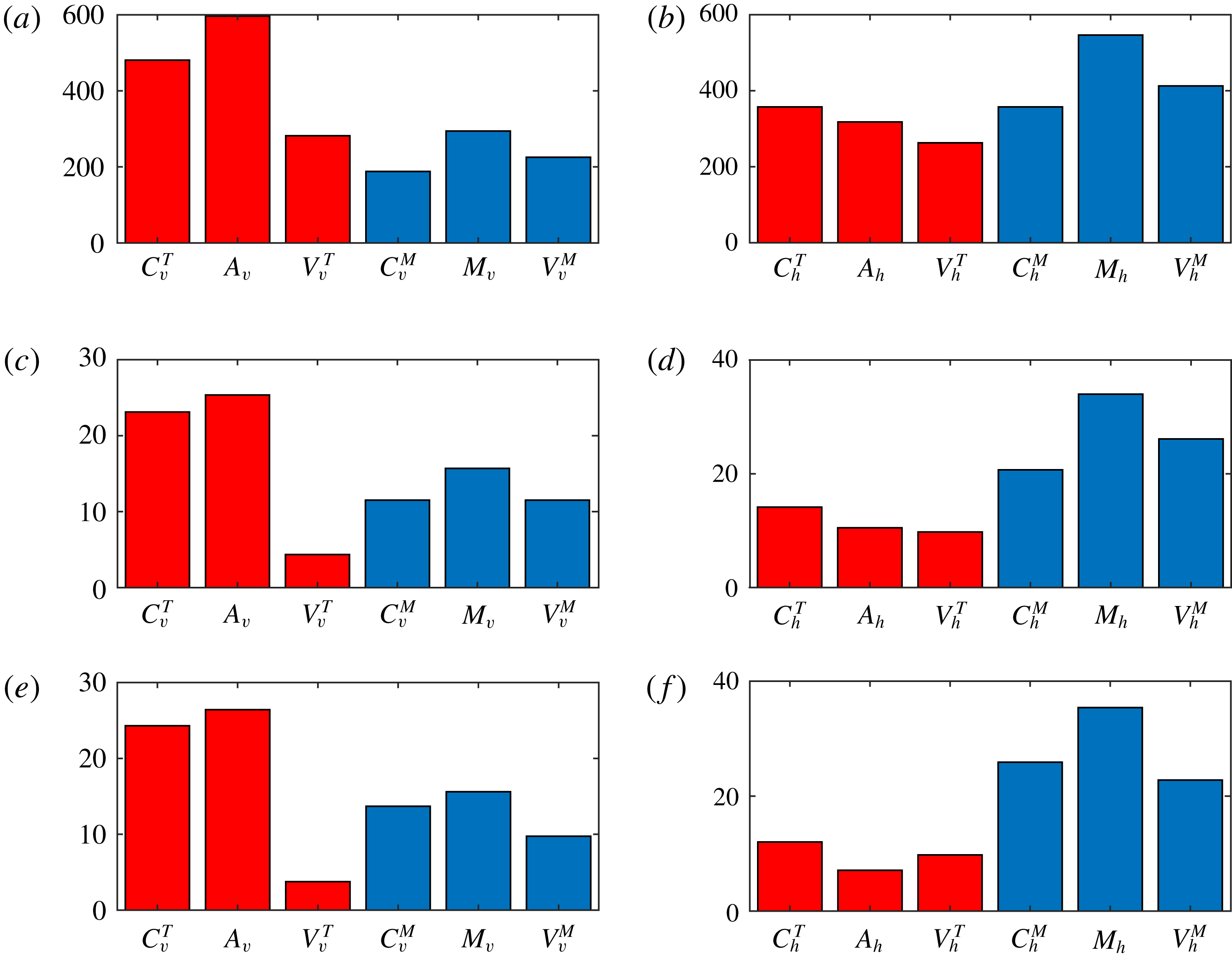
1 Introduction
In rapidly rotating convection, the Coriolis force strongly constrains the dynamics. For example, in the Earth’s liquid outer core, the convective overturning time is of the order of a century, whereas the rotational period is, by definition, one day. The Coriolis force can then balance any residual force acting on the fluid so efficiently that the inertia terms in the momentum equation (i.e. the advective derivative of the velocity) can be neglected. Thus, at small values of the Rossby number (the ratio of rotational to convective time scales), the fluid behaves as if it has no inertia. In such systems, magnetic fields can then play a crucial role in the dynamics since the Lorentz force can circumvent some of the rotational constraints. These issues are important in cases when the magnetic field is externally imposed, as is the case in magnetoconvection (e.g. Chandrasekhar Reference Chandrasekhar1961; Eltayeb & Roberts Reference Eltayeb and Roberts1970; Eltayeb Reference Eltayeb1972), but can become central in convectively driven dynamos, where both the flow and magnetic field have to be maintained self-consistently (e.g. Roberts Reference Roberts, Roberts and Soward1978; Roberts & Soward Reference Roberts and Soward1992).
First steps towards understanding the generation of magnetic fields in rapidly rotating convection, neglecting inertia, were taken by Jones & Roberts (Reference Jones and Roberts2000), who considered a plane layer model of Boussinesq convection (see also Rotvig & Jones Reference Rotvig and Jones2002). A similar model was analysed by Hughes & Cattaneo (Reference Hughes and Cattaneo2016), who considered the geophysical implications, and, in more detail, by Cattaneo & Hughes (Reference Cattaneo and Hughes2017) (hereinafter Paper 1). The crucial feature of these latter studies was to note that in a system with no inertia, the momentum equation becomes linear in the velocity, thus permitting a decomposition into thermal and magnetic components. The thermal part of the velocity is driven by buoyancy forces, whereas the magnetic part is driven by Lorentz forces. It was found that this decomposition is helpful in determining the processes by which dynamos saturate. In particular, depending on the parameters, it was possible to identify weak field solutions, in which the hydromagnetic state is close to the hydrodynamic state, and strong field solutions, in which the hydromagnetic and hydrodynamic states are very different.
In a weak field solution, the Lorentz force has a subtle effect on the convection – sufficient to halt the growth of the field, but with no major changes to the amplitude or scale of the convective flow. On the other hand, in simple terms, the idea behind a strong field solution is that the magnetic field generated is able to relax the rotational constraint, thus allowing the convection to flourish, in turn generating more field, and so on. One can then see how the final state may be very different to that of hydrodynamic convection.
Given these two very different types of dynamo solution, it is natural to speculate that the resulting force balance must be very different. In this paper we explore this issue, using the same model as in Paper 1. In the absence of inertia, the dynamics is governed by Coriolis, buoyancy, magnetic and viscous forces. It has therefore been a question of long-standing interest as to how the forces balance. For example, in the absence of magnetic field, the terms in the momentum equation inescapably lead to a balance between viscous, buoyancy (Archimedean) and Coriolis forces (the so-called VAC regime). This leads to the well-known feature that the horizontal scale of the convection decreases as the rotational influence increases. However, once the magnetic field comes into play, via dynamo action, more possibilities arise. In particular, whereas the effect of viscosity is unavoidable in purely hydrodynamic convection, there may be circumstances in the hydromagnetic case in which viscous forces become a minor player; these solutions, if they exist, are referred to as MAC. With such a force balance, would convection then be able to develop on larger scales? Alternatively, even in the presence of strong magnetic fields, viscous forces may always remain significant. In such a dynamo, what then determines the scale of the convection?
The role of viscous stresses is often discussed in terms of Taylor’s constraint (Taylor Reference Taylor1963), and how close a given dynamo solution is to satisfying it. In inertialess inviscid systems – with neither inertia nor viscosity able to take up the slack – the question of force balance is particularly acute. In spherical geometry, this leads to Taylor’s constraint, which states that the integrated magnetic torque on any cylindrical surface must vanish; the physical interpretation is that in a system with no inertia and no viscosity, any residual torque would lead to an unimpeded spin-up. In plane layer geometry, as we consider here, the mathematical form of Taylor’s constraint is slightly different, but its physical interpretation in terms of no residual torque remains unchanged. Such Taylor solutions are not easy to find but, if they exist, they describe a dynamo with a strong large-scale field. Is it though possible to find solutions with a strong large-scale field that do not satisfy Taylor’s constraint, i.e. solutions for which viscosity simply cannot be neglected? And what of the weak and strong field solutions identified in Paper 1? How do they fit into this dynamical landscape? Our aim in this paper is to clarify some of these issues by exploring the relation between force balance and properties of the dynamo solutions.
Section 2 contains the mathematical formulation of the dynamo problem, and also reintroduces the decomposition of the velocity into its thermal and magnetic components. Also, for comparison, we introduce the thermo-kinematic approximation, in which the temperature is advected solely by the thermal velocity. In § 3 we describe the procedure by which we compare the forces in the momentum equation. This is a little more complicated than simply looking at the terms in the primitive equation, because of the role of the pressure. Here we introduce the novel approach of projecting the forces onto their solenoidal component. In § 4 we briefly review the properties of the different types of dynamo solutions. Section 5 contains the bulk of the paper, involving a detailed analysis of the different force balances from the different types of dynamo solution. It also describes a comparison of the force balance in the full system with that resulting from the thermo-kinematic approximation. A discussion and concluding remarks are contained in § 6.
2 Mathematical formulation
We consider thermally driven convection in the Boussinesq approximation of a three-dimensional, Cartesian layer of fluid rotating about the vertical. The fluid layer has depth
 $d$
, angular velocity
 $\unicode[STIX]{x1D6FA}$
, density
 $\unicode[STIX]{x1D70C}$
, kinematic viscosity
 $\unicode[STIX]{x1D708}$
, thermal diffusivity
 $\unicode[STIX]{x1D705}$
and magnetic diffusivity
 $\unicode[STIX]{x1D702}$
, all constant. Following standard practice, we adopt the layer depth
 $d$
, the thermal relaxation time
 $d^{2}/\unicode[STIX]{x1D705}$
and the temperature drop across the layer
 $\unicode[STIX]{x0394}T$
as the units of length, time and temperature respectively. We scale magnetic field intensities with
 $(2\unicode[STIX]{x1D6FA}\unicode[STIX]{x1D705}\unicode[STIX]{x1D707}_{0}\unicode[STIX]{x1D70C})^{1/2}$
, where
 $\unicode[STIX]{x1D707}_{0}$
is the magnetic permeability of the medium. With these units, and in standard notation, the evolution equations for a fluid with negligible inertia terms read
 $$\begin{eqnarray}\displaystyle & \displaystyle \boldsymbol{e}_{z}\times \boldsymbol{u}=-\unicode[STIX]{x1D735}p+\boldsymbol{J}\times \boldsymbol{B}+R\,\unicode[STIX]{x1D703}\boldsymbol{e}_{z}+E\unicode[STIX]{x1D6FB}^{2}\boldsymbol{u}, & \displaystyle\end{eqnarray}$$
 $$\begin{eqnarray}\displaystyle & \displaystyle (\unicode[STIX]{x2202}_{t}-q^{-1}\unicode[STIX]{x1D6FB}^{2})\boldsymbol{B}+\boldsymbol{u}\boldsymbol{\cdot }\unicode[STIX]{x1D735}\boldsymbol{B}=\boldsymbol{B}\boldsymbol{\cdot }\unicode[STIX]{x1D735}\boldsymbol{u}, & \displaystyle\end{eqnarray}$$
 $$\begin{eqnarray}\displaystyle & \displaystyle (\unicode[STIX]{x2202}_{t}-\unicode[STIX]{x1D6FB}^{2})\unicode[STIX]{x1D703}+\boldsymbol{u}\boldsymbol{\cdot }\unicode[STIX]{x1D735}\unicode[STIX]{x1D703}=w, & \displaystyle\end{eqnarray}$$
 $$\begin{eqnarray}\displaystyle & \displaystyle \unicode[STIX]{x1D735}\boldsymbol{\cdot }\boldsymbol{B}=\unicode[STIX]{x1D735}\boldsymbol{\cdot }\boldsymbol{u}=0, & \displaystyle\end{eqnarray}$$
where
 $\boldsymbol{J}=\unicode[STIX]{x1D735}\times \boldsymbol{B}$
is the current density,
 $\unicode[STIX]{x1D703}$
denotes the temperature fluctuations relative to a linear background profile, and the velocity
 $\boldsymbol{u}=(u,v,w)$
. Three dimensionless numbers appear explicitly: the rotational Rayleigh number
 $R$
, the Ekman number
 $E$
and the Roberts number
 $q$
; these are defined by
 $$\begin{eqnarray}\displaystyle & \displaystyle R=\frac{g\unicode[STIX]{x1D6FC}\unicode[STIX]{x0394}Td}{2\unicode[STIX]{x1D6FA}\unicode[STIX]{x1D705}},\quad E=\frac{\unicode[STIX]{x1D708}}{2\unicode[STIX]{x1D6FA}d^{2}},\quad q=\frac{\unicode[STIX]{x1D705}}{\unicode[STIX]{x1D702}}, & \displaystyle\end{eqnarray}$$
where
 $g$
is the gravitational acceleration and
 $\unicode[STIX]{x1D6FC}$
is the coefficient of thermal expansion. With the above standard non-dimensionalisation, the Rossby number
 $Ro$
scales as
 $E/Pr$
, where
 $Pr=\unicode[STIX]{x1D708}/\unicode[STIX]{x1D705}$
is the Prandtl number; thus, formally, at finite values of
 $E$
, infinitesimal values of
 $Ro$
correspond to infinite
 $Pr$
. It is crucial to note, though, that the physical basis for the smallness of the inertia terms (of order
 $Ro$
) stems from the rapid rotation.
As noted in Paper 1, the linearity of (2.1) allows a decomposition of the velocity
 $\boldsymbol{u}$
as
 $$\begin{eqnarray}\displaystyle & \displaystyle \boldsymbol{u}=\boldsymbol{u}_{T}+\boldsymbol{u}_{M}, & \displaystyle\end{eqnarray}$$
where
 $\boldsymbol{u}_{T}$
and
 $\boldsymbol{u}_{M}$
satisfy, respectively, the equations
 $$\begin{eqnarray}\displaystyle & \displaystyle \boldsymbol{e}_{z}\times \boldsymbol{u}_{T}=-\unicode[STIX]{x1D735}p_{T}+R\,\unicode[STIX]{x1D703}\boldsymbol{e}_{z}+E\unicode[STIX]{x1D6FB}^{2}\boldsymbol{u}_{T}, & \displaystyle\end{eqnarray}$$
 $$\begin{eqnarray}\displaystyle & \displaystyle \boldsymbol{e}_{z}\times \boldsymbol{u}_{M}=-\unicode[STIX]{x1D735}p_{M}+\boldsymbol{J}\times \boldsymbol{B}+E\unicode[STIX]{x1D6FB}^{2}\boldsymbol{u}_{M}, & \displaystyle\end{eqnarray}$$
with
 $\unicode[STIX]{x1D735}\boldsymbol{\cdot }\boldsymbol{u}_{T}=\unicode[STIX]{x1D735}\boldsymbol{\cdot }\boldsymbol{u}_{M}=0$
and
 $p=p_{T}+p_{M}$
.
The component
 $\boldsymbol{u}_{T}$
is driven by buoyancy forces, whereas the component
 $\boldsymbol{u}_{M}$
is driven by magnetic forces, with the Coriolis force influencing both components. The velocity
 $\boldsymbol{u}_{T}$
exists even in the absence of magnetic fields, and defines the kinematic problem;
 $\boldsymbol{u}_{M}$
, on the other hand, exists only by virtue of the presence of the magnetic field. One can think of
 $\boldsymbol{u}_{M}$
as the means by which the system reacts to the presence of the magnetic field, leading eventually to the saturation of magnetic field growth. Note that in the saturated regime, the temperature distribution depends on both
 $\boldsymbol{u}_{T}$
and
 $\boldsymbol{u}_{M}$
, via (2.3), and hence
 $\boldsymbol{u}_{T}$
does not remain as the kinematic velocity.
If, however, the buoyancy force were to be prescribed, then
 $\boldsymbol{u}_{T}$
would always be independent of the magnetic field. This slightly simpler system, which we refer to as thermo-kinematic, provides, by comparison, useful insights into the behaviour of the full system. For the thermo-kinematic system, the governing equations (2.1), (2.2) and (2.4) are unchanged; however, the temperature equation (2.3) is replaced by
 $$\begin{eqnarray}\displaystyle & \displaystyle (\unicode[STIX]{x2202}_{t}-\unicode[STIX]{x1D6FB}^{2})\unicode[STIX]{x1D703}+\boldsymbol{u}_{T}\boldsymbol{\cdot }\unicode[STIX]{x1D735}\unicode[STIX]{x1D703}=w_{T}. & \displaystyle\end{eqnarray}$$
We adopt the same boundary conditions for the full and thermo-kinematic problems. In the horizontal directions we assume that all fields are periodic with periodicity
 $\unicode[STIX]{x1D706}$
– the aspect ratio. In the vertical we consider standard illustrative boundary conditions, namely that the boundaries are perfectly conducting, both thermally and electrically, impermeable and stress free. Formally these correspond to
 $$\begin{eqnarray}\displaystyle \unicode[STIX]{x1D703}=w=\unicode[STIX]{x2202}_{z}u=\unicode[STIX]{x2202}_{z}v=B_{z}=\unicode[STIX]{x2202}_{z}B_{x}=\unicode[STIX]{x2202}_{z}B_{y}=0\quad \text{at}~z=0,1. & & \displaystyle\end{eqnarray}$$
We solve equations (2.2)–(2.4) numerically by standard pseudo-spectral methods. Details concerning the numerical methods can be found in Cattaneo, Emonet & Weiss (Reference Cattaneo, Emonet and Weiss2003). The numerical scheme requires at every time step a knowledge of the velocity
 $\boldsymbol{u}$
, which can be computed from the elliptical equation (2.1). The details of how this is performed are contained in appendix A of Paper 1.
3 Force projections
As discussed in the introduction, our chief aim in this paper is to understand the force balance in dynamos driven by rapidly rotating convection. One approach would be to consider the magnitude of the various forces in (2.1) (or, equivalently, (2.7) and (2.8)). The drawback with this approach is that the Coriolis, buoyancy and Lorentz terms are all non-solenoidal, and so have a gradient component; these are accommodated by the pressure gradient, which ensures that the flow remains solenoidal, but of itself is not of dynamical significance. A natural way to proceed (e.g. Dormy Reference Dormy2016) would be to take the curl of (2.1). This, however, introduces an extra derivative, which numerically can cause problems in simulations with high fluid and magnetic Reynolds numbers; indeed, the curl of the Lorentz force can be particularly unpleasant. Another possibility, and the one we adopt here, is to consider the projection of (2.7) and (2.8) onto the subspace of solenoidal vector functions. This takes care of the pressure whilst, importantly, not introducing any additional spatial derivatives. The price to pay though is that the interpretation of projected quantities is a little less intuitive than that of the full (non-projected) forces. In particular, such a projection tends to scramble the directional components; for example, the solenoidal projection of a purely vertical force, such as buoyancy, will have both vertical and horizontal components.
Implementation of this procedure in (2.7) and (2.8) leads to six projected forces, governed by the equations
 $$\begin{eqnarray}\displaystyle & \displaystyle \mathbb{P}(R\,\unicode[STIX]{x1D703}\boldsymbol{e}_{z}-\boldsymbol{e}_{z}\times \boldsymbol{u}_{T})+E\unicode[STIX]{x1D6FB}^{2}\boldsymbol{u}_{T}=0, & \displaystyle\end{eqnarray}$$
 $$\begin{eqnarray}\displaystyle & \displaystyle \mathbb{P}(\boldsymbol{J}\times \boldsymbol{B}-\boldsymbol{e}_{z}\times \boldsymbol{u}_{M})+E\unicode[STIX]{x1D6FB}^{2}\boldsymbol{u}_{M}=0, & \displaystyle\end{eqnarray}$$
where
 $\mathbb{P}$
denotes the solenoidal projection operator. Note that since the viscous terms are already solenoidal, these do not require projection.
We denote the projections of the magnetic, buoyancy, Coriolis and viscous forces by
 $M$
,
 $A$
,
 $C$
and
 $V$
, respectively. Since the system is strongly anisotropic, it is instructive to consider separately the horizontal and vertical components, which we denote by the subscripts
 $h$
and
 $v$
; furthermore, since we are interested in the Coriolis and viscous forces for the thermal and magnetic velocities separately, we introduce the superscripts
 $T$
and
 $M$
for these projections.
4 Dynamo solutions
Our analysis is based on the study of three representative cases. The input parameter values for these are contained in table 1, together with
 $R_{c}$
, the critical Rayleigh number at the onset of convection. We also show
 $Rm$
, the magnetic Reynolds number, and the kinetic and magnetic Taylor microscales, all of which are output parameters. The numerical resolution is the same in all cases; to ensure that all quantities, included diagnostic ones, were fully resolved, we employed a higher resolution than that used in Paper 1. Certain aspects of these solutions have been discussed in Paper 1 and so here we give just a brief summary of their dynamo properties. In all three cases, the convection is vigorously time dependent and supports dynamo action; the essential difference between the three cases is in the manner in which the dynamo saturates. In Paper 1 we introduced the idea of weak and strong field dynamos categorised by the departure of the dynamic from the kinematic velocity. The three cases studied here correspond to a weak field dynamo (case 1, in which, in the decomposition (2.6),
 $\boldsymbol{u}\approx \boldsymbol{u}_{T}$
), a strong field dynamo (case 2, in which both
 $\boldsymbol{u}_{T}$
and
 $\boldsymbol{u}_{M}$
contribute significantly to
 $\boldsymbol{u}$
) and a super strong field dynamo (case 3, in which
 $\boldsymbol{u}\approx \boldsymbol{u}_{M}$
). These three cases are illustrated in figure 1, which shows snapshots of the vertical components of
 $\boldsymbol{u}$
,
 $\boldsymbol{u}_{T}$
and
 $\boldsymbol{u}_{M}$
. As discussed in Paper 1, it is important to make the distinction between weak and strong field branches and what we refer to as weak and strong field solutions. Our nomenclature addresses the issue of the force balance that leads to dynamo saturation rather than the branch on which the solutions lie.
Summary of the parameter values for the simulations. The input parameters are
 $E$
,
 $R$
,
 $q$
and
 $\unicode[STIX]{x1D706}$
.
 $R_{c}$
denotes the critical Rayleigh number for the onset of convection; the magnetic Reynolds number
 $Rm=q\langle \boldsymbol{u}^{2}\rangle ^{1/2}$
, where the root mean square (r.m.s.) velocity is obtained from a time average in the saturated state;
 $l_{v}$
and
 $l_{B}$
denote, respectively, the Taylor microscales for the velocity and the magnetic field, defined by
 $l_{v}^{2}=\langle |\boldsymbol{u}|^{2}\rangle /\langle |\unicode[STIX]{x1D735}\times \boldsymbol{u}|^{2}\rangle$
,
 $l_{B}^{2}=\langle |\boldsymbol{B}|^{2}\rangle /\langle |\unicode[STIX]{x1D735}\times \boldsymbol{B}|^{2}\rangle$
. The resolution for all cases is
 $1024\times 1024\times 257$
.

Snapshots of the vertical components of
 $\boldsymbol{u}$
(a,d,g),
 $\boldsymbol{u}_{T}$
(b,e,h) and
 $\boldsymbol{u}_{M}$
(c,f,i) for case 1 (a–c), case 2 (d–f) and case 3 (g–i) in a horizontal plane near the top of the domain. Each row is scaled consistently. Light (dark) tones correspond to upward (downward) moving fluid.

Historically, a problem of great interest in dynamo theory has been the generation of large-scale (mean) fields by helical convection, through what is referred to as the dynamo
 $\unicode[STIX]{x1D6FC}$
-effect. As expected, the influence of rotation on the convection does indeed introduce helicity into the flow; in Boussinesq convection, the helicity distribution is antisymmetric about the mid-plane (see Paper 1, figure 3). However, in the turbulent regimes studied here, the mean field generated is rather weak, despite the presence of helicity (see Paper 1, figure 10); it is worth noting that the absence of a mean field is not related to the neglect of inertia (see Cattaneo & Hughes Reference Cattaneo and Hughes2006). Thus, whether we are discussing weak or strong field dynamo solutions, they should not be regarded as mean-field-type dynamos.
5 Force balance

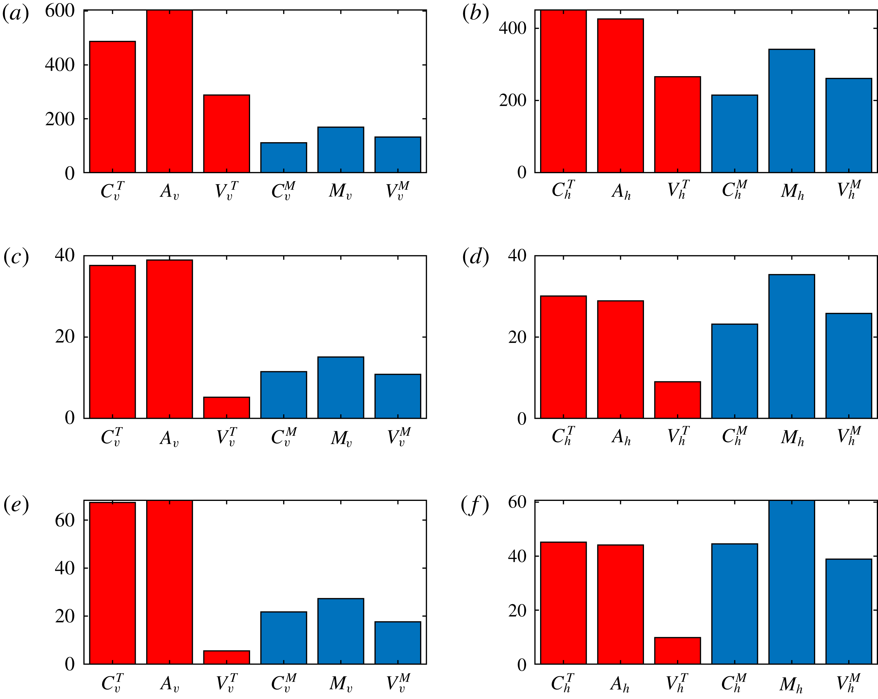
It is clear from inspection of figure 1 that the mechanism of dynamo saturation is very different in the three cases studied. In order to understand how this is achieved, it is necessary to analyse the means by which the exact force balance relations (3.1) and (3.2) are effected. Of course, this analysis must take into account the vectorial nature of the equations, but as a first step we can look at the magnitudes of the forces, separating the horizontal and vertical components of the various terms. Figure 2 plots the magnitudes of the horizontal components of the forces for the particular example of case 2. Two features are apparent. One is that there is a considerable range in the magnitudes of the various forces; the other is that, although there is some temporal variation in the magnitudes, this is small compared to their mean value. This is true for all three cases, for both the vertical and horizontal components. It therefore makes sense to consider the time-averaged quantities of the magnitudes of the forces, in which each term in (3.1) and (3.2) has both vertical and horizontal components. This then leads to a convenient graphical representation for the magnitudes of all of the terms in (3.1) and (3.2) in terms of bar charts.
Figure 3 shows the time-averaged r.m.s. values of the vertical and horizontal components of all six projected forces in (3.1) and (3.2), for all three cases studied. Several salient features are evident. In terms of the thermal force balance (3.1), the Coriolis and buoyancy forces dominate, in both the vertical and horizontal projections; indeed, in the progression from weak to strong to super strong solutions, the Coriolis and buoyancy forces become more and more balanced (i.e.
 $C_{v/h}^{T}\approx A_{v/h}$
). For the magnetic force balance (3.2), the horizontal projections dominate for all three forces in all three cases. In the horizontal projections for the weak field solutions, all six forces are of comparable magnitude. In progressing to the strong and then super strong field solutions, the magnetic tension (
 $M_{h}$
) becomes dominant, with the thermal viscous stresses (
 $V_{h}^{T}$
) becoming progressively smaller; this trend for the diminishing of the thermal viscous stresses is also apparent in the vertical projections. Thus, as noted above, as one progresses from weak to super strong, there is a tendency in the thermal force balance equation for equality between Coriolis and buoyancy forces, with viscosity becoming irrelevant. This should be contrasted with the magnetic force balance equation, in which no such tendency is observed, with the viscous term (
 $V_{v/h}^{M}$
) always remaining important. This last result has some interesting implications for the role of viscous stresses in determining the nature of the solutions. For instance, if the solution approaches a Taylor state, with an exact balance between Coriolis, buoyancy and magnetic forces, then the viscous stresses would become irrelevant. Here, although the viscous stresses associated with the thermal component of the velocity (
 $V_{v/h}^{T}$
) do become small, this is not the case for those associated with the magnetic component (
 $V_{v/h}^{M}$
). If that is true in general, then this system does not have a tendency to approach a Taylor state; all three terms in (3.2) remain of comparable magnitude.
Vertical components of the projections of the Coriolis (a,c) and buoyancy (b,d) terms in the thermal force balance equation (3.1), for case 1 (a,b) and case 2 (c,d), in a horizontal plane near the top of the domain. Each row is scaled consistently. Light (dark) tones correspond to positive (negative) values.

Horizontal components of the projections of the Coriolis (a,c) and magnetic (b,d) terms in the magnetic force balance equation (3.2), for case 1 (a,b) and case 2 (c,d), in a horizontal plane near the top of the domain. Each row is scaled consistently. Light (dark) tones correspond to positive (negative) values.

Enlargement of a
 $\unicode[STIX]{x1D706}/4\times \unicode[STIX]{x1D706}/4$
section of figure 5 for case 2.

In order to gain some insight into the role of viscous stresses, it is useful to inspect the spatial distribution of the terms in (3.1) and (3.2). First we look at the vertical components of the thermal force balance equation (3.1). Figure 4 shows the horizontal planform, near the upper boundary, of the Coriolis and buoyancy terms for cases 1 and 2. Just as a reminder, it should be noted that for case 1, the aspect ratio is
 $\unicode[STIX]{x1D706}=5$
, whereas for case 2,
 $\unicode[STIX]{x1D706}=2$
. The Coriolis term is smoother than the corresponding buoyancy term, with the difference between them being accommodated by the viscous term. Clearly the difference between the two is reduced in the strong field solution. Indeed, this trend continues into the super strong regime, and it is conceivable that there will be regimes in which the Coriolis and buoyancy forces are arbitrarily close. This should be contrasted with the horizontal components of the magnetic force balance equation (3.2), shown in figure 5. Clearly the magnetic tension has a smooth component that can be balanced by the Coriolis term, but it also has a strongly intermittent, filamentary part that can be accommodated only by the viscous stresses; this can be seen particularly clearly in the blow-up of part of the domain shown in figure 6. The important feature is that this latter component does not appear to become any weaker in the progression from weak to strong field solutions. This intermittent component of the magnetic stresses is associated with current sheets, and there is no evidence here that these will ever disappear.
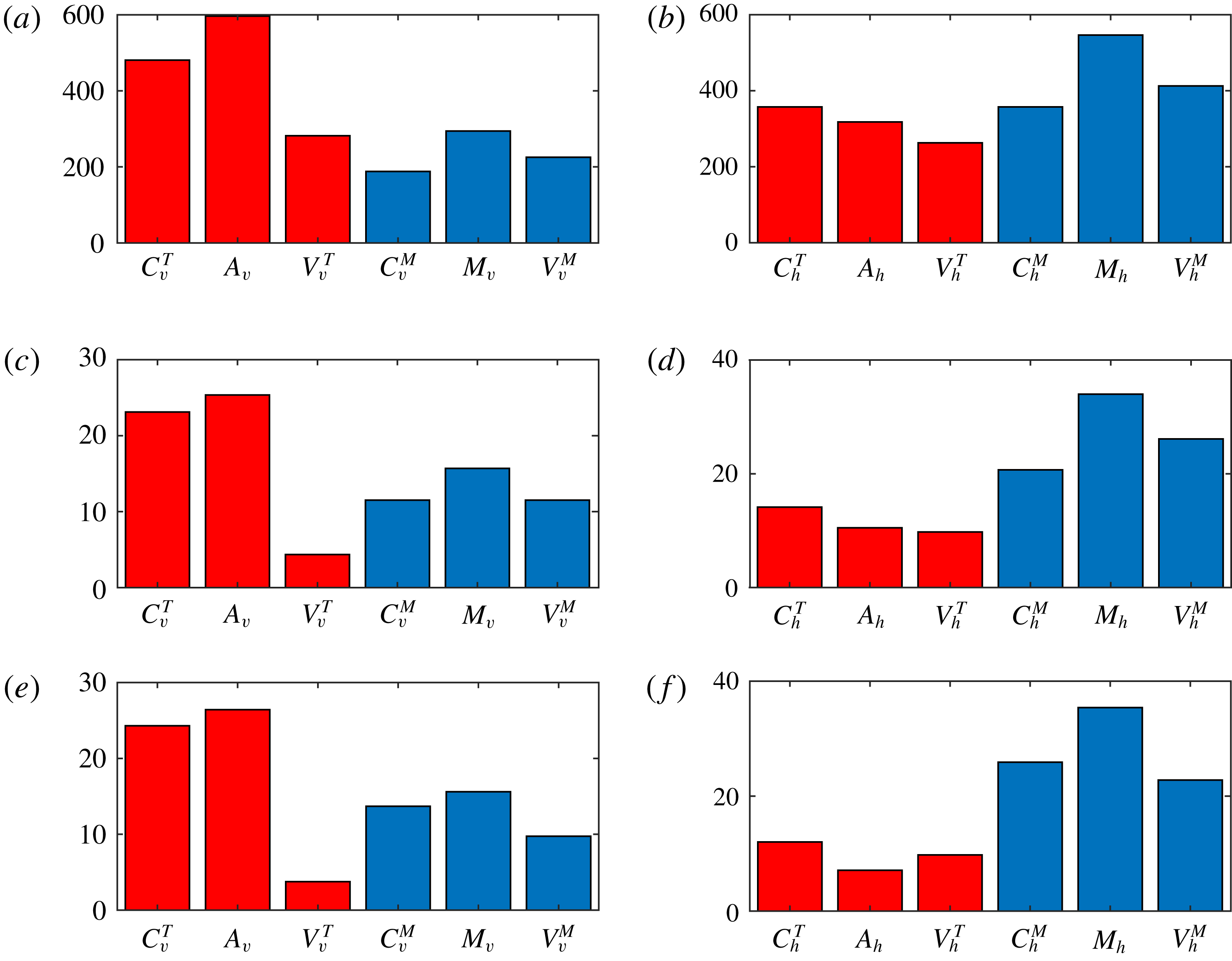
Further insight into the underlying physical processes can be gained from consideration of the thermo-kinematic problem, described in § 2. The key difference between the full and thermo-kinematic systems is that in the former the temperature is advected by the full velocity, and hence is influenced by the magnetic field, whereas in the latter, by construction, the temperature is what it would be in unmagnetised convection. In the full problem, the role of magnetic forces is twofold: to generate counter-vorticity and also to change the planform of convection, typically increasing its scale. In weak field solutions, this increase is only slight, whereas in strong field solutions it is substantial. By contrast, in the thermo-kinematic problem, in which the convective planform is fixed, there is only one route to saturation, namely the Lorentz force can only generate counter-vorticity.
Figure 7 shows the quantities corresponding to those in figure 3 for the thermo-kinematic problem with the same parameter values as cases 1 to 3. The magnitudes of the components in the magnetic force balance (3.2) are very similar to the corresponding quantities in the full problem. This is not surprising, since the magnetic part of the problem is unchanged. For the limiting case of a weak solution, the thermal forces in the full and thermo-kinematic problems will be identical, since that is precisely the definition of a weak solution. In our weak solution (case 1), there is however some weak coupling between the thermal forces and the magnetic field, which allows the dynamo to saturate at a lower level in comparison with the thermo-kinematic problem. For cases 2 and 3, the most striking difference is in the vertical components of the thermal forces, where the amplitude of the thermal forces is reduced relative both to those of the full system and also to the magnetic terms. This reduction in amplitude illustrates the vital role of the magnetic field in alleviating rotational constraints. For purely hydrodynamic convection, the rotational constraint manifests itself in a dependence of the horizontal scale of convection as
 $E^{1/3}$
for
 $E\ll 1$
; this follows from the thermal force balance equation (2.7) and the temperature equation (2.3), which are precisely the thermo-kinematic equations. However, there is no such equivalent relationship deriving from the magnetic force balance equation (2.8) together with the induction equation (2.2). That being the case, for small
 $E$
, both the thermal velocity
 $\boldsymbol{u}_{T}$
and the temperature
 $\unicode[STIX]{x1D703}$
in the thermo-kinematic system can only be at small scales, whereas
 $\boldsymbol{u}_{M}$
can have, and indeed does have, a large-scale component. By contrast, in the full system, the presence of the large-scale
 $\boldsymbol{u}_{M}$
in the temperature equation (2.3) introduces a large-scale component in the temperature and therefore in the buoyancy force, which drives
 $\boldsymbol{u}_{T}$
towards larger scales. Thus the rotational constraint is released and the thermal velocity can attain larger amplitudes.
Time-averaged convective flux
 $\langle w\unicode[STIX]{x1D703}\rangle$
versus depth for case 2, with its constituent components
 $\langle w_{T}\unicode[STIX]{x1D703}\rangle$
and
 $\langle w_{M}\unicode[STIX]{x1D703}\rangle$
. Also shown is the convective flux
 $\langle w\unicode[STIX]{x1D703}\rangle _{tk}$
for the purely hydrodynamic (thermo-kinematic) case.

A particularly striking consequence of this effect is in the increased efficiency of the convection; this can be measured by the convective flux
 $F_{c}=\langle w\unicode[STIX]{x1D703}\rangle$
, where the average is taken over horizontal planes. For example, figure 8 shows the depth dependence, for case 2, of the time-averaged convective flux associated with the thermal velocity
 $w_{T}$
, the magnetic velocity
 $w_{M}$
and the full velocity
 $w$
(the sum of the two). We also show
 $F_{c}$
for the corresponding thermo-kinematic case, equivalent to purely hydrodynamic convection. Of note is the striking increase in convective efficiency in the magnetic system. Although the contribution to the heat transport from the thermal velocity has dropped slightly, this is more than compensated by the contribution from the induced magnetic velocity
 $\boldsymbol{u}_{M}$
, a fact that, in itself, is far from obvious. Thus, in rapidly rotating systems, hydromagnetic convection is considerably more efficient than its hydrodynamic counterpart, in contrast to non-rotating convection in which the influence of magnetic field is inhibiting (e.g. Cattaneo Reference Cattaneo1999).
6 Discussion
In this paper, we have studied dynamo action in rotating, plane layer Boussinesq convection in the absence of inertia. Having found different families of dynamo solutions in Paper 1 (weak, strong and super strong), here we extend this work to analyse the resulting force balance in the saturated dynamo states. By exploiting the linearity of the momentum equation in the inertialess regime, which allows a decomposition of the velocity into thermal and magnetic components, we are able to provide a detailed breakdown of the various contributions to the overall dynamics. For comparison, we also study a thermo-kinematic system, in which the temperature evolves under the influence of the thermal (rather than the full) velocity. The force balance analysis is carried out by extracting the solenoidal component of the momentum equation and then comparing the various terms, decomposed into their horizontal and vertical components.
The reason why we choose to compare the solenoidal component of the forces, rather than the forces themselves, is related to the role of the pressure. It could be argued that in a rapidly rotating system, the leading-order balance is, for example, between the Coriolis force and the pressure gradient. However, in incompressible fluid dynamics, the role of the pressure is to ensure that the flow remains solenoidal; indeed, this is made clear in a variational formulation of the equations of incompressible fluid dynamics, where the pressure
 $p$
appears as a Lagrange multiplier associated with the constraint
 $\unicode[STIX]{x1D735}\boldsymbol{\cdot }\boldsymbol{u}=0$
. In general, although the individual terms in the momentum equation can have a large irrotational component, these parts are then taken care of by the pressure; thus they do not contribute to the motion of the fluid, but they can obscure the analysis of the force balance. The natural way to proceed therefore is to take the curl of the momentum equation, thus eliminating the pressure. This is a perfectly acceptable course of action, since in the resulting equation for the vorticity there is no loss of information. The reason we chose not to follow this approach here was thus not mathematical but numerical, since the extra derivative involved in taking the curl can be difficult to control. Instead we employ the solenoidal projection operator, which removes the irrotational components without introducing a further derivative.
On applying this projection technique to three types of dynamo solution, we find some definite trends. One is that the (projected) magnetic forces are sub-dominant in the vertical direction, but are a significant player in the horizontal direction, becoming the dominant force in the strong and super strong solutions. Thus we conjecture that for this model it is the horizontal dynamics that is responsible for the saturation of the dynamo. In the thermal velocity equation (3.1), in going from weak to strong to super strong solutions, the viscous terms become less and less important, in both the vertical and horizontal directions. This is due to the thermal velocity moving to larger scales, with a resulting balance between Coriolis and buoyancy forces. Interestingly, this is never the case for the magnetic velocity equation (3.2). We find no evidence that the viscous stresses associated with the magnetic velocity become small: the force balance in (3.2) always involves all three terms.
How do these solutions fit into the general scheme of weak and strong solutions? Clearly it cannot be argued that even the strong and super strong field solutions are MAC, since the viscous term associated with the magnetic velocity is always significant. Thus, if anything, such solutions could be described as
 $\text{V}^{M}\text{MAC}$
, rather than the full VMAC. To see why the viscous stresses associated with
 $\boldsymbol{u}_{T}$
can be neglected, but not those associated with
 $\boldsymbol{u}_{M}$
, it is instructive to consider figures 4 and 5. The Coriolis and buoyancy forces associated with the thermal velocity are smooth and, for the strong field solution, almost comparable, leaving little residue for the viscous term to accommodate. By contrast, although the Coriolis term associated with the magnetic velocity is still smooth, the magnetic tension is dominated by sharp filamentary structures, arising from the Lorentz force, which is not only quadratic but involves a derivative of the magnetic field. The inevitable mis-match between these two will always have small-scale structures, thus rendering the viscous term essential. The foregoing conclusion of course rests on the assumption that the scale of viscous dissipation is greater than that of magnetic dissipation, which is definitely the case here. On the other hand, if Ohmic dissipation is sufficiently effective, then the Lorentz force may possess the same degree of smoothness as the Coriolis force.
The above considerations may have implications for finding solutions that are in MAC balance – also known as Taylor states. In such a Taylor solution, in which viscosity is neglected, the projected Lorentz force cannot have small-scale filamentary features. Suppose now that a small-scale perturbation to a Taylor state is introduced in the magnetic field. This would generate a sharp small-scale feature in the Lorentz force; this, in turn, would drive a small-scale magnetic velocity which, through the induction equation, would generate an even smaller-scale magnetic field. With no viscous dissipation to control this process, it is conceivable that the outcome is to drive the dynamics away from the Taylor manifold, assuming of course that the Ohmic dissipation is sufficiently small. Thus the implication here is that, in this regime, Taylor solutions, even when they exist, may be unstable, and turn into something like the strong (and super strong) solutions exhibited here, in which the magnetic field drives the flow towards both large and small scales. On the other hand, if a stable MAC solution exists then it cannot be connected to any kinematic dynamo: if Ohmic dissipation is sufficiently large to inhibit the creation of small scales then it will also prevent kinematic dynamo action at those scales. Thus the only way to find a MAC solution numerically – apart from a very fortunate choice of initial conditions – is first to latch onto a strong
 $\text{V}^{M}\text{MAC}$
solution, by being above the threshold for dynamo action, and then to increase the Ohmic dissipation or reduce
 $E$
in the hope that this nonlinear solution persists. This is the strategy pursued by several groups studying dynamo action in rotating spherical shells, in which the long-term objective is to obtain MAC solutions to model the Earth’s dynamo. Despite the enormous computational difficulties, there has been considerable progress and the latest simulations show promising progress towards these MAC states (e.g. Yadav et al.
Reference Yadav, Gastine, Christensen, Wolk and Poppenhaeger2016; Aubert, Gastine & Fournier Reference Aubert, Gastine and Fournier2017; Schaeffer et al.
Reference Schaeffer, Jault, Nataf and Fournier2017). It will be of interest to pursue this question in the inertialess model studied here.
Acknowledgements
This research was supported in part by STFC grant ST/N000765/1. The computations were undertaken on ARC1 and ARC2, part of the High Performance Computing facilities at the University of Leeds, and also on the COSMA Data Centric system at Durham University, operated by the Institute for Computational Cosmology on behalf of the STFC DiRAC HPC Facility (www.dirac.ac.uk). This equipment was funded by a BIS National E-infrastructure capital grant ST/K00042X/1, DiRAC Operations grant ST/K003267/1 and Durham University. DiRAC is part of the National E-Infrastructure.