1 Introduction
The Marangoni effect, named after the Italian physicist Carlo Marangoni, refers to mass transfer along the interface between two fluids arising from variations in surface tension. These variations are typically caused by gradients in solute/surfactant concentration, or temperature along the interface. When a concentration gradient is responsible for the variation in surface tension, the Marangoni effect is known as the solutocapillary effect, whereas when a temperature gradient drives the surface tension variation, then the Marangoni effect is referred to as the thermocapillary effect. In situations where both gradients are present, the solutocapillary and thermocapillary effects occur simultaneously. In this paper we study these competing effects by considering a thin liquid layer that is doped with a soluble surfactant and allowed to flow down an incline that is maintained at a higher temperature than that of the ambient surroundings. The initial experiments of Kapitza & Kapitza (Reference Kapitza and Kapitza1949) and the subsequent theoretical investigations of Benjamin (Reference Benjamin1957) and Yih (Reference Yih1963) have clearly demonstrated that an isothermal, surfactant-free, gravity-driven flow will become unstable provided that  $Re>5\cot \unicode[STIX]{x1D6FD}/6$ where
 $Re$ is the Reynolds number and
 $\unicode[STIX]{x1D6FD}$ is the inclination angle. While there have been numerous studies devoted to the impact on stability brought on by either the thermocapillary or solutocapillary effect acting alone, there have been relatively few studies focussing on the combined thermosolutal effects. This work attempts to partially fill this void.
The first studies to investigate thermocapillary effects resulting from thin-film flow over an inclined heated surface were carried out by Pearson (Reference Pearson1958) and Sternling & Scriven (Reference Sternling and Scriven1959). These studies identified two thermocapillary instability modes: a short-wave mode and a long-wave mode. Goussis & Kelly (Reference Goussis and Kelly1991) later performed a detailed analysis into the onset of instability of a falling film down a uniformly heated wall. Comprehensive investigations into the long-wave instability were also conducted by Kalliadasis et al. (Reference Kalliadasis, Demekhin, Ruyer-Quil and Velarde2003a), Kalliadasis, Kiyashko & Demekhin (Reference Kalliadasis, Kiyashko and Demekhin2003b), Ruyer-Quil et al. (Reference Ruyer-Quil, Scheid, Kalliadasis, Velarde and Zeytounian2005), Scheid et al. (Reference Scheid, Ruyer-Quil, Kalliadasis, Velarde and Zeytounian2005) and Trevelyan et al. (Reference Trevelyan, Scheid, Ruyer-Quil and Kalliadasis2007). The key finding from these investigations is that in general thermocapillarity has a destabilizing effect on the flow. The work of D’Alessio et al. (Reference D’Alessio, Pascal, Jasmine and Ogden2010) showed that this finding also holds for an uneven heated inclined surface; the only exception occurs in cases where strong surface tension is coupled with bottom unevenness. Here, thermocapillary effects can either stabilize or destabilize the flow depending on the Marangoni number and can also lead to a reversal in stability.
Introducing surfactants, which are chemical agents adsorbed by the surface, to a liquid layer typically has the effect of weakening surface tension (Aksel & Schörner Reference Aksel and Schörner2018). However, contrary to thermocapillarity, solutocapillarity has a stabilizing influence on the flow. The first theoretical studies to uncover this stabilizing effect of surfactants in inclined flow were made by Benjamin (Reference Benjamin1964) and Whitaker (Reference Whitaker1964). They conducted a linear stability analysis on the governing equations for the case of an insoluble surfactant. Experimental validation of the stabilization accompanying the doping of a liquid layer with surfactants was reported by Emmert & Pigford (Reference Emmert and Pigford1954), Stirba & Hurt (Reference Stirba and Hurt1955) and Tailby & Portalski (Reference Tailby and Portalski1961), as well as with additional theoretical investigations carried out by Blyth & Pozrikidis (Reference Blyth and Pozrikidis2004), Pereira et al. (Reference Pereira, Trevelyan, Thiele and Kalliadasis2007),and Pereira & Kalliadasis (Reference Pereira and Kalliadasis2008). To account for surfactant solubility Karapetsas & Bontozoglou (Reference Karapetsas and Bontozoglou2013, Reference Karapetsas and Bontozoglou2014) have recently completed detailed studies on the stability. They found that surfactant solubility enhances flow instability and this finding has been experimentally verified by Georgantaki, Vlachogiannis & Bontozoglou (Reference Georgantaki, Vlachogiannis and Bontozoglou2016). Recently, Pascal, D’Alessio & Ellaban (Reference Pascal, D’Alessio and Ellaban2019) conducted an extension to include the effects of having a variable density.
Concerning the combined thermosolutal effects, one of the earliest studies was by Ji & Setterwall (Reference Ji and Setterwall1995). They considered film flow down a vertical wall which allowed for water vapour absorption along the free surface and identified three unstable modes. We note that Ji & Setterwall (Reference Ji and Setterwall1994) also numerically investigated the linear stability problem of soluble surfactants in a vertically falling film. They discovered that Marangoni effects destabilized the flow for moderate or short waves in the low-Reynolds-number range. Pascal & D’Alessio (Reference Pascal and D’Alessio2016) and D’Alessio & Pascal (Reference D’Alessio and Pascal2016) studied thermosolutal effects associated with inclined flow of a binary liquid with variable density. More recently Srivastava & Tiwari (Reference Srivastava and Tiwari2018) investigated gravity-driven film flow with an insoluble surfactant flowing down a vertical non-uniformly heated substrate. Using lubrication theory they derived evolution equations for the film thickness and surfactant concentration which were then used to elicit information regarding the impact on the stability of the flow.
The paper is structured as follows. In § 2 we present the governing equations and associated boundary conditions. Then in § 3 we carry out a linear stability analysis both asymptotically for small wavenumbers and numerically for arbitrary wavenumbers. Section 4 is devoted to studying nonlinear effects. A weighted residual model is derived and a numerical solution procedure is outlined. Finally, in § 5 we summarize the key findings of our investigation.
2 Mathematical formulation
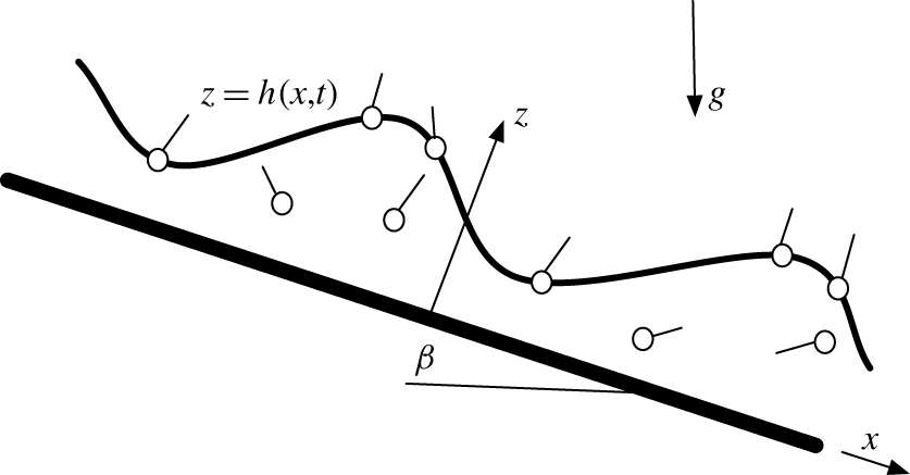
Illustrated in figure 1 is a schematic of the problem under investigation. We are considering the two-dimensional gravity-driven flow of a thin liquid layer doped with a soluble surfactant down a heated incline making an angle  $\unicode[STIX]{x1D6FD}$ with the horizontal. The liquid is taken to be a viscous, incompressible, Newtonian fluid. The incline is maintained at a temperature
 $T_{0}$ while the constant ambient temperature is taken to be
 $T_{a}<T_{0}$. A rectangular coordinate system
 $(x,z)$ has been adopted whereby the position of the free surface of the liquid layer corresponds to
 $z=h(x,t)$.
The flow set-up.

We assume that a fixed mass of surfactant is added to the liquid layer. Since we are dealing with a soluble surfactant, we must consider two separate concentrations: one for the surfactant adsorbed at the surface and another for the surfactant dissolved into the bulk of the layer. Further, we will assume that the surfactant concentrations are below the critical level for the formation of micelles, and thus, the surfactant added to the liquid will exist as monomers. Governing the conservation of surfactant mass in the bulk is the advection–diffusion equation given by
 $$\begin{eqnarray}\frac{\unicode[STIX]{x2202}c}{\unicode[STIX]{x2202}t}+u\frac{\unicode[STIX]{x2202}c}{\unicode[STIX]{x2202}x}+w\frac{\unicode[STIX]{x2202}c}{\unicode[STIX]{x2202}z}=D_{b}\left(\frac{\unicode[STIX]{x2202}^{2}c}{\unicode[STIX]{x2202}x^{2}}+\frac{\unicode[STIX]{x2202}^{2}c}{\unicode[STIX]{x2202}z^{2}}\right),\end{eqnarray}$$
where  $c$ is the concentration of surfactant dissolved in the bulk,
 $D_{b}$ is the molecular diffusivity and
 $(u,w)$ are the velocity components. In order to describe the transport of surfactant adsorbed at the surface we implement the following equation derived by Pereira & Kalliadasis (Reference Pereira and Kalliadasis2011)
 $$\begin{eqnarray}\displaystyle & & \displaystyle \displaystyle {\displaystyle \frac{\unicode[STIX]{x2202}\unicode[STIX]{x1D6E4}}{\unicode[STIX]{x2202}t}}+u{\displaystyle \frac{\unicode[STIX]{x2202}\unicode[STIX]{x1D6E4}}{\unicode[STIX]{x2202}x}}+{\displaystyle \frac{\unicode[STIX]{x1D6E4}}{1+\left({\displaystyle \frac{\unicode[STIX]{x2202}h}{\unicode[STIX]{x2202}x}}\right)^{2}}}\left[{\displaystyle \frac{\unicode[STIX]{x2202}u}{\unicode[STIX]{x2202}x}}+\left({\displaystyle \frac{\unicode[STIX]{x2202}h}{\unicode[STIX]{x2202}x}}\right)\left({\displaystyle \frac{\unicode[STIX]{x2202}w}{\unicode[STIX]{x2202}x}}\right)+{\displaystyle \frac{\unicode[STIX]{x2202}h}{\unicode[STIX]{x2202}x}}\left({\displaystyle \frac{\unicode[STIX]{x2202}u}{\unicode[STIX]{x2202}z}}+{\displaystyle \frac{\unicode[STIX]{x2202}h}{\unicode[STIX]{x2202}x}}{\displaystyle \frac{\unicode[STIX]{x2202}w}{\unicode[STIX]{x2202}z}}\right)\right]\nonumber\\ \displaystyle & & \displaystyle \quad =\displaystyle \frac{D_{s}}{\sqrt{1+\left({\displaystyle \frac{\unicode[STIX]{x2202}h}{\unicode[STIX]{x2202}x}}\right)^{2}}}{\displaystyle \frac{\unicode[STIX]{x2202}}{\unicode[STIX]{x2202}x}}\left({\displaystyle \frac{{\displaystyle \frac{\unicode[STIX]{x2202}\unicode[STIX]{x1D6E4}}{\unicode[STIX]{x2202}x}}}{\sqrt{1+\left({\displaystyle \frac{\unicode[STIX]{x2202}h}{\unicode[STIX]{x2202}x}}\right)^{2}}}}\right)+J_{ba},\nonumber\end{eqnarray}$$
where  $\unicode[STIX]{x1D6E4}(x,t)$ is the surface surfactant concentration,
 $D_{s}$ is the surface molecular diffusivity and
 $J_{ba}$ denotes the net flux of surfactant adsorbed at the surface. If we assume that the rate of adsorption is proportional to the concentration in the bulk, and that the rate of desorption is proportional to the surface concentration, then
 $$\begin{eqnarray}J_{ba}=k_{1}\left(1-\frac{\unicode[STIX]{x1D6E4}}{\unicode[STIX]{x1D6E4}_{\infty }}\right)c-k_{2}\unicode[STIX]{x1D6E4}\quad \text{at }z=h(x,t),\end{eqnarray}$$
where  $k_{1}$ and
 $k_{2}$ are the adsorption and desorption reaction rates, respectively, and
 $\unicode[STIX]{x1D6E4}_{\infty }$ denotes the maximal packing surface concentration. Since the adsorption flux to the surface must also equal the surfactant flux from the bulk and since it is assumed to obey Fickian diffusion,
 $J_{ba}$ can be expressed as
 $$\begin{eqnarray}J_{ba}={\displaystyle \frac{D_{b}}{\sqrt{1+\left({\displaystyle \frac{\unicode[STIX]{x2202}h}{\unicode[STIX]{x2202}x}}\right)^{2}}}}\left({\displaystyle \frac{\unicode[STIX]{x2202}h}{\unicode[STIX]{x2202}x}}{\displaystyle \frac{\unicode[STIX]{x2202}c}{\unicode[STIX]{x2202}x}}-{\displaystyle \frac{\unicode[STIX]{x2202}c}{\unicode[STIX]{x2202}z}}\right)\quad \text{at }z=h(x,t).\end{eqnarray}$$
Regarding the variation in surface tension,  $\unicode[STIX]{x1D70E}$, we will allow it to vary linearly with both the surface surfactant concentration and the surface temperature as follows
 $$\begin{eqnarray}\unicode[STIX]{x1D70E}(\unicode[STIX]{x1D6E4},T)=\unicode[STIX]{x1D70E}_{0}-\unicode[STIX]{x1D70E}_{\unicode[STIX]{x1D6E4}}(\unicode[STIX]{x1D6E4}-\unicode[STIX]{x1D6E4}_{E})-\unicode[STIX]{x1D70E}_{T}(T-T_{a}),\end{eqnarray}$$
where  $\unicode[STIX]{x1D6E4}_{E}$ is the equilibrium surface concentration and
 $\unicode[STIX]{x1D70E}_{0}=\unicode[STIX]{x1D70E}(\unicode[STIX]{x1D6E4}_{E},T_{a})$. The parameters
 $\unicode[STIX]{x1D70E}_{\unicode[STIX]{x1D6E4}}$ and
 $\unicode[STIX]{x1D70E}_{T}$ are evaluated at
 $\unicode[STIX]{x1D6E4}=\unicode[STIX]{x1D6E4}_{E}$,
 $T=T_{a}$ and are defined by
 $$\begin{eqnarray}\unicode[STIX]{x1D70E}_{\unicode[STIX]{x1D6E4}}=-{\displaystyle \frac{\unicode[STIX]{x2202}\unicode[STIX]{x1D70E}}{\unicode[STIX]{x2202}\unicode[STIX]{x1D6E4}}},\quad \unicode[STIX]{x1D70E}_{T}=-{\displaystyle \frac{\unicode[STIX]{x2202}\unicode[STIX]{x1D70E}}{\unicode[STIX]{x2202}T}}.\end{eqnarray}$$
They can be deduced from the equation of state for the surface tension for which there appear to be two commonly used expressions,
 $$\begin{eqnarray}\displaystyle \unicode[STIX]{x1D70E}=\unicode[STIX]{x1D70E}_{p}[1+\unicode[STIX]{x1D6E4}(\unicode[STIX]{x1D6F4}^{1/3}-1)]^{-3} & & \displaystyle \nonumber\end{eqnarray}$$
known as the Sheludko (Reference Sheludko1967) equation, and
 $$\begin{eqnarray}\displaystyle \displaystyle \unicode[STIX]{x1D70E}=\unicode[STIX]{x1D70E}_{p}+RT\unicode[STIX]{x1D6E4}_{\infty }\ln \left(1-\frac{\unicode[STIX]{x1D6E4}}{\unicode[STIX]{x1D6E4}_{\infty }}\right) & & \displaystyle \nonumber\end{eqnarray}$$
known as the von Szyszkowski equation (Nepomnyashchy, Velarde & Colinet Reference Nepomnyashchy, Velarde and Colinet2002).
Here,  $\unicode[STIX]{x1D70E}_{p}$ refers to the surface tension of a surfactant-free, or pure, liquid,
 $R$ is the ideal gas constant,
 $T$ is the temperature in Kelvin and
 $\unicode[STIX]{x1D6F4}$ denotes the ratio of
 $\unicode[STIX]{x1D70E}_{p}$ to the value corresponding to the maximal packing of surfactants. Since our interest is in the variation of surface tension with both surface surfactant concentration and surface temperature we will use the second expression; hence,
 $$\begin{eqnarray}\unicode[STIX]{x1D70E}_{\unicode[STIX]{x1D6E4}}={\displaystyle \frac{RT_{a}\unicode[STIX]{x1D6E4}_{\infty }}{\unicode[STIX]{x1D6E4}_{\infty }-\unicode[STIX]{x1D6E4}_{E}}}\quad \text{and}\quad \unicode[STIX]{x1D70E}_{T}=-R\unicode[STIX]{x1D6E4}_{\infty }\ln \left(1-{\displaystyle \frac{\unicode[STIX]{x1D6E4}_{E}}{\unicode[STIX]{x1D6E4}_{\infty }}}\right).\end{eqnarray}$$
We note that the von Szyszkowski equation becomes singular as  $\unicode[STIX]{x1D6E4}\rightarrow \unicode[STIX]{x1D6E4}_{\infty }^{-}$. Since an underlying assumption is that the surfactant concentration remains below the critical level for the formation of micelles this singularity is of little consequence as
 $\unicode[STIX]{x1D6E4}$ will be well below
 $\unicode[STIX]{x1D6E4}_{\infty }$.
The conservation of mass, momentum and energy equations become (Spurk & Aksel Reference Spurk and Aksel2008)
 $$\begin{eqnarray}\displaystyle & \displaystyle \frac{\unicode[STIX]{x2202}u}{\unicode[STIX]{x2202}x}+\frac{\unicode[STIX]{x2202}w}{\unicode[STIX]{x2202}z}=0, & \displaystyle \nonumber\\ \displaystyle & \displaystyle \unicode[STIX]{x1D70C}\left(\frac{\unicode[STIX]{x2202}u}{\unicode[STIX]{x2202}t}+u\frac{\unicode[STIX]{x2202}u}{\unicode[STIX]{x2202}x}+w\frac{\unicode[STIX]{x2202}u}{\unicode[STIX]{x2202}z}\right)=-\frac{\unicode[STIX]{x2202}p}{\unicode[STIX]{x2202}x}+\unicode[STIX]{x1D70C}g\sin \unicode[STIX]{x1D6FD}+\unicode[STIX]{x1D707}\left(\frac{\unicode[STIX]{x2202}^{2}u}{\unicode[STIX]{x2202}x^{2}}+\frac{\unicode[STIX]{x2202}^{2}u}{\unicode[STIX]{x2202}z^{2}}\right), & \displaystyle \nonumber\\ \displaystyle & \displaystyle \unicode[STIX]{x1D70C}\left(\frac{\unicode[STIX]{x2202}w}{\unicode[STIX]{x2202}t}+u\frac{\unicode[STIX]{x2202}w}{\unicode[STIX]{x2202}x}+w\frac{\unicode[STIX]{x2202}w}{\unicode[STIX]{x2202}z}\right)=-\frac{\unicode[STIX]{x2202}p}{\unicode[STIX]{x2202}z}-\unicode[STIX]{x1D70C}g\cos \unicode[STIX]{x1D6FD}+\unicode[STIX]{x1D707}\left(\frac{\unicode[STIX]{x2202}^{2}w}{\unicode[STIX]{x2202}x^{2}}+\frac{\unicode[STIX]{x2202}^{2}w}{\unicode[STIX]{x2202}z^{2}}\right), & \displaystyle \nonumber\\ \displaystyle & \displaystyle \frac{\unicode[STIX]{x2202}T}{\unicode[STIX]{x2202}t}+u\frac{\unicode[STIX]{x2202}T}{\unicode[STIX]{x2202}x}+w\frac{\unicode[STIX]{x2202}T}{\unicode[STIX]{x2202}z}=\unicode[STIX]{x1D705}\left(\frac{\unicode[STIX]{x2202}^{2}T}{\unicode[STIX]{x2202}x^{2}}+\frac{\unicode[STIX]{x2202}^{2}T}{\unicode[STIX]{x2202}z^{2}}\right), & \displaystyle \nonumber\end{eqnarray}$$
where  $p$ is the pressure,
 $g$ is the acceleration due to gravity,
 $\unicode[STIX]{x1D70C}$ is the density,
 $\unicode[STIX]{x1D707}$ is the dynamic viscosity and
 $\unicode[STIX]{x1D705}$ is the thermal diffusivity.
We next cast the governing equations in dimensionless form. In order to achieve this we choose the Nusselt thickness of a pure liquid given by
 $$\begin{eqnarray}H=\left({\displaystyle \frac{3\unicode[STIX]{x1D707}Q}{g\unicode[STIX]{x1D70C}\sin \unicode[STIX]{x1D6FD}}}\right)^{1/3},\end{eqnarray}$$
as a length scale. In the above  $Q$ denotes the prescribed flow rate. As for the surfactant concentration, there are two possible scales:
 $\unicode[STIX]{x1D6E4}_{\infty }$ and
 $\unicode[STIX]{x1D6E4}_{E}$. We have decided to use the maximal value,
 $\unicode[STIX]{x1D6E4}_{\infty }$. In the study conducted by Pereira & Kalliadasis (Reference Pereira and Kalliadasis2008) they have opted to use
 $\unicode[STIX]{x1D6E4}_{E}$. For the pressure we use
 $\unicode[STIX]{x1D70C}Q^{2}/H^{2}$ as the scale. Using these scales we apply the following transformation
 $$\begin{eqnarray}\begin{array}{@{}c@{}}(x,z)=H(x^{\ast },z^{\ast }),\quad h=Hh^{\ast },\quad t=\displaystyle \frac{H^{2}}{Q}t^{\ast },\quad (u,w)=\displaystyle \frac{Q}{H}(u^{\ast },w^{\ast }),\quad \\ p-p_{a}=\displaystyle \frac{\unicode[STIX]{x1D70C}Q^{2}}{H^{2}}p^{\ast },\quad \unicode[STIX]{x1D6E4}=\unicode[STIX]{x1D6E4}_{\infty }\unicode[STIX]{x1D6E4}^{\ast },\quad c=\displaystyle \frac{\unicode[STIX]{x1D6E4}_{\infty }}{H}c^{\ast },\end{array}\end{eqnarray}$$
where  $p_{a}$ refers to the constant ambient pressure. Lastly, the temperature is scaled according to
 $$\begin{eqnarray}T=T_{a}+(\unicode[STIX]{x0394}T)T^{\ast },\end{eqnarray}$$
where  $\unicode[STIX]{x0394}T=T_{0}-T_{a}$.
With these scalings in place, and dropping the asterisks for notational convenience, the dimensionless equations within the liquid layer become
 $$\begin{eqnarray}\displaystyle & \displaystyle {\displaystyle \frac{\unicode[STIX]{x2202}u}{\unicode[STIX]{x2202}x}}+{\displaystyle \frac{\unicode[STIX]{x2202}w}{\unicode[STIX]{x2202}z}}=0, & \displaystyle\end{eqnarray}$$
 $$\begin{eqnarray}\displaystyle & \displaystyle Re{\displaystyle \frac{\text{D}u}{\text{D}t}}=-Re{\displaystyle \frac{\unicode[STIX]{x2202}p}{\unicode[STIX]{x2202}x}}+{\displaystyle \frac{\unicode[STIX]{x2202}^{2}u}{\unicode[STIX]{x2202}x^{2}}}+{\displaystyle \frac{\unicode[STIX]{x2202}^{2}u}{\unicode[STIX]{x2202}z^{2}}}+3, & \displaystyle\end{eqnarray}$$
 $$\begin{eqnarray}\displaystyle & \displaystyle Re\frac{\text{D}w}{\text{D}t}=-Re{\displaystyle \frac{\unicode[STIX]{x2202}p}{\unicode[STIX]{x2202}z}}+{\displaystyle \frac{\unicode[STIX]{x2202}^{2}w}{\unicode[STIX]{x2202}x^{2}}}+{\displaystyle \frac{\unicode[STIX]{x2202}^{2}w}{\unicode[STIX]{x2202}z^{2}}}-3\cot \unicode[STIX]{x1D6FD}, & \displaystyle\end{eqnarray}$$
 $$\begin{eqnarray}\displaystyle & \displaystyle Pe_{b}\frac{\text{D}c}{\text{D}t}={\displaystyle \frac{\unicode[STIX]{x2202}^{2}c}{\unicode[STIX]{x2202}x^{2}}}+{\displaystyle \frac{\unicode[STIX]{x2202}^{2}c}{\unicode[STIX]{x2202}z^{2}}}, & \displaystyle\end{eqnarray}$$
 $$\begin{eqnarray}\displaystyle & \displaystyle PrRe{\displaystyle \frac{\text{D}T}{\text{D}t}}={\displaystyle \frac{\unicode[STIX]{x2202}^{2}T}{\unicode[STIX]{x2202}x^{2}}}+{\displaystyle \frac{\unicode[STIX]{x2202}^{2}T}{\unicode[STIX]{x2202}z^{2}}}, & \displaystyle\end{eqnarray}$$
where  $Pe_{b}=Q/D_{b}$ is the Péclet number,
 $Pr=\unicode[STIX]{x1D707}/\unicode[STIX]{x1D70C}\unicode[STIX]{x1D705}$ is the Prandtl number,
 $Re=\unicode[STIX]{x1D70C}Q/\unicode[STIX]{x1D707}$ is the Reynolds number and
 $\text{D}/\text{D}t$ denotes the two-dimensional material derivative. Also, along the free surface the dimensionless equation for the surfactant transport takes the form
 $$\begin{eqnarray}\displaystyle & & \displaystyle \displaystyle \frac{\unicode[STIX]{x2202}\unicode[STIX]{x1D6E4}}{\unicode[STIX]{x2202}t}+\frac{\unicode[STIX]{x2202}\unicode[STIX]{x1D6E4}}{\unicode[STIX]{x2202}x}u+\frac{\unicode[STIX]{x1D6E4}}{1+\left({\displaystyle \frac{\unicode[STIX]{x2202}h}{\unicode[STIX]{x2202}x}}\right)^{2}}\left[\frac{\unicode[STIX]{x2202}u}{\unicode[STIX]{x2202}x}+\frac{\unicode[STIX]{x2202}h}{\unicode[STIX]{x2202}x}{\displaystyle \frac{\unicode[STIX]{x2202}w}{\unicode[STIX]{x2202}x}}+\frac{\unicode[STIX]{x2202}h}{\unicode[STIX]{x2202}x}\left({\displaystyle \frac{\unicode[STIX]{x2202}u}{\unicode[STIX]{x2202}z}}+\frac{\unicode[STIX]{x2202}h}{\unicode[STIX]{x2202}x}{\displaystyle \frac{\unicode[STIX]{x2202}w}{\unicode[STIX]{x2202}z}}\right)\right]\nonumber\\ \displaystyle & & \displaystyle \quad =\displaystyle {\displaystyle \frac{1}{Pe_{s}\sqrt{1+\left({\displaystyle \frac{\unicode[STIX]{x2202}h}{\unicode[STIX]{x2202}x}}\right)^{2}}}}{\displaystyle \frac{\unicode[STIX]{x2202}}{\unicode[STIX]{x2202}x}}\left({\displaystyle \frac{{\displaystyle \frac{\unicode[STIX]{x2202}\unicode[STIX]{x1D6E4}}{\unicode[STIX]{x2202}x}}}{\sqrt{1+\left({\displaystyle \frac{\unicode[STIX]{x2202}h}{\unicode[STIX]{x2202}x}}\right)^{2}}}}\right)+k_{s}[\unicode[STIX]{x1D709}_{s}(1-\unicode[STIX]{x1D6E4})c-\unicode[STIX]{x1D6E4}]\quad \text{at }z=h(x,t),\nonumber\\ \displaystyle & & \displaystyle\end{eqnarray}$$
where  $Pe_{s}=Q/D_{s}$,
 $k_{s}=Hk_{2}/U$ and
 $\unicode[STIX]{x1D709}_{s}=k_{1}/k_{2}H$.
The system of equations (2.1)–(2.5) is to be solved subject to the following boundary conditions. Along the free surface  $z=h(x,t)$ we impose the dynamic conditions
 $$\begin{eqnarray}\displaystyle p & = & \displaystyle \displaystyle {\displaystyle \frac{2}{Re\left(1+\left({\displaystyle \frac{\unicode[STIX]{x2202}h}{\unicode[STIX]{x2202}x}}\right)^{2}\right)}}\left[{\displaystyle \frac{\unicode[STIX]{x2202}u}{\unicode[STIX]{x2202}x}}\left(\left({\displaystyle \frac{\unicode[STIX]{x2202}h}{\unicode[STIX]{x2202}x}}\right)^{2}-1\right)-{\displaystyle \frac{\unicode[STIX]{x2202}h}{\unicode[STIX]{x2202}x}}\left({\displaystyle \frac{\unicode[STIX]{x2202}u}{\unicode[STIX]{x2202}z}}+{\displaystyle \frac{\unicode[STIX]{x2202}w}{\unicode[STIX]{x2202}x}}\right)\right]\nonumber\\ \displaystyle & & \displaystyle -\,\displaystyle {\displaystyle \frac{{\displaystyle \frac{\unicode[STIX]{x2202}^{2}h}{\unicode[STIX]{x2202}x^{2}}}}{\left(1+\left({\displaystyle \frac{\unicode[STIX]{x2202}h}{\unicode[STIX]{x2202}x}}\right)^{2}\right)^{3/2}}}\left[We-M_{1}\left(\unicode[STIX]{x1D6E4}-\unicode[STIX]{x1D6E4}_{E}\right)-M_{2}T\right],\end{eqnarray}$$
 $$\begin{eqnarray}\displaystyle & & \displaystyle \displaystyle -\,Re\sqrt{1+\left({\displaystyle \frac{\unicode[STIX]{x2202}h}{\unicode[STIX]{x2202}x}}\right)^{2}}\left[M_{1}\frac{\unicode[STIX]{x2202}\unicode[STIX]{x1D6E4}}{\unicode[STIX]{x2202}x}+M_{2}\left(\frac{\unicode[STIX]{x2202}T}{\unicode[STIX]{x2202}x}+\frac{\unicode[STIX]{x2202}h}{\unicode[STIX]{x2202}x}\frac{\unicode[STIX]{x2202}T}{\unicode[STIX]{x2202}z}\right)\right]\nonumber\\ \displaystyle & & \displaystyle \qquad =\displaystyle \left(1-\left(\frac{\unicode[STIX]{x2202}h}{\unicode[STIX]{x2202}x}\right)^{2}\right)\left(\frac{\unicode[STIX]{x2202}w}{\unicode[STIX]{x2202}x}+\frac{\unicode[STIX]{x2202}u}{\unicode[STIX]{x2202}z}\right)-4\frac{\unicode[STIX]{x2202}h}{\unicode[STIX]{x2202}x}\frac{\unicode[STIX]{x2202}u}{\unicode[STIX]{x2202}x},\end{eqnarray}$$
 $$\begin{eqnarray}\displaystyle \displaystyle \frac{1}{Pe_{b}\sqrt{1+\left({\displaystyle \frac{\unicode[STIX]{x2202}h}{\unicode[STIX]{x2202}x}}\right)^{2}}}\left({\displaystyle \frac{\unicode[STIX]{x2202}h}{\unicode[STIX]{x2202}x}}{\displaystyle \frac{\unicode[STIX]{x2202}c}{\unicode[STIX]{x2202}x}}-{\displaystyle \frac{\unicode[STIX]{x2202}c}{\unicode[STIX]{x2202}z}}\right)=k_{s}[\unicode[STIX]{x1D709}_{s}(1-\unicode[STIX]{x1D6E4})c-\unicode[STIX]{x1D6E4}], & & \displaystyle\end{eqnarray}$$
and
 $$\begin{eqnarray}-BT\sqrt{1+\left(\frac{\unicode[STIX]{x2202}h}{\unicode[STIX]{x2202}x}\right)^{2}}=\frac{\unicode[STIX]{x2202}T}{\unicode[STIX]{x2202}z}-\frac{\unicode[STIX]{x2202}h}{\unicode[STIX]{x2202}x}\frac{\unicode[STIX]{x2202}T}{\unicode[STIX]{x2202}x}.\end{eqnarray}$$
Conditions (2.7) and (2.8) arise from a balance between the ambient pressure and surface tension, condition (2.9) refers to balance between the surfactant adsorption flux and the diffusive flux from the bulk, while condition (2.10) is essentially a statement of Newton’s law of cooling. Here,  $We=\unicode[STIX]{x1D70E}_{0}H/\unicode[STIX]{x1D70C}Q^{2}$,
 $M_{1}=\unicode[STIX]{x1D70E}_{\unicode[STIX]{x1D6E4}}H\unicode[STIX]{x1D6E4}_{\infty }/\unicode[STIX]{x1D70C}Q^{2}$,
 $M_{2}=\unicode[STIX]{x1D70E}_{T}H\unicode[STIX]{x0394}T/\unicode[STIX]{x1D70C}Q^{2}$ and
 $B=\unicode[STIX]{x1D6FC}_{g}H/\unicode[STIX]{x1D70C}c_{p}\unicode[STIX]{x1D705}$ with
 $\unicode[STIX]{x1D6FC}_{g}$ denoting the heat transfer coefficient across the liquid–air interface and
 $c_{p}$ is the specific heat at constant pressure of the liquid. Ignoring evaporation the kinematic condition along the free surface is given by
 $$\begin{eqnarray}w=\frac{\unicode[STIX]{x2202}h}{\unicode[STIX]{x2202}t}+u\frac{\unicode[STIX]{x2202}h}{\unicode[STIX]{x2202}x},\quad \text{at }z=h(x,t).\end{eqnarray}$$
Lastly, along the incline  $z=0$ we apply the no-slip, impermeability and constant temperature conditions
 $$\begin{eqnarray}u=w=\frac{\unicode[STIX]{x2202}c}{\unicode[STIX]{x2202}z}=0\quad \text{and}\quad T=1.\end{eqnarray}$$
3 Linear stability analysis
In this section we will investigate the stability of a unidirectional steady flow which is constant in the streamwise direction. Setting all derivatives with respect to  $x$ and
 $t$ to zero one easily obtains
 $$\begin{eqnarray}\displaystyle & \displaystyle \unicode[STIX]{x1D6E4}=\unicode[STIX]{x1D6E4}_{E}=\text{const.},\quad c=c_{E}\equiv \frac{\unicode[STIX]{x1D6E4}_{E}}{\unicode[STIX]{x1D709}_{s}(1-\unicode[STIX]{x1D6E4}_{E})},\quad h=1,\quad w=0, & \displaystyle \nonumber\\ \displaystyle & \displaystyle u=u_{E}(z)\equiv 3\left(z-{\displaystyle \frac{z^{2}}{2}}\right),\quad p=p_{E}(z)\equiv -{\displaystyle \frac{3\cot \unicode[STIX]{x1D6FD}}{Re}}(z-1),\quad T=T_{E}(z)\equiv 1-{\displaystyle \frac{Bz}{(1+B)}}, & \displaystyle \nonumber\end{eqnarray}$$
where  $\unicode[STIX]{x1D6E4}_{E}$ assumes the role of a control parameter in the range
 $0\leqslant \unicode[STIX]{x1D6E4}_{E}\leqslant 1$. Clearly, in order for
 $c_{E}$ to remain bounded as
 $\unicode[STIX]{x1D6E4}_{E}\rightarrow 1^{-}$ it follows that we must also have
 $\unicode[STIX]{x1D709}_{s}\rightarrow \infty$ (i.e. an insoluble surfactant) such that the product
 $\unicode[STIX]{x1D709}_{s}(1-\unicode[STIX]{x1D6E4}_{E})$ does not approach zero. More specifically, since we expect the surfactant concentration in the bulk to vanish in the insoluble limit, the product
 $\unicode[STIX]{x1D709}_{s}(1-\unicode[STIX]{x1D6E4}_{E})$ must approach infinity. This suggests that a maximal surface concentration can only be attained if the surfactant is insoluble. Following Pascal et al. (Reference Pascal, D’Alessio and Ellaban2019) we will use
 $M_{tot}=\unicode[STIX]{x1D6E4}_{E}+c_{E}$ as a control parameter instead of
 $\unicode[STIX]{x1D6E4}_{E}$ which are related by the following expression
 $$\begin{eqnarray}\unicode[STIX]{x1D6E4}_{E}=\frac{1}{2}\left(1+M_{tot}+\frac{1}{\unicode[STIX]{x1D709}_{s}}-\sqrt{(M_{tot}-1)^{2}+\frac{2}{\unicode[STIX]{x1D709}_{s}}(M_{tot}+1)+\frac{1}{\unicode[STIX]{x1D709}_{s}^{2}}}\right).\end{eqnarray}$$
The control parameters then become  $M_{tot}$,
 $\unicode[STIX]{x1D709}_{s}$,
 $k_{s}$,
 $\unicode[STIX]{x1D6FD}$,
 $Pe_{b}$,
 $Pe_{s}$,
 $Pr$,
 $B$,
 $M_{1}$,
 $M_{2}$,
 $We$ and
 $Re$.
To conduct a linear stability analysis we begin by disturbing the steady solution by adding an infinitesimal perturbation as follows
 $$\begin{eqnarray}\begin{array}{@{}c@{}}u=u_{E}+\tilde{u} ,\quad w=\tilde{w},\quad p=p_{E}+\tilde{p},\quad h=1+\tilde{h},\quad \\ \unicode[STIX]{x1D6E4}=\unicode[STIX]{x1D6E4}_{E}+\tilde{\unicode[STIX]{x1D6E4}},\quad c=c_{E}+\tilde{c},\quad T=T_{E}+\tilde{T},\end{array}\end{eqnarray}$$
where the tildes denote the perturbations. Next, we substitute these expressions into the governing equations and linearize with respect to the perturbations. To simplify the analysis we introduce the streamfunction,  $\unicode[STIX]{x1D713}$, such that
 $$\begin{eqnarray}\tilde{u} =\frac{\unicode[STIX]{x2202}\unicode[STIX]{x1D713}}{\unicode[STIX]{x2202}z},\quad \tilde{w}=-\frac{\unicode[STIX]{x2202}\unicode[STIX]{x1D713}}{\unicode[STIX]{x2202}x}.\end{eqnarray}$$
This guarantees that the continuity equation is automatically satisfied. We then eliminate the pressure perturbation by combining the momentum equations and employ normal modes given by
 $$\begin{eqnarray}(\unicode[STIX]{x1D713},\tilde{c},\tilde{\unicode[STIX]{x1D6E4}},\tilde{T},\tilde{h})=(\unicode[STIX]{x1D6F9}(z),{\hat{c}}(z),\hat{\unicode[STIX]{x1D6E4}},\hat{T}(z),\unicode[STIX]{x1D702})\text{e}^{\text{i}k(x-vt)},\end{eqnarray}$$
where the perturbation wavenumber,  $k$, is taken to be real and positive, while
 $v$ is a complex quantity with the real part denoting the phase speed and the imaginary part, Im(
 $v$), is related to the growth rate.
The functions  $\unicode[STIX]{x1D6F9}(z)$,
 ${\hat{c}}(z)$ and
 $\hat{T}(z)$ satisfy the following Orr–Sommerfeld type ordinary differential equations over the domain
 $0<z<1$
 $$\begin{eqnarray}\displaystyle & \displaystyle D^{4}\unicode[STIX]{x1D6F9}-[\text{i}kRe(u_{E}-v)+k^{2}]D^{2}\unicode[STIX]{x1D6F9}+[-\text{i}k^{3}Re(u_{E}-v)+k^{4}+\text{i}kReD^{2}u_{E}]\unicode[STIX]{x1D6F9}=0, & \displaystyle\end{eqnarray}$$
 $$\begin{eqnarray}\displaystyle & \displaystyle \text{i}kPe_{b}(u_{E}-v){\hat{c}}=D^{2}{\hat{c}}-k^{2}{\hat{c}}, & \displaystyle\end{eqnarray}$$
 $$\begin{eqnarray}\displaystyle & \displaystyle \text{i}kPrRe(u_{E}-v)\hat{T}=D^{2}\hat{T}-k^{2}\hat{T}+\text{i}kPe(DT_{E})\unicode[STIX]{x1D6F9}, & \displaystyle\end{eqnarray}$$
where  $D\equiv \text{d}/\text{d}z$. The associated boundary conditions at
 $z=1$ are
 $$\begin{eqnarray}\displaystyle & \displaystyle D^{3}\unicode[STIX]{x1D6F9}-\left[\text{i}kRe(u_{E}-v)+2k^{2}\right]D\unicode[STIX]{x1D6F9}-\left[3\text{i}k\cot \unicode[STIX]{x1D6FD}+\text{i}k^{3}(We-M_{2}T_{E})\right]\unicode[STIX]{x1D702}=0, & \displaystyle\end{eqnarray}$$
 $$\begin{eqnarray}\displaystyle & \displaystyle -\text{i}kRe(M_{1}\hat{\unicode[STIX]{x1D6E4}}+M_{2}\hat{T})=D^{2}\unicode[STIX]{x1D6F9}+k^{2}\unicode[STIX]{x1D6F9}-(3-\text{i}kReM_{2}DT_{E})\unicode[STIX]{x1D702}, & \displaystyle\end{eqnarray}$$
 $$\begin{eqnarray}\displaystyle & \displaystyle \text{i}k(u_{E}-v)\hat{\unicode[STIX]{x1D6E4}}+\text{i}k\unicode[STIX]{x1D6E4}_{E}D\unicode[STIX]{x1D6F9}=-{\displaystyle \frac{k^{2}}{Pe_{s}}}\hat{\unicode[STIX]{x1D6E4}}+k_{s}[\unicode[STIX]{x1D709}_{s}(1-\unicode[STIX]{x1D6E4}_{E}){\hat{c}}-(1+\unicode[STIX]{x1D709}_{s}c_{E})\hat{\unicode[STIX]{x1D6E4}}], & \displaystyle\end{eqnarray}$$
 $$\begin{eqnarray}\displaystyle & \displaystyle -D{\hat{c}}=Pe_{b}k_{s}[\unicode[STIX]{x1D709}_{s}(1-\unicode[STIX]{x1D6E4}_{E}){\hat{c}}-(1+\unicode[STIX]{x1D709}_{s}c_{E})\hat{\unicode[STIX]{x1D6E4}}], & \displaystyle\end{eqnarray}$$
 $$\begin{eqnarray}\displaystyle & \displaystyle D\hat{T}+B\hat{T}=-BDT_{E}\unicode[STIX]{x1D702}, & \displaystyle\end{eqnarray}$$
and
 $$\begin{eqnarray}-\unicode[STIX]{x1D6F9}=(u_{E}-v)\unicode[STIX]{x1D702}.\end{eqnarray}$$
At  $z=0$ we have
 $$\begin{eqnarray}\unicode[STIX]{x1D6F9}=D\unicode[STIX]{x1D6F9}=D{\hat{c}}=\hat{T}=0.\end{eqnarray}$$
The problem posed by (3.2)–(3.11) represents an eigenvalue problem with  $v$ denoting the eigenvalue which signals if the disturbance with wavenumber
 $k$ will be amplified or damped in time for a given set of flow parameters. The system of (3.2)–(3.11) will be solved asymptotically as
 $k\rightarrow 0$ (i.e. longwave perturbations) and also numerically with no restriction on
 $k$.
3.1 Asymptotic solution
In carrying out the asymptotic analysis we begin by expanding the flow variables in powers of  $k$ as follows
 $$\begin{eqnarray}\displaystyle & \displaystyle \unicode[STIX]{x1D6F9}=\unicode[STIX]{x1D6F9}_{0}(z)+k\unicode[STIX]{x1D6F9}_{1}(z)+\cdots \,, & \displaystyle \nonumber\\ \displaystyle & \displaystyle {\hat{c}}=c_{0}(z)+kc_{1}(z)+\cdots \,, & \displaystyle \nonumber\\ \displaystyle & \displaystyle \hat{T}=T_{0}(z)+kT_{1}(z)+\cdots \,, & \displaystyle \nonumber\\ \displaystyle & \displaystyle \hat{\unicode[STIX]{x1D6E4}}=\unicode[STIX]{x1D6E4}_{0}+k\unicode[STIX]{x1D6E4}_{1}+\cdots \,, & \displaystyle \nonumber\\ \displaystyle & \displaystyle \unicode[STIX]{x1D702}=\unicode[STIX]{x1D702}_{0}+k\unicode[STIX]{x1D702}_{1}+\cdots \,, & \displaystyle \nonumber\\ \displaystyle & \displaystyle v=v_{0}+kv_{1}+\cdots & \displaystyle \nonumber\end{eqnarray}$$
Without loss of generality we can normalize the eigenvalue problem and set  $\unicode[STIX]{x1D702}_{0}=1$ and
 $\unicode[STIX]{x1D702}_{1}=\unicode[STIX]{x1D702}_{2}=0$. An immediate consequence is that the perturbed free surface is given by
 $\tilde{h}=\text{e}^{\text{i}k(x-vt)}$. Substituting these expansions into the system (3.2)–(3.11), and assuming that all the parameters to be
 $O(1)$ as
 $k\rightarrow 0$, leads to a hierarchy of problems at various orders of
 $k$ which can be solved sequentially.
The leading-order problem satisfies
 $$\begin{eqnarray}D^{4}\unicode[STIX]{x1D6F9}_{0}=0,\quad D^{2}c_{0}=0,\quad D^{2}T_{0}=0,\end{eqnarray}$$
subject to the boundary conditions
 $$\begin{eqnarray}\displaystyle & \displaystyle D^{3}\unicode[STIX]{x1D6F9}_{0}=0,\quad D^{2}\unicode[STIX]{x1D6F9}_{0}=3,\quad v_{0}=\unicode[STIX]{x1D6F9}_{0}-u_{E},\quad Dc_{0}=0,\quad DT_{0}+BT_{0}=-BDT_{E}\quad \text{at }z=1, & \displaystyle \nonumber\\ \displaystyle & \displaystyle \unicode[STIX]{x1D709}_{s}(1-\unicode[STIX]{x1D6E4}_{E})\unicode[STIX]{x1D719}_{0}=(1+\unicode[STIX]{x1D709}_{s}\unicode[STIX]{x1D719}_{E})\unicode[STIX]{x1D6E4}_{0}\quad \text{at }z=1, & \displaystyle \nonumber\\ \displaystyle & \displaystyle Dc_{0}=\unicode[STIX]{x1D6F9}_{0}=D\unicode[STIX]{x1D6F9}_{0}=0\quad \text{at }z=0. & \displaystyle \nonumber\end{eqnarray}$$
The solutions are easily found to be
 $$\begin{eqnarray}\unicode[STIX]{x1D6F9}_{0}(z)=\frac{3}{2}z^{2},\quad T_{0}(z)=\frac{B^{2}}{(1+B)^{2}}z,\quad \unicode[STIX]{x1D6E4}_{0}=\frac{\unicode[STIX]{x1D709}_{s}(1-\unicode[STIX]{x1D6E4}_{E})}{(1+\unicode[STIX]{x1D709}_{s}c_{E})}c_{0},\quad v_{0}=3,\end{eqnarray}$$
where  $c_{0}$ is a constant which is yet to be determined.
Proceeding to the  $O(k)$ problem yields the system of equations
 $$\begin{eqnarray}\displaystyle & \displaystyle D^{4}\unicode[STIX]{x1D6F9}_{1}=\text{i}Re(u_{E}-v_{0})D^{2}\unicode[STIX]{x1D6F9}_{0}-\text{i}ReD^{2}u_{E}\unicode[STIX]{x1D6F9}_{0}, & \displaystyle \nonumber\\ \displaystyle & \displaystyle D^{2}c_{1}=\text{i}Pe_{b}(u_{E}-v_{0})c_{0}, & \displaystyle \nonumber\\ \displaystyle & \displaystyle D^{2}T_{1}=\text{i}PrRe[(u_{E}-v_{0})T_{0}-DT_{0}\unicode[STIX]{x1D6F9}_{0}], & \displaystyle \nonumber\end{eqnarray}$$
subject to
 $$\begin{eqnarray}\displaystyle & \displaystyle D^{3}\unicode[STIX]{x1D6F9}_{1}=\text{i}Re(u_{E}-v_{0})D\unicode[STIX]{x1D6F9}_{0}+3\text{i}\cot \unicode[STIX]{x1D6FD}\quad \text{at }z=1, & \displaystyle \nonumber\\ \displaystyle & \displaystyle D^{2}\unicode[STIX]{x1D6F9}_{1}=-\text{i}Re(M_{1}\unicode[STIX]{x1D6E4}_{0}+M_{2}T_{0})-\text{i}ReM_{2}DT_{E}\quad \text{at }z=1, & \displaystyle \nonumber\\ \displaystyle & \displaystyle \text{D}c_{1}=-\text{i}Pe_{b}[(u_{E}-v_{0})\unicode[STIX]{x1D6E4}_{0}+\unicode[STIX]{x1D6E4}_{E}D\unicode[STIX]{x1D6F9}_{0}]\quad \text{at }z=1, & \displaystyle \nonumber\\ \displaystyle & \displaystyle \text{D}c_{1}=-k_{s}Pe_{b}[\unicode[STIX]{x1D709}_{s}(1-\unicode[STIX]{x1D6E4}_{E})c_{1}-(1+\unicode[STIX]{x1D709}_{s}c_{E})\unicode[STIX]{x1D6E4}_{1}]\quad \text{at }z=1, & \displaystyle \nonumber\\ \displaystyle & \displaystyle \text{D}T_{1}+BT_{1}=0\quad \text{at }z=1, & \displaystyle \nonumber\\ \displaystyle & \displaystyle \unicode[STIX]{x1D6F9}_{1}=v_{1}\quad \text{at }z=1, & \displaystyle \nonumber\\ \displaystyle & \displaystyle \unicode[STIX]{x1D6F9}_{1}=D\unicode[STIX]{x1D6F9}_{1}(0)=Dc_{1}=T_{1}=0\quad \text{at }z=0. & \displaystyle \nonumber\end{eqnarray}$$
The condition for neutral stability can be obtained from  $v_{1}$ given above in terms of
 $\unicode[STIX]{x1D6F9}_{1}$. The solution for
 $\unicode[STIX]{x1D6F9}_{1}$ was found to be
 $$\begin{eqnarray}\unicode[STIX]{x1D6F9}_{1}(z)=\frac{3\text{i}Re}{40}(z^{5}-5z^{4})+\frac{\text{i}\cot \unicode[STIX]{x1D6FD}}{2}z^{3}+\frac{\text{i}Re}{2}\left[3\left(1-\frac{\cot \unicode[STIX]{x1D6FD}}{Re}\right)-M_{1}\unicode[STIX]{x1D6E4}_{0}+\frac{M_{2}B}{(1+B)^{2}}\right]z^{2},\end{eqnarray}$$
where
 $$\begin{eqnarray}\unicode[STIX]{x1D6E4}_{0}=\frac{6\unicode[STIX]{x1D6E4}_{E}\unicode[STIX]{x1D709}_{s}(1-\unicode[STIX]{x1D6E4}_{E})^{2}}{4+3\unicode[STIX]{x1D709}_{s}(1-\unicode[STIX]{x1D6E4}_{E})^{2}}.\end{eqnarray}$$
Hence,
 $$\begin{eqnarray}v_{1}=\unicode[STIX]{x1D6F9}_{1}(1)=\text{i}Re\left(\frac{6}{5}-\frac{\cot \unicode[STIX]{x1D6FD}}{Re}+\frac{M_{2}B}{2(1+B)^{2}}-\frac{3M_{1}\unicode[STIX]{x1D6E4}_{E}\unicode[STIX]{x1D709}_{s}(1-\unicode[STIX]{x1D6E4}_{E})^{2}}{4+3\unicode[STIX]{x1D709}_{s}(1-\unicode[STIX]{x1D6E4}_{E})^{2}}\right),\end{eqnarray}$$
with the state of neutral stability given by  $v_{1}=0$. It is immediately evident that this relation is independent of the parameters
 $Pr$,
 $Pe_{s}$,
 $Pe_{b}$,
 $We$ and
 $k_{s}$. Therefore the indication is that neutral stability is not affected by solutal and thermal diffusivity, nor is it influenced by the individual desorption and adsorption reaction rates, but only by the ratio of the two, which is given by the parameter
 $\unicode[STIX]{x1D709}_{s}$.
Now, the neutral stability relation can be written as the following expression for the critical Reynolds number,  $Re_{crit}$,
 $$\begin{eqnarray}\frac{\cot \unicode[STIX]{x1D6FD}}{Re_{crit}}-\frac{6}{5}=F(B,\unicode[STIX]{x1D6E4}_{E};M_{1},M_{2},\unicode[STIX]{x1D709}_{s}),\end{eqnarray}$$
where
 $$\begin{eqnarray}F(B,\unicode[STIX]{x1D6E4}_{E};M_{1},M_{2},\unicode[STIX]{x1D709}_{s})=\frac{M_{2}B}{2(1+B)^{2}}-\frac{3M_{1}\unicode[STIX]{x1D6E4}_{E}\unicode[STIX]{x1D709}_{s}(1-\unicode[STIX]{x1D6E4}_{E})^{2}}{4+3\unicode[STIX]{x1D709}_{s}(1-\unicode[STIX]{x1D6E4}_{E})^{2}}.\end{eqnarray}$$
For an isothermal clean liquid layer  $F=0$. The function
 $F$ accounts for departures from
 $F=0$, and hence variations in
 $Re_{crit}$, as a result of heating and doping, and is made up of two terms which clearly identify the contributions made by the thermal Marangoni effect and the soluto Marangoni effect, respectively. It is also clear that heating destabilizes the flow while the addition of a surfactant stabilizes the flow, as expected. We note that
 $F=0$ can also occur when the thermosolutal mechanisms exactly cancel each other which happens when
 $$\begin{eqnarray}\frac{M_{2}B}{2(1+B)^{2}}=\frac{3M_{1}\unicode[STIX]{x1D6E4}_{E}\unicode[STIX]{x1D709}_{s}(1-\unicode[STIX]{x1D6E4}_{E})^{2}}{4+3\unicode[STIX]{x1D709}_{s}(1-\unicode[STIX]{x1D6E4}_{E})^{2}}\quad \text{or}\quad \frac{M_{2}}{M_{1}}=\frac{6\unicode[STIX]{x1D6E4}_{E}\unicode[STIX]{x1D709}_{s}(1+B)^{2}(1-\unicode[STIX]{x1D6E4}_{E})^{2}}{B[4+3\unicode[STIX]{x1D709}_{s}(1-\unicode[STIX]{x1D6E4}_{E})^{2}]}.\end{eqnarray}$$
Thus, linear theory predicts the necessary relationship needed between the parameters in order for a heated liquid layer doped with a surfactant to have the same critical Reynolds number as the corresponding isothermal clean liquid layer.
To determine the extreme values of  $Re_{crit}$ over the semi-infinite rectangular strip
 $0\leqslant B<\infty$,
 $0\leqslant \unicode[STIX]{x1D6E4}_{E}\leqslant 1$ in the
 $B\unicode[STIX]{x1D6E4}_{E}$-plane we first find the critical points of
 $F$ by solving
 $$\begin{eqnarray}\frac{\unicode[STIX]{x2202}F}{\unicode[STIX]{x2202}B}=\frac{\unicode[STIX]{x2202}F}{\unicode[STIX]{x2202}\unicode[STIX]{x1D6E4}_{E}}=0.\end{eqnarray}$$
The critical points are found to be  $(B,\unicode[STIX]{x1D6E4}_{E})=(1,1)$ or
 $(1,\overline{\unicode[STIX]{x1D6E4}}_{E})$ where
 $\overline{\unicode[STIX]{x1D6E4}}_{E}$ is the real root of the cubic equation
 $$\begin{eqnarray}3\unicode[STIX]{x1D709}_{s}\overline{\unicode[STIX]{x1D6E4}}_{E}^{3}-9\unicode[STIX]{x1D709}_{s}\overline{\unicode[STIX]{x1D6E4}}_{E}^{2}+9\unicode[STIX]{x1D709}_{s}\overline{\unicode[STIX]{x1D6E4}}_{E}+12\overline{\unicode[STIX]{x1D6E4}}_{E}-3\unicode[STIX]{x1D709}_{s}-4=0,\end{eqnarray}$$
given by
 $$\begin{eqnarray}\overline{\unicode[STIX]{x1D6E4}}_{E}=1+\frac{a}{3\unicode[STIX]{x1D709}_{s}}-\frac{4}{a}\quad \text{where }a=\left(12\sqrt{3\unicode[STIX]{x1D709}_{s}^{3}(3\unicode[STIX]{x1D709}_{s}+4)}-36\unicode[STIX]{x1D709}_{s}^{2}\right)^{1/3}.\end{eqnarray}$$
It is worth noting that in the insoluble limit as  $\unicode[STIX]{x1D709}_{s}\rightarrow \infty$,
 $\overline{\unicode[STIX]{x1D6E4}}_{E}\rightarrow 1^{-}$ and the two critical points merge. It turns out that the interior critical point
 $(B,\unicode[STIX]{x1D6E4}_{E})=(1,\overline{\unicode[STIX]{x1D6E4}}_{E})$ is a saddle point. Inspecting the values of
 $F$ along the boundary we find that along
 $B=0$ and
 $B\rightarrow \infty$ a minimum value of
 $F$ is assumed given by
 $$\begin{eqnarray}F_{min}=-\frac{3M_{1}\unicode[STIX]{x1D709}_{s}\overline{\unicode[STIX]{x1D6E4}}_{E}(1-\overline{\unicode[STIX]{x1D6E4}}_{E})^{2}}{[4+3\unicode[STIX]{x1D709}_{s}(1-\overline{\unicode[STIX]{x1D6E4}}_{E})^{2}]},\end{eqnarray}$$
while along  $\unicode[STIX]{x1D6E4}_{E}=0$ and
 $\unicode[STIX]{x1D6E4}_{E}=1$ a maximum value of
 $F$ is assumed given by
 $$\begin{eqnarray}F_{max}=\frac{M_{2}}{8}.\end{eqnarray}$$
From this information the extreme values of  $Re_{crit}$ are
 $$\begin{eqnarray}(Re_{crit})_{max}=\frac{5[4+3\unicode[STIX]{x1D709}_{s}(1-\overline{\unicode[STIX]{x1D6E4}}_{E})^{2}]\cot \unicode[STIX]{x1D6FD}}{3[8+\unicode[STIX]{x1D709}_{s}(6-5\overline{\unicode[STIX]{x1D6E4}}_{E}M_{1})(1-\overline{\unicode[STIX]{x1D6E4}}_{E})^{2}]}\quad \text{and}\quad (Re_{crit})_{min}=\frac{40\cot \unicode[STIX]{x1D6FD}}{48+5M_{2}}.\end{eqnarray}$$
The existence of the saddle point  $(B,\unicode[STIX]{x1D6E4}_{E})=(1,\overline{\unicode[STIX]{x1D6E4}}_{E})$ can be explained as follows. If we hold
 $B$ constant at
 $B=1$ and vary
 $\unicode[STIX]{x1D6E4}_{E}$ we note that when
 $\unicode[STIX]{x1D6E4}_{E}=0$ or
 $\unicode[STIX]{x1D6E4}_{E}=1$ we obtain the above minimum value for
 $Re_{crit}$. Now, as we add a surfactant to an initially surfactant-free liquid layer gradients in the concentration will form along the free surface whereby the concentration is higher at the crests than at the troughs. This creates Marangoni stresses (i.e. solutocapillary forces) in the direction of the troughs which are responsible for damping surface deflections, and hence, stabilizing the flow. So a liquid layer with a non-uniform concentration of surface surfactant is more stable (i.e. has a larger
 $Re_{crit}$ value) than a corresponding clean liquid layer because surfactants have a tendency of enhancing the elasticity of the surface. As more surfactant is added to the liquid layer the surface will eventually reach its maximal value. At this point the concentration gradients cannot form along the surface and consequently the liquid layer behaves exactly as a clean heated liquid layer. This is why
 $\unicode[STIX]{x1D6E4}_{E}=0$ and
 $\unicode[STIX]{x1D6E4}_{E}=1$ yield the same
 $Re_{crit}$ value. Thus, there exists an optimal value of
 $\unicode[STIX]{x1D6E4}_{E}$,
 $\unicode[STIX]{x1D6E4}_{E}=\overline{\unicode[STIX]{x1D6E4}}_{E}$, that maximizes
 $Re_{crit}$. Similarly, if we fix the value of
 $\unicode[STIX]{x1D6E4}_{E}=\overline{\unicode[STIX]{x1D6E4}}_{E}$ and vary
 $B$ we observe that when
 $B=0$ or
 $B\rightarrow \infty$ we obtain the above maximum value for
 $Re_{crit}$. The case
 $B=0$ corresponds to an insulated fluid layer which means that the temperature will be uniform throughout the layer. On the other hand, the case
 $B\rightarrow \infty$ corresponds to an infinite rate of heat transfer across the interface which means that the interface temperature will remain fixed at the ambient value. In both of these cases there is no temperature gradient along the free surface, and hence, no Marangoni stresses. Thus, the liquid layer will behave like an isothermal, surfactant-laden liquid layer. Now, as
 $B$ increases from zero a temperature distribution in the liquid layer begins to develop and if the free surface is non-planar, then the temperature along the free surface will be greater at the troughs than at the crests. This temperature gradient creates Marangoni stresses (i.e. thermocapillary forces) which act to amplify the waves on the surface, and hence, destabilize the flow. However, for large
 $B$ the temperature along the free surface will approach that of the ambient medium which is constant, and as such these thermocapillary forces will be weakened. Consequently, there exists a optimal value of
 $B$,
 $B=1$, for which thermocapillarity is maximized resulting in a minimum value for
 $Re_{crit}$.
Alternatively, equation (3.12) can be written as
 $$\begin{eqnarray}Re_{crit}=\frac{10(1+B)^{2}[4+3\unicode[STIX]{x1D709}_{s}(1-\unicode[STIX]{x1D6E4}_{E})^{2}]\cot \unicode[STIX]{x1D6FD}}{6(1+B)^{2}[8+\unicode[STIX]{x1D709}_{s}(6-5\unicode[STIX]{x1D6E4}_{E}M_{1})(1-\unicode[STIX]{x1D6E4}_{E})^{2}]+5M_{2}B[4+3\unicode[STIX]{x1D709}_{s}(1-\unicode[STIX]{x1D6E4}_{E})^{2}]},\end{eqnarray}$$
which can be expressed in terms of  $M_{tot}$ by making use of (3.1). There are various limits that can be taken and comparisons that can be drawn. For example, the isothermal limit can be obtained by setting
 $M_{2}=0$ or
 $B=0$; this yields
 $$\begin{eqnarray}\left.Re_{crit}\right|_{B=0}=\frac{5[4+3\unicode[STIX]{x1D709}_{s}(1-\unicode[STIX]{x1D6E4}_{E})^{2}]\cot \unicode[STIX]{x1D6FD}}{3[8+\unicode[STIX]{x1D709}_{s}(6-5\unicode[STIX]{x1D6E4}_{E}M_{1})(1-\unicode[STIX]{x1D6E4}_{E})^{2}]},\end{eqnarray}$$
which coincides with the result obtained by Pascal et al. (Reference Pascal, D’Alessio and Ellaban2019) and also with Karapetsas & Bontozoglou (Reference Karapetsas and Bontozoglou2014) if the difference in scaling is taken into account. The surfactant-free limit can be retrieved by setting  $\unicode[STIX]{x1D6E4}_{E}=0$ which gives
 $$\begin{eqnarray}\left.Re_{crit}\right|_{\unicode[STIX]{x1D6E4}_{E}=0}=\frac{10(1+B)^{2}\cot \unicode[STIX]{x1D6FD}}{12(1+B)^{2}+5M_{2}B},\end{eqnarray}$$
which is in full agreement with D’Alessio et al. (Reference D’Alessio, Pascal, Jasmine and Ogden2010). Also, the insoluble case corresponds to the limit  $\unicode[STIX]{x1D709}_{s}\rightarrow \infty ,\unicode[STIX]{x1D6E4}_{E}\rightarrow 1^{-}$ such that
 $\unicode[STIX]{x1D709}_{s}(1-\unicode[STIX]{x1D6E4}_{E})^{2}\rightarrow 0$. This leads to
 $$\begin{eqnarray}\left.Re_{crit}\right|_{insoluble}=\frac{10(1+B)^{2}\cot \unicode[STIX]{x1D6FD}}{12(1+B)^{2}+5M_{2}B},\end{eqnarray}$$
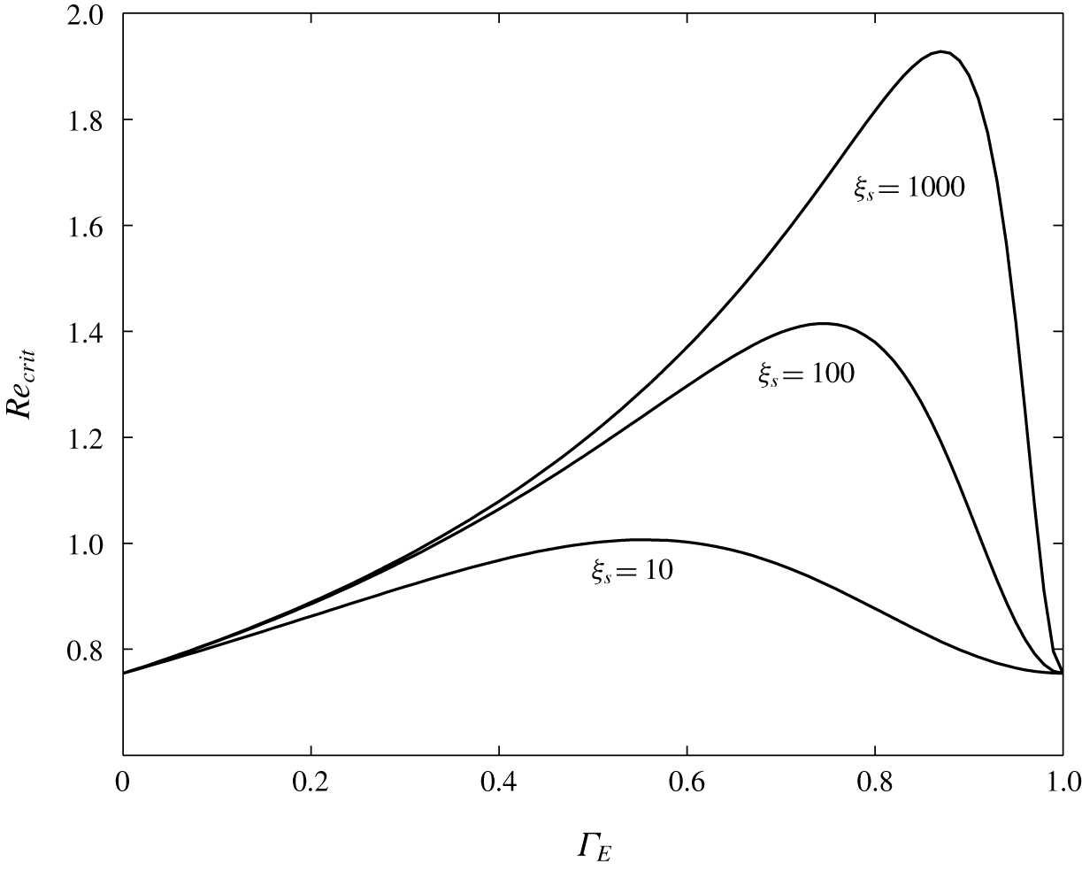
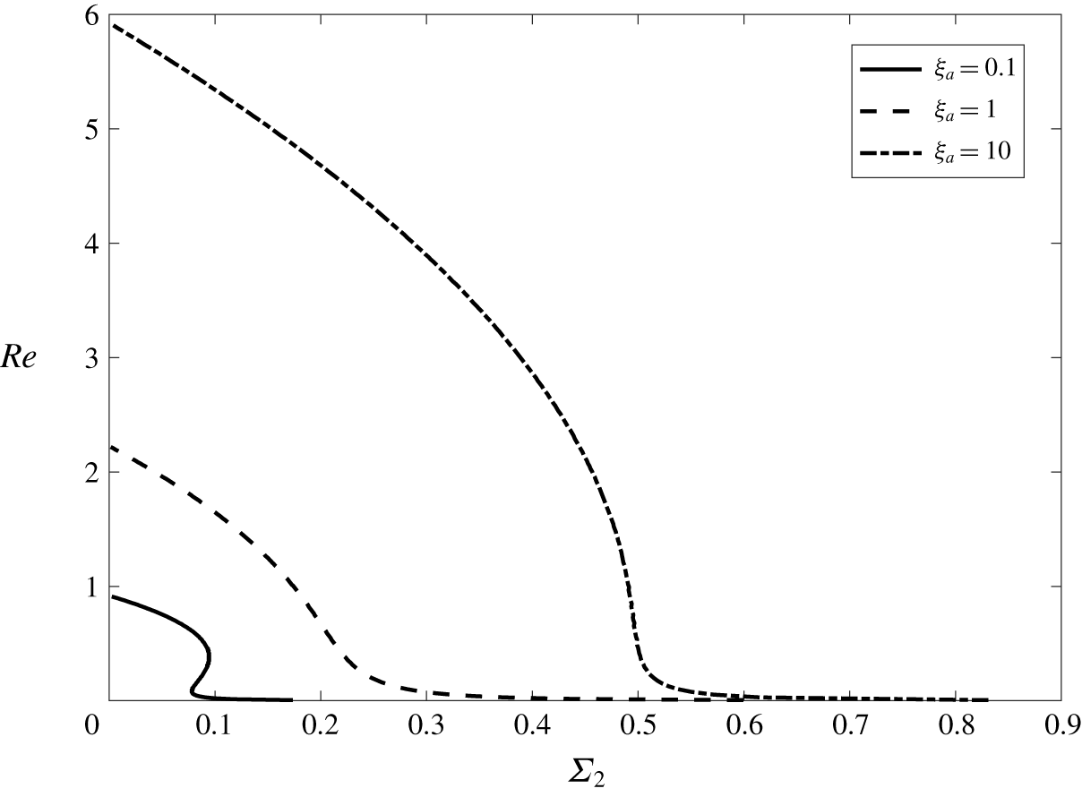
which is identical to the surfactant-free limit. Plotted in figure 2 are curves of  $Re_{crit}$ as a function of
 $\unicode[STIX]{x1D6E4}_{E}$ for various values of
 $\unicode[STIX]{x1D709}_{s}$. Lastly, expression (3.14) reproduces the familiar isothermal, surfactant-free case given by
 $Re_{crit}=5\cot \unicode[STIX]{x1D6FD}/6$ when
 $B=\unicode[STIX]{x1D6E4}_{E}=0$.
Value of  $Re_{crit}$ versus
 $\unicode[STIX]{x1D6E4}_{E}$ for various values of
 $\unicode[STIX]{x1D709}_{s}$ with
 $\cot \unicode[STIX]{x1D6FD}=M_{1}=M_{2}=B=1$.

We next present a physical mechanism responsible for the stability of the flow as was done by Wei (Reference Wei2005) for the insoluble surfactant model and by Karapetsas & Bontozoglou (Reference Karapetsas and Bontozoglou2014) for soluble surfactant case. We consider the flow rate given by
 $$\begin{eqnarray}q=\int _{0}^{1}(u_{E}+\tilde{u} )\,\text{d}z,\end{eqnarray}$$
with  $\tilde{u} (x,z,t)=\hat{u} (z)\tilde{h}(x,t)$. From the asymptotic analysis we find that
 $$\begin{eqnarray}q=1+\frac{3}{2}\tilde{h}+\text{i}kRe\tilde{h}\left(\frac{6}{5}-\frac{\cot \unicode[STIX]{x1D6FD}}{Re}+\frac{M_{2}B}{2(1+B)^{2}}-\frac{3M_{1}\unicode[STIX]{x1D6E4}_{E}\unicode[STIX]{x1D709}_{s}(1-\unicode[STIX]{x1D6E4}_{E})^{2}}{4+3\unicode[STIX]{x1D709}_{s}(1-\unicode[STIX]{x1D6E4}_{E})^{2}}\right)+O(k^{2}).\end{eqnarray}$$
We recognize that the quantity in the brackets will be zero for neutral stability and thus changes sign as we cross from a stable (negative) to an unstable (positive) configuration. To leading order  $q$ and
 $\tilde{h}$ are in phase, but as we learned from the asymptotic analysis the
 $O(k)$ problem determines the stability. For non-neutral cases the first-order problem reveals a phase shift of
 $\pm \unicode[STIX]{x03C0}/2$ between
 $q$ and
 $\tilde{h}$ where the sign corresponds to that of the quantity in the brackets. This phase shift is responsible for redistributing the fluid along the interface; when it is negative it has the effect of reducing the surface undulations and therefore stabilizes the flow, whereas when it is positive it causes fluid to pile up at the crest and in doing so destabilizes the flow. Now, the sign of the quantity in the brackets is influenced by the terms
 $$\begin{eqnarray}\frac{M_{2}B}{2(1+B)^{2}}\quad \text{and}\quad \frac{3M_{1}\unicode[STIX]{x1D6E4}_{E}\unicode[STIX]{x1D709}_{s}(1-\unicode[STIX]{x1D6E4}_{E})^{2}}{4+3\unicode[STIX]{x1D709}_{s}(1-\unicode[STIX]{x1D6E4}_{E})^{2}},\end{eqnarray}$$
which have opposite signs, and these competing influences will contribute to the overall stability.
3.2 Numerical solution
In this investigation we are primarily interested in the H and S modes. Although there is also a shear mode, it has been shown by Floryan, Davis & Kelly (Reference Floryan, Davis and Kelly1987) that this mode will only be important at small inclination angles, and hence we will focus on moderate inclination angles. The scaling that we have adopted in § 2 allowed us to obtain a nice simple relation for neutral stability and to analyse the H mode in detail. However, in order to capture the S mode we need to introduce a second scaling because the parameters involved in the neutral stability relation are in fact implicitly dependent on the Reynolds number. Thus, a rescaling of the problem must be considered which involves strictly independent parameters in order to ensure that all physical aspects are fully and correctly taken into account. For example, in the standard non-isothermal case involving the stability of a heated clean fluid, it is well known that a Marangoni number independent of  $Re$ must be introduced in order for the analysis to resolve the separate mode of instability which is entirely driven by thermocapillarity and stabilized by inertia (Kalliadasis et al. Reference Kalliadasis, Demekhin, Ruyer-Quil and Velarde2012). The new non-dimensional numbers can be expressed in terms of the parameters currently appearing in the neutral stability relation as
 $$\begin{eqnarray}\displaystyle & \displaystyle M_{1}=\left({\displaystyle \frac{3}{\sin \unicode[STIX]{x1D6FD}}}\right)^{1/3}\frac{Ka\unicode[STIX]{x1D6F4}_{1}}{Re^{5/3}(1-\unicode[STIX]{x1D6E4}_{E})},\quad M_{2}=-\left({\displaystyle \frac{3}{\sin \unicode[STIX]{x1D6FD}}}\right)^{1/3}\frac{Ka\unicode[STIX]{x1D6F4}_{2}}{Re^{5/3}}\ln (1-\unicode[STIX]{x1D6E4}_{E}) & \displaystyle \nonumber\\ \displaystyle & \displaystyle B=\left({\displaystyle \frac{3}{\sin \unicode[STIX]{x1D6FD}}}\right)^{1/3}Re^{1/3}Bi,\quad \unicode[STIX]{x1D709}_{s}=\left({\displaystyle \frac{\sin \unicode[STIX]{x1D6FD}}{3}}\right)^{1/3}{\displaystyle \frac{\unicode[STIX]{x1D709}_{a}}{Re^{1/3}}}, & \displaystyle \nonumber\end{eqnarray}$$
where the new parameters are the Kapitza number, given by  $Ka=\unicode[STIX]{x1D70E}_{p}(\unicode[STIX]{x1D70C}/\unicode[STIX]{x1D707}^{4}g)^{1/3}$, the solutal and thermal capillarity parameters given by
 $\unicode[STIX]{x1D6F4}_{1}=\unicode[STIX]{x1D6E4}_{\infty }RT_{a}/\unicode[STIX]{x1D70E}_{p}$ and
 $\unicode[STIX]{x1D6F4}_{2}=\unicode[STIX]{x1D6E4}_{\infty }R\unicode[STIX]{x0394}T/\unicode[STIX]{x1D70E}_{p}$, respectively, the rate of adsorption parameter
 $\unicode[STIX]{x1D709}_{a}=(g\unicode[STIX]{x1D70C}^{2}/\unicode[STIX]{x1D707}^{2})^{1/3}k_{1}/k_{2}$ and the Biot number
 $Bi=\unicode[STIX]{x1D6FC}_{g}/\unicode[STIX]{x1D70C}c_{p}\unicode[STIX]{x1D705}(\unicode[STIX]{x1D707}/\unicode[STIX]{x1D70C})^{2/3}g^{-1/3}$. Here, we have also incorporated the von Szyszkowski equation of state. We point out that in terms of these new parameters the neutral stability relation cannot be explicitly solved for the Reynolds number and the role played by the various physical factors cannot be clearly identified with separate terms as was done in (3.12). Shortly we will use this new relation to generate and interpret plots of neutral stability curves, but listing the formulation serves little purpose. Lastly, we must entertain the possibility that infinitely long perturbations are not the most unstable, in which case the neutral stability relation obtained from the asymptotic analysis does not accurately predict the threshold of instability for the equilibrium flow.
In order to determine the stability of perturbations of arbitrary wavenumber we employed a collocation method based on polynomial interpolation with Chebyshev points (Trefethen Reference Trefethen2000) to solve the eigenvalue problem (3.2)–(3.11). Accordingly, we introduced the expansions
 $$\begin{eqnarray}\unicode[STIX]{x1D6F9}=\mathop{\sum }_{j=0}^{N}w_{j}P_{j}(\unicode[STIX]{x1D709}),\quad {\hat{c}}=\mathop{\sum }_{j=0}^{N}v_{j}P_{j}(\unicode[STIX]{x1D709}),\quad \hat{T}=\mathop{\sum }_{j=0}^{N}\unicode[STIX]{x1D701}_{j}P_{j}(\unicode[STIX]{x1D709}),\end{eqnarray}$$
where  $\unicode[STIX]{x1D709}=2z-1$ and
 $$\begin{eqnarray}P_{j}(\unicode[STIX]{x1D709})=\frac{\displaystyle \mathop{\prod }_{\substack{ n=0 \\ n\neq j}}^{N}(\unicode[STIX]{x1D709}-\unicode[STIX]{x1D709}_{n})}{\displaystyle \mathop{\prod }_{\substack{ n=0 \\ n\neq j}}^{N}(\unicode[STIX]{x1D709}_{j}-\unicode[STIX]{x1D709}_{n})},\quad j=0,1,2,\ldots ,N,\end{eqnarray}$$
with  $\unicode[STIX]{x1D709}_{l}=-\cos (l\unicode[STIX]{x03C0}/N)$,
 $l=0,\;1,\;2,\ldots ,\;N$. This leads to an algebraic system of the form
 $$\begin{eqnarray}\boldsymbol{{\mathcal{A}}}y=v\boldsymbol{{\mathcal{B}}}y,\end{eqnarray}$$
where
 $$\begin{eqnarray}y=[w_{0}\;w_{1}\;\cdots \;w_{N}\;v_{0}\;v_{1}\;\cdots \;v_{N}\;\unicode[STIX]{x1D701}_{0}\;\unicode[STIX]{x1D701}_{1}\;\cdots \;\unicode[STIX]{x1D701}_{N}\;\unicode[STIX]{x1D702}\;\;\hat{\unicode[STIX]{x1D6E4}}]^{T},\end{eqnarray}$$
and  $\boldsymbol{{\mathcal{A}}}$ and
 $\boldsymbol{{\mathcal{B}}}$ are
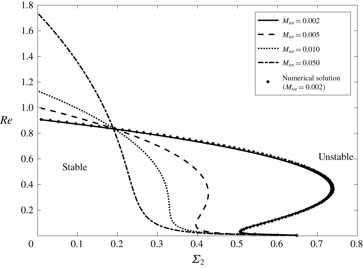
 $(3N+5)\times (3N+5)$ matrices. The eigenvalues of this system were calculated using the Matlab subroutine eig. The correct eigenvalue for the problem (3.2)–(3.11) was determined by recalculating the eigenvalues of the algebraic system for a finer grid and identifying the value that remained unchanged. The results from the collocation method confirm that the onset of instability in the equilibrium flow is in fact due to the amplification of infinitely long perturbations, and the critical conditions for instability are in excellent agreement with the predictions from the asymptotic analysis, as is illustrated in figure 3. This is similar to what is known to be the case for both isothermal flow with surfactants (Pascal et al. Reference Pascal, D’Alessio and Ellaban2019) and a clean fluid in a non-isothermal flow (Ellaban, Pascal & D’Alessio Reference Ellaban, Pascal and D’Alessio2017).
In presenting and interpreting our results we examine the stability map in the  $\unicode[STIX]{x1D6F4}_{2}Re$-plane. We plot the curves which denote the values of
 $Re$ and
 $\unicode[STIX]{x1D6F4}_{2}$ associated with neutral stability for the equilibrium flow. The region to the right of the neutral stability curve corresponds to instability, while for
 $Re$ and
 $\unicode[STIX]{x1D6F4}_{2}$ combinations in the region to the left the equilibrium flow is stable. As
 $\unicode[STIX]{x1D6F4}_{2}$ is the parameter measuring thermocapillarity, this observation is consistent with the destabilizing role played by the thermal Marangoni effect. There is also a critical level of thermocapillarity beyond which the flow is unstable for all Reynolds number. This is identified by the maximum
 $\unicode[STIX]{x1D6F4}_{2}$ value on the neutral stability curve. For lower values the flow is stable depending on the Reynolds number. For the basic non-isothermal flow of a clean fluid two separate modes of instability are known to exist: the so-called H mode which is driven by inertia and enhanced by thermocapillarity, hence distinguishable by the stability occurring as the Reynolds number is increased beyond a critical value, and the so-called S mode which is driven by thermocapillarity and impeded by inertia and occurring as the Reynolds number is decreased below a critical level.
Neutral stability curves for different values of  $M_{tot}$ in the
 $\unicode[STIX]{x1D6F4}_{2}Re$-plane with
 $\unicode[STIX]{x1D6F4}_{1}=0.07$,
 $\unicode[STIX]{x1D709}_{a}=1$,
 $Ka=3000$ and
 $Bi=1$.

In figure 3 we plot the neutral stability curves for different values of  $M_{tot}$ which measures the total concentration of surfactant added to the equilibrium flow. For one of the cases presented we also compare the numerical solution with that obtained by our asymptotic analysis and we see that the agreement is excellent. For small
 $\unicode[STIX]{x1D6F4}_{2}$ values (i.e. weak thermocapillarity) only the H mode is present. This is indicated by the fact that instability results as the Reynolds number is increased beyond the value for neutral stability, and it can be seen that the critical Reynolds number increases with
 $M_{tot}$. This behaviour is identical to isothermal flow for sufficiently low surfactant concentration, when adding a surfactant stabilizes the flow, as was explained above. However, for sufficiently large values of
 $\unicode[STIX]{x1D6F4}_{2}$ the region of stability shrinks as
 $M_{tot}$ is increased, meaning that adding more surfactant destabilizes the flow. As such, thermocapillarity effectuates a reversal in the stabilizing effect of surfactant doping. Now, the formula in (3.12) consists of separate terms for the solutal and thermal contributions to
 $Re_{crit}$, and therefore does not capture this coupling of the two effects. The explanation is the fact that the formula is in terms of the original parameters which are implicitly dependent on
 $Re_{crit}$, and it is thus evident that it is important to introduce the new parameters in order to accurately interpret the results.
Continuing with our examination of the results in figure 3 we see that for the smaller values of  $M_{tot}$, the curves clearly display the occurrence of both modes of instability for sufficiently large values of
 $\unicode[STIX]{x1D6F4}_{2}$. Specifically, for low Reynolds numbers the flow is unstable due to the S mode and for sufficiently high Reynolds numbers the H mode destabilizes the flow. The thresholds for the two modes are marked by two critical
 $Re$ values located on the neutral stability curve, with the interval between them corresponding to Reynolds numbers for which the flow is stable. It is interesting to note that adding surfactant stabilizes the flow for a narrow interval of small Reynolds numbers. Although the physical explanation for this is not clear, it is predicted by both our numerical and asymptotic results. As
 $M_{tot}$ is increased the S mode eventually disappears due to the rapid destabilization of the H mode which is triggered at significantly reduced levels of inertia. However, the thin region of stability next to the
 $Re=0$ axis persists and its extent with respect to
 $\unicode[STIX]{x1D6F4}_{2}$ values remains approximately fixed.
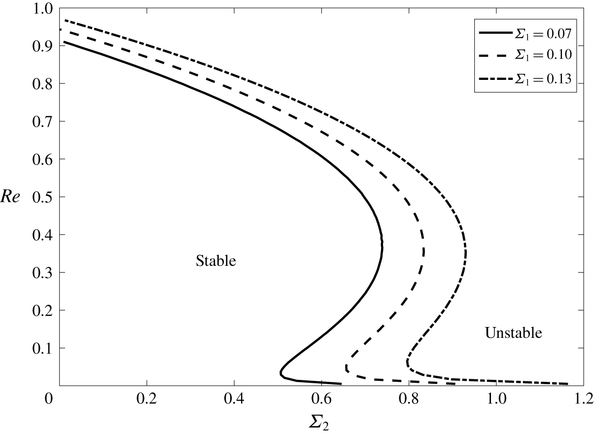
In the next set of results illustrated in figure 4 we show the effect of the parameter  $\unicode[STIX]{x1D6F4}_{1}$, which is related to the rate of variation in surface tension with respect to surfactant concentration. In determining a realistic range of values for this parameter we assumed that the value of the maximal surface concentration is
 $\unicode[STIX]{x1D6E4}_{\infty }=2\times 10^{-6}\,\text{mol}~\text{m}^{-2}$, as was done by Pereira & Kalliadasis (Reference Pereira and Kalliadasis2008). Then with
 $R=8.3145\,\text{N}~\text{m}~\text{mol}^{-1}~\text{K}^{-1}$ and
 $T_{a}=25\,^{\circ }\text{C}=298.15~\text{K}$, and using
 $\unicode[STIX]{x1D70E}_{p}=72\times 10^{-3}\,\text{N}~\text{m}^{-1}$ (the surface tension of water at
 $25\,^{\circ }\text{C}$) we obtain
 $\unicode[STIX]{x1D6F4}_{1}\approx 0.07$. It can be clearly seen that the region of stability increases with
 $\unicode[STIX]{x1D6F4}_{1}$ due to the stabilization of both the H and S modes. Since the rate of variation of surface tension with surfactant concentration is proportional to
 $\unicode[STIX]{x1D6F4}_{1}$, increasing this parameter strengthens the solutocapillary stresses which damp surface perturbations thus stabilizing the inertia-driven H mode. The fact that the S mode is stabilized indicates that solutocapillarity also counteracts the instability driven entirely by thermocapillarity.
Neutral stability curves for different values of  $\unicode[STIX]{x1D6F4}_{1}$ in the
 $\unicode[STIX]{x1D6F4}_{2}Re$-plane with
 $\unicode[STIX]{x1D709}_{a}=1$,
 $M_{tot}=0.002$,
 $Ka=3000$ and
 $Bi=1$.

Neutral stability curves for different values of  $\unicode[STIX]{x1D709}_{a}$ in the
 $\unicode[STIX]{x1D6F4}_{2}Re$-plane with
 $\unicode[STIX]{x1D6F4}_{1}=0.07$,
 $M_{tot}=0.1$,
 $Ka=3000$ and
 $Bi=1$.

Finally, in figure 5 we present the neutral stability curves for different values of  $\unicode[STIX]{x1D709}_{a}$. It is apparent that the region of stability increases with
 $\unicode[STIX]{x1D709}_{a}$, meaning that increasing surfactant solubility, which is associated with a decrease in
 $\unicode[STIX]{x1D709}_{a}$, destabilizes the flow regardless of the level of thermocapillarity. This behaviour is consistent with the fact that desorption of surfactant from the surface lowers concentration gradients along the surface and weakens the solutal Marangoni stresses.
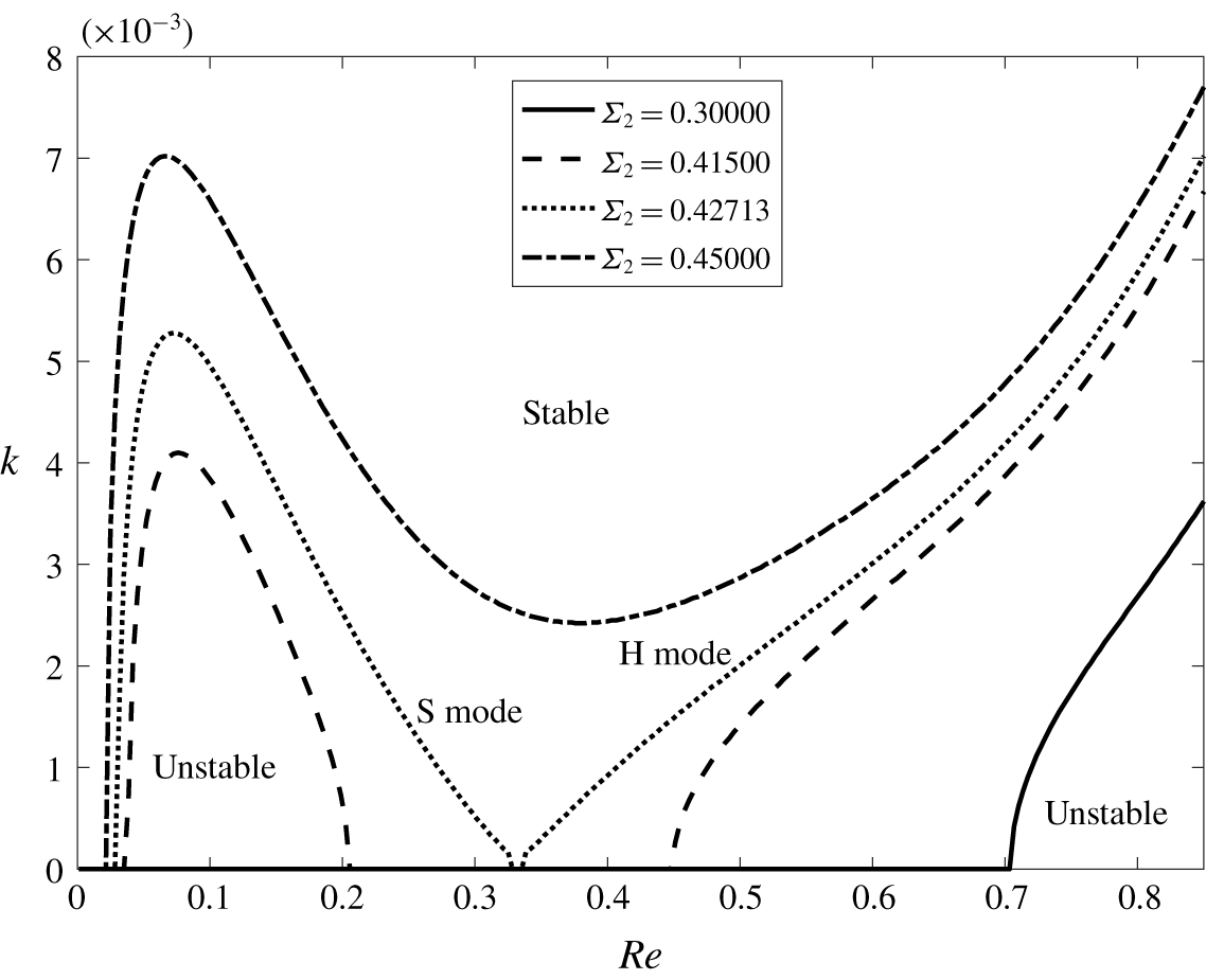
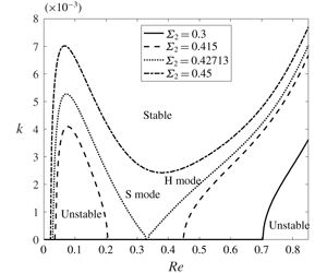
To complete our linear stability analysis we now consider the stability of different perturbation wavenumbers. This can be gauged from the results in figure 6 where we present the neutral stability curves in the  $Rek$-plane for different values of
 $\unicode[STIX]{x1D6F4}_{2}$ with
 $M_{tot}=0.005$, calculated using the numerical method. We first note that these results confirm that perturbations with
 $k=0$ are the most unstable as claimed above. Specifically, we see that the intervals of stable Reynolds numbers are narrowest for
 $k=0$ and widen as
 $k$ is increased. The intercepts of the curves with the
 $Re$ axis coincide with the critical Reynolds numbers for the onset of instability in the equilibrium flow at the specified
 $\unicode[STIX]{x1D6F4}_{2}$ values on the curve in figure 3 for
 $M_{tot}=0.005$. We also observe the merging of the H and S modes for
 $\unicode[STIX]{x1D6F4}_{2}=0.42713$. Also apparent in these results is that the shape of the S-mode branch of the curve is different from the one known to be obtained for a clean fluid. In that case
 $k$ decreases monotonically with
 $Re$ (Kalliadasis et al. Reference Kalliadasis, Demekhin, Ruyer-Quil and Velarde2012), while here it attains a maximum. In other words, for the basic non-isothermal flow, as
 $Re$ is decreased and inertia is lowered, more wavenumbers are destabilized by thermocapillarity. However, if surfactant is added a stabilizing effect takes place for very low Reynolds numbers and the range of unstable wavenumbers is reduced as
 $Re$ is decreased. Eventually all wavenumbers are stabilized resulting in a stable flow.
Neutral stability curves for different values of  $\unicode[STIX]{x1D6F4}_{2}$ in the
 $Rek$-plane with
 $M_{tot}=0.005$,
 $\unicode[STIX]{x1D6F4}_{1}=0.07$,
 $\unicode[STIX]{x1D709}_{a}=1$,
 $Ka=3000$,
 $Bi=1$,
 $Pr=7$,
 $Sc_{b}=Sc_{s}=700$ and
 $k_{d}=1$, where
 $Sc_{b}=\unicode[STIX]{x1D707}/\unicode[STIX]{x1D70C}D_{b}$,
 $Sc_{s}=\unicode[STIX]{x1D707}/\unicode[STIX]{x1D70C}D_{s}$ and
 $k_{d}=(\unicode[STIX]{x1D707}/g^{2}\unicode[STIX]{x1D70C})^{1/3}k_{2}$.

4 Nonlinear simulations
In this section we investigate the effect of nonlinearity on the stability of the flow. Since the S mode occurs at small Reynolds numbers and the weighted residual approximation is better suited to resolve the H mode at larger Reynolds numbers we revert back to the original scaling applied in § 2. We begin by introducing slow time ( $\unicode[STIX]{x1D70F}$) and space (
 $X$) variables and rescale the vertical velocity (
 $W$) according to
 $$\begin{eqnarray}\unicode[STIX]{x1D70F}=\unicode[STIX]{x1D700}t,\quad X=\unicode[STIX]{x1D700}x,\quad w=\unicode[STIX]{x1D700}W,\end{eqnarray}$$
where  $0<\unicode[STIX]{x1D700}\ll 1$ is a small parameter. Then the scaled governing equations (2.1)–(2.5) to second order in
 $\unicode[STIX]{x1D700}$ become
 $$\begin{eqnarray}\displaystyle & \displaystyle {\displaystyle \frac{\unicode[STIX]{x2202}u}{\unicode[STIX]{x2202}X}}+\frac{\unicode[STIX]{x2202}W}{\unicode[STIX]{x2202}z}=0, & \displaystyle\end{eqnarray}$$
 $$\begin{eqnarray}\displaystyle & \displaystyle \unicode[STIX]{x1D700}Re\left({\displaystyle \frac{\unicode[STIX]{x2202}u}{\unicode[STIX]{x2202}\unicode[STIX]{x1D70F}}}+u{\displaystyle \frac{\unicode[STIX]{x2202}u}{\unicode[STIX]{x2202}X}}+W{\displaystyle \frac{\unicode[STIX]{x2202}u}{\unicode[STIX]{x2202}z}}\right)=-\unicode[STIX]{x1D700}Re{\displaystyle \frac{\unicode[STIX]{x2202}p}{\unicode[STIX]{x2202}X}}+3+\unicode[STIX]{x1D700}^{2}{\displaystyle \frac{\unicode[STIX]{x2202}^{2}u}{\unicode[STIX]{x2202}X^{2}}}+{\displaystyle \frac{\unicode[STIX]{x2202}^{2}u}{\unicode[STIX]{x2202}z^{2}}}, & \displaystyle\end{eqnarray}$$
 $$\begin{eqnarray}\displaystyle & \displaystyle \unicode[STIX]{x1D700}^{2}Re\left({\displaystyle \frac{\unicode[STIX]{x2202}W}{\unicode[STIX]{x2202}\unicode[STIX]{x1D70F}}}+u{\displaystyle \frac{\unicode[STIX]{x2202}W}{\unicode[STIX]{x2202}X}}+W{\displaystyle \frac{\unicode[STIX]{x2202}W}{\unicode[STIX]{x2202}z}}\right)=-Re\frac{\unicode[STIX]{x2202}p}{\unicode[STIX]{x2202}z}-3\cot \unicode[STIX]{x1D6FD}+\unicode[STIX]{x1D700}{\displaystyle \frac{\unicode[STIX]{x2202}^{2}W}{\unicode[STIX]{x2202}z^{2}}}, & \displaystyle\end{eqnarray}$$
 $$\begin{eqnarray}\displaystyle & \displaystyle \unicode[STIX]{x1D700}Pe_{b}\left(\frac{\unicode[STIX]{x2202}c}{\unicode[STIX]{x2202}\unicode[STIX]{x1D70F}}+u{\displaystyle \frac{\unicode[STIX]{x2202}c}{\unicode[STIX]{x2202}X}}+W{\displaystyle \frac{\unicode[STIX]{x2202}c}{\unicode[STIX]{x2202}z}}\right)=\unicode[STIX]{x1D700}^{2}{\displaystyle \frac{\unicode[STIX]{x2202}^{2}c}{\unicode[STIX]{x2202}X^{2}}}+\frac{\unicode[STIX]{x2202}^{2}c}{\unicode[STIX]{x2202}z^{2}}, & \displaystyle\end{eqnarray}$$
 $$\begin{eqnarray}\displaystyle & \displaystyle \unicode[STIX]{x1D700}PrRe\left({\displaystyle \frac{\unicode[STIX]{x2202}T}{\unicode[STIX]{x2202}\unicode[STIX]{x1D70F}}}+u{\displaystyle \frac{\unicode[STIX]{x2202}T}{\unicode[STIX]{x2202}X}}+W{\displaystyle \frac{\unicode[STIX]{x2202}T}{\unicode[STIX]{x2202}z}}\right)=\unicode[STIX]{x1D700}^{2}{\displaystyle \frac{\unicode[STIX]{x2202}^{2}T}{\unicode[STIX]{x2202}X^{2}}}+{\displaystyle \frac{\unicode[STIX]{x2202}^{2}T}{\unicode[STIX]{x2202}z^{2}}}. & \displaystyle\end{eqnarray}$$
These can be viewed as the long-wave equations and mark the starting point of our nonlinear analysis.
Likewise, the transformed boundary conditions at  $z=h(X,\unicode[STIX]{x1D70F})$ to second order in
 $\unicode[STIX]{x1D700}$ are
 $$\begin{eqnarray}\displaystyle & \displaystyle p=\frac{2\unicode[STIX]{x1D700}}{Re}\left(\frac{\unicode[STIX]{x2202}W}{\unicode[STIX]{x2202}z}-\frac{\unicode[STIX]{x2202}h}{\unicode[STIX]{x2202}X}\frac{\unicode[STIX]{x2202}u}{\unicode[STIX]{x2202}z}\right)-\unicode[STIX]{x1D700}^{2}\left[We-M_{1}(\unicode[STIX]{x1D6E4}-\unicode[STIX]{x1D6E4}_{E})-M_{2}T\right]\frac{\unicode[STIX]{x2202}^{2}h}{\unicode[STIX]{x2202}X^{2}}, & \displaystyle\end{eqnarray}$$
 $$\begin{eqnarray}\displaystyle & \displaystyle W=\frac{\unicode[STIX]{x2202}h}{\unicode[STIX]{x2202}\unicode[STIX]{x1D70F}}+u\frac{\unicode[STIX]{x2202}h}{\unicode[STIX]{x2202}X}, & \displaystyle\end{eqnarray}$$
 $$\begin{eqnarray}\displaystyle & \displaystyle \unicode[STIX]{x1D700}\left(\frac{\unicode[STIX]{x2202}\unicode[STIX]{x1D6E4}}{\unicode[STIX]{x2202}\unicode[STIX]{x1D70F}}+u\frac{\unicode[STIX]{x2202}\unicode[STIX]{x1D6E4}}{\unicode[STIX]{x2202}X}\right)+\unicode[STIX]{x1D700}\unicode[STIX]{x1D6E4}\left(\frac{\unicode[STIX]{x2202}u}{\unicode[STIX]{x2202}X}+\frac{\unicode[STIX]{x2202}h}{\unicode[STIX]{x2202}X}\frac{\unicode[STIX]{x2202}u}{\unicode[STIX]{x2202}z}\right)=\frac{\unicode[STIX]{x1D700}^{2}}{Pe_{s}}\frac{\unicode[STIX]{x2202}^{2}\unicode[STIX]{x1D6E4}}{\unicode[STIX]{x2202}X^{2}}+k_{s}\left[\unicode[STIX]{x1D709}_{s}(1-\unicode[STIX]{x1D6E4})c-\unicode[STIX]{x1D6E4}\right], & \displaystyle\end{eqnarray}$$
 $$\begin{eqnarray}\displaystyle & \displaystyle \unicode[STIX]{x1D700}^{2}\frac{\unicode[STIX]{x2202}h}{\unicode[STIX]{x2202}X}\frac{\unicode[STIX]{x2202}c}{\unicode[STIX]{x2202}X}-\frac{\unicode[STIX]{x2202}c}{\unicode[STIX]{x2202}z}=Pe_{b}k_{s}\left[\unicode[STIX]{x1D709}_{s}(1-\unicode[STIX]{x1D6E4})c-\unicode[STIX]{x1D6E4}\right], & \displaystyle\end{eqnarray}$$
 $$\begin{eqnarray}\displaystyle & \displaystyle -\unicode[STIX]{x1D700}Re\left[M_{1}\frac{\unicode[STIX]{x2202}\unicode[STIX]{x1D6E4}}{\unicode[STIX]{x2202}X}+M_{2}\left(\frac{\unicode[STIX]{x2202}T}{\unicode[STIX]{x2202}X}+\frac{\unicode[STIX]{x2202}h}{\unicode[STIX]{x2202}X}\frac{\unicode[STIX]{x2202}T}{\unicode[STIX]{x2202}z}\right)\right]=\frac{\unicode[STIX]{x2202}u}{\unicode[STIX]{x2202}z}+\unicode[STIX]{x1D700}^{2}\frac{\unicode[STIX]{x2202}W}{\unicode[STIX]{x2202}X}-4\unicode[STIX]{x1D700}^{2}\frac{\unicode[STIX]{x2202}h}{\unicode[STIX]{x2202}X}\frac{\unicode[STIX]{x2202}u}{\unicode[STIX]{x2202}X}, & \displaystyle\end{eqnarray}$$
 $$\begin{eqnarray}\displaystyle & \displaystyle -BT=\frac{\unicode[STIX]{x2202}T}{\unicode[STIX]{x2202}z}-\unicode[STIX]{x1D700}^{2}\frac{\unicode[STIX]{x2202}h}{\unicode[STIX]{x2202}X}\frac{\unicode[STIX]{x2202}T}{\unicode[STIX]{x2202}X}, & \displaystyle\end{eqnarray}$$
while the bottom conditions at  $z=0$ are
 $$\begin{eqnarray}u=W=\frac{\unicode[STIX]{x2202}c}{\unicode[STIX]{x2202}z}=0,\quad T=1.\end{eqnarray}$$
4.1 Weighted residual model
We next implement a reduced model where the explicit dependence on the vertical coordinate is eliminated by applying a weighted residual technique. The method of weighted residuals was originally proposed by Ruyer-Quil & Manneville (Reference Ruyer-Quil and Manneville2000, Reference Ruyer-Quil and Manneville2002) to handle isothermal flows down an even incline. It has since been applied to more complicated flows (Kalliadasis et al. Reference Kalliadasis, Demekhin, Ruyer-Quil and Velarde2003a; D’Alessio, Pascal & Jasmine Reference D’Alessio, Pascal and Jasmine2009; Pascal & D’Alessio Reference Pascal and D’Alessio2010; D’Alessio et al. Reference D’Alessio, Pascal, Jasmine and Ogden2010; Ogden, D’Alessio & Pascal Reference Ogden, D’Alessio and Pascal2011; Pascal & D’Alessio Reference Pascal and D’Alessio2016; D’Alessio & Pascal Reference D’Alessio and Pascal2016; Ellaban et al. Reference Ellaban, Pascal and D’Alessio2017; Pascal, D’Alessio & Hasan Reference Pascal, D’Alessio and Hasan2018). Recently, Veremieiev & Wacks (Reference Veremieiev and Wacks2019) have extended the weighted residual method to include third- and fourth-order terms. Here, we extend the approach implemented by Pascal et al. (Reference Pascal, D’Alessio and Ellaban2019) to incorporate thermosoluto effects.
The basic idea behind the weighted residual method is to eliminate the  $z$ dependence by prescribing specific profiles for
 $u,T$ and
 $c$. We propose the following:
 $$\begin{eqnarray}\displaystyle & \displaystyle u=\frac{3q}{2h^{3}}b+\frac{\unicode[STIX]{x1D700}Re}{4h}\left(M_{1}\frac{\unicode[STIX]{x2202}\unicode[STIX]{x1D6E4}}{\unicode[STIX]{x2202}X}+M_{2}\frac{\unicode[STIX]{x2202}\unicode[STIX]{x1D703}}{\unicode[STIX]{x2202}X}\right)b_{1}, & \displaystyle \nonumber\\ \displaystyle & \displaystyle T=1+\frac{(\unicode[STIX]{x1D703}-1)}{h}z, & \displaystyle \nonumber\\ \displaystyle & \displaystyle c=C+\frac{Pe_{b}k_{s}}{2h}\left[\unicode[STIX]{x1D709}_{s}(1-\unicode[STIX]{x1D6E4})C-\unicode[STIX]{x1D6E4}\right](h^{2}-z^{2}), & \displaystyle \nonumber\end{eqnarray}$$
where  $b$ and
 $b_{1}$ are given by
 $$\begin{eqnarray}b=z(2h-z),\quad b_{1}=z(2h-3z).\end{eqnarray}$$
We note that the proposed profile for  $T$ represents a linear variation in temperature with respect to
 $z$, while that for
 $c$ corresponds to a linear variation in the gradient
 $\unicode[STIX]{x2202}c/\unicode[STIX]{x2202}z$ with respect to
 $z$. Here,
 $C(X,\unicode[STIX]{x1D70F})=c(X,z=h,\unicode[STIX]{x1D70F})$ denotes the bulk concentration at the interface, whereas
 $\unicode[STIX]{x1D703}(X,\unicode[STIX]{x1D70F})=T(X,z=h,\unicode[STIX]{x1D70F})$ is the surface temperature, and
 $$\begin{eqnarray}q=\int _{0}^{h}u\,\text{d}z,\end{eqnarray}$$
is the flow rate. We point out that the profiles for  $u$ and
 $c$ satisfy all the boundary conditions including the free-surface conditions to
 $O(\unicode[STIX]{x1D700}^{2})$. Although the profile for
 $T$ satisfies the bottom condition, it does not satisfy the free-surface condition. In fact, it is impossible for the profile to satisfy both. However, as explained by Kalliadasis et al. (Reference Kalliadasis, Demekhin, Ruyer-Quil and Velarde2003a), the free-surface condition is incorporated into the energy equation when it is integrated over the fluid thickness, as described below. The profiles for
 $u$ and
 $T$ have been used in previous studies, whereas the particular choice for
 $c$ is new and an explanation behind this choice is given in appendix A.
In accordance with the Galerkin approach we take  $b$ as the weight function and multiply (4.2) by
 $b$ and integrate with respect to
 $z$ from
 $0$ to
 $h$. The pressure term in (4.2) is eliminated by using (4.3) as follows. First, we discard the
 $O(\unicode[STIX]{x1D700}^{2})$ terms to obtain
 $$\begin{eqnarray}\frac{\unicode[STIX]{x2202}p}{\unicode[STIX]{x2202}z}=-\frac{3\cot \unicode[STIX]{x1D6FD}}{Re}+\frac{\unicode[STIX]{x1D700}}{Re}\frac{\unicode[STIX]{x2202}^{2}W}{\unicode[STIX]{x2202}z^{2}}.\end{eqnarray}$$
This is then integrated from  $z$ to
 $h$ and the boundary condition (4.6) at
 $z=h$ is applied to yield an expression for the pressure which is then substituted into (4.2). Since the pressure term is multiplied by
 $\unicode[STIX]{x1D700}$ in (4.2), the
 $O(\unicode[STIX]{x1D700}^{2})$ terms in (4.3) can be ignored. This will result in a second-order weighted residual model. For the concentration equation we take the weight function to be unity and integrate from
 $z=0$ to
 $z=h$, while for the energy equation we choose
 $z$ as the weight function and integrate over the liquid layer. After some algebra we obtain the following second-order equations for the flow variables
 $h,q,\unicode[STIX]{x1D719}=h(\unicode[STIX]{x1D703}-1),\unicode[STIX]{x1D712}=h^{2}[\unicode[STIX]{x1D709}_{s}(1-\unicode[STIX]{x1D6E4})C-\unicode[STIX]{x1D6E4}]$ and
 $\unicode[STIX]{x1D6E4}$
 $$\begin{eqnarray}\frac{\unicode[STIX]{x2202}h}{\unicode[STIX]{x2202}\unicode[STIX]{x1D70F}}+\frac{\unicode[STIX]{x2202}q}{\unicode[STIX]{x2202}X}=0,\end{eqnarray}$$
 $$\begin{eqnarray}\displaystyle & & \displaystyle \displaystyle \frac{\unicode[STIX]{x2202}q}{\unicode[STIX]{x2202}\unicode[STIX]{x1D70F}}+\frac{\unicode[STIX]{x2202}}{\unicode[STIX]{x2202}X}\left[\frac{9}{7}\frac{q^{2}}{h}+\frac{5\cot \unicode[STIX]{x1D6FD}}{4Re}h^{2}+\frac{5M_{1}}{4}\unicode[STIX]{x1D6E4}+\frac{5M_{2}}{4}\frac{\unicode[STIX]{x1D719}}{h}\right]=\frac{q}{7h}\frac{\unicode[STIX]{x2202}q}{\unicode[STIX]{x2202}X}+\frac{5}{2\unicode[STIX]{x1D700}Re}\left(h-\frac{q}{h^{2}}\right)\nonumber\\ \displaystyle & & \displaystyle \qquad +\,\frac{\unicode[STIX]{x1D700}}{Re}\left[\frac{9}{2}\frac{\unicode[STIX]{x2202}^{2}q}{\unicode[STIX]{x2202}X^{2}}-\frac{9}{2h}\frac{\unicode[STIX]{x2202}h}{\unicode[STIX]{x2202}X}\frac{\unicode[STIX]{x2202}q}{\unicode[STIX]{x2202}X}+\frac{4q}{h^{2}}\left(\frac{\unicode[STIX]{x2202}h}{\unicode[STIX]{x2202}X}\right)^{2}-\frac{6q}{h}\frac{\unicode[STIX]{x2202}^{2}h}{\unicode[STIX]{x2202}X^{2}}\right]\nonumber\\ \displaystyle & & \displaystyle \qquad +\,\frac{\unicode[STIX]{x1D700}M_{1}Re}{16}\left[\frac{h^{2}}{3}\frac{\unicode[STIX]{x2202}^{2}\unicode[STIX]{x1D6E4}}{\unicode[STIX]{x2202}X\unicode[STIX]{x2202}\unicode[STIX]{x1D70F}}+\frac{15hq}{14}\frac{\unicode[STIX]{x2202}^{2}\unicode[STIX]{x1D6E4}}{\unicode[STIX]{x2202}X^{2}}+\frac{19h}{21}\frac{\unicode[STIX]{x2202}\unicode[STIX]{x1D6E4}}{\unicode[STIX]{x2202}X}\frac{\unicode[STIX]{x2202}q}{\unicode[STIX]{x2202}X}+\frac{5q}{7}\frac{\unicode[STIX]{x2202}h}{\unicode[STIX]{x2202}X}\frac{\unicode[STIX]{x2202}\unicode[STIX]{x1D6E4}}{\unicode[STIX]{x2202}X}\right]\nonumber\\ \displaystyle & & \displaystyle \qquad +\,\frac{\unicode[STIX]{x1D700}M_{2}Re}{16}\left[\frac{h}{3}\frac{\unicode[STIX]{x2202}^{2}\unicode[STIX]{x1D719}}{\unicode[STIX]{x2202}X\unicode[STIX]{x2202}\unicode[STIX]{x1D70F}}-\frac{1}{3}\frac{\unicode[STIX]{x2202}h}{\unicode[STIX]{x2202}X}\frac{\unicode[STIX]{x2202}\unicode[STIX]{x1D719}}{\unicode[STIX]{x2202}\unicode[STIX]{x1D70F}}+\frac{26}{21}\frac{\unicode[STIX]{x2202}\unicode[STIX]{x1D719}}{\unicode[STIX]{x2202}X}\frac{\unicode[STIX]{x2202}q}{\unicode[STIX]{x2202}X}-\frac{11\unicode[STIX]{x1D719}}{7h}\frac{\unicode[STIX]{x2202}h}{\unicode[STIX]{x2202}X}\frac{\unicode[STIX]{x2202}q}{\unicode[STIX]{x2202}X}+\frac{\unicode[STIX]{x1D719}}{3}\frac{\unicode[STIX]{x2202}^{2}q}{\unicode[STIX]{x2202}X^{2}}\right.\nonumber\\ \displaystyle & & \displaystyle \qquad \left.+\frac{15q}{14}\frac{\unicode[STIX]{x2202}^{2}\unicode[STIX]{x1D719}}{\unicode[STIX]{x2202}X^{2}}-\frac{10q}{7h}\frac{\unicode[STIX]{x2202}h}{\unicode[STIX]{x2202}X}\frac{\unicode[STIX]{x2202}\unicode[STIX]{x1D719}}{\unicode[STIX]{x2202}X}+\frac{10q\unicode[STIX]{x1D719}}{7h^{2}}\left(\frac{\unicode[STIX]{x2202}h}{\unicode[STIX]{x2202}X}\right)^{2}-\frac{15q\unicode[STIX]{x1D719}}{14h}\frac{\unicode[STIX]{x2202}^{2}h}{\unicode[STIX]{x2202}X^{2}}\right],\end{eqnarray}$$
 $$\begin{eqnarray}\displaystyle & & \displaystyle \displaystyle \frac{\unicode[STIX]{x2202}\unicode[STIX]{x1D719}}{\unicode[STIX]{x2202}\unicode[STIX]{x1D70F}}+\frac{\unicode[STIX]{x2202}}{\unicode[STIX]{x2202}X}\left[\frac{27}{20}\frac{q\unicode[STIX]{x1D719}}{h}\right]=\frac{7\unicode[STIX]{x1D719}}{40h}\frac{\unicode[STIX]{x2202}q}{\unicode[STIX]{x2202}X}-\frac{3}{\unicode[STIX]{x1D700}PrReh}\left[B(h+\unicode[STIX]{x1D719})+\frac{\unicode[STIX]{x1D719}}{h}\right]\nonumber\\ \displaystyle & & \displaystyle \quad +\,\frac{3\unicode[STIX]{x1D700}M_{1}Re}{80}\left[h\unicode[STIX]{x1D719}\frac{\unicode[STIX]{x2202}^{2}\unicode[STIX]{x1D6E4}}{\unicode[STIX]{x2202}X^{2}}+2h\frac{\unicode[STIX]{x2202}\unicode[STIX]{x1D719}}{\unicode[STIX]{x2202}X}\frac{\unicode[STIX]{x2202}\unicode[STIX]{x1D6E4}}{\unicode[STIX]{x2202}X}\right]\nonumber\\ \displaystyle & & \displaystyle \quad +\,\frac{\unicode[STIX]{x1D700}}{PrRe}\left[\frac{\unicode[STIX]{x2202}^{2}\unicode[STIX]{x1D719}}{\unicode[STIX]{x2202}X^{2}}-\frac{1}{h}\frac{\unicode[STIX]{x2202}h}{\unicode[STIX]{x2202}X}\frac{\unicode[STIX]{x2202}\unicode[STIX]{x1D719}}{\unicode[STIX]{x2202}X}-\frac{2\unicode[STIX]{x1D719}}{h}\frac{\unicode[STIX]{x2202}^{2}h}{\unicode[STIX]{x2202}X^{2}}-\frac{3B}{2}\left(1+\frac{\unicode[STIX]{x1D719}}{h}\right)\left(\frac{\unicode[STIX]{x2202}h}{\unicode[STIX]{x2202}X}\right)^{2}\right]\nonumber\\ \displaystyle & & \displaystyle \quad +\frac{3\unicode[STIX]{x1D700}M_{2}Re}{80}\left[\unicode[STIX]{x1D719}\frac{\unicode[STIX]{x2202}^{2}\unicode[STIX]{x1D719}}{\unicode[STIX]{x2202}X^{2}}+2\left(\frac{\unicode[STIX]{x2202}\unicode[STIX]{x1D719}}{\unicode[STIX]{x2202}X}\right)^{2}-\frac{4\unicode[STIX]{x1D719}}{h}\frac{\unicode[STIX]{x2202}h}{\unicode[STIX]{x2202}X}\frac{\unicode[STIX]{x2202}\unicode[STIX]{x1D719}}{\unicode[STIX]{x2202}X}-\frac{\unicode[STIX]{x1D719}^{2}}{h}\frac{\unicode[STIX]{x2202}^{2}h}{\unicode[STIX]{x2202}X^{2}}+\frac{2\unicode[STIX]{x1D719}^{2}}{h^{2}}\left(\frac{\unicode[STIX]{x2202}h}{\unicode[STIX]{x2202}X}\right)^{2}\right],\quad\end{eqnarray}$$
 $$\begin{eqnarray}\displaystyle & & \displaystyle \displaystyle \frac{\unicode[STIX]{x2202}}{\unicode[STIX]{x2202}\unicode[STIX]{x1D70F}}\left(\unicode[STIX]{x1D712}+\frac{3hC}{Pe_{b}k_{s}}\right)+\frac{\unicode[STIX]{x2202}}{\unicode[STIX]{x2202}X}\left[\frac{33}{40}\frac{q\unicode[STIX]{x1D712}}{h}+\frac{3qC}{Pe_{b}k_{s}}\right]\nonumber\\ \displaystyle & & \displaystyle \quad \displaystyle =\frac{\unicode[STIX]{x1D700}}{Pe_{b}}\left[\frac{\unicode[STIX]{x2202}^{2}\unicode[STIX]{x1D712}}{\unicode[STIX]{x2202}X^{2}}-\frac{3\unicode[STIX]{x1D712}}{h^{2}}\left(\frac{\unicode[STIX]{x2202}h}{\unicode[STIX]{x2202}X}\right)^{2}\right]-\frac{3}{\unicode[STIX]{x1D700}Pe_{b}}\frac{\unicode[STIX]{x1D712}}{h^{2}}+\frac{3\unicode[STIX]{x1D700}h}{Pe_{b}^{2}k_{s}}\frac{\unicode[STIX]{x2202}^{2}C}{\unicode[STIX]{x2202}X^{2}}\nonumber\\ \displaystyle & & \displaystyle \qquad -\,\frac{3\unicode[STIX]{x1D700}Re}{80}\left[h\unicode[STIX]{x1D712}\left(M_{1}\frac{\unicode[STIX]{x2202}^{2}\unicode[STIX]{x1D6E4}}{\unicode[STIX]{x2202}X^{2}}+\frac{M_{2}}{h}\left\{\frac{\unicode[STIX]{x2202}^{2}\unicode[STIX]{x1D719}}{\unicode[STIX]{x2202}X^{2}}-\frac{2}{h}\frac{\unicode[STIX]{x2202}h}{\unicode[STIX]{x2202}X}\frac{\unicode[STIX]{x2202}\unicode[STIX]{x1D719}}{\unicode[STIX]{x2202}X}-\frac{\unicode[STIX]{x1D719}}{h}\frac{\unicode[STIX]{x2202}^{2}h}{\unicode[STIX]{x2202}X^{2}}+\frac{2\unicode[STIX]{x1D719}}{h^{2}}\left(\frac{\unicode[STIX]{x2202}h}{\unicode[STIX]{x2202}X}\right)^{2}\right\}\right)\right.\nonumber\\ \displaystyle & & \displaystyle \qquad +\,\frac{\unicode[STIX]{x2202}\unicode[STIX]{x1D712}}{\unicode[STIX]{x2202}X}\left(M_{1}h\frac{\unicode[STIX]{x2202}\unicode[STIX]{x1D6E4}}{\unicode[STIX]{x2202}X}+M_{2}\left\{\frac{\unicode[STIX]{x2202}\unicode[STIX]{x1D719}}{\unicode[STIX]{x2202}X}-\frac{\unicode[STIX]{x1D719}}{h}\frac{\unicode[STIX]{x2202}h}{\unicode[STIX]{x2202}X}\right\}\right)\nonumber\\ \displaystyle & & \displaystyle \qquad \left.+\,\unicode[STIX]{x1D712}\frac{\unicode[STIX]{x2202}h}{\unicode[STIX]{x2202}X}\left(M_{1}\frac{\unicode[STIX]{x2202}\unicode[STIX]{x1D6E4}}{\unicode[STIX]{x2202}X}+\frac{M_{2}}{h}\left\{\frac{\unicode[STIX]{x2202}\unicode[STIX]{x1D719}}{\unicode[STIX]{x2202}X}-\frac{\unicode[STIX]{x1D719}}{h}\frac{\unicode[STIX]{x2202}h}{\unicode[STIX]{x2202}X}\right\}\right)\right].\end{eqnarray}$$
 $$\begin{eqnarray}\displaystyle & & \displaystyle \frac{\unicode[STIX]{x2202}\unicode[STIX]{x1D6E4}}{\unicode[STIX]{x2202}\unicode[STIX]{x1D70F}}+\frac{\unicode[STIX]{x2202}}{\unicode[STIX]{x2202}X}\left[\frac{3}{2}\frac{q\unicode[STIX]{x1D6E4}}{h}\right]=\frac{\unicode[STIX]{x1D700}}{Pe_{s}}\frac{\unicode[STIX]{x2202}^{2}\unicode[STIX]{x1D6E4}}{\unicode[STIX]{x2202}X^{2}}+\unicode[STIX]{x1D700}Re\unicode[STIX]{x1D6E4}\frac{\unicode[STIX]{x2202}h}{\unicode[STIX]{x2202}X}\left[M_{1}\frac{\unicode[STIX]{x2202}\unicode[STIX]{x1D6E4}}{\unicode[STIX]{x2202}X}+\frac{M_{2}}{h}\left(\frac{\unicode[STIX]{x2202}\unicode[STIX]{x1D719}}{\unicode[STIX]{x2202}X}-\frac{\unicode[STIX]{x1D719}}{h}\frac{\unicode[STIX]{x2202}h}{\unicode[STIX]{x2202}X}\right)\right]+\frac{k_{s}}{\unicode[STIX]{x1D700}}\frac{\unicode[STIX]{x1D712}}{h^{2}}\nonumber\\ \displaystyle & & \displaystyle \qquad +\,\frac{\unicode[STIX]{x1D700}Re}{4}\left[h\unicode[STIX]{x1D6E4}\left(M_{1}\frac{\unicode[STIX]{x2202}^{2}\unicode[STIX]{x1D6E4}}{\unicode[STIX]{x2202}X^{2}}+\frac{M_{2}}{h}\left\{\frac{\unicode[STIX]{x2202}^{2}\unicode[STIX]{x1D719}}{\unicode[STIX]{x2202}X^{2}}-\frac{2}{h}\frac{\unicode[STIX]{x2202}h}{\unicode[STIX]{x2202}X}\frac{\unicode[STIX]{x2202}\unicode[STIX]{x1D719}}{\unicode[STIX]{x2202}X}-\frac{\unicode[STIX]{x1D719}}{h}\frac{\unicode[STIX]{x2202}^{2}h}{\unicode[STIX]{x2202}X^{2}}+\frac{2\unicode[STIX]{x1D719}}{h^{2}}\left(\frac{\unicode[STIX]{x2202}h}{\unicode[STIX]{x2202}X}\right)^{2}\right\}\right)\right.\nonumber\\ \displaystyle & & \displaystyle \qquad +\,\frac{\unicode[STIX]{x2202}\unicode[STIX]{x1D6E4}}{\unicode[STIX]{x2202}X}\left(M_{1}h\frac{\unicode[STIX]{x2202}\unicode[STIX]{x1D6E4}}{\unicode[STIX]{x2202}X}+M_{2}\left\{\frac{\unicode[STIX]{x2202}\unicode[STIX]{x1D719}}{\unicode[STIX]{x2202}X}-\frac{\unicode[STIX]{x1D719}}{h}\frac{\unicode[STIX]{x2202}h}{\unicode[STIX]{x2202}X}\right\}\right)\nonumber\\ \displaystyle & & \displaystyle \qquad \left.+\,\unicode[STIX]{x1D6E4}\frac{\unicode[STIX]{x2202}h}{\unicode[STIX]{x2202}X}\left(M_{1}\frac{\unicode[STIX]{x2202}\unicode[STIX]{x1D6E4}}{\unicode[STIX]{x2202}X}+\frac{M_{2}}{h}\left\{\frac{\unicode[STIX]{x2202}\unicode[STIX]{x1D719}}{\unicode[STIX]{x2202}X}-\frac{\unicode[STIX]{x1D719}}{h}\frac{\unicode[STIX]{x2202}h}{\unicode[STIX]{x2202}X}\right\}\right)\right].\end{eqnarray}$$
As a check, we carried out a linear stability analysis on the above system and were able to reproduce the expression for the critical Reynolds number given by (3.14).
To numerically solve the system of (4.13)–(4.17) we first express these equations in the form
 $$\begin{eqnarray}\displaystyle & \displaystyle \frac{\unicode[STIX]{x2202}h}{\unicode[STIX]{x2202}\unicode[STIX]{x1D70F}}+\frac{\unicode[STIX]{x2202}q}{\unicode[STIX]{x2202}X}=0, & \displaystyle \nonumber\\ \displaystyle & \displaystyle \frac{\unicode[STIX]{x2202}q}{\unicode[STIX]{x2202}\unicode[STIX]{x1D70F}}+\frac{\unicode[STIX]{x2202}}{\unicode[STIX]{x2202}X}\left[\frac{9}{7}\frac{q^{2}}{h}+\frac{5\cot \unicode[STIX]{x1D6FD}}{4Re}h^{2}+\frac{5M_{1}}{4}\unicode[STIX]{x1D6E4}+\frac{5M_{2}}{4}\frac{\unicode[STIX]{x1D719}}{h}\right]=S_{1}+Q_{1}, & \displaystyle \nonumber\\ \displaystyle & \displaystyle \frac{\unicode[STIX]{x2202}\unicode[STIX]{x1D719}}{\unicode[STIX]{x2202}\unicode[STIX]{x1D70F}}+\frac{\unicode[STIX]{x2202}}{\unicode[STIX]{x2202}X}\left[\frac{27}{20}\frac{q\unicode[STIX]{x1D719}}{h}\right]=S_{2}+Q_{2}, & \displaystyle \nonumber\\ \displaystyle & \displaystyle \frac{\unicode[STIX]{x2202}\unicode[STIX]{x1D712}}{\unicode[STIX]{x2202}\unicode[STIX]{x1D70F}}+\frac{\unicode[STIX]{x2202}}{\unicode[STIX]{x2202}X}\left[\frac{33}{40}\frac{q\unicode[STIX]{x1D712}}{h}\right]=S_{3}+Q_{3}, & \displaystyle \nonumber\\ \displaystyle & \displaystyle \frac{\unicode[STIX]{x2202}\unicode[STIX]{x1D6E4}}{\unicode[STIX]{x2202}\unicode[STIX]{x1D70F}}+\frac{\unicode[STIX]{x2202}}{\unicode[STIX]{x2202}X}\left[\frac{3}{2}\frac{q\unicode[STIX]{x1D6E4}}{h}\right]=S_{4}+Q_{4}, & \displaystyle \nonumber\end{eqnarray}$$
where the gradient-free source terms  $S_{1},S_{2},S_{3}$ are given by
 $$\begin{eqnarray}S_{1}=\frac{5}{2\unicode[STIX]{x1D700}Re}\!\left(h-\frac{q}{h^{2}}\right),\quad S_{2}=-\frac{3}{\unicode[STIX]{x1D700}PrReh}\!\left[B(h+\unicode[STIX]{x1D719})+\frac{\unicode[STIX]{x1D719}}{h}\right],\quad S_{3}=-\frac{3}{\unicode[STIX]{x1D700}Pe_{b}}\frac{\unicode[STIX]{x1D712}}{h^{2}},\quad S_{4}=\frac{k_{s}}{\unicode[STIX]{x1D700}}\frac{\unicode[STIX]{x1D712}}{h^{2}},\end{eqnarray}$$
and  $Q_{1},Q_{2},Q_{3},Q_{4}$ can be easily determined from (4.14)–(4.17), respectively. To solve this system of equations the fractional-step splitting technique (Leveque Reference Leveque2002) was implemented. We first solve
 $$\begin{eqnarray}\displaystyle & \displaystyle \frac{\unicode[STIX]{x2202}h}{\unicode[STIX]{x2202}\unicode[STIX]{x1D70F}}+\frac{\unicode[STIX]{x2202}q}{\unicode[STIX]{x2202}X}=0, & \displaystyle \nonumber\\ \displaystyle & \displaystyle \frac{\unicode[STIX]{x2202}q}{\unicode[STIX]{x2202}\unicode[STIX]{x1D70F}}+\frac{\unicode[STIX]{x2202}}{\unicode[STIX]{x2202}X}\left[\frac{9}{7}\frac{q^{2}}{h}+\frac{5\cot \unicode[STIX]{x1D6FD}}{4Re}h^{2}+\frac{5M_{1}}{4}\unicode[STIX]{x1D6E4}+\frac{5M_{2}}{4}\frac{\unicode[STIX]{x1D719}}{h}\right]=S_{1}, & \displaystyle \nonumber\\ \displaystyle & \displaystyle \frac{\unicode[STIX]{x2202}\unicode[STIX]{x1D719}}{\unicode[STIX]{x2202}\unicode[STIX]{x1D70F}}+\frac{\unicode[STIX]{x2202}}{\unicode[STIX]{x2202}X}\left[\frac{27}{20}\frac{q\unicode[STIX]{x1D719}}{h}\right]=S_{2}, & \displaystyle \nonumber\\ \displaystyle & \displaystyle \frac{\unicode[STIX]{x2202}\unicode[STIX]{x1D712}}{\unicode[STIX]{x2202}\unicode[STIX]{x1D70F}}+\frac{\unicode[STIX]{x2202}}{\unicode[STIX]{x2202}X}\left[\frac{33}{40}\frac{q\unicode[STIX]{x1D712}}{h}\right]=S_{3}, & \displaystyle \nonumber\\ \displaystyle & \displaystyle \frac{\unicode[STIX]{x2202}\unicode[STIX]{x1D6E4}}{\unicode[STIX]{x2202}\unicode[STIX]{x1D70F}}+\frac{\unicode[STIX]{x2202}}{\unicode[STIX]{x2202}X}\left[\frac{3}{2}\frac{q\unicode[STIX]{x1D6E4}}{h}\right]=S_{4}, & \displaystyle \nonumber\end{eqnarray}$$
over a time step  $\unicode[STIX]{x0394}\unicode[STIX]{x1D70F}$, and then solve
 $$\begin{eqnarray}\frac{\unicode[STIX]{x2202}q}{\unicode[STIX]{x2202}\unicode[STIX]{x1D70F}}=Q_{1},\quad \frac{\unicode[STIX]{x2202}\unicode[STIX]{x1D719}}{\unicode[STIX]{x2202}\unicode[STIX]{x1D70F}}=Q_{2},\quad \frac{\unicode[STIX]{x2202}\unicode[STIX]{x1D712}}{\unicode[STIX]{x2202}\unicode[STIX]{x1D70F}}=Q_{3},\quad \frac{\unicode[STIX]{x2202}\unicode[STIX]{x1D6E4}}{\unicode[STIX]{x2202}\unicode[STIX]{x1D70F}}=Q_{4},\end{eqnarray}$$
using the solution obtained from the first step as an initial condition for the second step. The second step then returns the solution for  $q,\unicode[STIX]{x1D6E4},\unicode[STIX]{x1D712}$ at the new time
 $\unicode[STIX]{x1D70F}+\unicode[STIX]{x0394}\unicode[STIX]{x1D70F}$.
The first step involves solving a nonlinear system of hyperbolic conservation laws which, when expressed in vector form, can be written compactly as
 $$\begin{eqnarray}\frac{\unicode[STIX]{x2202}\boldsymbol{U}}{\unicode[STIX]{x2202}\unicode[STIX]{x1D70F}}+\frac{\unicode[STIX]{x2202}\boldsymbol{F}(\boldsymbol{U})}{\unicode[STIX]{x2202}X}=\boldsymbol{B}(\boldsymbol{U}),\end{eqnarray}$$
where
 $$\begin{eqnarray}\boldsymbol{U}=\left[\begin{array}{@{}c@{}}h\\ q\\ \unicode[STIX]{x1D719}\\ \unicode[STIX]{x1D712}\\ \unicode[STIX]{x1D6E4}\end{array}\right],\quad \boldsymbol{F}(\boldsymbol{U})=\left[\begin{array}{@{}c@{}}q\\ {\displaystyle \frac{9q^{2}}{7h}}+{\displaystyle \frac{5\cot \unicode[STIX]{x1D6FD}h^{2}}{4Re}}+{\displaystyle \frac{5M_{1}\unicode[STIX]{x1D6E4}}{4}}+{\displaystyle \frac{5M_{2}\unicode[STIX]{x1D719}}{4h}}\\[12.0pt] {\displaystyle \frac{27q\unicode[STIX]{x1D719}}{20h}}\\[12.0pt] {\displaystyle \frac{33q\unicode[STIX]{x1D712}}{40h}}\\[12.0pt] {\displaystyle \frac{3q\unicode[STIX]{x1D6E4}}{2h}}\end{array}\right],\quad \boldsymbol{B}(\boldsymbol{U})=\left[\begin{array}{@{}c@{}}0\\ S_{1}\\ S_{2}\\ S_{3}\\ S_{4}\end{array}\right].\end{eqnarray}$$
While there are several schemes available to solve such a system, because of the complicated eigenstructure of the above system eigen-based methods will not be practical. Instead, MacCormack’s method was adopted due to its relative simplicity. This is a conservative second-order accurate finite difference scheme which correctly captures discontinuities and converges to the physical weak solution of the problem. LeVeque & Yee (Reference LeVeque and Yee1990) extended MacCormack’s method to include source terms via the explicit predictor–corrector scheme
 $$\begin{eqnarray}\displaystyle & \displaystyle \boldsymbol{U}_{j}^{\ast }=\boldsymbol{U}_{j}^{n}-\frac{\unicode[STIX]{x0394}\unicode[STIX]{x1D70F}}{\unicode[STIX]{x0394}X}\left[\boldsymbol{F}(\boldsymbol{U}_{j+1}^{n})-\boldsymbol{F}(\boldsymbol{U}_{j}^{n})\right]+\unicode[STIX]{x0394}\unicode[STIX]{x1D70F}\;\boldsymbol{B}(\boldsymbol{U}_{j}^{n}), & \displaystyle \nonumber\\ \displaystyle & \displaystyle \boldsymbol{U}_{j}^{n+1}=\frac{1}{2}\left(\boldsymbol{U}_{j}^{n}+\boldsymbol{U}_{j}^{\ast }\right)-\frac{\unicode[STIX]{x0394}\unicode[STIX]{x1D70F}}{2\unicode[STIX]{x0394}X}\left[\boldsymbol{F}(\boldsymbol{U}_{j}^{\ast })-\boldsymbol{F}(\boldsymbol{U}_{j-1}^{\ast })\right]+\frac{\unicode[STIX]{x0394}\unicode[STIX]{x1D70F}}{2}\boldsymbol{B}(\boldsymbol{U}_{j}^{\ast }), & \displaystyle \nonumber\end{eqnarray}$$
where the notation  $\boldsymbol{U}_{j}^{n}\equiv \boldsymbol{U}(X_{j},\unicode[STIX]{x1D70F}_{n})$ is utilized with
 $\unicode[STIX]{x0394}X$ denoting the uniform grid spacing and
 $\unicode[STIX]{x0394}\unicode[STIX]{x1D70F}$ is the time step.
The second step reduces to solving a coupled system of generalized one-dimensional nonlinear diffusion equations with the understanding that  $h$ is determined from the first step and remains constant during the second step. For example, equation (4.16) for
 $\unicode[STIX]{x1D712}$ has the form
 $$\begin{eqnarray}\frac{\unicode[STIX]{x2202}\unicode[STIX]{x1D712}}{\unicode[STIX]{x2202}\unicode[STIX]{x1D70F}}=-\frac{3h}{Pe_{b}k_{s}}\frac{\unicode[STIX]{x2202}C}{\unicode[STIX]{x2202}\unicode[STIX]{x1D70F}}-\frac{3q}{Pe_{b}k_{s}}\frac{\unicode[STIX]{x2202}C}{\unicode[STIX]{x2202}X}+\frac{3\unicode[STIX]{x1D700}h}{Pe_{b}^{2}k_{s}}\frac{\unicode[STIX]{x2202}^{2}C}{\unicode[STIX]{x2202}X^{2}}+\frac{\unicode[STIX]{x1D700}}{Pe_{b}}\frac{\unicode[STIX]{x2202}^{2}\unicode[STIX]{x1D712}}{\unicode[STIX]{x2202}X^{2}}+\hat{Q}_{1}\frac{\unicode[STIX]{x2202}\unicode[STIX]{x1D712}}{\unicode[STIX]{x2202}X}+\hat{Q}_{0}\unicode[STIX]{x1D712}.\end{eqnarray}$$
The functions  $\hat{Q}_{0}$,
 $\hat{Q}_{1}$ do not depend on
 $\unicode[STIX]{x1D712}$ and can be easily obtained. However,
 $C$ does depend on
 $\unicode[STIX]{x1D712}$ through the relation
 $\unicode[STIX]{x1D712}=h^{2}[\unicode[STIX]{x1D709}_{s}(1-\unicode[STIX]{x1D6E4})C-\unicode[STIX]{x1D6E4}]$ which was used in the discretization process. This equation was discretized using the Crank–Nicolson scheme with central differencing applied to spatial derivatives. Also, periodicity conditions were imposed and the output from the first step was used as an initial condition. Solving the remaining equations in a similar manner leads to a nonlinear system of algebraic equations which was solved iteratively. A robust algorithm taking advantage of the structure and sparseness of the resulting linearized system was used to speed up the iterative process. It was found that convergence was reached quickly, typically in fewer than five iterations.
The evolution of the unsteady flow was computed by imposing a small perturbation on the constant equilibrium solutions  $h_{E},q_{E},\unicode[STIX]{x1D719}_{E},\unicode[STIX]{x1D712}_{E}$ and
 $\unicode[STIX]{x1D6E4}_{E}$ where
 $$\begin{eqnarray}h_{E}=q_{E}=1,\quad \unicode[STIX]{x1D719}_{E}=-\frac{B}{(1+B)},\quad \unicode[STIX]{x1D712}_{E}=0,\end{eqnarray}$$
and  $0<\unicode[STIX]{x1D6E4}_{E}<1$. By monitoring the growth of the disturbances as the perturbed solutions were marched in time we were able to estimate the onset of instability by carrying out numerous numerical experiments. In these experiments the computational domain was taken to have a length of
 $L=20$, the grid spacing and time step were
 $\unicode[STIX]{x0394}X=0.01,\unicode[STIX]{x0394}\unicode[STIX]{x1D70F}=0.001$, respectively, the parameter
 $\unicode[STIX]{x1D700}$ was set to
 $0.1$ and periodicity conditions were imposed at the ends. Although the domain length is arbitrary, based on our numerical experiments it was judged that
 $L=20$ was sufficiently large to trigger the long-wave instability. As numerical checks the volume of fluid and the total surfactant mass were computed at each time step and were observed to remain constant to within several decimal places.
By stepping the Reynolds number and noticing the first instance when the flow develops a permanent series of waves on the free surface we were able to bound the critical value of  $Re$. We report here the findings of a case having the following parameter values:
 $\cot \unicode[STIX]{x1D6FD}=1$,
 $\unicode[STIX]{x1D709}_{s}=10$,
 $k_{s}=1$,
 $\unicode[STIX]{x1D6E4}_{E}=0.1$,
 $B=0.1$,
 $M_{1}=1$,
 $M_{2}=2.07795$,
 $Pr=7$ and
 $Pe_{b}=Pe_{s}=700$. This particular configuration having moderate solubility was chosen because these values satisfy the condition given by (3.13) whereby the destabilizing thermocapillary effect exactly cancels the stabilizing solutocapillary effect. Hence, the critical Reynolds number for this set-up will be that of an isothermal pure liquid layer given by
 $Re_{crit}=5\cot \unicode[STIX]{x1D6FD}/6\approx 0.83$. From our numerical simulations we have determined that
 $0.8<Re_{crit}<0.9$; that is, for
 $Re=0.8$ the disturbed flow settles to the equilibrium solution while for
 $Re=0.9$ the disturbed flow becomes unstable. Thus, our nonlinear numerical simulation is in close agreement with the value predicted by linear theory. Next we present some unstable results for this configuration having
 $Re=0.9$. Shown in figure 7 is the time evolution of the flow rate,
 $q$. The diagram illustrates the transition in the development of waves as a result of the instability. We see that at
 $\unicode[STIX]{x1D70F}=100$ a series of four waves are present and with the passage of time the number of waves decreases to two at
 $\unicode[STIX]{x1D70F}=250$. Plotted in figure 8, on the other hand, is the time evolution of the surface surfactant concentration,
 $\unicode[STIX]{x1D6E4}$. This plot shows the formation of a prominent peak at
 $\unicode[STIX]{x1D70F}=500$. Lastly, illustrated in figure 9 is a snapshot of the fluid thickness,
 $h$, and the surface temperature,
 $\unicode[STIX]{x1D703}$, at
 $\unicode[STIX]{x1D70F}=100$. Here we see that
 $h$ produces a similar plot as
 $q$ but with smaller amplitudes. Although there is little variation in
 $\unicode[STIX]{x1D703}$ due to the small value of
 $B$, we do notice that the surface temperature is lowest at the crests and largest at the troughs. This is consistent with the prescribed temperature profile which decreases linearly from the incline to the free surface. Thus, at the crests the temperature drops the most while at the troughs it drops the least.
Time evolution of the flow rate.

Time evolution of the surface surfactant concentration.

The fluid thickness and surface temperature at  $\unicode[STIX]{x1D70F}=100$.

Lastly, we present some results which include an additional capillary term. In our model a capillary term was neglected because it is  $O(\unicode[STIX]{x1D700}^{3})$. However, for strong surface tension having
 $We=O(1/\unicode[STIX]{x1D700})$ this capillary term will make an appearance. We entertained this case by setting
 $We=We_{1}/\unicode[STIX]{x1D700}$ and added the following to the right-hand side of (4.14)
 $$\begin{eqnarray}\frac{5\unicode[STIX]{x1D700}We_{1}}{6}\,h\frac{\unicode[STIX]{x2202}^{3}h}{\unicode[STIX]{x2202}x^{3}}.\end{eqnarray}$$
Plotted in figures 10–12 are results obtained for the parameter values:  $M_{1}=M_{2}=B=\cot \unicode[STIX]{x1D6FD}=k_{s}=1$,
 $\unicode[STIX]{x1D709}_{s}=10$,
 $\unicode[STIX]{x1D6E4}_{E}=0.05$,
 $Pe_{b}=Pe_{s}=700$,
 $Pr=7$,
 $We_{1}=5$ and
 $Re=1.5$. Figure 10 shows a wave pattern consisting of two waves accompanied by small amplitude capillary oscillations at their fronts. We also observed that on a shorter computational domain having
 $L=5$ a single-hump solitary-type wave emerged. Figure 11 illustrates the surface surfactant concentration at various times while figure 12 portrays the fluid thickness and surface temperature at
 $\unicode[STIX]{x1D70F}=500$.
Time evolution of the flow rate.

Time evolution of the surface surfactant concentration.

The fluid thickness and surface temperature at  $\unicode[STIX]{x1D70F}=500$.

5 Concluding remarks
We reported on the stability of a gravity-driven flow of a surfactant-laden liquid layer down a heated incline in this study. The interaction of solutal and thermal effects was thoroughly investigated. A linear stability analysis of the steady flow of a film with uniform thickness was conducted which led to an eigenvalue problem governing the evolution of infinitesimal perturbations. An asymptotic analysis yielded a formula for the neutral stability pertaining to perturbations having small wavenumbers which is in full agreement with previous results for special cases. These results were also verified by numerical solutions of the eigenvalue problem for arbitrary wavenumbers. The key findings include the fact that adding a surfactant enhances inertial instability if thermocapillarity is sufficiently strong, however the strict Marangoni instability mode is stabilized for very small Reynolds numbers.
In addition, nonlinear effects were also investigated using a second-order weighted residual model. The nonlinear simulations were in good agreement with the predictions made by the Orr–Sommerfeld equations for the onset of instability. For unstable flows the simulations revealed the formation of permanent waves propagating along the free surface. For large Weber numbers these waves have small amplitude capillary oscillations formed at their fronts.
Acknowledgements
Financial support for this research was provided by the Natural Sciences and Engineering Research Council of Canada and the Faculty of Mathematics at the University of Waterloo.
Appendix A. Linear stability in the limit of a non-deformable interface
We consider the limit of a non-deformable interface of constant height  $h=1$. In this case, the momentum balance, heat balance and governing equations for the surfactant concentrations are decoupled. The perturbations of surfactant concentrations within the bulk and adsorbed at the free surface, denoted by
 $\tilde{c}$ and
 $\tilde{\unicode[STIX]{x1D6E4}}$ respectively, then satisfy
 $$\begin{eqnarray}\displaystyle & \displaystyle Pe_{b}\frac{\unicode[STIX]{x2202}\tilde{c}}{\unicode[STIX]{x2202}t}=\frac{\unicode[STIX]{x2202}^{2}\tilde{c}}{\unicode[STIX]{x2202}z^{2}}, & \displaystyle\end{eqnarray}$$
 $$\begin{eqnarray}\displaystyle & \displaystyle \frac{\unicode[STIX]{x2202}\tilde{\unicode[STIX]{x1D6E4}}}{\unicode[STIX]{x2202}t}=k_{s}\left[\unicode[STIX]{x1D709}_{s}(1-\unicode[STIX]{x1D6E4}_{E})\tilde{c}-\frac{\tilde{\unicode[STIX]{x1D6E4}}}{(1-\unicode[STIX]{x1D6E4}_{E})}\right], & \displaystyle\end{eqnarray}$$
subject to the boundary conditions
 $$\begin{eqnarray}\displaystyle & \displaystyle \frac{\unicode[STIX]{x2202}\tilde{c}}{\unicode[STIX]{x2202}z}=-Pe_{b}\frac{\unicode[STIX]{x2202}\tilde{\unicode[STIX]{x1D6E4}}}{\unicode[STIX]{x2202}t}\quad \text{at }z=1, & \displaystyle\end{eqnarray}$$
 $$\begin{eqnarray}\displaystyle & \displaystyle \frac{\unicode[STIX]{x2202}\tilde{c}}{\unicode[STIX]{x2202}z}=0\quad \text{at }z=0. & \displaystyle\end{eqnarray}$$
The first two eigenvalues,  $Pe_{b}\unicode[STIX]{x1D706}$, as a function of
 $\unicode[STIX]{x1D709}_{s}$ with
 $Pe_{b}=700,\unicode[STIX]{x1D6E4}_{E}=0.5$ and
 $k_{s}=1$.

Assuming solutions of the form
 $$\begin{eqnarray}\displaystyle \tilde{c}=\text{e}^{\unicode[STIX]{x1D706}t}\cos (lz),\quad \tilde{\unicode[STIX]{x1D6E4}}=\text{e}^{\unicode[STIX]{x1D706}t}\hat{\unicode[STIX]{x1D6E4}}, & & \displaystyle\end{eqnarray}$$
where  $\unicode[STIX]{x1D706}$ and
 $l$ denote the growth rate and wavenumber, respectively, and substituting into (A 1)–(A 4) yields the dispersion relation
 $$\begin{eqnarray}l^{2}\sin l-Pe_{b}k_{s}\left[\unicode[STIX]{x1D709}_{s}(1-\unicode[STIX]{x1D6E4}_{E})l\cos l+\frac{\sin l}{(1-\unicode[STIX]{x1D6E4}_{E})}\right]=0,\end{eqnarray}$$
with
 $$\begin{eqnarray}\unicode[STIX]{x1D706}=-\frac{l^{2}}{Pe_{b}}\quad \text{and}\quad \hat{\unicode[STIX]{x1D6E4}}=-\frac{\sin l}{l}.\end{eqnarray}$$
In the insoluble limit  $\unicode[STIX]{x1D709}_{s}\gg 1$, equation (A 6) reduces to
 $\cos l=0$, with
 $l=\unicode[STIX]{x03C0}/2+n\unicode[STIX]{x03C0}$. Similarly, in the limit
 $\unicode[STIX]{x1D709}_{s}\rightarrow 0$,
 $l=\unicode[STIX]{x03C0}+n\unicode[STIX]{x03C0}$. All of these solutions correspond to real and negative eigenvalues, thus these eigenmodes are relaxation eigenmodes associated with the dissipation of kinetic energy by viscosity. Figure 13 shows the two first eigenvalues for the parameter values
 $Pe_{b}=700,\unicode[STIX]{x1D6E4}_{E}=0.5$ and
 $k_{s}=1$. We observe that in the insoluble limit
 $Pe_{b}\unicode[STIX]{x1D706}\rightarrow -\unicode[STIX]{x03C0}^{2}/4\approx -2.5$ for the first eigenvalue and it is approached rather quickly as
 $\unicode[STIX]{x1D709}_{s}$ increases from zero.
As discussed in Ruyer-Quil et al. (Reference Ruyer-Quil, Kofman, Chasseur and Mergui2014), following the centre manifold approach introduced by Roberts (Reference Roberts1995), a successful modelling should approach the eigenmode associated with the displacement of the free surface (kinematic neutral eigenmode) and the viscous relaxation modes. An appropriate choice for the test functions in our weighted residual procedure should consist of linear combinations of the viscous eigenmodes solutions of (A 5) and (A 6). Hence,  $l$ is obtained implicitly and not explicitly. Also, sinusoidal functions introduce non-fractional numbers which unnecessarily complicate the expressions for the coefficients in the model.
Since the insoluble limit is achieved rather quickly as  $\unicode[STIX]{x1D709}_{s}$ increases, we assume
 $l$ to be close to
 $\unicode[STIX]{x03C0}/2$. Here, we chose a trade-off between complexity and accuracy, namely
 $1-z^{2}$ which is a simple polynomial approximation to
 $\cos (\unicode[STIX]{x03C0}z/2)$. The relaxation eigenvalue
 $\unicode[STIX]{x1D706}$ is then approached by
 $-3/Pe_{b}$, which is the coefficient of the damping term
 $-(3/Pe_{b})\unicode[STIX]{x1D712}/h^{2}$ in our evolution equation for
 $\unicode[STIX]{x1D712}$ given by (4.16). Figure 13 shows that this coefficient is an acceptable approximation to the first relaxation eigenvalue for a wide range of
 $\unicode[STIX]{x1D709}_{s}$ values.