1. INTRODUCTION
The potential flow around a submerged body appears in design calculations of many structures such as aircraft and wind turbines as it shows a good match with experimental results over a large range of flow conditions (Kuethe & Chow, Reference Kuethe and Chow1986; Hess, Reference Hess1990; Katz & Plotkin, Reference Katz and Plotkin2002). A few specific practical examples of potential flow are subsonic flow over airfoils and supersonic flow over thin objects at a small angle of attack. A typical design problem of such a submerged body is characterized by a number of input random parameters. For reliable prediction of the flow field and aerodynamic forces exerted on the structure, the uncertainties in several parameters such as velocity, density, and boundary conditions should be taken into account (Pettit, Reference Pettit2004; Najm, Reference Najm2011; Nikbay & Kuru, Reference Nikbay and Kuru2013). A number of popular methods for uncertainty propagation exist such as Monte Carlo simulation (MCS; Schenk & Schuëller, Reference Schenk and Schuëller2005), perturbation, and the spectral stochastic finite element method (SSFEM; Ghanem & Spanos, Reference Ghanem and Spanos2003; Ghanem & Ghosh, Reference Ghanem and Ghosh2007; Ghosh et al., Reference Ghosh, Avery and Farhat2009). The MCS is generally computationally very expensive, yet produces accurate estimates. Whereas the perturbation methods are computationally very fast, in most cases they work best for low variability in the uncertain parameters. For uncertainty quantification (UQ) in flow problems, there is a growing interest in using SSFEM using either polynomial chaos expansion (PCE; Ghanem & Spanos, Reference Ghanem and Spanos2003; Bryson & Rumpfkeil, Reference Bryson and Rumpfkeil2016) or generalized PCE (Xiu & Karniadakis, Reference Xiu and Karniadakis2003; Pettit, Reference Pettit2004; Le Maître & Knio, Reference Le Maître and Knio2010; Pettit et al., Reference Pettit, Hajj and Beran2010; Najm, Reference Najm2011). The coefficients of the chaos expansions are generally estimated using two approaches: using MCS, which is computationally very expensive; or by a Galerkin projection, which requires access to the fluid code and implementation of new a solver and therefore is often referred to as the intrusive approach. Better sampling schemes such as Latin hypercube are sometimes adopted to reduce the cost (Pettit et al., Reference Pettit, Hajj and Beran2010). However, the computational cost still remains high. To circumvent these issues, a few other approaches are developed such as stochastic collocation (Ng & Eldred, Reference Ng and Eldred2012), sparse quadrature (Gilli et al., Reference Gilli, Lathouwers, Kloosterman, van der Hagen, Koning and Rochman2013), and adaptive sparse chaos decomposition (Todor & Schwab, Reference Todor and Schwab2007; Blatman & Sudret, Reference Blatman and Sudret2010). These new approaches are nonintrusive in nature; that is, an existing fluid code can be used as a black box, an advantage shared by the MCS and perturbation approaches.
In the current work, the lift prediction on a submerged body by a potential flow is considered. The mechanics part of the problem is solved using a vortex-panel method (Kuethe & Chow, Reference Kuethe and Chow1986; Katz & Plotkin, Reference Katz and Plotkin2002). Both the flow parameters and the geometric parameters of the body are assumed as random. As will be demonstrated, the usual approach of applying perturbation directly on the output quantity, which is aerodynamic lift here, will lead to large error in the estimate of the statistical moments and probability density function (PDF) of the output. To this end, a new method is proposed here that is partially intrusive in nature. In this method a perturbation is applied at the level of the linear system involving the influence coefficient matrix in the panel method. This method, which will be referred to as the semi-intrusive stochastic perturbation (SISP), is found to yield a more accurate estimate of the statistical moments and PDF of the lift in a low computational cost. The computational advantage will be more prominent when the variability in the parameters is higher or the number of panels is high (Hess, Reference Hess1990).
A sensitivity analysis is then invoked for identifying the most important parameters that could help in allocating resources judiciously at the design stage and reducing the computational cost of reliability-based design optimization (Suryawanshi & Ghosh, Reference Suryawanshi and Ghosh2014). The sensitivity analysis is classified as local sensitivity analysis (LSA) and global sensitivity analysis (GSA). As the name suggests, an LSA is carried out to find the dependency of a function on its parameters locally, and is primarily derivative based. Different LSA has been used for UQ in flow problems (Wang et al., Reference Wang, Duraisamy, Alonso and Iaccarino2012; Lockwood & Mavriplis, Reference Lockwood and Mavriplis2013). In contrast, a GSA is carried out to find the dependence over the entire range of permissible values of any parameter (Saltelli & Sobol’, Reference Saltelli and Sobol’1995), and it has been used successfully in UQ of stochastic structural mechanics problems (Arwade et al., Reference Arwade, Moradi and Louhghalam2010). In the current work the Sobol’ decomposition (Saltelli & Sobol’, Reference Saltelli and Sobol’1995; Sobol’, Reference Sobol’2001) is used, which follows a variance-based method and falls under the category of the analysis of variance methods. Estimation of the sensitivity in this method is generally carried out using a statistical simulation (Arwado et al., Reference Arwade, Moradi and Louhghalam2010). However, for reducing the computational cost, there have been some recent developments on estimation of Sobol’ decomposition using PCE (Crestaux, Reference Crestaux, Le Maître and Martinez2009; Blatman & Sudret, Reference Blatman and Sudret2010). In the current work, the GSA is carried out using PCE. It is observed in this work that for rank-ordering purposes, the LSA gives different conclusion than the GSA. On the computational front, SISP coupled with PCE is found to be the fastest in estimating the Sobol’ indices as SISP requires only a few matrix inversions compared to the MCS.
This paper is organized in the following way. The vortex-panel method is described in Section 2. Then, in Section 3 the proposed SISP method and its application to sensitivity analysis are presented. A detailed numerical study is conducted in Section 4, where both lift prediction and sensitivity analysis are carried out. Three probability distributions of the random parameters are considered: Gaussian, lognormal, and uniform. The paper ends with a few concluding remarks in Section 5.
2. POTENTIAL FLOW AND VORTEX-PANEL METHOD
The governing equation of a three-dimensional potential flow in terms of a velocity potential Φ(x, y, z) is expressed as
 $$\nabla ^2 \Phi = \displaystyle{{{\partial} ^2 \Phi} \over {{\partial} x^2}} + \displaystyle{{{\partial} ^2 \Phi} \over {{\partial} y^2}} + \displaystyle{{{\partial} ^2 \Phi} \over {{\partial} z^2}} = 0\comma \,$$
where (x, y, z) denotes the spatial coordinate. Once the potential Φ(x, y, z) is found by solving Eq. (1), the velocity field can be found by
 $$U_x = \displaystyle{{{\partial}\Phi} \over {{\partial} x}}\comma \,\quad U_y = \displaystyle{{{\partial}\Phi} \over {{\partial}y}}\comma \,\quad U_z = \displaystyle{{{\partial}\Phi} \over {{\partial}z}}\comma \,$$
where U x , U y , and U z denote the velocity in the x, y, and z directions, respectively. In the presence of a submerged body, the potential Φ is decomposed in two parts as
 $$\Phi = \Phi _{\rm P} + \Phi _\infty\comma \, $$
where Φ∞ is referred to as the free-stream potential, ΦP is referred to as the perturbation potential arising due to the presence of the body. The boundary conditions of Eq. (1) are expressed as follows. The velocity in the normal direction to the surface of the submerged body is set as zero, expressed as
 $$\nabla \Phi \times {\bf n} = 0\comma \,$$
where n denotes a unit normal vector on the surface of the body. At a distance far away from the submerged body, the velocity must be equal to the free-stream velocity, expressed as
 $$\mathop {\rm lim}\limits_{r \to \infty} \nabla \Phi = {\bf V}_\infty\comma \, $$
where r denotes the distance between a reference point on the body and a point in the fluid region, and
 ${\bf V}_\infty = \nabla \Phi _\infty $
is the free-stream velocity vector with the components denoted as U
x
,∞, U
y
,∞, and U
z
,∞, respectively.
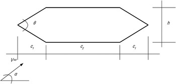
Here, a numerical method called the vortex-panel method is used in conjunction with the Kutta condition to obtain the unique solution Φ. A two-dimensional flow around a submerged body shown in Figure 1 is considered. The shape of the body resembles a typical cross-section of a low-drag aerodynamic box girder in bridges (Dowell et al., Reference Dowell, Peters, Clark, Scanlan, Cox, Simiu, Curtiss, Sisto, Edwards, Strganac and Hall2004). This shape ensures that the conditions of a potential flow are satisfied. The velocity of the fluid is denoted as V
∞, and the angle of attack as α. The surface of the body is divided into m number of vortex panels, forming a closed polygon. In Figure 1 the panels are indexed as i with the coordinates of two ends denoted as (X
i
, Y
i
) and (X
i+1, Y
i+1, and the outward normal vector denoted as
 ${\bf n}_i $
. The midpoint of panel i is referred to as the ith control point, and the corresponding coordinate is denoted as (X
i
, Y
i
). The circulation density γ(s
i
), where s
i
denotes the distance of a point on the ith panel from the vertex (X
i
, Y
i
), is assumed to vary linearly within each element. In addition, the interelement continuity of the circulation density is imposed except between elements 1 and m, which appear at the trailing edge. The circulation density at the vertex (X
i
, Y
i
) is denoted as γ
i
. The velocity potential at the ith control point (X
i
, Y
i
) can be expressed as (Kuethe & Chow, Reference Kuethe and Chow1986)
 $$\eqalign{\Phi (x_i\comma\, y_i ) = V_\infty (x_i \!\cos{\rm \alpha} + y_i \!\sin{\rm \alpha} ) -\sum \limits_{\,j = 1}^m \int\limits_{l_j} \displaystyle{{{\rm \gamma} (s_j )} \over {2{\rm \pi}}} & {{\rm tan}} ^{ - 1} \left( {\displaystyle{{y_i - y_j} \over {x_i - x_j}}} \right)ds_j\comma\ \quad \cr & i = 1\comma\,2\comma \ldots\comma \,m\comma\quad}$$
where l j denotes the length of the jth panel. In this expression, the integral over the length l j , combined with the summation over m elements, is an approximation of solution of Eq. (1). The boundary condition stated in Eq. (4) is imposed as
 $$\displaystyle{{\partial}\over {{\partial}n_i}} \Phi (x_i\comma \, y_i ) = 0\quad i = 1\comma \,2\comma \, \ldots\comma \, m\comma \,$$
where the ∂/(∂n
i
) operator denotes the directional derivative in the direction
 ${\bf n}_i $
. The boundary condition stated in Eq. (5) has already been taken into account by the V
∞ term in Eq. (6). Details of the procedures for performing the computations in Eqs. (6) and (7) are not presented here for brevity. However, these two sets of equations yield a system of m coupled linear equations with unknowns as
 $\left\{ {\rm \gamma} ^{\prime}_{i} \right\} _{i=1}^{m + 1}$
, where
 ${\rm \gamma} ^{\prime}_i $
denotes the value of γ
i
/2πV
∞. The first and the (m + 1)th node coincide, and they appear at the trailing edge. However, these two nodes need to retain their indices 1 and m + 1 for imposing an additional condition to ensure smooth flow at the trailing edge. This condition, termed as the Kutta condition, is expressed as
 $${\rm \gamma}^{\prime}_1 + {\rm \gamma}^{\prime}_{m + 1} = 0\comma \,$$
and is derived by equating the strength of the vorticity at the trailing edge to zero. Inclusion of Eq. (8) makes the system of linear equations as m + 1 equations with m + 1 unknowns, stated as
 $$\sum\limits_{\,j = 1}^{m + 1} {} A_{N_{ij}} {\rm \gamma} ^{\prime}_j = p_i \quad i = 1\comma \,2\comma \, \ldots\comma \,m + 1.$$
The scalar
 $A_{N_{ij}} $
s are referred to as the normal-velocity influence coefficients. This equation can be written in the matrix notations as
 $${\bf A \Gamma} = {\bf p}\comma \,$$
where A is an (m + 1) × (m + 1) matrix, referred to as the influence coefficient matrix, with the (i, j)th term as
 $A_{N_{ij}} $
, and Γ and p are (m + 1)-dimensional vectors with entries
 ${\rm \gamma} ^{\prime}_j $
and p
i
, respectively. Once the unknown circulation densities
 ${\rm \gamma}^{\prime}_j $
s are determined by solving Eq. (10), the total lift force L acting on the submerged body is calculated as
 $$L = {\rm \rho} V_\infty \mathop \sum \limits_{i = 1}^m \left( {\displaystyle{{\rm \gamma}^{\prime}_i + {\rm \gamma}^{\prime}_{i + 1}} \over 2} \right) l_i \comma $$
where ρ denotes the density of the fluid. The lift coefficient by C L is computed as
 $$C_{\rm L} = \displaystyle{{2L} \over {{\rm \rho} V_\infty ^2 c}}\comma \,$$
where c = 2c 1 + c 2 is the chord length of the body.
Representation of the vortex-panel method.

3. THE PROPOSED SEMI-INTRUSIVE METHOD AND GLOBAL SENSITIVITY ANALYSIS
3.1. Proposed SISP method for lift prediction
In a perturbation framework, an improvement in accuracy and computational speed can be achieved if the perturbation is applied on the influence coefficient matrix A and the vectors Γ and p in Eq. (10), three intermediate quantities in a panel method. Usually perturbation methods in nonlinear equation perform well in a low variability regime. Here, we use perturbation in the linear part of the method [Eq. (10)] with the hope to get good estimates even at high variability. Let
 $\{{\rm \xi}_i \} _{i = 1}^n $
denote a set of zero-mean independent random variables characterizing the uncertainty, also collectively denoted by the vector ξ. According to this proposed method, let the quantities A, Γ, and p be expressed in their first-order approximation as
 $$\eqalign{ {\bf A}({\bf \xi} ) &= {\bf A}_0 + \sum\limits_{i = 1}^n {{\bf A}_i} {\rm \xi} _i\comma \, \quad {\bf \Gamma} ({\bf \xi} ) = {\bf \Gamma} _0 + \sum\limits_{i = 1}^n {{\bf \Gamma} _i} {\rm \xi} _i\comma \, \cr \quad \quad {\bf p}({\bf \xi} ) &= {\bf p}_0 + \sum\limits_{i = 1}^n {{\bf p}_i} {\rm \xi} _i\comma \,} $$
where
 $\{ {\bf A}_i \} _{i = 0}^n $
,
 $\{ \Gamma _i \} _{i = 0}^n $
, and
 $\{ {\bf p}_i \} _{i = 0}^n $
are deterministic coefficients. For computational purpose
 ${\bf A}_0 $
and
 ${\bf p}_0 $
can be chosen as the values of the quantities A and p at their nominal or mean level, that is, corresponding to ξ = 0, and the coefficients
 $\{ {\bf A}_i \} _{i = 1}^n $
and
 $\{ {\bf p}_i \} _{i = 1}^n $
can be estimated using a finite-difference approximation. To estimate
 $\{ {\bf \Gamma} _i \} _{i = 0}^n $
, substitute Eq. (13) in Eq. (10), which results in
 $$\left( {{\bf A}_0 + \sum\limits_{i = 1}^n {{\bf A}_i {\rm \xi}_i}} \right)\left( {\Gamma_0 + \sum\limits_{i = 1}^n {\Gamma_i {\rm \xi}_i}} \right) = \left( {{\bf p}_0 + \sum\limits_{i = 1}^n {{\bf p}_i {\rm \xi}i_i}} \right).$$
Matching the constants and the coefficients of the
 $\{{\rm \xi}_i \} _{i = 1}^n $
in both sides of this equation yields
 $${\bf \Gamma} _0 = {\bf A}_0^{ - 1} {\bf p}_0 $$
and
 $${\bf \Gamma} _i = {\bf A}_0^{ - 1} \left[ {{\bf p}_i - {\bf A}_i \Gamma_0} \right]\comma \quad i = 1\comma \,2\comma \, \ldots\comma \,n.$$
Let the jth element in the vector Γ
i
be denoted as
 ${\rm \gamma}^{\prime}_{j\comma \,i} $
. Then from Eq. (11), the lift can be found as
 $$\eqalign{ L({\bf \xi} )& = \displaystyle{{{\rm \rho} ({\bf \xi} )V_\infty ({\bf \xi} )} \over 2} \sum\limits_{j = 1}^m \bigg[ \lpar {{\rm \gamma^{\prime}}_{\hskip-2pt j\comma \,0} + {\rm \gamma^{\prime}}_{\hskip-2pt j + 1\comma \,0}} \rpar \cr & \quad \left. + \sum\limits_{i = 1}^n {\lpar {{\rm \gamma^{\prime}}_{\hskip-2pt j\comma \,i} + {\rm \gamma^{\prime}}_{\hskip-2pt j + 1\comma \,i}} \rpar } {\rm \xi}_i \right] l_j ({\bf \xi} ).} $$
Evaluation of L(ξ) for a given realization of ξ involves only multiplication and addition of a few scalar quantities. Therefore, performing a statistical simulation of L(ξ) using this expression to estimate the statistical moments and PDF of the lift will not be expensive, especially compared to the cost of MCS on the panel code.
In an intrusive approach in SSFEM, a number of intermediate matrices and vectors are required to be accessed (Ghanem & Spanos, Reference Ghanem and Spanos2003), similar to the proposed method. For instance, in an elliptic problem or an eigenvalue problem, the stiffness and mass matrices are sought (Ghanem & Ghosh, Reference Ghanem and Ghosh2007; Ghosh et al., Reference Ghosh, Avery and Farhat2009). However, it requires a new solver as well. However, in the proposed perturbation method, no new solver is needed. Therefore, this method is called semi-intrusive here.
3.2. Global sensitivity analysis: Sobol indices
Sobol’ decomposition of the function L(ξ), which is used to measure the sensitivity of the parameters based on their relative contribution toward the variance, is expressed as
 $$\eqalign{L(\xi ) & = L_0 + {\sum\limits_{1 \le i \le n}} {L_i (\xi _i )} + \sum\limits_{1 \le i \lt j \le n} {L_{ij} (\xi _i\comma \, \xi _j )} + \cdots \cr & \quad + L_{12 \cdots n} (\xi _1\comma \, \ldots\comma \, \xi _n ).}$$
There are total of 2 n terms (referred to as Sobol’ functions) in this decomposition, and they are orthogonal to each other with respect to the underlying probability measure of the random vector ξ. Let D, D i , D ij , … , D 12···n denote the variance of the functions L(ξ), L i (ξ i ), L ij (ξ i , ξ j ), … , L 12···n (ξ1, … , ξ n ), respectively. Then it can be shown (Sobol’, Reference Sobol’2001) that the equality
 $$D = \sum_{1 \le i \le n} {D_i} + \sum_{1 \le i \lt j \le n} {D_{ij}} + \cdots + D_{12 \cdots n} $$
is always satisfied. The Sobol’ indices are defined as
 $$\eqalign{ S_i = \displaystyle{{D_i} \over D}\comma & \,S_{ij} = \displaystyle{{D_{ij}} \over D}\comma \, \cdots\comma \, S_{i_1... i_s} = \displaystyle{{D_{i_1... i_s}} \over D}\comma \, \cdots\comma \, \cr & \quad S_{12...n} = \displaystyle{{D_{12 \cdots n}} \over D}.}$$
Therefore, these indices quantify the relative contribution of each term in Eq. (18) toward the total variance D, except the term L
0. The total sensitivity of a random parameter ξ
i
, denoted here as
 $S_i^{\rm tot} $
is measured as the sum of the sensitivities in Eq. (20) that contain the index i. For instance, if n = 4, the total sensitivity of the parameter ξ1 is
 $$S_1^{{\rm tot}} = S_1 + S_{12} + S_{13} + S_{14} + S_{123} + S_{124} + S_{134} + S_{1234}. $$
Here,
 $S_i^{{\rm tot}} $
is regarded as the global sensitivity of the variable ξ
i
. Therefore, compared to the local sensitivity
 $S_i^{{\rm loc}} $
, the global sensitivity
 $S_i^{{\rm tot}} $
includes not only the effect of the random variable ξ
i
on its entire support but also the effect of the cross-terms.
Estimation of the Sobol’ indices requires evaluation of multidimensional integrals (Sobol’, Reference Sobol’2001; Arawde et al., Reference Arwade, Moradi and Louhghalam2010) and is usually carried out through MCS. Evaluation of each variance
 $D_{i_1 \cdots i_s} $
requires a complete Monte Carlo run. Because there are 2
n
such variances including D, the total computation becomes very expensive for large n. To alleviate this problem, a PCE-based estimation procedure has recently been developed (Crestaux, Reference Crestaux, Le Maître and Martinez2009; Blatman & Sudret, Reference Blatman and Sudret2010), and is described next.
3.2.1. Estimation of the Sobol’ indices using polynomial chaos expansion
Let E{·} denote the mathematical expectation operator. Then the truncated PCE of the square-integrable function L(ξ) is expressed as (Ghanem & Spanos, Reference Ghanem and Spanos2003)
 $$L({\bf \xi} ) = \sum\limits_{i = 0}^{\,p - 1} {} L_i^{{\rm PC}} {\rm \psi} _i ({\bf \xi} )\comma \,$$
where ψ
i
(ξ) are orthogonal polynomial bases and p depends on the order of expansion and the number of input random variables n. Once the coefficients
 $L_i^{{\rm PC}} $
are estimated, the mean and variance of L(ξ) can be estimated as
 $$E\{ L({\rm\bf \xi} )\} = L_0^{{\rm PC}}\comma $$
 $$D = {\rm var}(L({\rm \bf \xi} )) = E\{ (L({\rm \bf \xi} ) - L_0^{{\rm PC}} )^2 \} = \sum\limits_{i = 1}^{P - 1} {(L_i^{{\rm PC}} )^2 E\{ {\rm \psi} _i^2 \}}. $$
The Sobol’ decomposition in Eq. (18) can be approximated by the truncated PCE in Eq. (22) through a regrouping of the chaos terms. The approximation error becomes zero when L(ξ) is a polynomial with the highest degree being less than or equal to the order of chaos. The procedure to find the index sets corresponding to this regrouping can be found in Crestaux (Reference Crestaux, Le Maître and Martinez2009) and Blatman and Sudret (Reference Blatman and Sudret2010) It should be noted that PCE requires a very large number of terms when n or order of expansion or both are high, often referred to as the curse of dimensionality. Adaptive sparse versions of PCE are proposed in Todor and Schwab (Reference Todor and Schwab2007) and Blatman and Sudret (Reference Blatman and Sudret2010) to reduce this dimensionality.
4. NUMERICAL STUDY
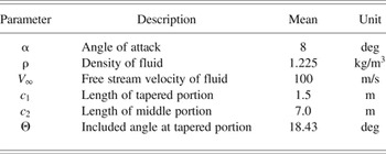
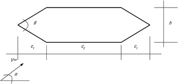
For numerical study an air flow around a body as shown in Figure 2 is considered here. The random parameters considered here are of two types: flow parameters, such as angle of attack (α), density of fluid (ρ), and free stream velocity (V ∞); and geometric parameters of the submerged body, such as lengths c 1 and c 2, included angle at the tapering ends (Θ). These six parameters are considered as six independent random variables, with their assumed mean values given in Table 1 leading to n = 6. Three different probability distributions are considered here: Gaussian, uniform, and log normal. For testing the SISP, all three distributions are considered, whereas for sensitivity analysis only the Gaussian distribution is considered. The numerical study is divided into two parts. In the first part, the SISP and tested, considering all the random variables. The estimates from the proposed method is compared with the estimates from MCS and perturbation directly on the lift. In the second part, a study is conducted to assess the relative performance of the local and global sensitivity indices. SISP is used to estimate the global sensitivity indices.
Submerged body with parameters involved.
Random parameters and their mean values

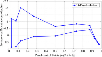
The surface of the submerged body is discretized using a number of vortex panels, as shown in Figure 2. The Matlab programming environment is used for all implementations including the panel method described in Section 2. A direct linear solver is used to solve Eq. (10). However, for large applications, an iterative solver might be more efficient. A numerical study is first conducted where the convergence of the lift force is observed with respect to the number of panels. From this study it is observed that 18 panels capture the lift force with sufficient accuracy, that is, m = 18. The coefficient of pressure on different panels estimated at the mean values of the parameters is shown in Figure 3. For practical applications, the number of panels may be as high as in the range of a few thousands (Hess, Reference Hess1990).
Pressure distribution on the panels.

4.1. Numerical study on lift prediction using the proposed method (SISP)
Implementation of the semi-intrusive method requires access to the influence coefficient matrix A and the vector p in Eq. (10). The matrices
 $\{ {\bf A}_i \} _{i = 0}^6 $
and vectors
 $\{ {\bf p}_i \} _{i = 0}^6 $
are then estimated using a finite difference approximation. After this approximation, the vector Γ
0 is computed by solving the linear system in Eq. (15). The other six Γ
i
s are then computed by substituting Γ
0,
 ${\bf A}_i $
, and
 ${\bf p}_i $
in the right-hand side of Eq. (16) and solving the resulting linear system for a given i. Finally, the statistical moments and PDF of the lift force is estimated by sampling from Eq. (17).
The perturbation analysis directly on the lift quantity (referred to here as direct perturbation) is performed where the panel code is used as a black box and the derivatives in this equation are approximated using a finite-difference scheme. Both first- and second-order expansions of the direct perturbation are used here. To study the relative performance of these perturbation methods, different combinations of variability levels in geometric and fluid parameters are considered. In a typical engineering application where the structure is designed and the flow is natural, the variability in the flow could be significantly higher than the variability in the structural or geometric parameters. Therefore, here the standard deviation in the geometric parameters of the body is kept fixed at 5% of their mean, whereas the standard deviation of the flow parameters is varied between 5% to 40% of their mean. In addition, a study is conducted for higher variability in the geometric parameters in Section 4.1.3. In all cases, the results are compared with the estimates from a MCS performed using 1 × 10⁴ realizations.
4.1.1. Case 1: Gaussian distribution
In the first set of numerical experiments, all the random variables are assumed to be independent Gaussian. That is, the variables
 $\{ {\rm \xi}_i \} _{i = 1}^6 $
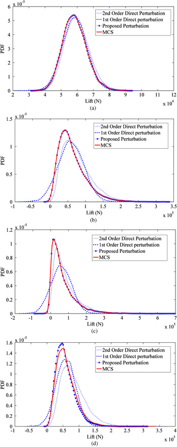
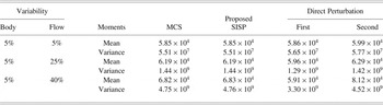
are independent standard normal. The estimated statistical moments are tabulated in Table 2, and the PDFs are plotted in Figure 4a–d. In Table 2, the first two columns represent the standard deviation of the geometric parameters of the body and of the flow parameters, respectively. For several combinations of these variabilities, the first two statistical moments (mean and standard deviation) of the lift estimated using MCS, proposed SISP, and direct perturbation are presented in the other columns. The following observations are made from this table: for low variability of the input parameters, that is, for 5% standard deviation of geometric and flow parameters, all the four methods yield similar estimates, with the SISP yielding a marginally better estimate; as the variability of flow parameters increases to 25%, the second-order direct perturbation yields better estimates than the first-order direct perturbation, but SISP performs significantly better; and as the variability of flow parameters becomes very high, that is, 40%, even the second-order direct perturbation results in significant error whereas as SISP yields remarkably close estimates to the estimates from MCS.
Comparison of probability density functions for various combinations of standard deviations of geometric and flow parameters with Gaussian distribution: (a) 5% standard deviation in both geometric and flow parameters, (b) 5% standard deviation in geometric and 25% standard deviation in flow parameters, (c) 5% standard deviation in geometric and 40% standard deviation in flow parameters, and (d) 20% standard deviation in geometric and 20% standard deviation in flow parameters.

Statistical moments of lift (N) estimated using different methods

Note: The input parameters follow Gaussian distribution.
The estimates of the PDFs are compared next. In Figure 4a–c, the variability in the flow parameters are increased progressively and the PDFs estimated using four methods are plotted. Here also it is noted that as the variability increases, the SISP yields a better estimate of the PDFs compared to the direct perturbation. However, when the variability is 25% or more, the first-order direct perturbation estimates are remarkably poor compared to the second-order direct perturbation. Note that in all these experiments, the SISP includes only first-order terms.
In terms of computational cost, the SISP is comparable to the direct perturbation method. Both of these methods require only a few (tens of) calls to the panel code, whereas the MCS requires a few thousand calls. The major cost in the panel code is to assemble the matrix A and solve Eq. (10), which usually varies between O(m 2) to O(m 3), depending upon the solver used. Therefore, as the number of panels m grows, the cost saving using the perturbation methods is significant compared to MCS. Therefore, for high variability in the input parameters, the SISP yields accurate estimates at a low computational cost.
4.1.2. Case 2: Non-Gaussian distributions: Log normal and uniform
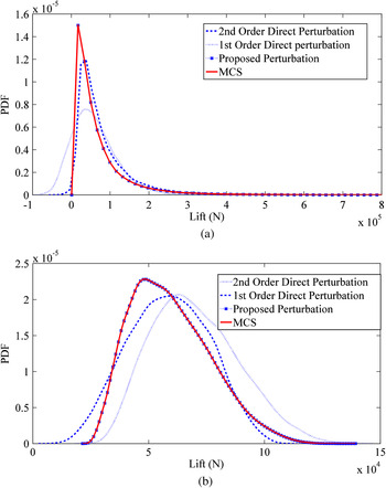
To test the robustness of SISP with respect to the probability distributions of the random parameters, two more distributions are considered in the next set of experiments: log normal and uniform. The aforementioned experiments performed for the Gaussian distribution are repeated for these two distributions and a representative set of results is given. PDFs of the lift corresponding to 5% variability of geometric parameters and 40% variability of flow parameters are plotted here. For log-normal distribution of the parameters the PDFs are plotted in Figure 5a, and for uniform distribution they are plotted in Figure 5b. It is observed that for both of these non-Gaussian distributions the SISP performs equally well as the Gaussian case.
Comparison of probability density functions with 5% standard deviation in geometric and 40% standard deviation in flow parameters: (a) log-normal distribution and (b) uniform distribution.

4.1.3. High variability in the geometric parameters
As mentioned earlier, a higher variability in the flow parameters is expected compared to the geometric parameters in a typical engineering setting. However, to test the accuracy of the proposed method, a case is considered where the geometric parameter also has high variability. In this case 20% standard deviation is assumed for both the geometric and flow parameters. The PDFs are plotted in Figure 4d. From this plot, it is observed that the accuracy of SISP estimates is lower compared to MCS when the variability of the geometric parameters is high. However, the accuracy is still better compared to the first- and second-order direct perturbation.
4.2. Application of the proposed SISP method in GSA
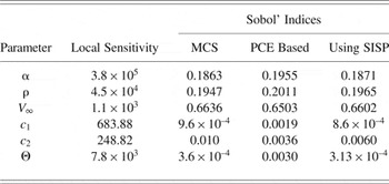
The proposed SISP method is next implemented for efficient estimation of global sensitivity, that is, Sobol’ indices. The sensitivity analysis of lift is carried out with respect to the six random parameters. Both LSA and GSA are carried out using the methods described in Section 3. For 5% variability in geometric parameters and 20% variability in the flow parameters the estimates of global sensitivities are reported in Table 3. The levels of variability in the input parameters are arbitrarily chosen for demonstration purpose only. The local sensitivities are estimated using a finite-difference approximation and reported in the second column of this table. The GSA is first carried out using both MCS and a second-order PCE on Eq. (11), and
 $S_i^{{\rm tot}} $
is reported as the sensitivity index in the third and fourth columns. Comparing the third and fourth columns of this table, it can be observed that PCE-based estimates match well with MCS estimates for a rank ordering purpose. Because the PCE approach is computationally cheaper than MCS, from this observation it can be concluded that for GSA the PCE approach is a better alternative of MCS. Next, a comparison of either of these two columns with the second column indicates that the local and global sensitivities give different rank ordering; however, Sobol’ indices obtained in the three cases have same rank ordering. Moreover, V
∞, the most important parameter according to GSA, does not appear in the list of three most important parameters according to LSA. Therefore, LSA estimates cannot be used for dimension reduction in a prediction problem where the entire supports of the random parameters are used.
Estimated sensitivity of lift force (L) with respect to the random parameters (Gaussian), for 5% variation in geometric parameters and 20% variation in flow parameters

To reduce the computational cost of GSA, the SISP coupled with a second-order PCE is next used. Accordingly, for each realization the lift is estimated using Eq. (17). The estimates thus obtained are reported in the fifth column of this table. From here also it is observed that the SISP yields excellent estimates of the sensitivity indices, with a lower computational cost.
5. CONCLUSIONS
The proposed SISP method is found to have an excellent accuracy in lift and global sensitivity prediction, even at a high level of variability of the parameters. It is computationally far less expensive compared to a direct simulation method, and the gain will be higher for larger problems. The accuracy is particularly higher when the variability in the geometric parameters is low. This computational speed-up will be useful in reliability-based design optimization. However, for low levels of variability, a direct perturbation of the lift yields good estimates, with comparable cost. One specific requirement for the proposed method is that it requires access to a matrix and a vector in the circulation density computation level of a panel method, similar to the intrusive approaches in spectral stochastic finite element methods. For in-house and open-source panel codes, this is easily achievable. However, for commercial solvers where such access is not straightforward this step will need further attention.
ACKNOWLEDGMENT
This work was carried out while the first author was a graduate student in the Indian Institute of Science, Bangalore.
Anup Suryawanshi is the Founder and Director of Subduction Zone Consultants, Pune.
Debraj Ghosh is an Associate Professor in the Department of Civil Engineering at the Indian Institute of Science.