Signal model

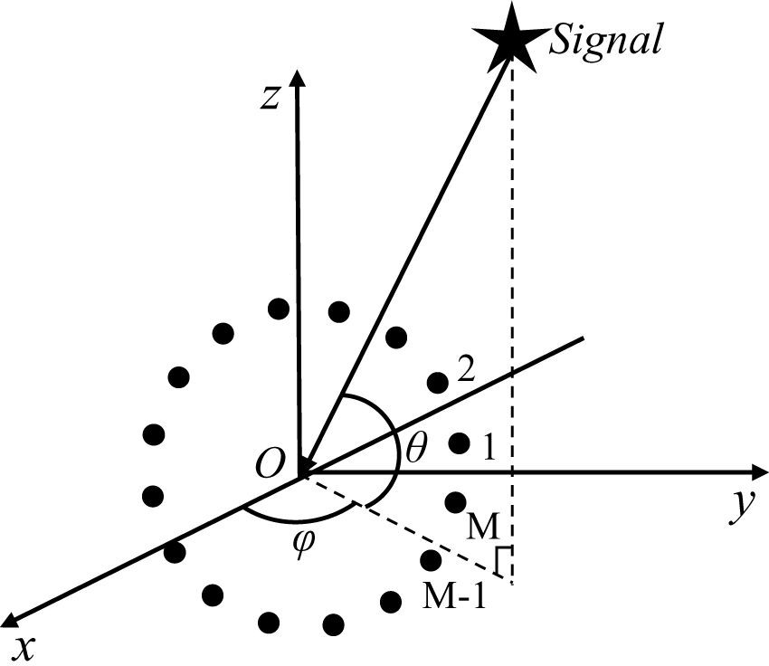
The UCA antenna consists of antenna elements that are uniformly distributed on a circle or multiple concentric circles. This paper mainly focuses on a single-ring UCA consisting of M = 16 elements. To enhance the beam coverage performance in three-dimensional space, the circular array has been arranged in the yoz plane, as shown in Figure 1.

Figure 1.

Uniform circular array model.

Consider a UCA with radius r, where M elements are uniformly distributed on the yoz plane. The center of the array circle coincides with the origin of the three-dimensional coordinate system, and the x-axis is the boresight direction. Under this coordinate configuration, the θ angle is measured from the x-axis. For the radiation scene that only covers the front half-space, the range of elevation angle θ and azimuth angle φ is θ ∈ [−90°, 90°] and φ ∈ [−90°, 90°], respectively. According to [Reference Haefner, Kaeske and Thomae22], when a plane wave with an incident direction of (θ, φ) reaches the array, the relative phase shift of the m-th array element relative to the center of the circle can be expressed as:

(1)\begin{equation}{\beta _m} = - kr(\cos {\theta _m}\cos \varphi \sin \theta + \sin {\theta _m}\sin \varphi )\end{equation}

where θ_m = 2π(m − 1)/M (m = 1, 2, …, M), k = 2π/λ, and r is the radius of the UCA. In the previous equation, θ_m denotes the polar angle coordinate of the m-th antenna element, k is the wave number, and λ is the wavelength of the signal.

α(θ, φ) denotes the steering vector of the signal with angle (θ, φ), and its general form is given by:

(2)\begin{equation} \boldsymbol{\alpha}(\theta,\varphi)=[e^{j\beta_1}, e^{j\beta_2}, \cdots, e^{j\beta_M},] \end{equation}

As described in [Reference Krim and Viberg23], in a UCA, assuming that the received signal consists of the desired signal, interference signals, and noise, the array received signal can be expressed as:

(3)\begin{equation} X(t)=\boldsymbol{\alpha}(\theta_s, \varphi_s)s(t)+\sum^1_{i=1}\boldsymbol{\alpha}(\theta_i, \varphi_i)s_i(t)+n(t)\end{equation}

where X(t) is the complex signal vector received by the array, α(θ_s, φ_s) and α(θ_i, φ_i) represent the steering vectors of the desired signal and the i-th interference signal, respectively. s(t) and s_i(t) represent the desired signal and the i-th interference signal, respectively, I is the number of interference sources, and n(t) is the additive noise, which is typically assumed to have a mean of 0 and follow a Gaussian white noise distribution.

The covariance matrix of the received signal is defined as follows:

(4)\begin{equation}R=E[X(t)X^H(t)]\end{equation}

In practical application, since the signal is of limited sampling, T samples can be used for estimation:

(5)\begin{equation}\mathop R\limits^ \wedge=\frac{1}{T}\sum^T_{t=1}X(t)X^H(t)\end{equation}

The goal of the MVDR beamforming algorithm is to minimize the output power while ensuring that the desired signal directional gain is not distorted, and thus, W_MVDR can be expressed as [Reference Capon24]:

(6)\begin{equation}{{\boldsymbol{W}}_{MVDR}} = \frac{{{{\mathop R\limits^ \wedge }^{ - 1}}\alpha ({\theta _{s,}}{\varphi _s})}}{{{\alpha ^H}({\theta _{s,}}{\varphi _s}){{\mathop R\limits^ \wedge }^{ - 1}}\alpha ({\theta _{s,}}{\varphi _s})}}\end{equation}

Construction and processing of datasets

The dataset used for neural network training in this paper has been generated through the simulation of a UCA. The training dataset has been generated based on the parameter settings in Table 1. The received covariance matrix and the corresponding weight vector obtained from each experiment are employed as the input data and the corresponding label W_label, respectively. Meanwhile, in order to enhance the robustness of W_label, the power ratio (INR) of the interfering signal to the desired signal is randomly varied within the range of 20–35 dB to simulate the diversity of interference strength in practical scenarios.

Table 1.

Parameter settings

After the input data and labels have been obtained, a preprocessing operation is required before feeding the data into the neural network for training in order to enhance the adaptability of the model to the input data. First, it is necessary to process the input features using the max-min normalization principle [Reference Zhu, Qi and Feng25], which can be expressed as:

(7)\begin{equation}\mathop R\limits^ \wedge = \frac{{\mathop R\limits^ \wedge - {{\mathop R\limits^ \wedge }_{\min }}}}{{{{\mathop R\limits^ \wedge }_{\max }} - {{\mathop R\limits^ \wedge }_{\min }}}}\end{equation}

where ${\mathop R\limits^ \wedge _{\max }}$ and ${\mathop R\limits^ \wedge _{\min }}$ represent the maximum and minimum values of the covariance matrix, respectively. Since the obtained $\mathop R\limits^ \wedge $ is a complex matrix, considering the real-number processing characteristics of deep learning frameworks, the normalized real and imaginary parts of $\mathop R\limits^ \wedge $ are separated and concatenated into a two-channel structure X as input to the neural network:

(8)\begin{equation}\,X = \left[ {{{\mathop R\limits^ \wedge }_{real,}}{{\mathop R\limits^ \wedge }_{imag}}} \right]\end{equation}

Specifically, this can be written as:

(9)\begin{equation}X(i,j,k) = \left\{ {\begin{array}{*{20}{c}} {\operatorname{Re} (\mathop R\limits^ \wedge (i,j))}&{k = 1} \\ {\operatorname{Im} (\mathop R\limits^ \wedge (i,j))}&{k = 2} \end{array}} \right.{\text{ }}\end{equation}

In the above equation, i and j denote the indices of the rows and columns of the matrix, respectively, and k takes different values to represent the real and imaginary channels, respectively.

Similarly, due to the significant variation in the data magnitudes of the labels, some smaller magnitudes still contain a lot of feature information, which can be easily overlooked by the neural network. To solve this problem, experimental results have verified that processing the label by magnifying it 100 times is more effective. For the amplified W_label, it is converted into a real-valued vector by decoupling its real and imaginary components:

(10)\begin{align} {W_{label}} =& \left[ \right.\operatorname{Re} \left\{ W_1\right\},\operatorname{Re} \left\{ W_2 \right\}, K \operatorname{Re} \left\{ W_M \right\},\operatorname{Im} \left\{ W_1 \right\}, \cr & \operatorname{Im} \left\{ {{W_2}} \right\}, K \operatorname{Im} \left\{ {{W_M}} \right\}\left. \right]^T \end{align}

To enhance the model’s generalization, the training set includes multiple combinations of angles and INRs, and a total of N sets of samples are generated, and the final dataset is denoted as:

(11)\begin{equation}{T_{train}} = \bigcup\limits_{n = 1}^N {\left\{ {({X_N},{W_{label,n}})} \right\}} \end{equation}

80% of T _train is divided into a training set for the model’s learning process and 20% is divided into a validation set for evaluating the performance of the model on unseen data. Finally, the T _train dataset is trained using the neural network mentioned in this paper to handle the beamforming task with deep learning algorithms.

Anti-interference performance evaluation metrics

One of the metrics for evaluating the model’s anti-interference performance is the null depth at the interference signal angle, which reflects the model’s ability to suppress interference signals. Generally, the deeper the null depth, the better the model’s anti-interference performance. The other metric is the output SINR, which can directly reflect the energy ratio of the target signal to interference and noise. In practical applications, an output SINR of more than 20 dB ensures high communication quality.

Structure of IRDSNet

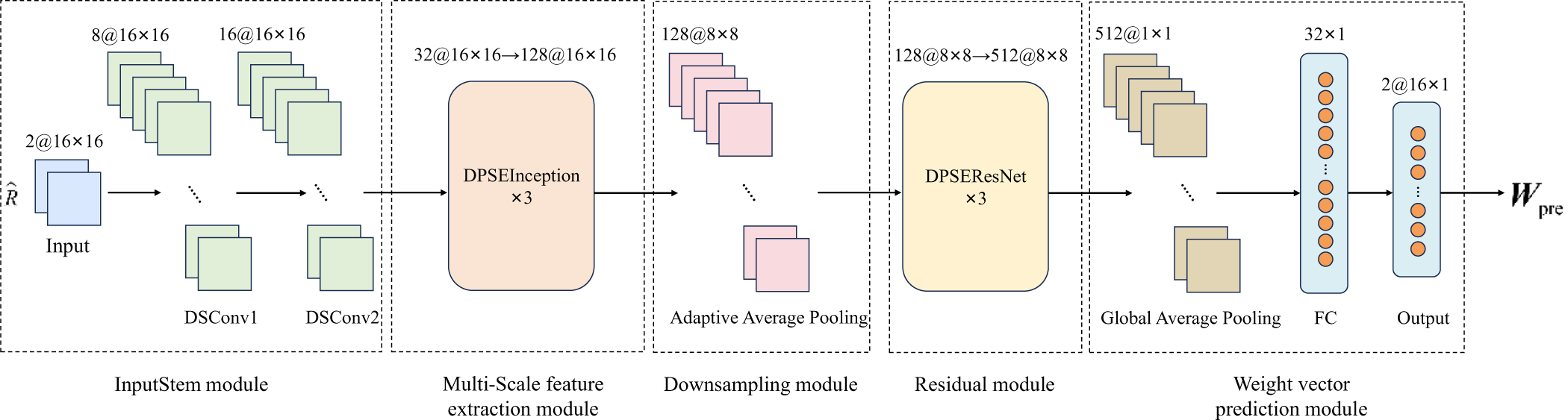
The proposed IRDSNet model is displayed in Figure 2. This module consists of the InputStem module, an improved channel attention mechanism module, a multi-scale feature extraction module, a downsampling module, a residual module, and a weight vector prediction module. The following sections provide a detailed description of each module.

Figure 2.

Proposed IRDSNet module.

InputStem module

The IRDSNet algorithm uses the covariance matrix of the received signal as the original input data, which is a 16 × 16 complex matrix, where 16 represents the number of elements in the UCA. The input data to the neural network has a shape of 2 × 16 × 16. After receiving the input, the network processes it through two DSConv layers with a kernel size of 3 × 3. Padding and stride are both set to 1, expanding the number of channels from 2 to 16. At the same time, low-level features are extracted to provide input data for the subsequent multi-scale feature extraction module.

Improved channel attention mechanism module

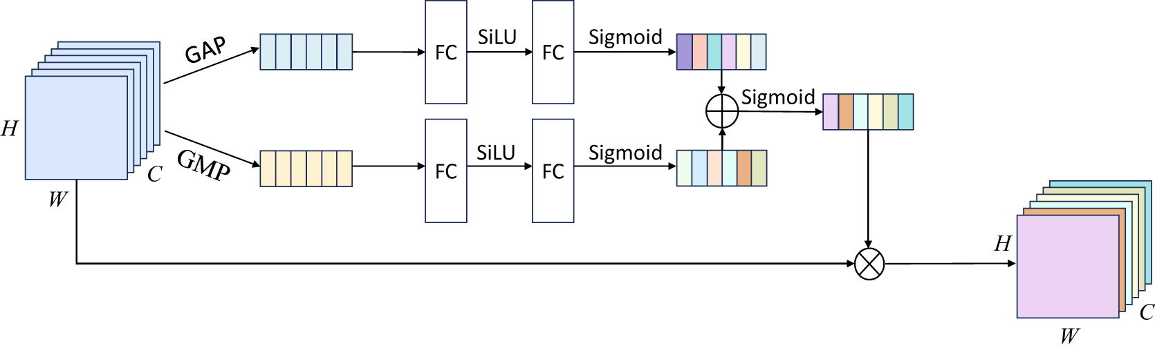
This paper proposes a channel attention mechanism based on SENet improved dual-pool feature fusion (dual-pool Squeeze-and-Excitation Network, DP-SENet) as shown in Figure 3. Compared to SENet, DP-SENet innovatively introduces a parallel dual-pooling structure combining Global Average Pooling (GAP) and Global Max Pooling (GMP), where GAP tends to extract the global distribution information while GMP focuses on the local information in the feature map. This design enables complementary channel feature extraction, and it is expressed as:

(12)\begin{equation}{z_{avg}} = {F_{GAP}}(X) = \frac{1}{{H \times W}}\sum\limits_{i = 1}^H {\sum\limits_{j = 1}^W {{X_{c,i,j}}} } \end{equation}

(13)\begin{equation}{z_{\max }} = {F_{GMP}}(X) = \mathop {\max }\limits_{i,j} ({X_{c,i,j}})\end{equation}

Figure 3.

DP-SENet module.

Here, c is the channel index, i and j represent the position indices of the feature map, X is the input feature map, and z _avg and z _max represent the average activation value and the maximum activation value of each channel, respectively. Meanwhile, the module adopts the Sigmoid Linear Unit (SiLU) activation function to replace the Rectified Linear Unit (ReLUs) activation function in the original module; the smoothness and nonlinear characteristics of SiLU are better than ReLU, which enables the model to better capture the complex feature relationships. Finally, the robustness of the channel weight computation is improved by adding the outputs of the two branches. Specifically, the SiLU activation function can be expressed as [Reference Hwang and J26]:

(14)\begin{equation}SiLU = x \cdot \sigma (x)\end{equation}

In the above equation, σ(x) represents the Sigmoid function. The SiLU activation function has a continuous and differentiable curve near x = 0, which helps avoid the gradient vanishing problem that may occur with ReLU, while still maintaining the capability of nonlinear mapping. Based on this, the channel weight calculation process of DP-SENet can be expressed as follows:

(15)\begin{equation}s = \sigma ({W_2} \cdot SiLU({W_1} \cdot {z_{avg}})) + \sigma ({W_2} \cdot SiLU({W_1} \cdot {z_{\max }}))\end{equation}

W ₁ and W ₂ are the weights of the fully connected layers for dimensionality expansion and reduction, respectively, and r is the dimensionality reduction ratio. Ultimately, the selective enhancement of important channels is achieved by applying the computed channel weights s to the original feature map. In this way, DP-SENet is able to quantify the importance of the feature channels more accurately by fusing the dual-channel information, which significantly improves the feature extraction capability of the model.

Multi-scale feature extraction module

Traditional CNNs typically use convolutional kernels of a single size, which limits their ability to extract features at different scales. Therefore, inspired by the multi-branch architecture of Inception, this approach combines convolutional kernels of different sizes in parallel. This allows the model to extract multi-scale information and integrate features from different receptive fields, thereby enhancing the model’s feature extraction capabilities. To enable the model to significantly reduce computational complexity while maintaining feature expressiveness, DSConv and Ghost Conv are introduced to replace traditional convolution in the Inception architecture. DSConv significantly reduces the computational load of models by decomposing traditional convolution operations into depthwise convolution and pointwise convolution. Ghost Conv achieves feature channel expansion at a lower computational cost by generating redundant feature maps through linear transformations.

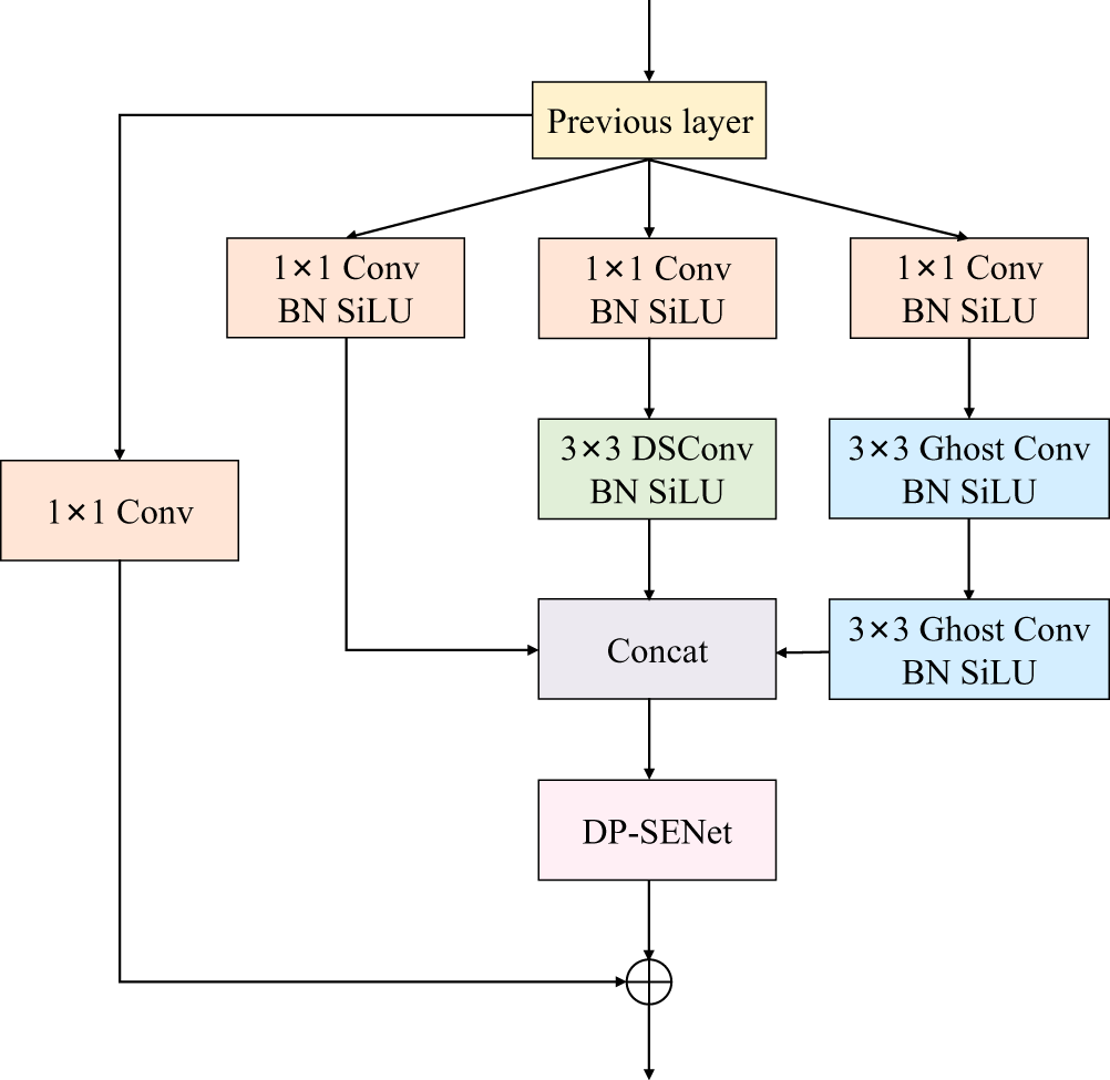
The module consists of a number of identically structured DPSEInception units, where each unit contains three branches, as shown in Figure 4. The first branch extracts global features rapidly using a 1 × 1 convolutional kernel. The second branch first reduces the number of channels of the feature map by a 1 × 1 convolutional kernel, followed by a 3 × 3 convolutional kernel, a layer of convolution with a larger receptive field for capturing local structural information of the input data. In the third branch, a 1 × 1 convolution is followed by the stacking of two 3 × 3 convolutions. The two 3 × 3 convolutions can be equated to a convolution of size 5 × 5, which can extract deeper local features while expanding the receptive field. In the DPSEInception unit, the 3 × 3 convolution in the second branch is replaced with a DSConv. This modification reduces the computational cost of large-kernel operations while maintaining channel-wise spatial processing capabilities. In the third branch, replacing the two 3 × 3 convolutions with Ghost Conv maintains feature diversity while significantly reducing parameter count, thereby addressing the limitation of DSConv in deep channel interactions. After splicing the outputs of the three branches, they are dynamically weighted by an improved channel attention mechanism, which enhances the expressive power of the model. Finally, the fused features and input features are summed by residual concatenation to output a higher-dimensional feature map.

Figure 4.

DPSEInception unit.

Downsampling module

The IRDSNet algorithm uses adaptive average pooling as the downsampling module, which is able to achieve efficient conversion from input to fixed-size output while retaining as much original information as possible by dynamically adjusting the pooling kernel size and stride parameters. In this paper, the 16 × 16 covariance matrix output from the multi-scale feature extraction module is adaptively downsampled to an 8 × 8 size by the downsampling module, which effectively reduces the number of parameters in the subsequent computation process and significantly improves the model’s computational efficiency.

Residual module

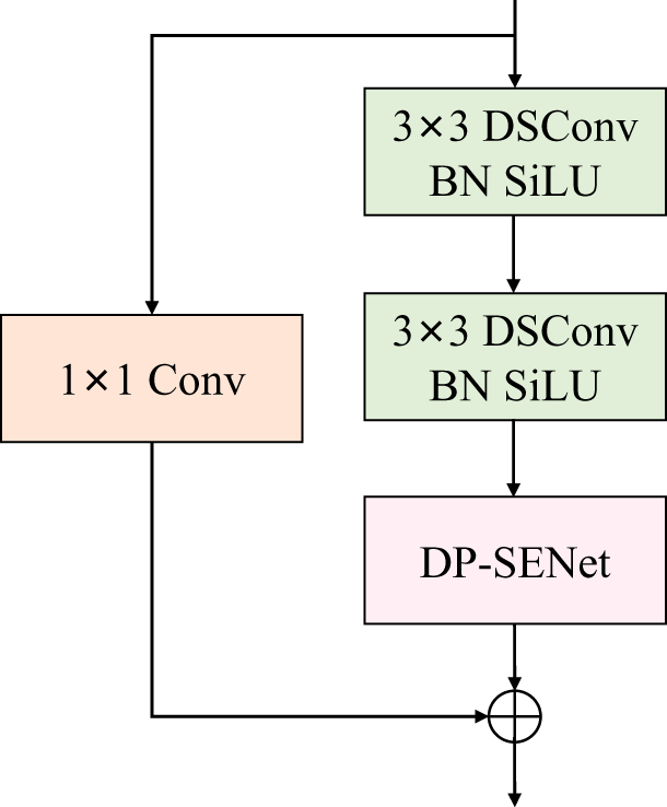
To make the weight vector output from the model closer to the optimal weight vector, IRDSNet uses the residual module to extract deep features. This module consists of multiple structurally identical DPSEResNet units, as shown in Figure 5. Each unit extracts features through two layers of DSConv with the same structure, where the kernel size of each DSConv is 3 × 3, with padding and stride both set to 1. After each convolution layer, batch normalization and the SiLU activation function are sequentially applied. Based on this structure, an improved channel attention mechanism is incorporated into the residual unit to focus the model on more important features. When the input and output channels do not match, the number of input channels is adjusted using 1 × 1 convolution to ensure that the input data can be residually summed with the output data of the main branch.

Figure 5.

DPSEResNet unit.

Weight vector prediction module

In the output stage of IRDSNet, the network uses a GAP module to replace the flatten layer operation. This approach significantly reduces computational complexity while preserving global channel information. Then, a fully connected layer is used to compress high-dimensional features, reducing feature redundancy while extracting core feature information. Finally, the output is reshaped into a 2 × 16 tensor, where the first dimension 2 represents the dual channel, which corresponds to the real and imaginary parts of the predicted weight vector, each containing 16 values. This transforms the task of predicting the weights of beamforming into a neural network regression problem, enabling the model to directly output parameters related to the directionality of the beam, thereby greatly improving the performance of wireless communication systems.

Determining the optimal model architecture

Multiple experiments were initially conducted to determine the optimal depth of the model, and preliminary experiments revealed that the DPSEInception and DPSEResNet units exhibit strong functional complementarity, with the former focusing on multi-scale feature extraction and the latter optimizing residual learning for retaining detailed information. Experiments have confirmed that these two modules, when used in combination, provide a significant improvement in performance over adding either module alone. To determine the optimal structure of IRDSNet, a series of experiments were designed, as shown in Table 2. Considering the balance between network complexity and training stability, these experiments progressively increased the number of DPSEInception and DPSEResNet units from the simplest model to evaluate the impact of network depth on beamforming performance. After determining the optimal network depth, experiments were conducted by removing the DP-SENet module and replacing the DSConv and GhostConv modules with standard convolution. The average null depth, Smooth L1 Loss, and parameter count were used as the evaluation metrics. The average null depth was calculated from the results of 20 groups of different interference angles, so as to comprehensively evaluate the role of each key module.

Table 2.

Comparison of different architectures

As shown in Table 2, when DPSEInception and DPSEResNet are used in combination and stacked in one or two layers, the number of parameters of the model is relatively small at this point, and the training speed is faster. However, the defect is that the average null depth is insufficient, and the corresponding Smooth L1 Loss is relatively high, which suggests that there is a bottleneck in the performance of the shallow network in the task of interfering signal suppression and regression. When the number of modules is increased to four layers, the number of parameters increases dramatically and the training time is also lengthened, but the average null depth improves less compared to when the number of modules is stacked in three layers. Therefore, we have chosen to stack two modules simultaneously three times as the structure of our proposed IRDSNet.

After determining the optimal depth of the model, the next step is to optimize the design of the number of channels internal to the module. The three DPSEInception units in the multi-scale feature extraction module are used to form a three-layer hierarchical structure by adopting a progressive channel expansion strategy, gradually increasing from 16 to 128. The shallow structure with fewer channels reduces computational overhead and captures low-level features, while subsequent layers with extended channels enable the model to learn more complex high-level semantic representations. Similarly, the number of channels in each DPSEResNet unit in the residual module also takes a gradually increasing approach, with the number of channels increasing from 128 to 512, allowing the model to expand the feature space in the shallower layers of the network to capture richer detail information, while the number of channels in the deeper layers is used to maintain a high feature representation and ensure the ability to learn complex patterns.

Further experiments demonstrate that the attention mechanism and lightweight convolutional modules are crucial to the model. After removing the attention mechanism module, the model’s parameters decreased slightly, but the average null depth was 12 dB different from the optimal model. This indicates that adding the attention mechanism to the model enables the model to pay more attention to the important features, and strengthen the expression ability of the model to interference-related feature channels. When the model replaces the lightweight convolution module with the standard convolution, the model’s parameters greatly increase and the training time becomes significantly longer. This surge in parameters and training time makes the model face higher computational resource requirements and longer response latency in real deployment, and the average null depth has limited improvement compared to the optimal model, which is not enough to offset the impact of the increase in parameters and training time. This demonstrates that the application of lightweight convolution module in the model is efficient and necessary, which can make the model achieve a good balance between interference suppression performance and computational efficiency.

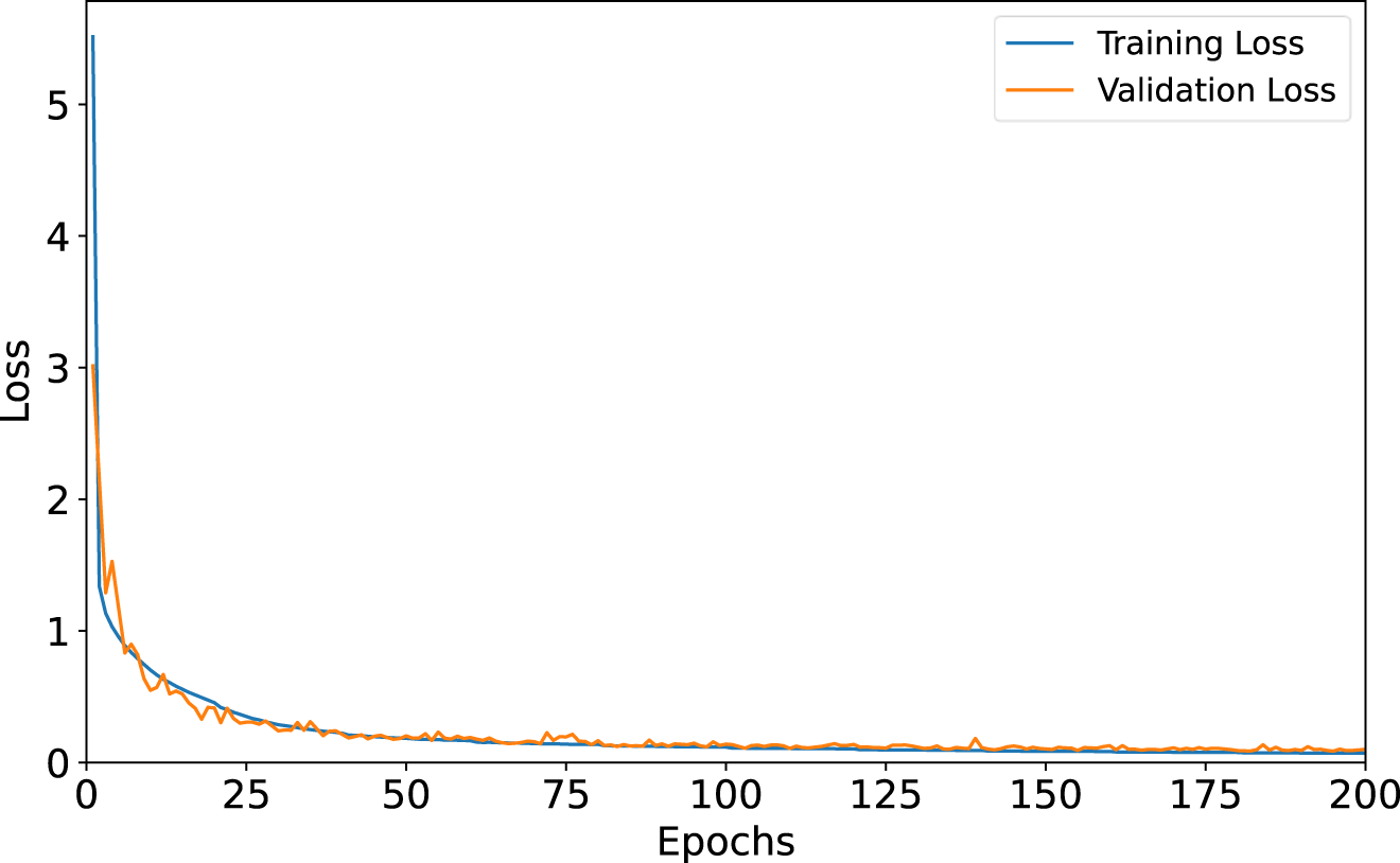
Figure 6 shows the loss function curves of the training and validation sets under the optimal model, and it can be seen that the loss curve decreases rapidly in the early stage of training and then gradually converges. This is mainly due to the preprocessing operations performed on the data before feeding it into the neural network for training, as well as the use of the Smooth L1 loss function, which allows the model to achieve fast and stable convergence. The strong consistency between the training loss and validation loss curves indicates that the model is neither overfitting nor underfitting. Instead, it has effectively learned the essential features of the data, achieving an ideal state of convergence.

Figure 6.

Training and validation loss curves.

Model fitting capability analysis

To evaluate the performance of the IRDSNet algorithm proposed in this paper, a comparison experiment with other existing algorithms is performed next. In the experiment, the received signal model contains the desired signal from the (θ = 0°, φ = 0°) direction and a single interference signal. In order to compare the effect under different interference angles, the single interference signal scenarios from (θ = 20°, φ = 40°) and (θ = −20°, φ = −35°) in two different directions were selected for the experiments, respectively. The INR is 30 dB in both scenarios and the noise is additive Gaussian white noise. The IRDSNet algorithm proposed in this paper is compared with the Eigen-Projection Processing (EMP) method [Reference Mao, Li and Luo28], WBPNet method [Reference Wu, Luo, Li, Zhang and Sheng17], MACNN method [Reference Liu, Yang, Yu, Du and Zhang20], and PRCNN method [Reference Sallam and Attiya16].

Figure 7 shows a comparison of the amplitude and phase of the output weight vectors of the deep learning-based beamforming algorithm at two different interference angles. From the figure, it can be seen that the IRDSNet algorithm fits the labels well in terms of amplitude and phase at each array element. By observing the enlarged subplots, it can be observed that the fitting effect of the IRDSNet algorithm is much better than the other compared algorithms. It shows that the proposed algorithm has better feature extraction capabilities and can analyze the input signal in more detail. Table 3 presents a comparison of Mean Absolute Error (MAE) between different algorithms, and the proposed algorithm has the lowest MAE as compared to other algorithms. It is shown that the proposed algorithm has a better fitting ability to make the model output beam pattern closer to the label-generated beam pattern, as well as a better output SINR performance.

Figure 7.

Comparison of amplitude and phase at different interference angles: (a) the amplitude at θ = 20°, φ = 40°; (b) the phase at θ = 20°, φ = 40°; (c) the amplitude at θ = −20°, φ = −35°; and (d) the phase at θ = −20°, φ = −35°.

Table 3.

Comparison of mean absolute error between different algorithms

Beampattern performance analysis

Figure 8 shows both directional diagrams and top views for two different interference angles, effectively demonstrating the interference signal angles and their corresponding null depths. However, due to the large number of angles involved in the 3D antenna orientation map, it is difficult to locate the interference source precisely. Therefore, to more accurately assess the beamforming effect, the cross-sectional diagrams at different interference angles are chosen to compare the beamforming algorithms.

Figure 8.

Uniform circular array antenna radiation pattern: (a) antenna radiation pattern at θ = 20°, φ = 40°; (b) antenna top view at θ = 20°, φ = 40°; (c) antenna radiation pattern at θ = −20°, φ = −35°; and (d) antenna top view at θ = −20°, φ = −35°.

The experiment selected the azimuth direction diagram cross-section at an elevation angle θ = 20° and the elevation direction diagram cross-section at an azimuth angle φ = 40°, as well as the azimuth direction diagram cross-section at an elevation angle θ = −20° and the elevation direction diagram cross-section at an azimuth angle φ = −35° for comparative verification, as shown in Figure 9. From the figure, it can be seen that compared to other algorithms, the IRDSNet algorithm proposed in this paper shows significant advantages in that its output direction diagram accurately fits the output of the original labels, and is able to form a deep null under the interference positions corresponding to the arrows. Compared to existing algorithms, although the EMP traditional algorithm can effectively block the mainlobe interference, it has strict requirements for the estimation of the angle of the interference signal, and its performance is poor in complex environments, so the algorithm has a poor fitting effect. The WBPNet algorithm has only a 3-layer shallow network structure, with a limited receptive field range and insufficient nonlinear expression capabilities, making it difficult to effectively extract more complex features. Although the MACNN algorithm introduces an attention mechanism, the simple stacking of two convolutional layers and an attention mechanism makes it impossible for the model to establish deep correlations between cross-channel features, resulting in insufficient null depth under interference angles, which cannot satisfy practical application requirements. The PRCNN algorithm introduces a max pooling downsampling operation, which improves computational efficiency but loses a lot of high-frequency feature information.

Figure 9.

Comparison of cross-sectional diagrams when interference signals are incident: (a) θ = 20°; (b) φ = 40°; (c) θ = −20°; and (d) φ = −35°.

Comparison of output SINR

Table 4 shows the comparison of the output SINR of several beamforming algorithms at different interference angles, and four different interference angles can simulate different scenarios. It can be seen that the proposed algorithm exhibits the best output SINR performance, with output SINR higher than 23 dB in different scenarios, which is comparable to or even slightly better than the MVDR algorithm. Meanwhile, the performance of IRDSNet is higher than that of other compared algorithms in all four interference scenarios, indicating that the proposed algorithm has strong feature extraction capabilities and excellent generalization ability. This allows the model to adapt to the beamforming task in different interference environments, thus ensuring communication quality and further validating its efficiency in beamforming tasks.

Table 4.

Comparison of output SINR at different interference angles (dB)

Comparison of inference time

Table 5 shows the comparison of inference time between different algorithms, each using the batch processing time of 100 covariance matrices as the benchmark for inference time. The initial calculation bias is eliminated by GPU warm-up before inference, while the average time of 10 inference times is taken as the final result in order to minimize the impact of inference errors. Since the EMP algorithm is a traditional anti-interference algorithm that requires a lot of matrix operations, it has no advantage in terms of inference time. The WBPNet and PRCNN algorithms are simple in structure and can be implemented with only a few simple convolutional layers, resulting in short inference times. However, they perform poorly in terms of interference suppression and output SINR. The inference time of the proposed algorithm is slightly longer than that of the MACNN algorithm, but the null depth of IRDSNet is about 30 dB deeper than that of the MACNN at the interference angle, while having a higher output SINR than that of the MACNN algorithm. Moreover, by incorporating DSConv and Ghost Conv into the model, the inference time has been effectively controlled within an acceptable range. This inference speed is efficient enough in scenarios such as dynamic wireless communications and radar systems to fully satisfy the real-time requirements of practical applications.

Table 5.

Comparison of inference time between different algorithms (sec)