1. Introduction
The superposition of a sinusoidal pulsation on a steady shear flow results in an oscillating response of the flow quantities. This type of flow arises in a wide range of engineering applications, including the flow in hydraulic turbines, turbomachines and combustion engines. Because of its practical importance, this type of flow has been the topic of many analytical, numerical and experimental studies. Previous studies have primarily focused on the near-wall behaviour of the time-averaged and oscillating components of the wall shear stress, velocity field and turbulence field. Analytical solutions to pulsed laminar flows in pipes and channels, termed Stokes laminar solutions because of their similarity to Stokes’ second problem of the flow resulting from an oscillating plate, can be found in Uchida (Reference Uchida1956) and Telionis (Reference Telionis1981), respectively. However, in the turbulent regime, investigations have been restricted to experimental and numerical studies, even though closed-form expressions for the amplitude of the oscillating wall shear stress have been derived for low-frequency pulsations (Mao & Hanratty Reference Mao and Hanratty1986; Tardu, Binder & Blackwelder Reference Tardu, Binder and Blackwelder1994; Ismael & Cotton Reference Ismael and Cotton1996).
In previous studies (Tardu et al.
Reference Tardu, Binder and Blackwelder1994; Scotti & Piomelli Reference Scotti and Piomelli2001; He & Jackson Reference He and Jackson2009), successful correlations of the near-wall response of the oscillating flow quantities have been obtained with the Stokes length scaled in viscous units
 $l_{s}^{+}=l_{s}\bar{u}_{{\it\tau}}/{\it\nu}$
, where
 $l_{s}=\sqrt{2{\it\nu}/{\it\omega}}$
,
 ${\it\nu}$
,
 ${\it\omega}$
and
 $\bar{u}_{{\it\tau}}$
are the laminar Stokes length, the kinematic viscosity, the angular forcing frequency and the time-averaged friction velocity, respectively. The Stokes length is a measure of how far the oscillating shear layer generated at the wall diffuses into the flow. This length scale is derived from the laminar solutions and Stokes’ second problem. A similarity parameter equivalent to the Stokes length,
 ${\it\omega}^{+}={\it\omega}{\it\nu}/\bar{u}_{{\it\tau}}^{2}=2/l_{s}^{+^{2}}$
, which is the angular forcing frequency scaled in wall units, has frequently been used in place of
 $l_{s}^{+}$
(Mao & Hanratty Reference Mao and Hanratty1986; Finnicum & Hanratty Reference Finnicum and Hanratty1988). Based on
 $l_{s}^{+}$
(or
 ${\it\omega}^{+}$
), the oscillating flow has been classified into different regimes, each with different characteristics. These regimes are briefly discussed below, but the reader is referred to He & Jackson (Reference He and Jackson2009) or Manna, Vacca & Verzicco (Reference Manna, Vacca and Verzicco2012) for a more thorough discussion. The absolute values of
 $l_{s}^{+}$
, which have been used to distinguish the regimes, differ to some extent in the literature and are difficult to determine precisely.
When
 $l_{s}^{+}$
is of
 $O(1)$
, the flow is in the high-frequency regime. The oscillating shear layer generated at the wall is thin and confined within the viscous wall region. Outside the viscous sublayer, the oscillating shear is zero and the oscillating velocity is advected back and forth, similar to a plug. The modulation of turbulence is zero, implying a distribution of turbulence identical to that of a steady flow at the average Reynolds number. The inner and outer layers of the flow are completely uncoupled. When the frequency is lowered and
 $l_{s}^{+}$
is of
 $O(5{-}10)$
, the flow is in the quasi-laminar regime. A substantial portion of the flow remains unaffected by the imposed unsteadiness. However, the inner and outer regions start to interact because the oscillating shear generated at the wall propagates beyond the viscous sublayer. The oscillating wall shear stress and velocity field tend towards the laminar Stokes solution, thereby justifying the regime’s name: quasi-laminar. In the intermediate-frequency regime,
 $10<l_{s}^{+}<20$
, a stronger coupling between the inner and outer layers occurs. The shear layer is significant over a substantial portion of the radius, but a region still exists around the centre of the pipe with zero modulation of turbulence and a uniform oscillation of the velocity. A notable feature of the oscillating wall shear stress in this regime is that the amplitude is smaller than the laminar value for a range of
 $l_{s}^{+}$
, which implies that the turbulence decreases the oscillating shear in this regime. As
 $l_{s}^{+}$
is gradually increased, the oscillating flow transitions into the low-frequency regime and eventually the quasi-steady regime. The extent of the frozen region diminishes, and, for sufficiently large
 $l_{s}^{+}$
, the entire flow will be affected by the oscillations. In the quasi-steady regime, the flow does not differ from a steady flow at the same instantaneous Reynolds number. As argued by Binder, Tardu & Vezin (Reference Binder, Tardu and Vezin1995), at values of
 $l_{s}^{+}$
above
 ${\sim}$
12, the oscillating shear layer is larger than
 $l_{s}^{+}$
because the shear generated at the wall propagates beyond the viscous sublayer, in which the oscillations interact with the steady turbulence field. This interaction is not captured by the laminar Stokes length; therefore, Scotti & Piomelli (Reference Scotti and Piomelli2001) extended the concept of this parameter by introducing a turbulent Stokes length,
 $l_{t}$
. They defined an effective viscosity as the sum of the molecular and eddy viscosities such that
 $l_{t}=\sqrt{2({\it\nu}+{\it\nu}_{t})/{\it\omega}}$
. By taking the eddy viscosity as
 ${\it\nu}_{t}={\it\kappa}\bar{u}_{{\it\tau}}l_{t}$
, where
 ${\it\kappa}$
is the von Kármán constant, it follows that
 $$\begin{eqnarray}l_{t}^{+}=l_{t}\bar{u}_{{\it\tau}}/{\it\nu}=l_{s}^{+}\left[({\it\kappa}l_{s}^{+}/2)+\sqrt{1+({\it\kappa}l_{s}^{+}/2)^{2}}\right].\end{eqnarray}$$
It was shown that
 $l_{t}^{+}$
measures both the distance and at which speed that the shear wave generated at the wall travels into the core flow. Despite the assumptions involved when defining
 ${\it\nu}_{t}$
, the turbulent Stokes length was shown to correlate the data of Scotti & Piomelli (Reference Scotti and Piomelli2001) rather well.
Laser Doppler velocimetry (LDV) measurements of turbulent pulsating flows with different geometries have been performed by many research groups. For example, Tu & Ramaprian (Reference Tu and Ramaprian1983), Lodahl, Sumer & Fredsoe (Reference Lodahl, Sumer and Fredsoe1998) and He & Jackson (Reference He and Jackson2009) performed measurements in pipe flows. Tardu et al. (Reference Tardu, Binder and Blackwelder1994) investigated pulsed channel flow, Cervantes & Engstrom (Reference Cervantes and Engstrom2008) conducted their measurements in a straight asymmetric diffuser whereas Brereton, Reynolds & Jayaraman (Reference Brereton, Reynolds and Jayaraman1990) investigated the response of a developing boundary layer to free-stream sinusoidal unsteadiness.
One general conclusion from these measurements is that the time-averaged velocity and turbulence fields are largely unaffected by the imposed unsteadiness. However, some exceptions have been reported. For instance, at the highest investigated frequency in the study by Tu & Ramaprian (Reference Tu and Ramaprian1983), the velocity profile deviated slightly from the log law, and an increase in the time-averaged streamwise turbulent velocity fluctuations was observed. The increased turbulent kinetic energy was thought to originate from interactions between the turbulent bursts and imposed oscillations, which were of comparable frequency. Tardu et al. (Reference Tardu, Binder and Blackwelder1994) reported an opposite behaviour of the streamwise velocity fluctuations; they instead found an increase of the time average as the forcing frequency decreased. To explain this trend, they argued that the production term in the transport equation for the streamwise kinetic energy is largely unaffected by high-frequency oscillations because these oscillations are confined to a region close to the wall in which the production of turbulence is small. However, at lower frequencies, because the oscillations affect the entire flow, the pulsations contribute to an increased turbulence production and thus a higher turbulence level.
The measurements by He & Jackson (Reference He and Jackson2009) covered the entire radial cross-section and a wide range of forcing frequencies and amplitudes. In an earlier paper (He & Jackson Reference He and Jackson2000), these authors investigated the response of turbulence under conditions of ramp-up excursions of flow rate. The response of turbulence under such transient flows was shown to be related to the process of turbulence production in the near-wall region, energy redistribution among the components and propagation across the outer portion of the flow. In the case of a pulsating flow, they showed that the response of the modulation of turbulence could be explained by the same processes, i.e. turbulence production in the near-wall region, energy redistribution among the components and diffusion across the flow. Their results supported the use of
 $l_{s}^{+}$
to correlate the data when considering near-wall effects. However, the results also highlighted the importance of an outer-scale similarity parameter
 $T^{\ast }=T\bar{u}_{{\it\tau}}/R$
, where
 $T$
is the oscillation period and
 $R$
is the pipe radius, to describe the behaviour in the core of the flow.
Wall shear stress measurements in pulsating flows have been reported by Mao & Hanratty (Reference Mao and Hanratty1986), Finnicum & Hanratty (Reference Finnicum and Hanratty1988), Tardu et al. (Reference Tardu, Binder and Blackwelder1994), Binder et al. (Reference Binder, Tardu and Vezin1995) and Lodahl et al. (Reference Lodahl, Sumer and Fredsoe1998), among others.
Mao & Hanratty (Reference Mao and Hanratty1986) used an electrochemical technique in an aqueous solution of potassium iodide. Their results displayed the existence of a relaxation regime in which the phase angle of the wall shear stress changes rapidly over a narrow range of
 ${\it\omega}^{+}$
(or, equivalently,
 $l_{s}^{+}$
). This effect is similar to that observed by Abrams & Hanratty (Reference Abrams and Hanratty1985) for flow over a wavy surface in which a rapid change in the phase of the wall shear stress occurs over a narrow range of dimensionless wavenumbers,
 ${\it\alpha}^{+}=2{\rm\pi}{\it\nu}/{\it\lambda}\bar{u}_{{\it\tau}}$
. At small values of
 ${\it\alpha}^{+}$
, the flow is in equilibrium and behaves similarly to that in gradually expanding or converging ducts. However, as
 ${\it\alpha}^{+}$
increases, the pressure gradient varies rapidly; therefore, the turbulence cannot reach equilibrium. The rapid change in phase angle was argued to be a demonstration of the relaxation from a state in which the flow is in equilibrium to one in which the turbulence is frozen.
Tardu et al. (Reference Tardu, Binder and Blackwelder1994) showed that the time-averaged wall shear stress and turbulent fluctuations, with a non-negligible scatter, are unaffected by the imposition of unsteady pulsations. The robustness of the mean values was rather remarkable because some measurements were performed with oscillation amplitudes being 70 % of the mean flow, in which local flow reversal occurred over 25 % of the flow cycle. For
 $l_{s}^{+}<10$
, the oscillating wall shear stress tended towards, but never reached, the laminar Stokes solution and the flow was shown to depart rapidly from the laminar solution for
 $l_{s}^{+}>10$
. A strong attenuation of both the oscillating turbulent wall shear stress and the oscillating turbulent velocity fluctuations was observed for
 $l_{s}^{+}<10$
.
Unsteady wall shear stress measurements have been performed in aperiodic flows as well. He, Ariyaratne & Vardy (Reference He, Ariyaratne and Vardy2011) used flush-mounted hot-film sensors to measure the wall shear stress in ramp-up accelerating pipe flows. Their study covered initial to final Reynolds numbers between 4500 and 200 000 and ramp-up times varying from 6 s to 17 s. The ensemble-averaged mean wall shear stress and the root mean square (r.m.s.) turbulent fluctuations were presented, and both were shown to respond to the imposed acceleration in three stages. During stage one, the mean wall shear stress increases linearly and exceeds the quasi-steady value initially but then falls below that value. The r.m.s. turbulent wall shear stress, however, remains largely frozen at the pre-transient value. The onset of stage two is identified by a rapid increase in the mean wall shear stress and the turbulent fluctuations in which both quantities increase faster than their quasi-steady counterparts. During the final stage, the mean wall shear stress and the turbulent fluctuations approach the quasi-steady values asymptotically.
Contributions to the body of numerical data on pulsating flows include the direct numerical simulations (DNS) presented in Manna et al. (Reference Manna, Vacca and Verzicco2012) and Manna, Vacca & Verzicco (Reference Manna, Vacca and Verzicco2015), the large-eddy simulation (LES) by Scotti & Piomelli (Reference Scotti and Piomelli2001) and the low-Reynolds-number
 $k$
–
 ${\it\varepsilon}$
model simulation presented in Ismael & Cotton (Reference Ismael and Cotton1996). The studies by Manna and coworkers were divided into two parts, one to present time-averaged results and one to present phase-averaged results. Their investigations mainly focused on flows that were wave-dominated, i.e. when the oscillating component of the velocity is larger than the mean component. Unlike the experimental studies discussed above, most of which focused on flows with larger mean velocities than oscillating velocities, the time-averaged quantities were shown to deviate substantially from their steady counterparts. With the oscillating component five-fold larger than the mean velocity, a turbulent to laminar transition of the mean flow, as observed experimentally by Lodahl et al. (Reference Lodahl, Sumer and Fredsoe1998), was shown to occur. At a ratio of oscillating to mean velocity of 10, the mean flow remained turbulent but the time-averaged wall shear stress was shown to decrease by 25 %, with a corresponding increase of the viscous sublayer thickness. These latter findings are similar to those observed in active drag-reducing turbulent flows by means of spanwise oscillations of the wall (Touber & Leschziner Reference Touber and Leschziner2012; Cimarelli et al.
Reference Cimarelli, Frohnapfel, Hasegawa, De Angelis and Quadrio2013). Conversely, the oscillating component of the flow was shown to obey the Stokes solution for all investigated ratios of oscillating to mean velocity, which therefore showed that the flow is one-way coupled.
For
 $l_{s}^{+}>30$
, Scotti & Piomelli (Reference Scotti and Piomelli2001) found an increase in the time-averaged streamwise turbulent velocity fluctuations, similar to that reported by Tardu et al. (Reference Tardu, Binder and Blackwelder1994). A common point among these studies is that both incorporated large-amplitude oscillations that reached values up to 70 % of the mean centreline velocity. Thus, the large amplitude of the imposed oscillations is a plausible explanation for the increased turbulent fluctuations reported in these studies because neither Brereton et al. (Reference Brereton, Reynolds and Jayaraman1990) nor Cervantes & Engstrom (Reference Cervantes and Engstrom2008) noted this effect even though some of their measurements were performed at
 $l_{s}^{+}>30$
but with velocity amplitudes that were less than 20 % of the free-stream/centreline velocities.
Recently, He and coworkers (He, Ariyaratne & Vardy Reference He, Ariyaratne and Vardy2008; Ariyaratne, He & Vardy Reference Ariyaratne, He and Vardy2010; Seddighi et al. Reference Seddighi, He, Orlandi and Vardy2011; He & Seddighi Reference He and Seddighi2013; Seddighi et al. Reference Seddighi, He, Vardy and Orlandi2014) have performed a series of numerical studies of the wall shear stress and the near-wall turbulence dynamics in transient unsteady flows. However, it is beyond the scope of this paper to present a detailed review of these studies and the interested reader is referred to those papers.
The current work presents velocity and wall shear stress measurements performed in a turbulent pulsating pipe flow at a mean Reynolds number
 $Re=U_{b}D/{\it\nu}$
, based on the mean bulk velocity
 $U_{b}$
and pipe diameter
 $D$
, of 14 500. Three different flow conditions are investigated: steady-state flow, single-frequency pulsating flow and double-frequency pulsating flow in which two pulsations are imposed simultaneously. The imposed pulsations belong to the low-frequency, intermediate and quasi-laminar regimes. To the best of the authors’ knowledge, no previous study has focused on a pulsating flow with simultaneous imposition of two frequencies. Although some issues in single-frequency pulsating flow remain, investigating flows that are forced by more than one pulsation is of interest because of the practical importance of such flows. For instance, a fundamental frequency along with higher-order harmonics in the wall shear stress and the velocity have been found in the measurements performed in hydraulic turbine models by Ciocan & Avellan (Reference Ciocan and Avellan2002) and Andersson (Reference Andersson2009). Possible resonance phenomena or other nonlinear effects could significantly affect the time-averaged and oscillatory components. Additionally, specific combinations of pulsations may minimize the losses, thereby serving as a guide in the design of turbines. However, pulsations of multiple frequencies coexist simultaneously in applications beyond hydropower. For instance, the flow around helicopter blades and in other types of turbines is also subject to pulsations of multiple frequencies. Therefore, investigating the response of the mean, as well as the modulation, of the flow quantities in the presence of two pulsations is of fundamental interest.
2. Experimental set-up and methods
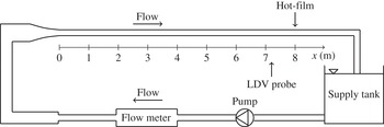
The experiments were performed in an open flow loop with water as the working fluid supplied from a 700 litre tank, as shown in figure 1. The flow was driven by an Oberdorfer N1100 gear pump and the flow rate was constantly monitored by a Krohne OPTIFLUX electromagnetic flow meter, which has an accuracy of
 $\pm$
0.7 % for the flow rates covered in the present experiments. The 10.4 m straight test section is 100 mm in diameter and consists of three flush-connected Plexiglas pipes and one 100 mm long stainless-steel pipe in which the wall shear stress probe was mounted. A
 $2:1$
contraction precedes the pipe, and the flow is tripped at the exit of the contraction to speed up the boundary layer development. The present velocity and wall friction measurements were performed at 72 and 80 pipe diameters from the inlet, respectively. Lien et al. (Reference Lien, Monty, Chong and Ooi2004) recommend, ideally, that measurements should be performed at least 150 diameters beyond the inlet to ensure fully developed conditions. However, Zagarola & Smits (Reference Zagarola and Smits1998) suggest that the entry length
 $L_{h}$
can be estimated by
 $L_{h}/D=0.5/f+5/f^{1/2}$
, where
 $f$
is the friction factor, which gives a value of
 ${\sim}$
50 (5 m) in the current set-up. Furthermore, the wall shear stress measurements presented by He et al. (Reference He, Ariyaratne and Vardy2011) showed negligible differences between adjacent measurement stations beyond 50 diameters. Based on the latter two facts, the lengths from inlet to test sections in this study were considered sufficient.
The flow rate oscillations were induced by varying the pump voltage; an in-house designed code was used to control a frequency converter, which supplied the pump with a sinusoidally varying voltage. The program enables the imposition of up to three simultaneous pulsations on the mean flow. The amplitude, frequency and phase of each pulsation can be set individually. The program sends an encoder signal at the beginning of each period such that the phase of each pulsation can be monitored separately.
Spectral analyses of the acquired signals showed that the test rig provided satisfactory stability and repeatability for the oscillating component. The measured long-time mean value of the flow rate among different days was within
 $\pm$
0.25 %.
Schematic of the experimental set-up.

2.1. Test conditions
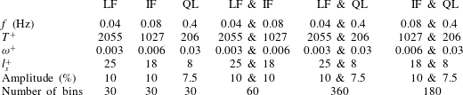
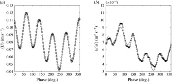
The unsteady flows covered in the study are summarized in table 1. Three types of flow conditions have been investigated: steady-state flow, single-frequency pulsating flow and double-frequency pulsating flow in which two pulsations were superimposed simultaneously on the mean flow, which resulted in a response of the velocity as illustrated in figure 3. The mean Reynolds number
 $Re=U_{b}D/{\it\nu}$
in each case was 14 500 within 0.4 %. The corresponding Kármán number
 $Re_{{\it\tau}}=\bar{u}_{{\it\tau}}D/{\it\nu}$
was 900 within 1 %. Single-frequency measurements were performed in the low-frequency, intermediate and quasi-laminar regimes at
 $l_{s}^{+}$
values of 25, 18 and 8, which correspond to absolute frequencies of 0.04, 0.08 and 0.4 Hz, respectively. The oscillation period scaled in viscous units,
 $T^{+}=T\bar{u}_{{\it\tau}}^{2}/{\it\nu}$
, corresponding to these pulsations were 2055, 1028 and 206, respectively. The steady-state value of the friction velocity has been used to calculate
 $l_{s}^{+},{\it\omega}^{+}$
and
 $T^{+}$
, but from figure 6 it follows that the scale differed by less than 0.5 % between the steady and unsteady cases and was therefore virtually identical. To simplify the post-processing, the set of pulsations was selected such that the forcing frequencies were harmonics of each other. Measurements with the simultaneous imposition of two pulsations were performed at the three combinations that can be formed from the above set, yielding seven sets of data, including the steady measurements. The pulsations were imposed with zero phase shift relative to each other. Preliminary measurements and qualitative flow visualizations revealed that the natural frequency of the test rig is close to 0.7 Hz. This required a smaller amplitude for the 0.4 Hz oscillation to reduce the effect of this pulsation. The oscillation amplitude was set to 10 % of the bulk flow rate at 0.04 and 0.08 Hz, whereas an amplitude of 7.5 % was selected for the 0.4 Hz oscillation.
Experimental conditions for the unsteady measurements. LF, IF and QL denote the low-frequency, intermediate-frequency and quasi-laminar regimes, respectively. The friction velocity, used to calculate
 $T^{+}$
,
 ${\it\omega}^{+}$
and
 $l_{s}^{+}$
, was obtained from the steady-state wall shear stress measurement. The number of bins is discussed in § 2.4.

2.2. Velocity measurements
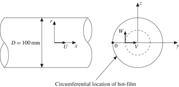
A two-component LDV system from Dantec Dynamics was used to measure the axial (
 $U$
) and tangential (
 $W$
) velocity components as shown in figure 2. The measurements were performed in the plane passing through the centreline of the pipe by traversing the measurement volumes along the
 $y$
-axis. The measurement system consisted of a 300 mW argon ion laser, transmitting optics, an 85 mm fibre probe equipped with a 310 mm focal length lens, a photodetector, a signal processor and a computer. A
 $1.98\times$
beam expander was mounted on the probe, resulting in measurement volumes of dimensions
 $(d_{x}\times d_{y}\times d_{z})=0.097~\text{mm}\times 0.85~\text{mm}\times 0.097~\text{mm}$
(
 $0.88{\it\delta}_{{\it\nu}}\times 7.60{\it\delta}_{{\it\nu}}\times 0.88{\it\delta}_{{\it\nu}}$
) and
 $(d_{x}\times d_{y}\times d_{z})=0.10~\text{mm}\times 0.91~\text{mm}\times 0.10~\text{mm}$
(
 $0.90{\it\delta}_{{\it\nu}}\times 8.17{\it\delta}_{{\it\nu}}\times 0.90{\it\delta}_{{\it\nu}}$
) in the axial and tangential directions, respectively. Here,
 ${\it\delta}_{{\it\nu}}$
denotes the viscous length scale,
 ${\it\delta}_{{\it\nu}}={\it\nu}/\bar{u}_{{\it\tau}}$
(the viscous scale at steady state has been used when presenting the dimensions in wall units). The system was used in backscattering mode and the sampling was performed in burst mode, only accepting coincident samples from the two channels occurring within 0.5 ms. This criterion was based on the diameter of the measurement volumes and the highest expected velocity of the flow.
The radial velocity (
 $V$
) is of interest to measure because it enables calculation of the turbulence production. To map this component, the measurement volumes must be traversed along the
 $z$
-axis. However, the curved surface of the pipe inhibits coincident measurements at the centreline and the refractions at the Plexiglas–water interface make it difficult to locate the positions of the measurement volumes. Because of these limitations, this component was not measured.
To reduce optical distortions from the curved surface, a rectangular glass box was mounted around the circular pipe and filled with paraffin oil (refractive index of 1.47). Different index-matching liquids were tested, and paraffin oil was found to be best among those investigated. The index matching increased the data quality, and rate, near the wall and enabled measurements at smaller
 $y^{+}~(=y/{\it\delta}_{{\it\nu}})$
.
The velocity measurements were acquired at a distance of 72 pipe diameters (7.2 m) away from the test section inlet at 36 radial positions covering
 $y^{+}$
values between 6 and 440 (the centreline). The radial movement of the probe was performed by a traverse, which could be adjusted in steps of 17
 ${\rm\mu}$
m (0.15
 ${\it\delta}_{{\it\nu}}$
) in water. At least 400 periods of oscillation were recorded at each measuring point. The data rate close to the wall was around 10 Hz, and an order of magnitude larger further out in the flow.
Definition of the coordinate system. The LDV probe was traversed along the
 $y$
-axis to measure the
 $U$
and
 $W$
components.

2.3. Wall shear stress measurements
The wall shear stress was measured with a flush-mounted 55R46 hot-film probe from Dantec. The dimensions of the measuring element are
 $0.20~\text{mm}\times 0.75~\text{mm}$
(
 $1.80{\it\delta}_{{\it\nu}}\times 6.74{\it\delta}_{{\it\nu}}$
), in the streamwise and circumferential directions, respectively. A Dantec Streamline Pro CTA system was used to control the sensor, which operated at an overheat ratio of 8 %. The probe, located 80 diameters (8 m) away from the pipe inlet, was mounted in a 100 mm long metal pipe to enable liquid grounding close to the probe.
The sensor was calibrated in situ by varying the Reynolds number between 6000 and 28 000 while recording the flow rate and hot-film voltage. The wall shear stress at each Reynolds number was calculated from
 ${\it\tau}=({\it\rho}U_{b}^{2}f)/8$
, where
 ${\it\rho}$
and
 $f=0.3164\mathit{Re}^{-1/4}$
are the fluid density and the friction factor, respectively. The friction factor was extracted from the semi-empirical Blasius formula (see Pope Reference Pope2000). More accurate formulas, such as Prandtl’s friction law for smooth pipes (see Pope Reference Pope2000), exist to determine the friction factor. For the Reynolds numbers encountered in this study, the Blasius relation agrees with Prandtl’s friction law within 3 %. The Blasius relation was used because its explicit formulation enables derivation of quasi-steady asymptotes for low-frequency pulsations. In principle, a higher accuracy can be achieved by calibrating the sensor versus the pressure drop
 ${\rm\Delta}p$
over the length
 $L$
,
 ${\it\tau}={\rm\Delta}pD/4L$
. This approach does not involve estimating the friction factor, and the wall shear stress is proportional to the first power of each quantity. When the wall shear stress is calculated from the flow rate, the dependences on the pipe diameter and flow rate are of the fourth and second powers, respectively. This high-order power-law relationship causes a great sensitivity to propagation of errors in these quantities. However, the small differential pressure gradients encountered in the current experimental set-up (
 $\text{d}p/\text{d}x\sim 1{-}10~\text{Pa}~\text{m}^{-1}$
) could not be measured with sufficient accuracy; thus, the sensor was calibrated versus the flow rate. The estimated values of the wall shear stress were fitted to the measured hot-film voltage,
 $E$
, by the Lévêque solution (see Goldstein Reference Goldstein1996)
 $$\begin{eqnarray}{\it\tau}^{1/3}=A+BE^{2},\end{eqnarray}$$
where
 $A$
and
 $B$
are calibration constants. The sensor was calibrated before and after each measurement. Satisfactory performance of the hot-film was assured by inspecting the normalized r.m.s. values. These were scattered around 0.37, which agrees with the value of 0.4 reported in the extensive experimental study of the fluctuating wall shear stress performed by Alfredsson et al. (Reference Alfredsson, Johansson, Haritonidis and Eckelman1988).
The hot-film signal was acquired using a PXI system consisting of a 24-bit (NI-4472) card equipped with an anti-aliasing filter. A sampling frequency of 1 kHz was selected for the present measurements. At least 1500 periods were recorded to assure converged results.
2.4. Data reduction
Owing to the periodic nature of the flow, a Reynolds triple decomposition as described by Telionis (Reference Telionis1981) was used to post-process the data. Any acquired flow quantity
 ${\it\varphi}$
at radius
 $r$
, phase
 ${\it\theta}$
and time
 $t$
was decomposed into its mean value, periodic component and turbulent fluctuation:
 $$\begin{eqnarray}{\it\varphi}(r,{\it\theta},t)=\bar{{\it\varphi}}(r)+\widetilde{{\it\varphi}}(r,{\it\theta})+{\it\varphi}^{\prime }(r,t),\end{eqnarray}$$
where
 $\bar{{\it\varphi}}$
,
 $\widetilde{{\it\varphi}}$
and
 ${\it\varphi}^{\prime }$
denote the time average, periodic/oscillating/modulation component and turbulent fluctuation, respectively. In subsequent sections, the time-averaged velocity is represented by an upper-case letter with a bar, the periodic component is represented by an upper-case letter with a tilde, and the turbulent fluctuation is written with a primed lower-case letter. For the wall shear stress, the convention introduced in (2.2) is used to distinguish the different components. The phase, or ensemble, average is defined as the sum of the time average and the periodic component:
 $$\begin{eqnarray}\langle {\it\varphi}(r,{\it\theta})\rangle \equiv \bar{{\it\varphi}}(r)+\widetilde{{\it\varphi}}(r,{\it\theta})=\frac{1}{N}\mathop{\sum }_{i=1}^{N}{\it\varphi}(r,{\it\theta}+i{\it\omega}T),\end{eqnarray}$$
where
 $N$
is the number of recorded cycles, each of period time
 $T$
. From (2.2) and (2.3), the ensemble-averaged turbulent fluctuation is defined as
 $\langle {\it\varphi}^{\prime }{\it\varphi}^{\prime }\rangle \equiv \overline{{\it\varphi}^{\prime }{\it\varphi}^{\prime }}+\widetilde{{\it\varphi}^{\prime }{\it\varphi}^{\prime }}=\langle {\it\varphi}^{2}\rangle -\langle {\it\varphi}\rangle ^{2}$
. For double-frequency flow, the system is forced by the superposition of two sinusoids. The period of the resulting signal equals that of the slowest pulsation, which, consequently, has been used for phase averaging in those cases. The mean values and the turbulent fluctuations were calculated through weighted averaging:
 $$\begin{eqnarray}\left.\begin{array}{@{}c@{}}\displaystyle \bar{{\it\varphi}}=\mathop{\sum }_{i=1}^{M}{\it\eta}_{i}{\it\varphi}_{i},\\ \displaystyle \overline{{\it\varphi}^{\prime 2}}=\mathop{\sum }_{i=1}^{M}{\it\eta}_{i}({\it\varphi}_{i}-\bar{{\it\varphi}})^{2},\end{array}\right\}\end{eqnarray}$$
where
 $M$
is the total number of samples, and
 ${\it\eta}_{i}$
equals
 $1/M$
(arithmetic weighting) for the wall shear stress data and
 ${\it\xi}_{i}/\sum _{j=1}^{M}{\it\xi}_{j}$
(transit time weighting) for the LDV data. Each velocity sample was weighted with its transit time
 ${\it\xi}$
through the measurement volume to reduce the velocity bias error (see Mulu Reference Mulu2012).
Close to the wall (
 $y^{+}<20$
), large velocity gradients prevail, which causes significant velocity variations across the finite size of the measurement volume. This variation affects the velocity measurements, and to overcome this problem the axial LDV measurements were corrected for the velocity gradient bias as proposed by Durst et al. (Reference Durst, Martinuzzi, Sender and Thevenin1992):
 $$\begin{eqnarray}\left.\begin{array}{@{}c@{}}\overline{U}_{m}=\overline{U}_{t}+\displaystyle \frac{l^{2}}{32}\left(\frac{\text{d}^{2}\overline{U}_{t}}{\text{d}y^{2}}\right)+\text{h.o.t.},\\ \overline{u_{m}^{\prime 2}}=\overline{u_{t}^{\prime 2}}+\displaystyle \frac{l^{2}}{16}\left(\frac{\text{d}\overline{U}_{t}}{\text{d}y}\right)^{2}+\text{h.o.t.},\end{array}\right\}\end{eqnarray}$$
where
 $l$
is the length of the measurement volume in the direction of the gradient, indices
 $m$
and
 $t$
represent the measured and true values, respectively, and h.o.t. represents higher-order terms. To reduce the noise that occurs when discrete measurement data are differentiated, the velocity profiles were smoothed before calculation of the derivatives in (2.5). Piecewise quadratic curve fits were applied to eight consecutive points, and the velocity gradient was calculated from the resulting curve fit. Despite the curve fitting, a residual level of noise remained, which required further smoothing by applying a similar curve-fitting procedure on the calculated gradients. Equation (2.5) was initially derived to correct biased mean values in steady flow. In this work, (2.5) was also applied in each bin to correct the phase-averaged quantities in unsteady flow. Successful extension of these equations to unsteady flows was assured by the similarity between
 $\overline{u_{t}^{\prime 2}}$
calculated from the time-averaged data and the time average of
 $\langle u_{t}^{\prime 2}\rangle$
. The correction term for
 $\overline{U}_{m}$
and
 $\langle U_{m}\rangle$
was small, generally below 5 %. The estimated uncertainty for the second-order derivative in (2.5) was
 $\pm$
8 %; thus, the uncertainty of the calculated derivative was greater than the correction term. Therefore,
 $\overline{U}_{m}$
and
 $\langle U_{m}\rangle$
were not corrected. Close to the wall, the corrections for
 $\overline{u_{m}^{\prime 2}}$
and
 $\langle u_{m}^{\prime 2}\rangle$
were up to 30 % and 60 % of the measured value, respectively, and thus of great importance. Similar conclusions were drawn by Durst et al. (Reference Durst, Martinuzzi, Sender and Thevenin1992), who showed that the gradient bias primarily affects the turbulent fluctuations whereas the mean velocity profile and higher-order moments are less influenced by the gradient bias.
At the beginning of each oscillation cycle, an encoder signal was sent to the data acquisition systems, which allowed the acquired data to be transposed onto a single period. The period was subdivided into bins of equal size
 ${\rm\Delta}{\it\theta}$
, centred at
 ${\it\theta}_{0}$
. The number of phase bins was dependent on the case under consideration as shown in table 1. For instance, the rapid oscillations at the combination of pulsations of 0.08 and 0.4 Hz (see figure 3) required 180 phase bins to accurately capture the oscillations. In single-frequency pulsating flow, 30 bins were sufficient to obtain converged results while still reproducing the phase average. The phase average was calculated by extracting the mean value of the desired quantity in each bin. The Fourier series of each phase-averaged quantity,
 $$\begin{eqnarray}\langle {\it\varphi}(n)\rangle =\mathop{\sum }_{k=0}^{N-1}{\it\Phi}(k)\text{e}^{\text{i}2{\rm\pi}k(n/N)},\end{eqnarray}$$
was calculated and used to post-process the acquired data. The phase-averaged quantities presented in the results section were extracted from the fundamental mode in the case of single-frequency flow, and, respectively, the fundamental mode and current harmonic in double-frequency flow. The phase-averaged velocity and wall shear stress were accurately described by these modes and generally contained more than 99 % of the power spectral density. Larger deviations were observed for the turbulent fluctuations, particularly in the outer part of the flow where the fluctuations are small; see figure 10(a). At these points, the power spectral density of the Fourier modes could be as low as 10 %, but closer to the wall, the corresponding number was around 90 %. Examples of profiles of the phase-averaged velocity and turbulent fluctuations are shown on figure 3.
Example of phase-averaged velocity (a) and turbulent velocity fluctuations (b) from LDV measurements;
 $l_{s}^{+}=18$
and 8,
 $y^{+}=11$
. Symbols, measured data; solid line, sum of fundamental mode and fifth harmonic from Fourier series (2.6).

2.5. Uncertainty analysis
2.5.1. Velocity measurements
The main bias errors of the velocity measurements derived from the velocity bias error and the calibration factor
 ${\it\delta}_{f}={\it\lambda}/(2\sin {\it\beta})$
, where
 ${\it\lambda}$
is the laser wavelength and
 ${\it\beta}$
the beam half-angle. The laser was aimed at a distant wall and the spacing between the beams was measured to determine the half-angle. From a Monte Carlo simulation, the uncertainty of the calibration factor was determined to
 $\pm$
1 %. The uncertainty from the velocity bias error was estimated to
 $\pm$
0.7 % by calculating the difference between the corrected and uncorrected values
 $b_{vb}^{2}=(\overline{U}-(1/N)\sum _{i}U_{i})^{2}$
(see Mulu Reference Mulu2012). The random error was assessed to
 $\pm$
0.65 % by calculating the standard deviation of the mean values from repeated runs of the steady-state measurements. The overall uncertainty of the velocity measurements at the 95 % confidence level was therefore
 $\pm 2\sqrt{1^{2}+0.65^{2}+0.7^{2}}=\pm 2.5\,\%$
.
2.5.2. Wall shear stress measurements
The uncertainty of the calculated wall shear stress was assessed by expanding a 95 % confidence interval around the calibration curve defined by (2.1). The errors involved in determining the calibration curve with corresponding uncertainty intervals are composed of two parts: (i) the estimation of
 ${\it\tau}$
and (ii) the uncertainties in the hot-film voltage. The main sources of uncertainties when estimating the wall shear stress are related to the inaccuracies of the friction factor, the flow rate and the pipe diameter. The random error of the estimated wall shear stress resulted from the inaccuracies of the flow meter and the inability to reach repeatable conditions. The random error varied between 0.3 % and 0.8 %, with larger uncertainties occurring at lower Reynolds numbers because of the lower accuracy of the flow meter for small flow velocities. The corresponding systematic error was estimated to be 3.2 %. The main sources of errors in the measured hot-film voltage were related to the mounting of the sensor and drifting of the calibration curve due to contamination of the sensor and changes in the water temperature. Sensitivity analyses of the hot-film voltage dependence of the water temperature and frequent updating of the calibration curve led to an estimate of the random error of the hot-film voltage within
 $\pm$
0.6 %. The systematic error was estimated to 1.8 %. From the uncertainties presented above and the method of propagating uncertainties to calibration curves derived by Coleman & Steele (Reference Coleman and Steele2009), the final uncertainty at the 95 % confidence level of the measured wall shear stress used from (2.1) was
 $\pm$
13 %.
3. Results and discussion
The results section is divided into two main parts: time-averaged and phase-averaged quantities. The experiments from single-frequency and double-frequency pulsating flow are referred to as cases I and II, respectively. A (
 $+$
) superscript denotes variables scaled with the time-averaged viscous scales and an (s) subscript denotes scaling with the Stokes length. At a few occasions the notation
 $u_{i}^{\prime }$
is used in which
 $i=1,2$
, i.e.
 $u_{1}^{\prime }=u^{\prime }$
and
 $u_{2}^{\prime }=w^{\prime }$
.
3.1. Time-averaged quantities
3.1.1. Mean velocity profiles
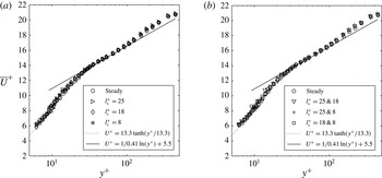
Figure 4(a,b) shows the time-averaged axial velocity in cases I and II, respectively. The data are presented in wall units, i.e.
 $\overline{U}^{+}$
versus
 $y^{+}$
. No measurements were performed in the region in which
 $\overline{U}^{+}=y^{+}$
, which introduced ambiguity to determine the exact position of the velocity profile along the abscissa. To overcome this issue, the residuals of the steady-state velocity measurements up to
 $y^{+}=14$
were minimized with respect to the curve
 $\overline{U}^{+}=13.3\,\text{tanh}(y^{+}/13.3)$
. This curve was obtained from a least-squares fit of the pipe flow LDV measurements (
 $Re=7442$
) in the region
 $1<y^{+}<14$
presented in Durst, Jovanovic & Sender (Reference Durst, Jovanovic and Sender1995). The data of Durst et al. (Reference Durst, Jovanovic and Sender1995) are in close agreement with the pipe flow DNS (
 $Re=11\,700$
) of El Khoury et al. (Reference El Khoury, Schlatter, Noorani, Fischer, Brethouwer and Johansson2013), which justifies the use of these data as a reference for locating the position of the measurement volume in the present measurements. The uncertainty of the position of the measured profile along the abscissa is
 $\pm {\it\delta}_{{\it\nu}}/2$
, considering the accuracy of the LDV measurements and the precision of the traverse. In addition to the time-averaged profiles from the unsteady measurements, the steady-state measurements, the curve
 $\overline{U}^{+}=13.3\,\text{tanh}(y^{+}/13.3)$
and the log law with
 ${\it\kappa}=0.41$
and
 $B=5.5$
are plotted as reference data. Despite some scatter, all points collapse onto the same curve, showing that the mean velocity is insensitive to the imposed pulsations; their profiles are similar to the reference data.
Time-averaged axial velocity profiles: (a) case I, (b) case II. The dotted line is covered by the experimental data for
 $y^{+}>6$
.

3.1.2. Mean turbulence profiles
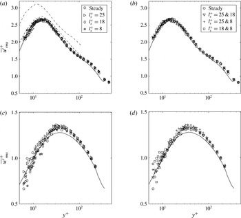
Figure 5(a–d) presents the time-averaged r.m.s. turbulent velocity fluctuations
 $\overline{u^{\prime }}_{i,rms}^{+}$
, data from the steady pipe flow DNS performed by El Khoury et al. (Reference El Khoury, Schlatter, Noorani, Fischer, Brethouwer and Johansson2013) and the results from the pulsating channel flow LES at
 $l_{s}^{+}=7,14$
and 35 by Scotti & Piomelli (Reference Scotti and Piomelli2001). As observed for the mean velocity, the time-averaged turbulence profiles from the steady and unsteady cases are similar, with no sign of the imposed pulsations. For the axial component, the peak value of approximately 2.6 at
 $y^{+}\approx 14$
is in excellent agreement with the DNS. When
 $y^{+}>100$
, the measured profiles start to diverge from the DNS because of the difference in Reynolds number between the studies (see Durst et al.
Reference Durst, Jovanovic and Sender1995). For the LES, the data closely overlap the present results at the highest pulsation but
 $\overline{u^{\prime }}_{rms}^{+}$
increases systematically with
 $l_{s}^{+}$
, and for
 $l_{s}^{+}=35$
, the peak value is approximately 15 % larger and has moved towards the wall. As discussed in § 1, the increased turbulence level is probably attributable to a larger turbulence production, stemming from the additional term
 $-\overline{\widetilde{u^{\prime }v^{\prime }}\partial \widetilde{U}/\partial y}$
in the transport equation for
 $\overline{u^{\prime 2}}$
, which becomes effective for large-amplitude, low-frequency, oscillations. Closer inspection shows that the peak value and the location of the peak are offset by roughly equal amounts. Thus, part of the difference can be attributed to scaling effects. As will be discussed in § 3.1.3, the mean wall shear stress can be expected to increase for low-frequency, large-amplitude, oscillations. The LES were however performed with a fixed mean pressure gradient, and thus at a fixed mean wall shear. The data were rescaled (not shown) with this expected increase taken into account. A closer collapse was achieved but, as observed in figure 5(a), the offset for
 $l_{s}^{+}=35$
is not constant and the phenomenon is thus more complicated than a matter of scaling.
Time-averaged r.m.s. velocity fluctuations: (a,c) case I, (b,d) case II. Steady pipe flow DNS by El Khoury et al. (Reference El Khoury, Schlatter, Noorani, Fischer, Brethouwer and Johansson2013),
 $Re=11\,700$
: solid line. Channel flow LES by Scotti & Piomelli (Reference Scotti and Piomelli2001): dotted,
 $l_{s}^{+}=7$
; dashed,
 $l_{s}^{+}=14$
; dashed-dotted,
 $l_{s}^{+}=35$
.

Close to the wall, the data of the tangential component display a larger scatter than the axial counterpart but the profiles from the unsteady cases are not appreciably different from the steady measurements. The measured peak values are slightly larger than that from the DNS, but
 $\overline{w^{\prime }}_{rms}^{+}$
showed a significant dependence upon the Reynolds number in the DNS (performed at
 $Re=5300,~11\,700,~19\,000$
and 37 700) and the experimental data fall midway between the plotted curve (
 $Re=11\,700$
) and the one at
 $Re=19\,000$
.
The relative turbulence intensity
 $\overline{u^{\prime }}_{rms}/\overline{U}$
(the steady profile of which is plotted on figure 10
e) collapses onto a single curve for all investigated cases. The intensity increases in the radial direction and the measurement closest to the wall (
 $y^{+}=6$
) attains a value of
 ${\sim}$
0.35. The profiles converge towards an asymptotic constant value between 0.35 and 0.4, as expected, because both the turbulent fluctuations and the mean velocity grow linearly with
 $y$
close to the wall. The asymptotic turbulence intensity agrees well with the pipe flow DNS (
 $Re=5300$
) performed by Eggels et al. (Reference Eggels, Unger, Weiss, Westerweel, Adrian, Friedrich and Nieuwstadt1994), and the measured r.m.s. wall shear stress fluctuations presented in figure 6(b), which are randomly scattered around 0.37.
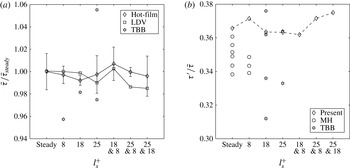
Time-averaged wall shear stress in steady and unsteady flows: (a) mean values and (b) r.m.s. turbulent fluctuations from hot-film measurements. The steady hot-film value has been used for normalization in (a). The error bars in (a) denote one standard deviation from the hot-film measurements. MH, data from Mao & Hanratty (Reference Mao and Hanratty1986); TBB, data from Tardu et al. (Reference Tardu, Binder and Blackwelder1994).

3.1.3. Mean wall shear stress and turbulent fluctuations
The steady-state, case I and case II time-averaged wall shear stress, measured with the hot-film sensor and estimated from the LDV data, is plotted in figure 6(a). The time-averaged LDV measurements in the logarithmic region (taken to be
 $30<y^{+}<100$
) were used to calculate the value of
 $\bar{u}_{{\it\tau}}$
that yielded the optimum fit to the log law with
 ${\it\kappa}=0.41$
and
 $B=5.5$
assumed to hold. The wall shear stress was subsequently calculated from
 $\bar{{\it\tau}}={\it\rho}\bar{u}_{{\it\tau}}^{2}$
. The procedure of calculating the wall shear stress from the velocity was performed, not to determine
 ${\it\kappa}$
and
 $B$
, nor to investigate the existence of a universal overlap region, but merely as a means of comparison. The hot-film measurements were repeated five times at each operating point and the average of these repetitions has been used for the presented data. The error bars denote one standard deviation. To assess the repeatability of the wall shear stress measurements from the velocity data, the steady-state LDV measurements were repeated three times in the logarithmic region and displayed a similar scatter.
The two sets of measurements are in close agreement, with the largest deviation between the methods within 1.5 %. Furthermore, no trend is seen between the cases; the case I and the case II data are scattered within
 $\pm$
1 % of the steady value. These results are somewhat different from those presented in Tardu & Binder (Reference Tardu and Binder1993) and Tardu et al. (Reference Tardu, Binder and Blackwelder1994), in which the mean wall shear stress showed a larger scatter. Their data fell between
 $+$
14 % and
 $-$
9 % around the steady value, although the subset plotted in figure 6(a) displays a smaller scatter. At large oscillation amplitudes, the deviations from the steady value were argued to originate from a nonlinear interaction between the oscillating flow and the mean flow. By assuming that the Blasius friction formula holds at each instant of the oscillation cycle, Tardu et al. (Reference Tardu, Binder and Blackwelder1994) derived an expression for the mean wall shear stress in the quasi-steady regime:
 $\bar{{\it\tau}}_{qs}=\bar{{\it\tau}}_{steady}(1+(21/64)a_{\widetilde{U}_{c}}^{2})$
. In their study, the maximum value of the normalized centreline velocity oscillations,
 $a_{\widetilde{U}_{c}}=A_{\widetilde{U}_{c}}/\overline{U}_{c}$
, was 0.7. This corresponds to a 16 % larger mean wall shear stress compared to the steady case and is in good agreement with the maximum value measured in their study. However, the scatter in their data was quite significant and showed no definite trend of increasing values of the time-averaged wall shear stress at large amplitudes. In the present study,
 $a_{\widetilde{U}_{c}}\approx 0.13$
, which results in a correction term
 ${<}$
1 %, thus suggesting that the nonlinearity is negligible.
The normalized r.m.s. turbulent fluctuations (
 ${\it\tau}^{\prime }/\bar{{\it\tau}}$
) are plotted in figure 6(b). The data are scattered between 0.36 and 0.38, in agreement with the limiting value of the close-wall LDV measurements. Data from Mao & Hanratty (Reference Mao and Hanratty1986) and Tardu et al. (Reference Tardu, Binder and Blackwelder1994) at similar values of
 $l_{s}^{+}$
have been included in the figure. The multiple data points stem from different combinations of frequencies and Reynolds numbers. The scatter in their data is quite large, and the r.m.s. fluctuations are generally smaller than 0.36. However, recent hot-film measurements in transient pipe flows performed by He et al. (Reference He, Ariyaratne and Vardy2011) found a steady-state value of 0.38. Furthermore,
 ${\it\tau}^{\prime }/\bar{{\it\tau}}$
is a weak function of the Reynolds number (see Durst et al.
Reference Durst, Jovanovic and Sender1995) and usually displays scatter among different studies due to the experimental difficulties involved when measuring this quantity. Consequently, the conclusion to be drawn from the present data is that
 ${\it\tau}^{\prime }/\bar{{\it\tau}}$
is unaffected by small-amplitude pulsations.
3.2. Phase-averaged quantities
3.2.1. Amplitude and phase of the oscillating velocity
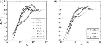
The amplitudes of the streamwise oscillating velocity in cases I and II are plotted in figure 7(a,b). The results are plotted versus the wall-normal coordinate normalized with the Stokes length
 $y_{s}~(=y/l_{s})$
to enable comparison with the analytical laminar solutions derived by Uchida (Reference Uchida1956):
 $$\begin{eqnarray}\widetilde{U}=\mathop{\sum }_{n}A_{\widetilde{U}_{c_{n}}}\text{Re}\left[\text{i}\left(\frac{\text{J}_{0}(\text{i}^{3/2}\sqrt{2}r/l_{s_{n}})}{\text{J}_{0}(\text{i}^{3/2}\sqrt{2}R/l_{s_{n}})}-1\right)\text{e}^{\text{i}{\it\omega}_{n}t}\right].\end{eqnarray}$$
In (3.1),
 $\text{J}_{0}$
is the Bessel function of order zero and the first kind;
 $A_{\widetilde{U}_{c_{n}}}$
,
 $l_{s_{n}}$
and
 ${\it\omega}_{n}$
are the
 $n$
th mode of the amplitude of the centreline velocity, the laminar Stokes length and the angular frequency, respectively; in case I,
 $n=1$
, and in case II,
 $n=\{1,2;1,5;1,10\}$
;
 $\text{Re}[\cdots ]$
denotes the real part of the argument;
 $\text{i}=\sqrt{-1}$
is the imaginary unit; and
 $R$
is the pipe radius. Near the wall, (3.1) is approximately given by
 $$\begin{eqnarray}\widetilde{U}\approx \mathop{\sum }_{n}A_{\widetilde{U}_{c_{n}}}[\text{sin}({\it\omega}_{n}t)-\text{e}^{-y/l_{s_{n}}}\text{sin}({\it\omega}_{n}t-y/l_{s_{n}})],\end{eqnarray}$$
where the wall-normal coordinate
 $y=R-r$
is introduced to match the coordinate system in figure 2.
Amplitude of the oscillating velocity normalized with the centreline value for (a) case I and (b) case II. The solid, dotted and dashed lines in (b) are the laminar Stokes solutions for the combination of a fundamental mode along with its tenth, fifth and second harmonic, respectively. HJ, data from He & Jackson (Reference He and Jackson2009).

Phase difference relative to the oscillating centreline velocity: (a) case I, (b) individual modes from case II. In (b), only one set of data has been included to increase the readability. HJ, data from He & Jackson (Reference He and Jackson2009).

In case I, the amplitude profile for
 $l_{s}^{+}=8$
plotted in figure 7(a) follows the Stokes solution fairly well, although the measured peak amplitude is smaller than the laminar value and attained at a larger
 $y_{s}$
. For
 $y_{s}>6$
, the velocity oscillates as a plug, similar to the Stokes solution. The thickened oscillating boundary layer indicates that turbulence diffuses the shear wave generated at the wall, thereby supporting the similarity parameter
 $l_{t}^{+}$
proposed by Scotti & Piomelli (Reference Scotti and Piomelli2001); see § 1. The thickening of the oscillating boundary layer is also displayed in the phase difference,
 ${\it\phi}_{\widetilde{U}}-{\it\phi}_{\widetilde{U}_{c}}$
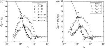
, with the local minimum displaced by approximately two Stokes units into the core; see figure 8(a).
The results from the intermediate regime (
 $l_{s}^{+}=18$
) are consistent with the findings of previous studies (see Tardu & Binder Reference Tardu and Binder1993; Tardu et al.
Reference Tardu, Binder and Blackwelder1994; Scotti & Piomelli Reference Scotti and Piomelli2001). Near the wall for
 $y_{s}<1$
, the amplitude of the oscillating velocity follows the Stokes solution, although the flow is no longer in the quasi-laminar regime. Because the oscillating wall shear stress is given by
 $\widetilde{{\it\tau}}={\it\mu}\,\partial \widetilde{U}/\partial y$
, the observed behaviour indicates that the turbulence decreases the oscillating shear in this regime. This phenomenon will be discussed thoroughly in § 3.2.3, in which the measurements of the oscillating wall shear stress are presented.
A feature of the amplitude of the oscillating velocity in the intermediate and the low-frequency regimes (
 $l_{s}^{+}=18$
and
 $l_{s}^{+}=25$
) is that the amplitude profiles display similarities to the time-averaged velocity plotted on figure 4. For
 $y_{s}>2$
, i.e. when the direct effect of molecular viscosity is small, a logarithmic region exists in which the slopes of the two curves are linear. The normalized Stokes length;
 $l_{s}^{+}=l_{s}\bar{u}_{{\it\tau}}/{\it\nu}$
can be interpreted as a Reynolds number for the oscillating flow, and for sufficiently large
 $l_{s}^{+}$
(say
 $l_{s}^{+}>15$
), features of the oscillating flow similar to the time-averaged flow could be expected. For
 $y_{s}>2$
and sufficiently far from
 $R_{s}~(=R/l_{s})$
, dimensional reasoning leads to
 $\text{d}\widetilde{U}/\text{d}y=C\widetilde{U}_{c}/y$
. Integrating this expression results in
 $\widetilde{U}/\widetilde{U}_{c}=C\,\text{ln}(y)+D$
, where
 $C$
and
 $D$
are constants that depend on
 $l_{s}^{+}$
. The onset of the logarithmic velocity distribution is accompanied by a reversal of
 ${\it\phi}_{\widetilde{U}}-{\it\phi}_{\widetilde{U}_{c}}$
; see figure 8(a). For
 $y_{s}<2$
, the phase shift increases linearly on a semi-logarithmic scale whereas
 ${\it\phi}_{\widetilde{U}}-{\it\phi}_{\widetilde{U}_{c}}$
decreases at a nearly equal rate for
 $y_{s}>2$
. Amplitude and phase data at similar values of
 $l_{s}^{+}$
from the pipe flow study (
 $Re=7000$
) by He & Jackson (Reference He and Jackson2009) have been included in figures 7(a) and 8(a). The general trends are qualitatively similar to the present results but quantitatively there are disparities, especially in the phase difference. As for the phase difference, for
 $l_{s}^{+}\gtrsim 15$
, a local maximum of
 ${\it\phi}_{\widetilde{U}}-{\it\phi}_{\widetilde{U}_{c}}$
at
 $y_{s}\approx 2$
is also displayed in the data reported by Tardu et al. (Reference Tardu, Binder and Blackwelder1994) and Cervantes & Engstrom (Reference Cervantes and Engstrom2008) among others, but the peak value does not seem to scale in a simple way with
 $l_{s}^{+}$
.
The wall-normal development of the amplitude of the oscillating velocity in case II is plotted in figure 7(b) together with the corresponding Stokes solutions. The amplitude of the experimental and the analytical data in this figure is defined as
 $A_{\widetilde{U}}=(\max (\widetilde{U})-\min (\widetilde{U}))/2$
. The longest period of oscillation has been used to define the Stokes length because it is the shortest common period among the pulsations. The
 $l_{s}^{+}=25$
and 8 profile appear similar to the profile for
 $l_{s}^{+}=25$
from case I displaced vertically and with a smaller slope in the logarithmic region. The smaller slope can be explained by considering the normalized amplitude at this combination, approximately given by
 $(A_{8}+A_{25})/(A_{8_{c}}+A_{25_{c}})$
, where the numerator terms are the amplitudes at any wall-normal coordinate,
 $y_{s}$
, and the terms in the denominator are the centreline amplitudes. For
 $y^{+}>16$
,
 $A_{8}\approx A_{8_{c}}$
and the amplitude profile becomes
 $K+A_{25}/(A_{8_{c}}+A_{25_{c}})$
, where
 $K$
is a constant and the second term grows with
 $y_{s}$
, i.e. this profile resembles a displaced
 $l_{s}^{+}=25$
profile with a smaller slope in the logarithmic region. In fact, to a good approximation, the general shape of all case II profiles can be obtained by superposing the profiles from case I. For
 $y_{s}<0.6$
, the two profiles with a pulsation at
 $l_{s}^{+}=8$
follow the Stokes solutions fairly well, whereas the data at the combination
 $l_{s}^{+}=25$
and 18 diverge from the analytical solution. The same trend is displayed by the wall shear stress measurements presented in § 3.2.3. This does not, however, imply that the harmonic at
 $l_{s}^{+}=25$
tends towards the Stokes solution at the combination
 $l_{s}^{+}=25$
and 8 (see figure 9(a) and the discussion in the next paragraph). Rather, the resemblance to the analytical curve is the result of a favourable addition of amplitudes (with respect to the Stokes solution).
To further discern whether the pulsations interact when combined or whether the Fourier harmonics in case II are a superposition of the responses from case I, the fundamental mode in addition to either the
 $n=2$
, 5 or 10 harmonic were extracted from the respective Fourier series defined in (2.6). The amplitude profiles of the individual harmonics from case II,
 $l_{s_{IND}}^{+}$
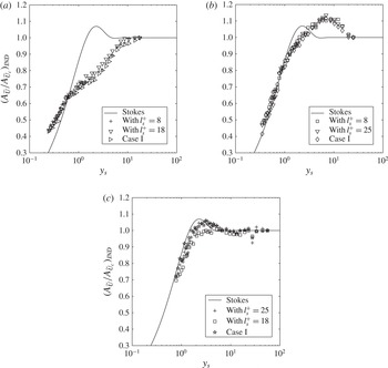
, are plotted on figure 9(a–c) along with the case I profiles. Despite some scatter, the harmonics from case II for
 $l_{s_{IND}}^{+}=25$
and
 $l_{s_{IND}}^{+}=18$
are similar to the case I profiles, regardless of the combination of pulsations. The response of the oscillating velocity for
 $l_{s_{IND}}^{+}=8$
on the other hand is slightly dependent on which pulsations are combined. For
 $l_{s}^{+}=25$
and 8, the
 $l_{s_{IND}}^{+}=8$
profile is similar to a displaced Stokes solution, whereas it deviates slightly from the laminar profile when
 $l_{s}^{+}=18$
and 8 are imposed simultaneously. The phase difference of the individual harmonics from case II,
 $({\it\phi}_{\widetilde{U}}-{\it\phi}_{\widetilde{U}_{c}})_{IND}$
, is plotted on figure 8(b). As for the oscillating velocity, two sets of data from case II are available for each value of
 $l_{s_{IND}}^{+}$
but only one set is displayed in the figure because of the similarity between the results. Only small deviations from case I are seen for
 $l_{s_{IND}}^{+}=18$
and
 $l_{s_{IND}}^{+}=25$
, whereas the data for
 $l_{s_{IND}}^{+}=8$
are more scattered around the case I values. However, the profile for
 $l_{s_{IND}}^{+}=8$
is the fifth harmonic, and any errors in locating the phase of this pulsation imply a five-fold amplification of the error in the calculated phase difference.
Oscillating velocity amplitude of individual modes from case II: (a)
 $l_{s_{IND}}^{+}=25$
, (b)
 $l_{s_{IND}}^{+}=18$
and (c)
 $l_{s_{IND}}^{+}=8$
. The data from case I have been included as reference along with the Stokes solution.

3.2.2. Amplitude and phase of the oscillating turbulent fluctuations
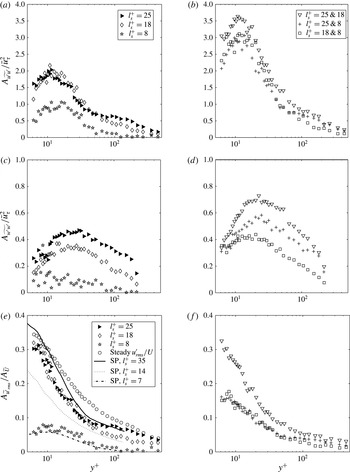
Figure 10 shows the development of the amplitude of the turbulent velocity fluctuations along the wall-normal coordinate from the two sets of unsteady measurements. The data have been scaled in two ways: (i) with the mean friction velocity and (ii) with the local oscillating velocity.
Amplitudes of the modulation of the axial and tangential turbulent velocity fluctuations: (a,c,e) case I, (b,d,f) case II. (a–d) Scaled with the mean friction velocity. (e–f) Turbulence intensity with respect to local velocity amplitude. SP, data from Scotti & Piomelli (Reference Scotti and Piomelli2001).

The modulation amplitudes scaled with the friction velocity
 $(A_{\widetilde{u_{i}^{\prime }u_{i}^{\prime }}}/\bar{u}_{{\it\tau}}^{2})$
from case I are plotted on figure 10(a,c). The profiles of the axial component are similar to the time-averaged streamwise velocity fluctuations, with peak amplitudes near
 $y^{+}=14$
, although, in spite of the scatter in the data, it appears that the peak value moves towards the wall with increasing
 $l_{s}^{+}$
. The peak amplitude is smaller than the time-averaged value because of the small amplitude of the imposed oscillations. The profiles do not exhibit a monotonic trend function of the forcing frequency; the largest peak value is attained for
 $l_{s}^{+}=18$
, and the smallest for
 $l_{s}^{+}=8$
. The difference between the peak values for
 $l_{s}^{+}=18$
and
 $l_{s}^{+}=25$
is small, however. The turbulence level for
 $l_{s}^{+}=8$
is significantly lower than at the other two frequencies because of the small Stokes length at this frequency. As a result, most of the shear generated at the wall is attenuated in the viscous sublayer, which inhibits interactions with the steady turbulence field. For
 $y^{+}>100$
, the amplitude is almost zero, i.e. the modulation of turbulence is frozen. The low turbulence level at
 $l_{s}^{+}=8$
is displayed even more clearly in the profile of the tangential component. Here, the amplitude is small along the entire radius, and, as for the axial component, the modulation is zero for
 $y^{+}>100$
. At the two lower pulsation frequencies, the profiles are similar to their steady counterparts, but again of smaller magnitude. The amplitudes of the oscillating turbulent fluctuations in case II,
 $A_{\widetilde{u_{i}^{\prime }u_{i}^{\prime }}}=(\max (\widetilde{u_{i}^{\prime }u_{i}^{\prime }})-\min (\widetilde{u_{i}^{\prime }u_{i}^{\prime }}))/2$
, are plotted on figure 10(b,d). For both the axial and the tangential components, the amplitudes are nearly the addition of the amplitudes from case I when one pulsation is at
 $l_{s}^{+}=8$
; the same is not true at the combination
 $l_{s}^{+}=25$
and 18. This follows from two arguments. (i) As for the oscillating velocity plotted on figure 9(a–c), the amplitudes of the turbulent fluctuations of the individual harmonics in case II are negligibly different from the case I amplitudes. (ii) A sinusoid and its fifth harmonic as well as a sinusoid and its tenth harmonic are close to peak at a common phase; the same is not true for a sinusoid and its second harmonic. These phase relationships are closely retained for the turbulent fluctuations all the way from the near-wall region to the centreline. Consequently, the profiles plotted on figure 10(b,d) are observed.
The modulation of the turbulent velocity fluctuations scaled with the local oscillating velocity
 $(A_{\widetilde{u^{\prime }}_{rms}}/A_{\widetilde{U}})$
from case I is plotted in figure 10(e) along with the steady-state profile (
 $\overline{u^{\prime }}_{rms}/\overline{U}$
) and the LES data from Scotti & Piomelli (Reference Scotti and Piomelli2001). For
 $l_{s}^{+}=18$
and
 $l_{s}^{+}=25$
, the data in the near-wall region collapse onto a single curve, one that is similar to the steady profile and to that for
 $l_{s}^{+}=35$
from the LES. The resemblance between the current measurements and the LES is noteworthy considering that the imposed amplitudes in the experiments are approximately 10 % whereas the corresponding number in the simulation is 77 %, and the difference in geometry (pipe versus channel). The modulation for
 $l_{s}^{+}=8$
is significantly smaller than at the lower frequencies but, again, the collapse with the LES for
 $l_{s}^{+}=7$
is quite good. From the current data and the data presented in Tardu et al. (Reference Tardu, Binder and Blackwelder1994), Scotti & Piomelli (Reference Scotti and Piomelli2001) and He & Jackson (Reference He and Jackson2009), the following are noted: (i) for
 $l_{s}^{+}\gtrsim 15$
, the oscillating velocity exhibits a logarithmic distribution and the turbulence intensities collapse onto the same curve; (ii) for
 $l_{s}^{+}$
of
 $O(10{-}15)$
, a logarithmic velocity distribution does not exist nor does the oscillating velocity follow the Stokes solution; and (iii) for
 $5<l_{s}^{+}<10$
, the oscillating velocity follows the Stokes solution and the turbulence level is low, which supports labelling this range of
 $l_{s}^{+}$
values ‘quasi-laminar’.
Time lag in wall units between the modulation of the turbulent fluctuations and the modulation of the centreline velocity: (a) case I and (b) case II for
 $l_{s_{IND}}^{+}=25$
and
 $l_{s_{IND}}^{+}=18$
from the combination
 $l_{s}^{+}=25$
and
 $18$
. Open symbols, axial component; closed symbols, tangential component. HJ, data from He & Jackson (Reference He and Jackson2009).

The case II turbulence intensities are plotted in figure 10(f). At the combination of the two lower frequencies, the modulation of the turbulence intensity collapses onto the same curve as when the pulsations are imposed alone (figure 10
e). When one pulsation is at
 $l_{s}^{+}=8$
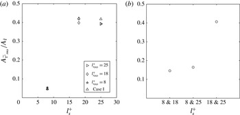
, the data collapse onto a single curve, which converges towards a value that agrees well with the amplitude of the turbulent oscillating wall shear stress plotted in figure 13(a).
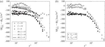
The time lag of the modulation of the axial and tangential turbulent fluctuations relative to the modulation of the centreline velocity in case I is plotted in figure 11(a). For
 $l_{s}^{+}=18$
and
 $l_{s}^{+}=25$
, there is a region
 $50<y^{+}<200$
where the modulations of both components of the turbulent fluctuations diffuse at similar rates,
 $|\text{d}y^{+}/\text{d}{\rm\Delta}t^{+}|\approx 0.4$
, in agreement with the data of Tardu et al. (Reference Tardu, Binder and Blackwelder1994) and Scotti & Piomelli (Reference Scotti and Piomelli2001) for large
 $l_{s}^{+}$
. Consequently, for pulsations of sufficiently low frequency (
 $l_{s}^{+}>15$
, say), there is a region in which the diffusivity of the modulation of the turbulent kinetic energy,
 ${\it\nu}_{\tilde{k}}^{+}$
, is of order
 $0.4y^{+}$
. This value is similar to the diffusivity of the turbulent kinetic energy in the overlap region of high-Reynolds-number steady pipe and channel flows, which scales with
 ${\it\kappa}y^{+}$
(see Pope Reference Pope2000).
In the near-wall region for
 $y^{+}\lesssim 50$
, the time lag of the modulation of the tangential velocity fluctuations relative to the modulation of the axial centreline velocity remain nearly constant regardless of the forcing frequency (even though the constant value differs between the pulsations). A plausible explanation for the constancy of the phase of
 $\widetilde{w^{\prime }w^{\prime }}$
in this region lies in the mechanism by which energy is supplied to this component. For
 $y^{+}<50$
, the main source term for
 $\widetilde{w^{\prime }w^{\prime }}$
is through redistribution by pressure strain from the modulation of the axial turbulent fluctuations. The finite time scale involved in this process causes the constant time lag of
 $\widetilde{w^{\prime }w^{\prime }}$
. Further out in the flow (
 $y^{+}>60$
), where turbulence diffusion becomes important in the energy budget, the modulation of the velocity fluctuations of both the tangential and axial components diffuse into the core at similar rates. Thus, as the core is approached, the time scale of the redistribution by pressure strain becomes negligible compared to that of the turbulence diffusion. The responses of
 $\widetilde{u^{\prime }u^{\prime }}$
and
 $\widetilde{w^{\prime }w^{\prime }}$
resemble those found for
 $\overline{u^{\prime 2}}$
and
 $\overline{w^{\prime 2}}$
in the study of transient accelerating pipe flow by He & Jackson (Reference He and Jackson2000). They showed that turbulence initially responds to the imposed acceleration by an increase of
 $\overline{u^{\prime 2}}$
in the buffer layer, whereas the time delay of
 $\overline{w^{\prime 2}}$
relative to the imposed acceleration is independent of position up to
 $y^{+}=50$
. Beyond this point, both components were shown to diffuse into the core at similar speeds.
Amplitude of the oscillating wall shear stress normalized by the Stokes amplitude. (a) Case I and individual harmonics from case II. (b) Case II non-decomposed. SP, data from Scotti & Piomelli (Reference Scotti and Piomelli2001); TBB, data from Tardu et al. (Reference Tardu, Binder and Blackwelder1994).

The time lag of the individual modes in case II was calculated from the respective Fourier series. The profiles for
 $l_{s_{IND}}^{+}=25$
and
 $l_{s_{IND}}^{+}=18$
, taken from the combination
 $l_{s}^{+}=25$
and 18, are plotted on figure 11(b). The difference from case I is small, and the same is true for the individual modes at the other combinations of pulsations as well. These data have, however, been left out from the figure.
3.2.3. Amplitude of the oscillating wall shear stress
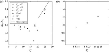
Considering case I plotted on figure 12(a), the amplitude of the oscillating wall shear stress normalized with the laminar Stokes value
 $A_{\widetilde{{\it\tau}}_{s}}=\sqrt{2}A_{\widetilde{U}_{c}}{\it\mu}/l_{s}$
displays features that are similar to those of the amplitude of the oscillating velocity plotted in figure 7(a). At the highest investigated frequency,
 $l_{s}^{+}=8$
, the normalized amplitude is approximately 95 % of the laminar value, which indicates that the effect of the shear wave generated at the wall is mainly confined within the viscous sublayer in which the turbulence is negligible. As a result, the oscillating velocity gradient is not appreciably different from that in a laminar flow, which results in an amplitude of the wall shear stress that is similar to that in the Stokes solution.
For
 $l_{s}^{+}=18$
, the amplitude of the oscillating wall shear is close to that of the laminar value, even though the velocity measurements at this frequency have displayed characteristics of a turbulent flow. Several previous studies (Ronneberger & Ahrens Reference Ronneberger and Ahrens1977; Mao & Hanratty Reference Mao and Hanratty1986; Tardu et al.
Reference Tardu, Binder and Blackwelder1994; Scotti & Piomelli Reference Scotti and Piomelli2001) have identified a minimum of
 $A_{\widetilde{{\it\tau}}}$
in the neighbourhood of
 $l_{s}^{+}=14$
. This effect was first noted by Ronneberger & Ahrens (Reference Ronneberger and Ahrens1977), who observed a minimum of
 $A_{\widetilde{{\it\tau}}}$
for
 $l_{s}^{+}\approx 11$
. They predicted this minimum by modelling turbulence as a rigid wall located outside the viscous sublayer at
 $y^{+}=15$
. For
 $l_{s}^{+}$
of
 $O(10{-}15)$
, the wavelength of the shear wave generated at the wall matches the distance to the ‘turbulent wall’. Destructive interference between the wave generated at the wall and the reflected wave was used to explain the minimum. The model showed qualitative agreement with their experimental data. However, because the LDV measurements presented in figure 7(a) follow the Stokes solution as long as
 $y_{s}<1$
, another potential explanation for the low value of the oscillating wall shear stress is due to an effective viscosity,
 ${\it\nu}_{e}$
. The similarity between the measured profile and the Stokes solution suggests that, close to the wall, a modified version of the laminar equation holds, i.e.
 $$\begin{eqnarray}\frac{\partial \widetilde{U}}{\partial t}=-\frac{1}{{\it\rho}}\frac{\partial \widetilde{p}}{\partial x}+\frac{1}{r}\frac{\partial }{\partial r}\left(r{\it\nu}_{e}\frac{\partial \widetilde{U}}{\partial r}\right),\end{eqnarray}$$
where the effects of the turbulence have been captured in the effective viscosity,
 ${\it\nu}_{e}$
, being the sum of the molecular and eddy viscosities. Equation (3.3) has solutions similar to (3.2), and thus the amplitude of the oscillating wall shear stress is approximately given by
 $A_{\widetilde{{\it\tau}}}\approx \sqrt{2}A_{\widetilde{U}_{c}}{\it\mu}/l_{s_{e}}$
, where
 $l_{s_{e}}=\sqrt{2{\it\nu}_{e}/{\it\omega}}$
is the effective Stokes length. Because
 $l_{s_{e}}$
grows with the square root of
 ${\it\nu}_{e}$
, the amplitude of the oscillating wall shear stress for
 $l_{s}^{+}=18$
is smaller than the purely viscous value
 $A_{\widetilde{{\it\tau}}_{s}}=\sqrt{2}A_{\widetilde{U}_{c}}{\it\mu}/l_{s}$
.
In the low-frequency regime, the flow tends towards a quasi-equilibrium in which the oscillating components of the centreline velocity and the wall shear stress are nearly in phase. From a phase-averaged version of the Blasius friction relation, Tardu et al. (Reference Tardu, Binder and Blackwelder1994) derived an estimate for the relative amplitude of the oscillating wall shear stress
 $A_{\widetilde{{\it\tau}}_{qs}}/A_{\widetilde{{\it\tau}}_{s}}=0.058l_{s}^{+}$
. For
 $l_{s}^{+}=25$
, the normalized amplitude becomes 1.45, thus being in good agreement with the measured wall shear stress, which overshoots the viscous Stokes value by 40 %. One reason for the small discrepancy might be that an
 $l_{s}^{+}$
value of 25 is too low to be considered quasi-steady, the exact limit being subtle to determine precisely. The data from Tardu et al. (Reference Tardu, Binder and Blackwelder1994) and Scotti & Piomelli (Reference Scotti and Piomelli2001) have been included in figure 12(a) for comparison – the results are in fairly good agreement.
The amplitude of the oscillating wall shear stress in case II,
 $A_{\widetilde{{\it\tau}}}=(\max (\widetilde{{\it\tau}})-\min (\widetilde{{\it\tau}}))/2$
, is plotted on figure 12(b). The data have been normalized with the viscous Stokes amplitude, which is defined as
 $A_{\widetilde{{\it\tau}}_{s}}=(\max (\widetilde{{\it\tau}}_{s})-\min (\widetilde{{\it\tau}}_{s}))/2$
, where
 $\widetilde{{\it\tau}}_{s}$
is approximately given by
 $\widetilde{{\it\tau}}_{s}\approx \sum \sqrt{2}A_{\widetilde{U}_{c_{n}}}{\it\mu}\cos ({\it\omega}_{n}t-{\rm\pi}/4)/l_{s_{n}}$
. When one pulsation is at
 $l_{s}^{+}=8$
, the deviations from the Stokes solutions are approximately
 $\pm$
5 %, in line with the LDV measurements, which follow the Stokes solutions quite closely for
 $y_{s}<0.6$
. For the combination
 $l_{s}^{+}=25$
and 18, the oscillating wall shear stress amplitude overshoots the laminar value by 20 %, which also conforms with the LDV measurements, which are larger than the Stokes value for
 $y_{s}<0.4$
. Because of the relatively long period time of both oscillations for this combination of frequencies, the amplitude of the oscillatory wall shear stress can be estimated from the Blasius relation by assuming quasi-steady flow. Then, at any instant of the oscillating cycle, the phase-averaged wall shear stress is given by
 $$\begin{eqnarray}\langle {\it\tau}_{qs}\rangle =\frac{1}{8}{\it\rho}\langle U_{c}\rangle ^{2}K\left(\frac{\langle U_{c}\rangle D}{{\it\nu}}\right)^{-1/4},\end{eqnarray}$$
where
 $K$
is a constant and
 $\langle U_{c}\rangle =\overline{U}_{c}+\widetilde{U}_{c}$
. Expanding (3.4) around
 $\overline{U}_{c}$
and keeping terms up to linear order yields
 $$\begin{eqnarray}\widetilde{{\it\tau}}_{qs}=\frac{7}{4}\bar{{\it\tau}}\frac{\widetilde{U}_{c}}{\overline{U}_{c}}\end{eqnarray}$$
for the periodic component. Taking
 $\widetilde{U}_{c}=A_{\widetilde{U}_{c_{1}}}\sin ({\it\omega}t)+A_{\widetilde{U}_{c_{2}}}\sin (2{\it\omega}t)$
as the oscillatory part of the velocity and simplifying the analysis by assuming that
 $A_{\widetilde{U}_{c_{1}}}=A_{\widetilde{U}_{c_{2}}}$
, being true to within 5 % in the current measurements, it follows that
 $$\begin{eqnarray}\frac{A_{\widetilde{{\it\tau}}_{qs}}}{A_{\widetilde{{\it\tau}}_{s}}}=0.058l_{s}^{+}\frac{A[\sin ({\it\omega}t)+\sin (2{\it\omega}t)]}{A[\cos ({\it\omega}t-{\rm\pi}/4)+\sqrt{2}\cos (2{\it\omega}t-{\rm\pi}/4)]}\approx 1.21,\end{eqnarray}$$
where
 $A[\cdots ]$
is the amplitude of the argument and the factor 0.058 results from
 $\bar{u}_{{\it\tau}}/\overline{U}_{c}\approx 0.048$
. The measured value corresponds well with the theoretical prediction, although only one pulsation is of low enough frequency to approach the limit of quasi-steadiness. A similar analysis was applied to the combination
 $l_{s}^{+}=25$
and 8 but without successful correlation because of the high frequency of the
 $l_{s}^{+}=8$
pulsation.
Amplitude of the oscillating wall shear stress turbulent fluctuations normalized by the oscillating wall shear stress. (a) Case I and individual harmonics from case II. (b) Case II non-decomposed.

The amplitudes of the individual modes of the phase-averaged wall shear stress in case II, normalized with the corresponding Stokes values, are also plotted on figure 12(a). The results from case I serve as reference data, and, as can be seen from the figure, the amplitude of the individual modes are all within
 $\pm$
5 % of the reference.
3.2.4. Amplitude of the oscillating turbulent wall shear stress
As shown in §§ 3.2.1 and 3.2.2, the oscillating velocity in case I undergoes a transition from a turbulent regime to a quasi-laminar regime in the range of
 $10<l_{s}^{+}<15$
. Over this range of
 $l_{s}^{+}$
, the turbulence intensity decreases significantly and the oscillating velocity no longer admits a logarithmic distribution. The turbulent to laminar transition is clearly manifested in the oscillating component of the r.m.s. turbulent fluctuating wall shear stress plotted on figure 13(a) as well. The amplitude is eight times smaller for
 $l_{s}^{+}=8$
than at the other two frequencies and in close agreement with the LDV measurements. The amplitudes at
 $l_{s}^{+}=18$
and
 $l_{s}^{+}=25$
are similar, which conforms with the collapse of the turbulence intensity profiles observed in the LDV measurements plotted in figure 10(e). The individual harmonics from case II have been included with the case I data in figure 13(a). The harmonics from case II are within
 $\pm$
5 % of the values from case I, thereby conforming with the previous data showing negligible interactions between the pulsations. The full response of the case II measurement data plotted in figure 13(b) is also in line with the velocity measurements. When one pulsation is at
 $l_{s}^{+}=8$
, the turbulence intensities collapse to the same value, and, at the combination
 $l_{s}^{+}=25$
and 18, the turbulence intensity takes the same value as when these pulsations are imposed alone.
4. Conclusions
Velocity and turbulence profiles acquired with LDV and hot-film wall shear stress measurements in a turbulent pulsating pipe flow have been presented. Measurements have been performed at three pulsation frequencies,
 ${\it\omega}^{+}=0.003$
, 0.006 and 0.03, ranging from the low-frequency regime to the quasi-laminar regime. The present study extends previous work in pulsating flows in that it covers the simultaneous imposition of two pulsations (case II) in addition to the single-frequency case (case I). The case II measurements were produced by combining the aforementioned pulsations two at a time, yielding a total of seven sets of data, including steady-state measurements. The measurements from case I were presented first to serve as a reference for the data from case II. The most notable finding of this study is that interactions between the pulsations in case II are negligible, i.e. the oscillating component of each flow quantity is simply the superposition of the corresponding quantities from case I.
The time-averaged quantities are largely unaffected by the unsteadiness, which corresponds with the previously established view that the mean flow is decoupled from the oscillatory flow. The Stokes length scaled in wall units
 $l_{s}^{+}=\sqrt{2/{\it\omega}^{+}}$
has been shown to be the appropriate similarity parameter for correlating the near-wall data. In the range
 $10<l_{s}^{+}<15$
, the oscillatory flow undergoes a transition from a quasi-laminar regime to a turbulent regime. In the turbulent regime, the oscillatory velocity exhibits features similar to its time-averaged counterpart, displaying a logarithmic velocity distribution in a region in which the direct effect of the molecular viscosity and the centreline is small. Additionally, the turbulence intensities collapse onto a single curve. When the flow is in the quasi-laminar regime, both the oscillating velocity and wall shear stress tend towards the purely viscous Stokes solution and the amplitude of the modulation of turbulence is small. At the lowest investigated frequency in cases I and II, asymptotic quasi-steady analyses predict the amplitude of the oscillating wall shear stress fairly well.
Acknowledgements
The research presented was carried out as a part of ‘Swedish Hydropower Centre – SVC’. SVC has been established by the Swedish Energy Agency, Elforsk and Svenska Kraftnät together with Luleå University of Technology, The Royal Institute of Technology, Chalmers University of Technology and Uppsala University (see http://www.svc.nu).