1. Introduction
Many underwater animals have evolved propulsive strategies to travel with minimal energy expenditure. They adapt their strategies to unsteady flows prevalent in underwater habitats, allowing them to harness energy from their surroundings and minimise the energy expenditure for propulsion (Liao Reference Liao2007). A free surface with waves is a typical aquatic environment that induces unsteady flows beneath it (Airy Reference Airy1845). In such environments, animals such as dolphins, sea lions and certain fish species employ specific strategies such as wave riding or surface skimming to interact with wave-driven flows, effectively harnessing wave energy for propulsion (Fish Reference Fish1993; Williams, Friedl & Haun Reference Williams, Friedl and Haun1993; Weihs Reference Weihs2002; Fish & Lauder Reference Fish and Lauder2006).
Inspired by these natural adaptations, many theoretical, numerical and experimental studies have explored the propulsion of foils oscillating under a free surface with and without incident waves. In a theoretical study, Grue, Mo & Palm (Reference Grue, Mo and Palm1988) demonstrated that the thrust of a foil decreases when plunging near a free surface; however, when plunging and pitching motions are combined, the thrust remains similar to that far from the surface. A hydrofoil undergoing plunging motion was also investigated in an experimental study by Cleaver (Reference Cleaver, Calderon, Wang and Gursul2013) and a numerical study by Esmaeilifar et al. (Reference Esmaeilifar, Djavareshkian, Feshalami and Esmaeili2017); both reported increased drag near a free surface. Esmaeilifar et al. (Reference Esmaeilifar, Djavareshkian, Feshalami and Esmaeili2017) found that a trailing-edge vortex was induced as the foil approached the free surface, thereby increasing the drag on the foil. Zhu, Liu & Yue (Reference Zhu, Liu and Yue2006) and Filippas & Belibassakis (Reference Filippas and Belibassakis2014) employed a boundary-element method to simulate the motion of a flapping foil near a free surface. Consistent with other studies, they reported that proximity to the free surface negatively influences thrust due to the resistance caused by flapping-motion-induced waves at the free surface. However, a foil oscillating at a low frequency could result in increased thrust and efficiency (Zhu et al. Reference Zhu, Liu and Yue2006). Recently, Zheng et al. (Reference Zheng, He, Zhao, Shen and Zhu2024) discovered an optimal Froude number range in their numerical study, where a rigid plate flapping under a free surface without incident waves exhibited improved efficiency.
As reviewed above, rigid foil flapping under a free surface generally results in reduced propulsive performance (for more discussion, see Filippas & Belibassakis Reference Filippas and Belibassakis2014; Chung Reference Chung2016; Esmaeilifar et al. Reference Esmaeilifar, Djavareshkian, Feshalami and Esmaeili2017; Deng et al. Reference Deng, Wang, Kandel and Teng2022; Lopes et al. Reference Lopes, Vaz, De Campos and Sarmento2023), except within an optimal range of the unsteady parameter (Zhu et al. Reference Zhu, Liu and Yue2006) or the Froude number (Zheng et al. Reference Zheng, He, Zhao, Shen and Zhu2024), where enhanced performance has been reported. In the presence of an incident surface wave, however, the hydrodynamic advantages of an oscillating foil have been observed in both theoretical (Wu Reference Wu1961, Reference Wu1972; Isshiki Reference Isshiki1982; Grue et al. Reference Grue, Mo and Palm1988) and numerical (De Silva & Yamaguchi Reference De Silva and Yamaguchi2012; Filippas & Belibassakis Reference Filippas and Belibassakis2014; Liu et al. Reference Liu, Liu, Huang, Zhao and Su2018; Wang et al. Reference Wang, Li, Yan and Zhang2022; Zhu et al. Reference Zhu, Tai, Du and Zhang2022) studies. Energy extraction by a foil is feasible when the incoming flow contains a wave component because it induces a transverse flow normal to the foil span (Wu Reference Wu1961, Reference Wu1972). Isshiki (Reference Isshiki1982) incorporated the free-surface effect into Wu’s theory and suggested the use of wave energy for ship propulsion, known as wave-devouring propulsion. Grue et al. (Reference Grue, Mo and Palm1988) reached a similar conclusion that a portion of wave energy can be extracted through the oscillatory motion of a foil in incoming waves. The amount of energy extraction largely depends on the phase difference between the wave motion and the foil motion. A rigid foil flapping under the wave surface achieves maximum efficiency and thrust when the heaving motion of the foil has a
 $\pi /2$
phase difference from the wave (De Silva & Yamaguchi Reference De Silva and Yamaguchi2012; Filippas & Belibassakis Reference Filippas and Belibassakis2014; Liu et al. Reference Liu, Liu, Huang, Zhao and Su2018).
Previous research on the effects of waves on the propulsive performance of actively flapping foils, as reviewed above, focused on rigid bodies as propulsors (De Silva & Yamaguchi Reference De Silva and Yamaguchi2012; Filippas & Belibassakis Reference Filippas and Belibassakis2014,Reference Filippas and Belibassakis2022; Zhu et al. Reference Zhu, Tai, Du and Zhang2022). However, most biological propulsors in nature are flexible, facilitating energy extraction from their ambient fluid environments (Liao et al. Reference Liao, Beal, Lauder and Triantafyllou2003; Liao Reference Liao2007; Park, Kim & Sung Reference Park, Kim and Sung2016; Park & Sung Reference Park and Sung2016,Reference Park and Sung2018). Liu et al. (Reference Liu, Liu, Huang, Zhao and Su2018) prescribed the deformation of a foil oscillating under a wave to partially reflect its flexible characteristics. They reported that the deformed foil obtained improved propulsive performance and energy recovery from an incident wave. However, owing to its prescribed deformation, the dynamic interaction between the foil and the surrounding fluid was not considered. The flapping kinematics, which are dynamically governed by the two-way interaction between the fluid and the flexible body, might be an essential factor that determines the propulsive performance of a flexible foil near a wave surface. To our knowledge, except for the work of Li et al. (2025), where a passive flexible foil with a fixed leading edge (in contrast to the present study where the foil’s leading edge actively heaves) was investigated, few studies have explored the hydrodynamics of a flexible foil near a free surface in the presence of an incident wave.
The present study examines the hydrodynamics of an actively heaving flexible foil under a wave surface. Unlike previous studies that considered rigid foils or foils with prescribed deformations (De Silva & Yamaguchi Reference De Silva and Yamaguchi2012; Filippas & Belibassakis Reference Filippas and Belibassakis2014; Liu et al. Reference Liu, Liu, Huang, Zhao and Su2018; Zhu et al. Reference Zhu, Tai, Du and Zhang2022), this research fully considers the flexible characteristics of a foil by solving a nonlinear elastic motion equation, which dynamically determines its flapping kinematics in the presence of water waves. Because an incident wave induces a sinusoidal horizontal and vertical flow varying with time and space, it significantly affects the kinematics and dynamics of a flexible foil and, consequently, its propulsive performance.
The remainder of this paper is organised as follows. Section 2 introduces an immersed-boundary (IB) method to simulate the interaction between a flexible foil and the surrounding fluid. It also introduces a coupled level set and volume-of-fluid (CLSVOF) method to capture the air–water interface. After describing the problem formulation and numerical method in
 $\S$
2,
 $\S$
3 presents the results and discussion. The simulation parameters are described in
 $\S$
3.1. In
 $\S$
3.2, we present the results on the effects of the submergence depth and the ratio of the foil’s heaving frequency to that of the incident wave, where we investigate the vortical structures produced by the foil near the wave surface to elucidate the underlying mechanism contributing to either the enhancement or reduction in propulsive performance. Next, we analyse the effects of the phase difference between the foil’s heaving motion and the incident wave in
 $\S$
3.3, followed by a scaling analysis to quantify the relation between the foil’s kinematics and propulsive performance in
 $\S$
3.4. Finally, the conclusions are presented in
 $\S$
4.
2. Problem formulation and numerical method
Direct numerical simulation is performed to study the hydrodynamics of a flexible foil in a wave field superposed with a uniform current with a velocity of
 $u_\infty$
. In this study, we consider two dimensions. We also neglect the effect of the foil thickness on the flow. Figure 1 shows the computational domain, schematics of the boundary conditions and the flexible foil under the wave. As shown in figure 1(a), Dirichlet boundary conditions are imposed on the inlet, top and bottom boundaries of the computational domain. The convective boundary condition is applied at the outlet boundary. To artificially dissipate surface waves and prevent wave reflection, a sponge layer is introduced near the outlet. For subcritical conditions, the waves can propagate both upstream and downstream. In the present cases, we did not observe upstream-propagating waves. Therefore, no additional treatment for suppressing wave reflection was needed in our study. But we caution that it might be necessary in other scenarios. Figure 1(b) shows a schematic diagram of a flexible foil with a length of
 $L$
, where its leading edge is positioned at an average depth
 $D$
below the mean free surface. A sinusoidal heaving motion with amplitude
 $A_{\!f}$
is imposed on the leading edge, whereas the posterior parts of the foil oscillate passively because of the fluid–flexible structure interaction.
In our simulation, the motion of the flexible foil is described via a moving Lagrangian grid system defined on the foil and governed by a nonlinear elastic motion equation. The fluid motion is described on a fixed Eulerian grid and is governed by the Navier–Stokes equations. We employ the IB method to simulate the interaction between the fluid and flexible foil motions (Huang, Shin & Sung Reference Huang, Shin and Sung2007; Park & Sung Reference Park and Sung2018; He et al. Reference He, Yang, Sotiropoulos and Shen2022b ). The wave motion is simulated via the CLSVOF method to capture the air–water interface. The CLSVOF method combines the strengths of accurate interface geometry representation of the level set (LS) method and the precise mass conservation for each fluid of the volume-of-fluid (VOF) method (Sussman & Puckett Reference Sussman and Puckett2000). The details of the various aspects of the numerical schemes and their validations are provided in our previous publications (e.g. Yang et al. Reference Yang, Lu, Guo, Liu and Shen2017; Cui et al. Reference Cui, Yang, Jiang, Huang and Shen2017; Yang, Deng & Shen Reference Yang, Deng and Shen2018; He, Liu & Shen Reference He, Liu and Shen2022a ) and are not repeated here. Their key features are introduced in the following subsections.
(a) Computational domain and boundary conditions. (b) Schematic diagram of a flexible foil (illustrated in red) flapping under a surface wave. The incident wave has a wave amplitude
 $A_w$
and frequency
 $f_w$
. The surface elevation above the foil’s leading edge is from the wave boundary condition and is denoted by
 $\eta _l$
. The heaving motion of the foil is described by the heaving amplitude
 $A_{\!f}$
, frequency
 $f_{\!f}$
and phase difference
 $\mathit \varPhi$
, which lags the surface elevation oscillation. The convective velocity in the outflow boundary condition is denoted by
 $c$
.

2.1. Governing equations for fluid motion and their numerical solver
The water and air motions are governed by the Navier–Stokes equations for Newtonian, incompressible flows:
 \begin{align} \frac {\partial \boldsymbol{\mathit{u}}}{\partial t} + \boldsymbol{\mathit{u}} \boldsymbol{\cdot }\boldsymbol{\nabla }\boldsymbol{\mathit{u}} = \frac {1}{\rho (\phi )} &\left [-\boldsymbol{\nabla }p + \boldsymbol{\nabla }\boldsymbol{\cdot }(\mu (\phi ) \boldsymbol{\mathit{S}}) + \rho (\phi ) \boldsymbol{\mathit{g}} \right ] + \boldsymbol{\mathit{f}}, \end{align}
 \begin{align}&\,\, \boldsymbol{\nabla }\boldsymbol{\cdot }\boldsymbol{\mathit{u}}= 0, \end{align}
where
 $\boldsymbol{\mathit{u}}$
is the fluid velocity,
 $\rho$
is the phase-dependent (water or air) density,
 $\phi$
is the LS function,
 $p$
is the pressure,
 $\mu$
is the phase-dependent (water or air) dynamic viscosity,
 $\boldsymbol{\mathit{S}} = (\boldsymbol{\nabla }\boldsymbol{\mathit{u}} + \boldsymbol{\nabla }\boldsymbol{\mathit{u}}^{\mathrm{\mathit{T}}}) / 2$
is the strain rate tensor,
 $\boldsymbol{\mathit{g}}$
is the gravitational acceleration and
 $\boldsymbol{\mathit{f}}$
is the force exerted by the flexible foil. The LS function
 $\phi (\boldsymbol{\mathit{x}})$
is a signed function denoting the distance between point
 $\boldsymbol{\mathit{x}}$
and the nearest point
 $\boldsymbol{\mathit{x_s}}$
on the air–water interface and is defined as
 \begin{equation} \phi (\boldsymbol{\mathit{x}}) = \begin{cases} -|\boldsymbol{\mathit{x}} - \boldsymbol{\mathit{x_s}}|, & \quad \text{for } \boldsymbol{\mathit{x}} \text{ in water,} \\ \quad 0, & \quad \text{for } \boldsymbol{\mathit{x}} \text{ at the interface,} \\ |\boldsymbol{\mathit{x}} - \boldsymbol{\mathit{x_s}}|, & \quad \text{for } \boldsymbol{\mathit{x}} \text{ in air.} \end{cases} \end{equation}
The fluid density
 $\rho$
and fluid viscosity
 $\mu$
are phase-dependent and defined as
 \begin{equation} \begin{aligned} \rho (\phi ) &= \rho _a H_{\mathit{\varepsilon }}(\phi ) + \rho _w \big (1 - H_{\mathit{\varepsilon }}(\phi )\big ), \\ \mu (\phi ) &= \mu _a H_{\mathit{\varepsilon }}(\phi ) + \mu _w \big (1 - H_{\mathit{\varepsilon }}(\phi )\big ), \end{aligned} \end{equation}
where the subscripts ‘
 $ a$
’ and ‘
 $ w$
’ denote air and water, respectively. The density ratio
 $ \rho _a / \rho _w$
is 0.0012 and the viscosity ratio
 $ \mu _a / \mu _w$
is 0.0182. The smoothed Heaviside function,
 $H$
in (2.4), is defined by
 \begin{equation} H_\varepsilon (\phi ) = \begin{cases} 0, & \phi \lt -\varepsilon \\[6pt] \dfrac {1}{2} \left [ 1 + \dfrac {\phi }{\varepsilon } + \dfrac {1}{\pi } \sin \left ( \dfrac {\phi \pi }{\varepsilon } \right ) \right ], & -\varepsilon \leqslant \phi \leqslant \varepsilon \\[6pt] 1, & \phi \gt \varepsilon , \end{cases} \end{equation}
where
 $\varepsilon$
is three times the length of the smallest grid cell near the air–water interface (Osher & Fedkiw Reference Osher and Fedkiw2006).
The air–water interface is captured by the CLSVOF method, in which both the LS function
 $\phi$
and the VOF function
 $\mathit{F}$
are updated at each computational time step by solving the following convection equations:
 \begin{equation} \begin{aligned} \frac {\partial \phi }{\partial t} + \boldsymbol{\nabla }\boldsymbol{\cdot }(\boldsymbol{\mathit{u}} \phi ) = 0,\\ \frac {\partial F}{\partial t} + \boldsymbol{\nabla }\boldsymbol{\cdot }(\boldsymbol{\mathit{u}} F) = 0. \end{aligned} \end{equation}
The incident wave is prescribed at the inlet boundary. In the case of deep-water waves satisfying
 $h \gt {\lambda }/{2}$
, where
 $h$
is the water depth and
 $\lambda$
is the wavelength, the horizontal and vertical orbital velocities for small-amplitude waves superimposed with the uniform velocity
 $u_\infty$
are
 \begin{equation} \begin{aligned} u_{in,x}(x, y, t) &= u_\infty +\sigma A_w {\rm e}^{-kD} \cos \theta _w,\\ v_{in,y}(x, y, t) &= \sigma A_w {\rm e}^{-kD} \sin \theta _w. \end{aligned} \end{equation}
In the above equations,
 $\sigma = \sqrt {gk}$
is the intrinsic angular frequency,
 $k$
is the wavenumber,
 $\theta _w$
is the wave phase determined by the position
 $x$
and time
 $t$
,
 $\theta _w = kx - \omega t$
, and
 $\omega$
is the observed angular frequency,
 $\omega = 2\pi f_w = \sqrt {gk} + k u_\infty$
. In the present study, the non-dimensional intrinsic angular frequency and the wavenumber are 2.48 and 0.628, which are normalised by
 $u_\infty / L$
and
 $1 / L$
, respectively. The wavelength is
 $\lambda = 10L$
and the water depth is
 $h = 8L$
, satisfying the deep-water wave condition, i.e.
 ${\lambda }/{2} \lt h$
. The inlet position is
 $x = 0$
(figure 1).
2.2. Governing equations for flexible foil motion
The flexible foil is modelled as an inextensible nonlinear Euler–Bernoulli beam. The governing equation for the flapping motion of the flexible foil and its inextensibility condition are given by
 \begin{align} \rho _d \frac {\partial ^2 \boldsymbol{X}}{\partial t^2} = \frac {\partial }{\partial s} \left ( T \frac {\partial \boldsymbol{X}}{\partial s} \right ) &- \frac {\partial ^2}{\partial s^2} \left ( \gamma \frac {\partial ^2 \boldsymbol{X}}{\partial s^2} \right ) + \rho _d \boldsymbol{\mathit{g}} + \boldsymbol{\mathit{F}}, \end{align}
 \begin{align} \frac {\partial \boldsymbol{X}}{\partial s} &\boldsymbol{\cdot }\frac {\partial \boldsymbol{X}}{\partial s} = 1, \end{align}
respectively. In the above equations,
 ${\mathit{\rho }}_d$
is the density difference between the foil (
 ${\mathit{\rho }}_s$
) and the water (
 ${\mathit{\rho }}_w$
),
 $\boldsymbol{X}=(X(s,t),Y(s,t))$
is the Lagrangian position vector of the flexible foil,
 $s$
is the curvilinear Lagrangian coordinate along the foil,
 $T$
is the tension force applied along the foil,
 $\gamma$
is the bending stiffness per cross-sectional area of the foil and
 $\boldsymbol{F}$
is the Lagrangian momentum force caused by the interaction between the flexible structure and the fluid. The bending stiffness per cross-sectional area
 $\gamma$
is defined as
 ${E d^2}/{12}$
, where
 $E$
represents Young’s modulus and
 $d$
is the foil thickness set to be
 $1/100$
of the foil length
 $L$
. Since the foil is very thin, its thickness is considered to have a negligible effect on the flow.
The tension force is determined from the inextensibility constraint and is calculated by solving a Poisson equation derived from (2.8) and (2.9):
 \begin{equation} \frac {\partial \boldsymbol{X}}{\partial s} \frac {\partial ^2}{\partial s^2} \left ( T \frac {\partial \boldsymbol{X}}{\partial s} \right ) = \frac {1}{2} \frac {\partial ^2}{\partial t^2} \left ( \frac {\partial \boldsymbol{X}}{\partial s} \frac {\partial \boldsymbol{X}}{\partial s} \right ) - \frac {\partial ^2 \boldsymbol{X}}{\partial t \partial s} \frac {\partial ^2 \boldsymbol{X}}{\partial t \partial s} + \frac {\partial \boldsymbol{X}}{\partial s} \frac {\partial }{\partial s} \left ( \frac {\partial ^2}{\partial s^2} \left ( \gamma \frac {\partial ^2 \boldsymbol{X}}{\partial s^2} \right ) + \boldsymbol{F}\right ). \end{equation}
At the leading edge, the boundary conditions are
 \begin{equation} \boldsymbol{X} = (X_0, Y_0 + A_{\!f} \sin (2\pi f_{\!f} t + \mathit{\varPhi })), \quad \frac {\partial \boldsymbol{X}}{\partial s} = (1, 0) \quad \text{at } s = 0. \end{equation}
At the trailing edge, the boundary conditions are
 \begin{equation} T = 0, \quad \frac {\partial ^2 \boldsymbol{X}}{\partial s^2} = (0, 0), \quad \frac {\partial ^3 \boldsymbol{X}}{\partial s^3} = (0, 0) \quad \text{at } s = 1. \end{equation}
In (2.11), (
 $X_0$
,
 $Y_0$
) indicates the initial position of the leading edge,
 $f_{\!f}$
is the heaving frequency and
 $\mathit{\varPhi }$
is the phase difference between the vertical flow motion induced by the incident wave and the heaving motion of the leading edge. The boundary conditions (2.11) are applied to the leading edge, encompassing a combination of transverse harmonic heaving motion, a clamped condition and a horizontal constraint condition. Moreover, the free-end boundary conditions specified in (2.12) are imposed at the trailing edge.
2.3. Immersed-boundary method for fluid–foil interactions
The interaction force between the fluid and foil is calculated via the Eulerian momentum force
 $\boldsymbol{f}$
in (2.1) and the Lagrangian momentum force
 $\boldsymbol{F}$
in (2.10) on the basis of the feedback force law. Force
 $\boldsymbol{F}$
is determined from the following equation (Goldstein, Handler & Sirovich Reference Goldstein, Handler and Sirovich1993; Huang et al. Reference Huang, Shin and Sung2007):
 \begin{equation} \boldsymbol{F} = \alpha \int _0^t(\boldsymbol{U_{{ib}}}-\boldsymbol{U})\text{d}t+\beta (\boldsymbol{U_{{ib}}}-\boldsymbol{U}), \end{equation}
where
 $\alpha$
and
 $\beta$
are negative constants and
 $\boldsymbol{U}$
is the velocity of the foil expressed by
 $\boldsymbol{U} = \text{d}\boldsymbol{X} / \text{d}t$
. The constants in (2.13) are set to
 $\alpha = -10^{{-6}}$
and
 $\beta = -10^{{-3}}$
, and their dimensions are
 ${M}/{L}^3{T}^2$
and
 ${M}/{L}^3{T}$
, respectively (Huang et al. Reference Huang, Shin and Sung2007; He et al. Reference He, Liu and Shen2022a
, Reference He, Yang, Sotiropoulos and Shen2022b
). The subscript ‘
 $ib$
’ refers to the variables on the foil’s IB points, which move with the foil motion. Term
 $\boldsymbol{U}_{\!ib}$
is the fluid velocity interpolated on the IB, which is calculated by
 \begin{equation} \boldsymbol{U}_{\!ib}(s, t) = \int _\varOmega \boldsymbol{u}(\boldsymbol{\mathit{x}}, t) \delta (\boldsymbol{X}(s, t) - \boldsymbol{\mathit{x}}) \, \text{d}\boldsymbol{\mathit{x}}. \end{equation}
The position of the IB,
 $\boldsymbol{X}_{\!ib}$
, is expressed by
 \begin{equation} \boldsymbol{X}_{\!ib} = \boldsymbol{X}_{\!ib}^0 + \int _0^t \boldsymbol{U}_{\!ib} \, \text{d}t, \end{equation}
where
 $\boldsymbol{X}_{\!ib}^0$
is the initial position of the IB. The Dirac delta function
 $\delta ()$
in (2.14) allows for considering the interactions between a fluid, represented by Eulerian variables, and the flexible foil, represented by Lagrangian variables (Peskin Reference Peskin2002). The Eulerian momentum force is then calculated by spreading the Lagrangian force onto the nearby Eulerian grid:
 \begin{equation} \boldsymbol{f}(\boldsymbol{\mathit{x}}, t) = -\frac { d}{\rho _w} \int \boldsymbol{F}(s, t) \delta (\boldsymbol{\mathit{x}} - \boldsymbol{X}(s, t)) \text{d}s. \end{equation}
The combination of (2.13)–(2.16) indicates that the fluid at the surrounding Eulerian grid points moves with those at the Lagrangian grid points, thereby enforcing the no-slip boundary condition of the fluid on the foil.
The present solver has been used to simulate various air–water interaction and fluid–structure interaction problems in previous studies by our group (e.g. Cui et al. Reference Cui, Yang, Jiang, Huang and Shen2017; Yang et al. Reference Yang, Lu, Guo, Liu and Shen2017; Yang et al. Reference Yang, Deng and Shen2018; Kan et al. Reference Kan, Yang, Lyu, Zheng and Shen2021; He et al. Reference He, Liu and Shen2022a , Reference He, Yang, Sotiropoulos and Shen2022b ). For fluid–flexible structure interactions, He et al. (Reference He, Liu and Shen2022a ) reported that the results of a flapping foil in uniform flow agreed well with those of Huang et al. (Reference Huang, Shin and Sung2007) and Zhu, He & Zhang (Reference Zhu, He and Zhang2014). A flexible stem, with one end fixed on the bottom wall, was simulated under uniform flow by He et al. (Reference He, Yang, Sotiropoulos and Shen2022b ), and the hydrodynamic force applied to it agreed well with the results of Luhar & Nepf (Reference Luhar and Nepf2011). He et al. (Reference He, Yang, Sotiropoulos and Shen2022b ) also conducted a simulation of water impinging onto the free end of a rubber gate and compared the results with those reported by Antoci, Gallati & Sibilla (Reference Antoci, Gallati and Sibilla2007) and Jahanbakhsh et al. (Reference Jahanbakhsh, Vessaz, Maertens and Avellan2015), demonstrating good agreement. Because extensive tests have been reported in our previous papers cited above, they are not repeated in this paper to accommodate paper length.
3. Results and discussion
3.1. Simulation parameters
As introduced in
 $\S$
2, a two-dimensional flexible foil oscillating under the air–water interface of an incident wave superposed by a uniform flow (
 $u_\infty$
= 0.01 m s−1) is modelled. The properties of the flexible foil and the fluid (see figure 1) are as follows: foil length
 $L$
=
 $0.01$
m, foil density
 $\rho _s$
=
 $2.0$
 $\times$
 $10^3$
kg m−
 $^3$
, Young’s modulus of the flexible foil
 $E$
= 10
 $^6$
Pa (
 $\gamma$
= 8.33
 $\times$
10
 $^{-4}$
), air density
 $\rho _a$
= 1.2 kg m−
 $^3$
, air viscosity
 $\mu$
 $_a$
= 1.82
 $\times$
10
 $^{-5}$
Pa s, water density
 $\rho _w$
= 1000 kg m−
 $^3$
and water viscosity
 $\mu$
 $_w$
= 10
 $^{-3}$
Pa s. The density and Young’s modulus of the flexible foil are chosen to be similar to those typically found in small biological propulsors (Tytell et al. Reference Tytell, Hsu, Williams, Cohen and Fauci2010). By fixing the foil’s flexibility within a biologically relevant range, we focus more closely on investigating the fundamental dynamics of a flexible foil interacting with wave-induced flow, particularly examining the influence of its kinematics on the hydrodynamic propulsive performance in the following sections. The dimensionless parameters are listed in table 1. The length, velocity and time are normalised by the foil length
 $L$
, free-stream velocity
 $u_\infty$
and
 $L/u_\infty$
, respectively. The Reynolds number based on the water density, water viscosity, foil length and free-stream velocity is 100, i.e.
 $Re = \rho _w u_\infty L /\mu _w=100$
. According to Leis & Carson-Ewart (Reference Leis and Carson-Ewart1997) and Downie et al. (Reference Downie, Illing, Faria and Rummer2020), small fish with body lengths of approximately
 $ 10^{-2}$
m swim at about 1–2 body lengths per second. At this length scale, the Reynolds number is of the order of 100, similar to that used in our study. The flexible foil is discretised into 24 elements, and the fluid domain is discretised by 960 (
 $x$
)
 $\times$
480 (
 $y$
) grid points, which are clustered near the flexible foil and stretched in both the
 $x$
and
 $y$
directions. The origin of time is chosen such that the wave-surface elevation above the leading edge of the foil can be described as
 $\eta _l$
(
 $t$
) =
 $8L + A_w \cos (2\pi f_wt)$
, where 8
 $L$
is the mean water level and
 $A_w$
is the wave amplitude.
Parameters of the simulations. The length, velocity and time are normalised by the foil’s length
 $L$
, free-stream velocity
 $u_\infty$
and
 $L/u_\infty$
, respectively.

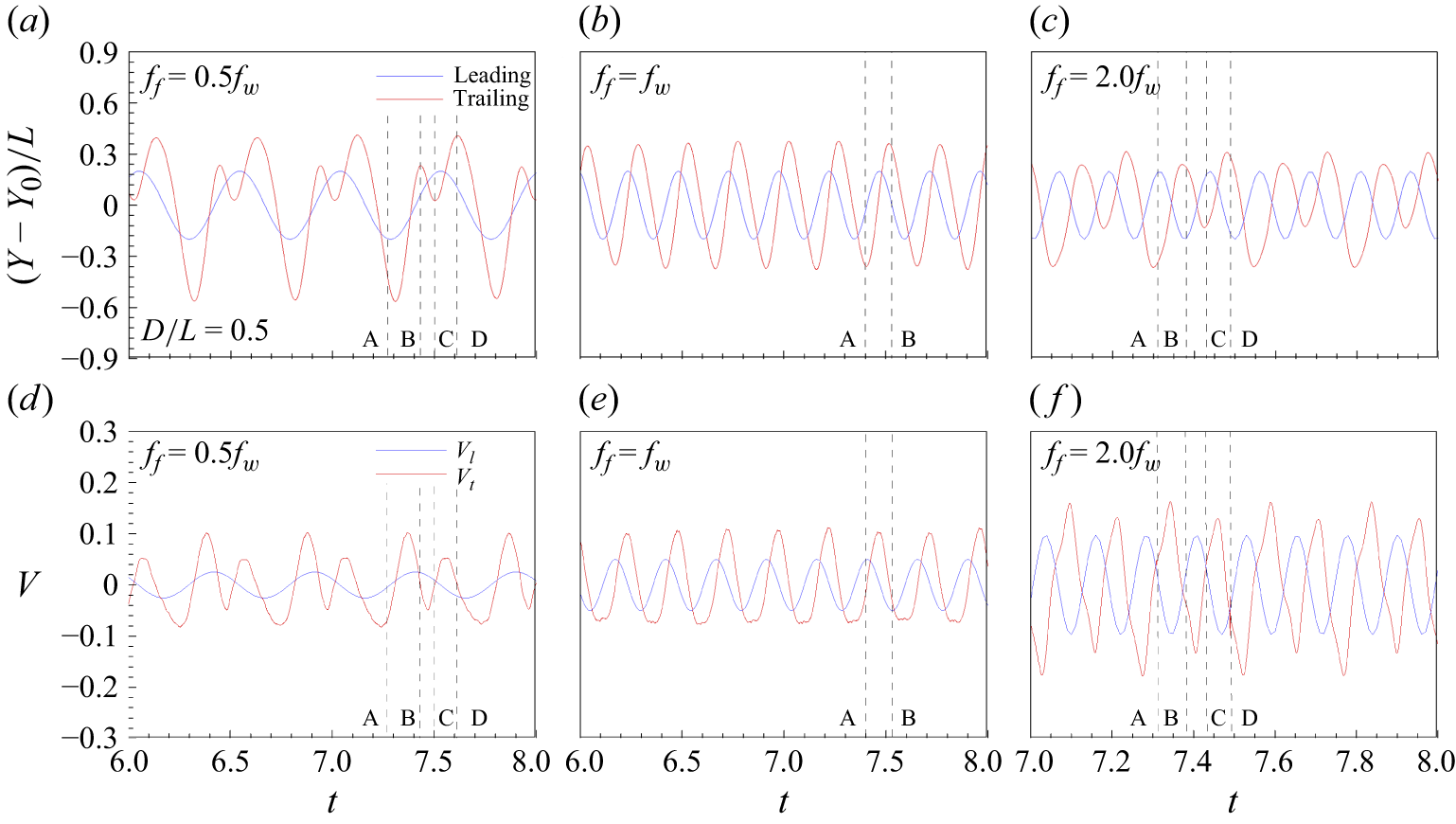
Histories of the leading- and trailing-edge (a–c)
 $y$
positions and (e–f) vertical velocities for different heaving frequencies: (a,d)
 $f_{\!f}$
 $=$
0.5
 $f_w$
, (b,e)
 $f_{\!f}$
 $=$
 $f_w$
and (c,f)
 $f_{\!f}$
 $=$
2.0
 $f_w$
. The blue and red solid lines denote the leading and trailing edges, respectively, and the black dashed lines represent the times corresponding to instants A–D. The mean submergence depth is
 $D/L = 0.5$
, and the phase difference between the heaving motion and incident wave is
 $\mathit{\varPhi }$
 $=$
0.

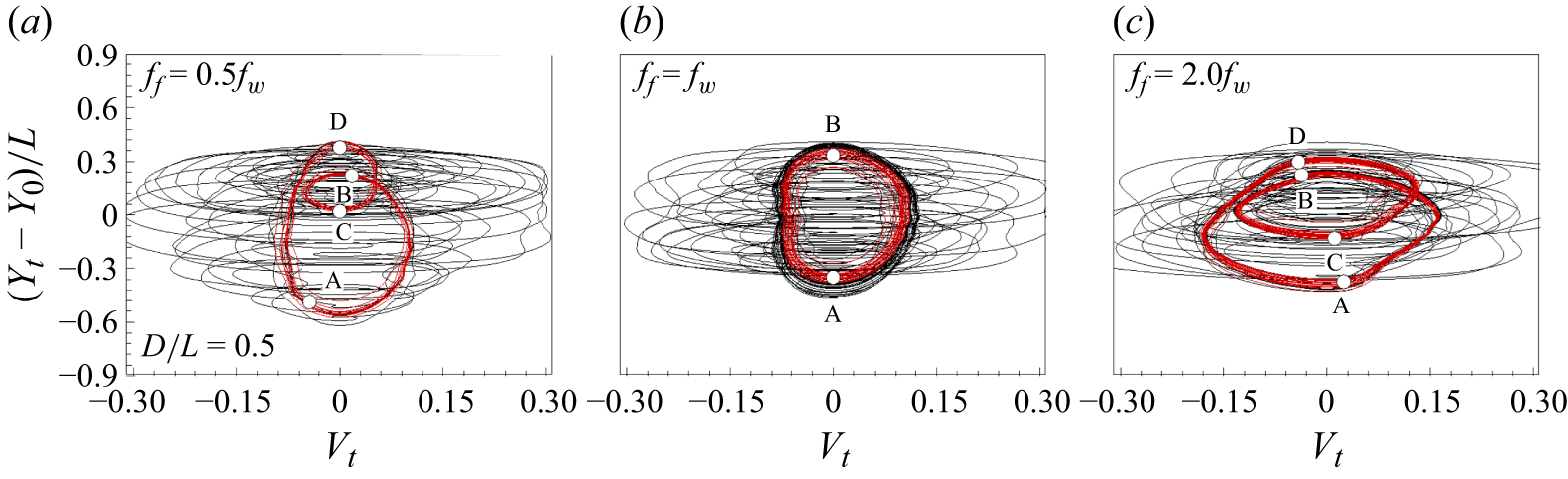
Phase diagram showing the relationship between the trailing-edge vertical displacement
 $Y_t$
and velocity
 $V_t$
for different heaving frequencies: (a)
 $f_{\!f} = 0.5f_w$
, (b)
 $f_{\!f} = f_w$
and (c)
 $f_{\!f} = 2.0f_w$
. The black lines denote the phase diagram for the initial transient periods, whereas the red lines represent the periodic converged state. The mean submergence depth is
 $D/L$
= 0.5, and the phase difference between the heaving motion and incident wave is
 $\mathit \varPhi$
= 0. The instants A–D correspond to the points in figure 2.

3.2. Effects of the ratio of heaving frequency to incident wave frequency and submergence depth
3.2.1. Foil kinematics and propulsive performance
The interaction dynamics between the flexible foil and incident wave is governed primarily by the ratio of the heaving frequency of the foil (
 $f_{\!f}$
) to the incident wave frequency (
 $f_w$
) and the submergence depth. At relatively low
 $f_{\!f}/f_w$
values, the foil’s kinematics and propulsive performance are largely influenced by wave-induced flow. In contrast, at high ratios, they become more sensitive to the actively imposed heaving motion rather than the wave-induced flow. In this section, we analyse how variations in the
 $f_{\!f}/f_w$
ratio affect foil kinematics and propulsive performance.
Figure 2 shows the histories of the leading-edge (blue solid line) and trailing-edge (red solid line)
 $y$
positions (figure 2
a–c) and vertical velocities (figure 2
d–f) for different heaving frequencies. The phase difference between the heaving motion and incident wave is
 $\mathit \varPhi$
= 0. The mean distance between the foil and the free surface is
 $D/L$
= 0.5. In figure 2(
 $b$
,
 $e$
), at
 $f_{\!f}$
=
 $f_w$
, a single mode is observed, whereas multiple modes are observed when
 $f_{\!f}$
= 0.5
 $f_w$
(in figure 2
 $a$
,
 $d$
) and 2.0
 $f_w$
(in figure 2
 $c$
,
 $f$
). As the heaving frequency increases, the vertical flapping velocities at the leading and trailing edges increase. Figure 3 displays the phase diagram between the trailing-edge vertical displacement
 $Y_t$
and velocity
 $V_t$
for various heaving frequencies. The black lines correspond to the initial transient periods, whereas the red lines represent the periodic converged state. In the presence of multiple modes in figure 3(a,c), the converged state leads to the formation of two loops. In figure 3(b), only a single closed loop is formed when
 $f_{\!f} = f_w$
. In figure 3(a), at
 $f_{\!f} = 0.5f_w$
, the loop shows an elongated shape in the
 $y$
axis, indicating a larger flapping amplitude of the trailing edge of the foil than in the cases of
 $f_{\!f} = f_w$
and
 $f_{\!f} = 2.0f_w$
. Figure 3(c) shows that increasing the heaving frequency to
 $2.0f_w$
raises the trailing-edge vertical velocity, elongating the phase diagram in the
 $x$
direction by approximately 71.57 % and 80.27 %, relative to the cases of
 $f_{\!f} = 0.5f_w$
and
 $f_{\!f} = f_w$
, respectively.
Same as for figure 2, but the mean submergence depth is
 $D/L$
= 2.0.


To illustrate the influence of the foil submergence depth and thus the wave effect, at another mean submergence depth of
 $D/L$
= 2.0, figures 4 and 5 show the histories of the leading- and trailing-edge
 $y$
positions (figure 4
a–c), vertical velocities (figure 4
d–f) and the corresponding phase diagram for different ratios of
 $f_{\!f} /f_w$
. According to wave theory for deep-water waves, the orbital velocity decreases exponentially as the depth increases. Interestingly, the multiple modes for
 $D/L$
= 0.5 and
 $f_{\!f} = 0.5f_w$
in figure 2(a,d) do not appear at
 $D/L$
= 2.0 in figure 4(a,d), and inflection points are observed instead of multiple modes, forming a single distorted loop, as visualised in figure 5(a). When the heaving frequency is smaller than that of the incident wave, the trailing-edge motion is significantly affected by the wave-induced flow. The trailing edge oscillates passively in response to the wave-induced flow, and the flapping amplitude and velocity decrease as
 $D/L$
increases, thereby reducing the size of the phase diagram in the
 $y$
direction. When
 $f_{\!f} = f_w$
, a single mode appears in figures 4(
 $b$
,
 $e$
) and 5(
 $b$
), similar to the case of
 $D/L$
= 0.5 in figures 2(
 $b$
,
 $e$
) and 3(
 $b$
). As
 $D/L$
increases from 0.5 to 2.0, a comparison of figures 2(
 $b$
,
 $e$
) and 4(
 $b$
,
 $e$
) reveals that the trailing edge’s amplitude and velocity increase because of the reduced wave effect. This result implies that the incident wave interferes with the flapping motion when
 $f_{\!f} = f_w$
and
 $\mathit \varPhi$
= 0. In figures 4(
 $c$
,
 $f$
) and 5(
 $c$
), at
 $f_{\!f}$
=
 $2f_w$
, multiple modes are observed, forming two loops. As
 $D/L$
increases at
 $f_{\!f}$
=
 $2f_w$
, the flapping amplitude and velocity slightly decrease, resulting in a reduced loop height in figure 5(
 $c$
) compared with that in figure 3(
 $c$
). In summary, as figures 2–
5 demonstrate, the interaction dynamics between the flexible foil and the incident wave is modulated by
 $f_{\!f}/f_w$
and
 $D/L$
, which play a significant role in determining the flapping kinematics and mode appearance.
Evolution of the flapping flexible foil in the wave field. The colour contours indicate the vertical component of the wave-induced velocity along the vertical line passing the foil’s leading edge as a function of time. The heaving frequency is (
 $a$
)
 $f_{\!f} = 0.5f_w$
, (
 $b$
)
 $f_{\!f} = f_w$
and (
 $c$
)
 $f_{\!f} = 2.0f_w$
. The thin black solid lines indicate the free surface, the thick black solid lines denote the foil’s configuration and the dashed lines represent the leading edge’s vertical trajectory as a function of time. The first, second and third rows of the dashed lines correspond to the cases of mean submergence depths of
 $D/L$
 $=$
0.5, 2.0 and 4.0, respectively. Note that because the wave propagates from left to right, the time evolution is from right to left, as indicated by the black arrow above each figure. The phase difference between the heaving motion and the incident wave is
 $\mathit \varPhi$
 $=$
0. The values under the foil represent the wave-induced vertical velocity at the leading edge.

We now proceed with the analysis of the wave-induced flow field surrounding the flexible foil to further examine the interaction dynamics in the parametric cases presented in figures 2–
5. Figure 6 shows the time evolution of the variation in the vertical velocity component of the flow along the vertical line passing the leading edge, highlighting how the flexible foil interacts with the wave-induced flow. The dashed line indicates the trajectory of the leading edge, and the three dashed lines correspond to the three mean depth cases of
 $D/L$
= 0.5, 2 and 4. The wave-induced velocity decreases exponentially as
 $D/L$
increases, as shown in figure 6. The values displayed under the foil indicate the wave-induced vertical velocity at the leading edge. In figure 6(
 $a$
), at
 $f_{\!f} = 0.5f_w$
, one cycle of the incident wave is completed during half of the full flapping cycle. The wave-induced flow assists the flapping motion of the flexible foil, increasing the trailing-edge amplitude near the wave surface. The instants in figure 6(
 $a$
) correspond to points A–D in figures 2(
 $a$
) and 3(
 $a$
), including
 $t$
= 7.27 (A), 7.43 (B), 7.5 (C) and 7.61 (D). During the upstroke period of the leading edge (A–B;
 $t$
= 7.27–7.43), its velocity is comparable to the wave-induced flow velocity in the vertical direction as shown in figures 2(
 $d$
) and 6(
 $a$
). The foil is largely influenced by wave-induced upward flow, causing notable upward motion of the trailing edge. In the subsequent phase (B–C;
 $t$
= 7.43–7.50), the leading-edge vertical velocity decreases and the foil encounters the wave-induced downward flow (in figures 2
 $d$
and 6
 $a$
), which causes a decrease in the
 $y$
position of the trailing edge, resulting in a small loop in the phase diagram shown in figure 3(
 $a$
). As the leading edge undergoes its downstroke during the C–D (
 $t$
= 7.50–7.61) period, its vertical velocity increases and becomes comparable to the wave-induced vertical velocity (in figures 2
 $d$
and 6
 $a$
). The foil encounters an upward flow, causing the
 $y$
position of the trailing edge to rise and reach its highest point on the phase diagram (figure 3
 $a$
). The trailing edge subsequently undergoes significant descending movement due to the combined effect of the downward motion of the leading edge and the downward flow induced by the incident wave, resulting in a vertically elongated shape in the phase diagram (figure 3
 $a$
). As the submergence depth
 $D/L$
increases, the reduced influence of the wave effect (figure 6
 $a$
) alters the phase diagram, causing the double-loop shape observed near the surface to disappear (figures 3
 $a$
and 5
 $a$
).
Next, figure 6(
 $b$
) depicts the case of
 $f_{\!f}$
 $=$
 $f_w$
. The phase difference
 $\mathit \varPhi$
between the heaving motion and the vertically wave-induced flow is set to zero, which leads to the same phase between the slope of the dashed line and the
 $v$
-velocity contours in figure 6(
 $b$
). During the upstroke (instant A in figure 6
 $b$
) and downstroke (instant B in figure 6
 $b$
) of the leading edge, its vertical velocity is similar to the wave-induced vertical velocity, as shown in figures 2(
 $e$
) and 6(
 $b$
). The fluctuation initiated by the sinusoidal boundary condition at the leading edge propagates along the flexible foil, resulting in a phase difference between the motions of the leading and trailing edges, as shown in figure 4(
 $b$
). Owing to this phase difference, the posterior parts of the foil oscillate with a delayed motion with respect to the wave-induced vertical flow, decreasing the flapping amplitude as the foil approaches the wave surface.
When the heaving frequency increases to
 $f_{\!f} = 2.0f_w$
, as shown in figure 6(
 $c$
), the foil has two flapping cycles in a wave period. At this higher frequency, the motion of the trailing edge is influenced primarily by the sinusoidal boundary condition imposed on the leading edge rather than by wave-induced flow. Consequently, the flapping kinematics are not significantly affected by the submergence depth
 $D/L$
, as illustrated in figure 6(
 $c$
). The phase diagram in the converged state, shown in figure 3(
 $c$
), consists of two modes. The first mode, A–B–C, corresponds to a larger oscillation, and the second mode, C–D–A, represents a smaller oscillation. In the first mode, the foil encounters a negative wave-induced velocity while flapping. In figure 6(
 $c$
), at the early stage of the downstroke (
 $t$
= 7.31) in the first mode, the leading-edge vertical velocity decreases as the wave-induced negative velocity reaches its maximum. The wave-induced negative vertical flow assists the downward motion of the trailing edge. As a result, in figure 3(c), the phase diagram for the first mode is biased downward. During the downstroke of the first mode (
 $t$
= 7.34–7.38), the heaving velocity of the leading edge is larger than the wave-induced flow velocity in the vertical direction (figures 2
 $f$
and 6
 $c$
). The wave-induced negative velocity hinders the upward motion of the trailing edge. During the upstroke of the first mode (
 $t$
= 7.38–7.43), the leading-edge vertical velocity decreases and the foil encounters the maximum positive wave-induced velocity at instant C (figures 2
 $f$
and 6
 $c$
). The wave-induced positive velocity retards the downward bending of the trailing edge. During the second mode’s downstroke (
 $t$
= 7.43–7.49), the leading-edge velocity reaches its maximum and is greater than the wave-induced velocity at
 $t$
= 7.47 (figures 2
 $f$
and 6
 $c$
). The wave-induced positive velocity helps bend the trailing edge upward. As a result, the phase diagram for the second mode is biased upward compared with that for the first mode. As
 $D/L$
increases, the wave effect that creates the additional deformation decreases, by which the two loops become more similar in figure 5(
 $c$
) than in figure 3(
 $c$
).
Variations in (
 $a$
) the trailing edge’s
 $y$
amplitude, (
 $b$
) the time-averaged thrust coefficient, (
 $c$
) the time-averaged power coefficient and (
 $d$
) the propulsive efficiency with the mean submergence depth
 $D/L$
. The red, green and blue lines denote the cases of
 $f_{\!f} = 0.5f_w$
,
 $f_w$
and
 $2.0f_w$
, respectively. The dashed lines represent the case
 $D/L = \infty$
, where the results are independent of the incident wave or free-surface parameters. The phase difference between the heaving motion and the incident wave is
 $\mathit \varPhi$
 $=$
0.

According to wave theory (Airy Reference Airy1845), the magnitude of wave-induced flow decreases as
 $D/L$
increases (figure 6), resulting in the flexible foil being less affected by the incident wave. When
 $\mathit \varPhi$
= 0, the flapping motion increases and decreases near the wave surface at
 $f_{\!f}/f_w$
values of 0.5 and 1.0, respectively. As the
 $f_{\!f}/f_w$
ratio reaches 2.0, the flapping motion becomes less affected by the incident wave than are the other two ratio cases. The hydrodynamic benefits or hindrances associated with being near the wave surface, in terms of propulsive performance, are closely related to the interaction dynamics between the flexible foil and the wave-induced flow. To qualitatively understand how the interaction dynamics affects propulsive performance, we adopt the thrust coefficient
 $C_T$
and lift coefficient
 $C_L$
, defined as
 \begin{equation} C_T = \frac {\int _0^1 F_x(s,t) \text{d}s}{\dfrac {1}{2} \rho u_\infty ^2 dL}, \quad C_L = \dfrac {\int _0^1 F_y(s,t) \text{d}s}{\dfrac {1}{2} \rho u_\infty ^2 dL}. \end{equation}
The time-averaged thrust coefficient and power coefficient are calculated by
 \begin{equation} \overline {C_T} = \frac {\dfrac {1}{T} \int _t^{t+T} \int _0^1 F_x(s,t) \text{d}s \text{d}t}{\dfrac {1}{2} \rho u_\infty ^2 dL}, \quad \overline {C_P} = \dfrac {\dfrac {1}{T} \int _t^{t+T} \int _0^1 F_y(s,t) \dfrac {\partial Y(s,t)}{\partial t} \text{d}s \text{d}t}{\dfrac {1}{2} \rho u_\infty ^3 dL}. \end{equation}
The leading-edge motion is prescribed as a sinusoidal heaving motion, while the posterior parts of the foil respond dynamically through their interaction with the wave-induced flow. Thus, the power coefficient in (3.2) is calculated based on the input power required by the flapping motion of the entire flexible body against the surrounding fluid. Figure 7 shows the normalised trailing-edge amplitude
 $A_t/L$
, time-averaged thrust coefficient
 $\overline {C_T}$
, power coefficient
 $\overline {C_P}$
and propulsive efficiency
 $\eta = {\overline {C_T}}/{\overline {C_P}}$
(Anderson et al. Reference Anderson, Streitlien, Barrett and Triantafyllou1998). The dashed lines indicate the values obtained from the simulation without the surface wave. At
 $D/L$
= 6.0, the wave-induced velocity is insignificant. As a result, the thrust coefficient, power coefficient and propulsive efficiency at
 $D/L$
= 6.0 are similar to those of the case without the surface wave. In figure 7(
 $a$
), as
 $D/L$
decreases, the flapping amplitude decreases at
 $f_{\!f} = f_w$
, whereas it increases at
 $f_{\!f} = 0.5f_w$
. The flapping amplitude increases with decreasing submergence depth at
 $f_{\!f} = 2.0f_w$
, but the amplitude variation with depth is less sensitive than that in other frequency cases, as discussed earlier. Figure 7(
 $b$
) displays the time-averaged thrust coefficient. Notably, the influence of the incident wave on thrust generation depends on the ratio
 $f_{\!f}/f_w$
. As
 $D/L$
decreases, the thrust coefficient increases at
 $f_{\!f} = 0.5f_w$
, whereas it diminishes at
 $f_{\!f} = f_w$
and
 $f_{\!f} = 2.0f_w$
. The input power required for the flapping motion is obtained by integrating the product of the hydrodynamic force in the
 $y$
direction and the trailing-edge vertical velocity, as defined in (3.2). Thus, a greater elongation in the phase diagram in the
 $x$
direction as discussed in figures 3 and 5 correlates with higher input power. However, because the hydrodynamic force also varies with the ratio
 $f_{\!f}$
/
 $f_w$
, the elongation does not translate directly into the relative increase in the power coefficient presented in figure 7. On the basis of both the thrust and the input power, the optimal submergence depth for propulsive efficiency is approximately
 $D/L$
= 1.0 when
 $f_{\!f} = 0.5f_w$
, as shown in figure 7(
 $d$
). As the submergence depth further increases, the efficiency decreases. In contrast, the foil flapping with
 $f_{\!f} = f_w$
is hindered near the wave surface from the viewpoint of the propulsive efficiency (figure 7
 $d$
). At the frequency
 $f_{\!f} = 2.0f_w$
, the thrust, the power input and the resulting propulsive efficiency show only slight variations with changes in
 $D/L$
. The trends of the kinematics and propulsive performance, which varies with
 $D/L$
for different
 $f_{\!f} /f_w$
, at the higher Reynolds numbers of 200 and 400 resemble those observed at
 $Re$
= 100 plotted in figure 7 (see supplementary materials available at https://doi.org/10.1017/jfm.2025.10705).
The decreasing trends of the thrust coefficient and propulsive efficiency as the foil approaches the wave surface at
 $f_{\!f} = f_w$
are inconsistent with what was reported by Liu et al. (Reference Liu, Liu, Huang, Zhao and Su2018), where the effect of an incident wave on propulsive performance was numerically investigated for a rigid foil and a foil with a prescribed deformation. In their study, the thrust coefficient increased near the wave surface at
 $f_{\!f} = f_w$
for both the rigid foil and the prescribed deformation cases. This discrepancy is likely attributed to the dynamic deformation of the flexible foil. In the present study, when
 $f_{\!f} = f_w$
and
 $\mathit \varPhi$
= 0, the interaction between the foil and the wave-induced flow results in a notable reduction in the trailing-edge amplitude (
 $A_t$
) and thrust coefficient (
 $C_T$
) near the wave surface. This reduction suggests that the foil’s dynamic response to the incident wave is crucial in determining the propulsive performance. Specifically, the dynamic deformation may cause local modifications in the flow field around the foil, altering the unsteady forces that impact thrust generation and propulsive efficiency. These effects are examined in detail in the subsequent discussion on vortex dynamics.
Variations in (
 $a$
)
 $C_T$
and (
 $b$
)
 $C_L$
with time. The dashed lines indicate the mean values. The instants A–D in (
 $a$
,
 $b$
) correspond to those in figure 3(
 $a$
). (A–D) Instantaneous vorticity field at instants A–D with a subset of the magnified view near the foil. Vortices 1
 $-$
4 are discussed in the text. The heaving frequency is
 $f_{\!f} = 0.5f_w$
, the mean submergence depth is
 $D/L$
= 0.5 and the phase difference between the heaving motion and incident wave is
 $\mathit \varPhi$
= 0.

3.2.2. Vortex dynamics and propulsion
To better understand the underlying mechanisms of the hydrodynamic benefits or hindrances experienced by the flexible foil near the wave surface, we now investigate the time variation in the hydrodynamic force coefficient in the context of the vortex structures. The vortices are generated by the combined effect of the foil’s flapping motion and the wave-induced flow. Figure 8(a,b) shows the
 $x$
and
 $y$
components of the hydrodynamic force coefficients acting on the flexible foil flapping with
 $f_{\!f} = 0.5f_w$
at
 $D/L$
= 0.5. The instants A–D correspond to those in figures 2(
 $a$
) and 3(
 $a$
), during which the vorticity fields are visualised in figure 8(A–D). During the upstroke, the first and second modes of foil deformation are induced by the wave-induced velocity, as depicted in figure 3(
 $a$
), which correspond to the D–A–B and B–C–D periods, respectively. At instant A, the trailing edge reaches the lowest
 $y$
position, and a negative shear layer develops on the upper surface of the foil, as shown in figure 8(A). A vortex structure with positive
 $\omega _z$
(hereafter called a positive vortex), labelled 1 in figure 8, sheds during the previous downstroke. In the following upstroke from A to B, the negative shear layer (i.e. with negative
 $\omega _z$
) is detached from the trailing edge, forming a coherent negative vortex labelled 2. This upstroke is driven mainly by the sinusoidal heaving motion imposed at the leading edge. Then, the trailing edge undergoes a minor downstroke from B to C, driven by the incident wave. A weak positive vortex (labelled 3) is generated and merges with vortex 1. The size of the merged positive vortex structure (labelled 1 + 3 in D) is increased, potentially enhancing the thrust on the foil. The remaining upstroke occurs in the C to D period, shedding negative vortex 4 with a V shape. Figure 8(
 $b$
) shows the history of the lift force coefficient on the foil, which is closely related to the motion of the foil; it locally decreases and increases during the upstroke and downstroke of the foil, respectively.


To examine the submergence depth effect, the results for the same
 $f_{\!f} = 0.5f_w$
but at a different
 $D/L$
= 2.0 are plotted in figure 9 for comparison with figure 8. The wave-induced velocity decreases exponentially as the depth increases, which explains why the first and second modes shown in figure 8 disappear in figure 9 far from the wave surface (see also figures 2–5). Instead, as shown in figure 9(
 $a$
), the thrust generation is almost zero when inflection point B in figure 4(
 $a$
) occurs. Figure 9(A,C) shows how the upstroke and downstroke create positive and negative vortices, respectively. Owing to the smaller flapping amplitude at
 $D/L$
= 2.0 than at
 $D/L$
= 0.5, the strength and size of the alternating vortex structures consisting of a reverse Kármán vortex street decrease, resulting in less thrust generation. The velocity induced by the vortex–vortex interaction is directed in the positive
 $x$
direction, forming a horizontal jet in the wake of the foil, as visualised in the phase-averaged
 $u$
field in figure 9(A
 $'$
,C
 $'$
). Figure 9(
 $b$
) displays the history of
 $C_L$
, which decreases from A to D during the upstroke with a local increment near the inflection point B. Because the foil is away from the wave surface, the average force coefficient in the
 $y$
direction is close to zero (approximately
 $-$
0.076).
Same as figure 8, but at a frequency ratio of
 $f_{\!f} = f_w$
. (A,B) Instantaneous vorticity fields and (A
 $'$
,B
 $'$
) phase-averaged
 $u$
fields at instants A and B. Instants A and B correspond to those in figures 2(
 $b$
) and 3(
 $b$
). The black arrow indicates the direction of the flow induced by the vortex structure.

Next, we examine the effect of the frequency ratio
 $f_{\!f}/f_w$
. To compare with the
 $f_{\!f} = 0.5f_w$
case shown in figure 8, figure 10 presents the results at
 $f_{\!f} = f_w$
and
 $D/L$
= 0.5, in which case the average thrust coefficient over the flapping cycle is negative (figure 10
 $a$
). In figure 10(
 $b$
), the lift coefficient increases and decreases during the upstroke (instant A) and downstroke (instant B), respectively. The instants A and B correspond to those in figures 2(
 $b$
) and 3(
 $b$
), where a single flapping mode is observed. At instant A, the horizontal and vertical components of the wave-induced velocity near the trailing edge are negative and positive, respectively. In figure 10(A), the positive vortex structure generated during the downstroke is divided into two parts due to the interaction between the wave-induced flow and the foil’s flapping motion. One part, labelled 1, rolls between the wave surface and the upper part of the foil, whereas the other part, labelled 2, remains below the foil. During the upstroke A–B, as plotted in figure 10(b), the negative vortex splits into vortices 3 and 4, whereas the thrust coefficient reaches a minimal negative value (figure 10
 $a$
).
The interaction between vortices 1 and 3 induces an upstream flow, forming a drag wake. This phenomenon is visualised in the phase-averaged streamwise velocity field in figure 10(A
 $'$
), where an upstream flow with negative
 $u$
is induced near the wave surface. Similarly, a drag wake (denoted by the black arrow) is induced by vortices 2 and 3 in figure 10(A) and vortices 2 and 4 in figure 10(B). This result explains why a flexible foil, flapping with
 $f_{\!f} = f_w$
near wave surface, has a lower propulsive efficiency than one far from the surface. In summary, the vortex structures formed near the foil due to the combined effect of wave-induced flow and heaving motion interact with each other to induce an upstream flow, resembling a drag wake.


We now proceed to analyse at
 $f_{\!f}=f_w$
how the characteristics of the vortex structures vary with increasing
 $D/L$
, as shown in figure 11. As
 $D/L$
increases from 0.5 to 2.0, the thrust becomes positive, as shown in figures 10(
 $a$
) and 11(
 $a$
), and the lift coefficient increases, as illustrated in figures 10(
 $b$
) and 11(
 $b$
). Although the vortex roll-up phenomenon is mitigated with increasing
 $D/L$
and decreasing wave-induced velocity, the positive and negative vortices generated during the downstroke and upstroke are split into two parts. The positive vortex is divided into vortices 1 and 2 in figure 11(A), whereas the negative vortex is divided into vortices 3 and 4 in figure 11(B). The main vortex structures 1 and 4 drift downstream and contribute to thrust generation by forming a reverse Kármán vortex street. On the other hand, vortices 2 and 3 remain below and above the foil, respectively. During the downstroke, negative vortex 3 interacts with positive vortex 1 before shedding downstream, producing a drag wake above the foil. The vortex–vortex interaction between vortices 2 and 4 also induces an upstream jet near the lower part of the foil during the upstroke, also producing a drag wake.
The above-mentioned drag wakes occurring during the upstroke and downstroke are visualised in the phase-averaged streamwise velocity fields in figures 11(A
 $'$
) and 11(B
 $'$
). In the central region, a strong jet wake (with positive
 $u$
) is produced by the reverse Kármán vortex street consisting of the series of main vortex structures 1 and 4, whereas a drag wake (with negative
 $u$
) appears above and below the foil. This result indicates that the wave-induced velocity affects vortex dynamics even at
 $D/L$
= 2.0 and interferes with thrust generation by splitting the vortex structures. The thrust coefficient increases as
 $D/L$
increases and saturates at approximately
 $D/L$
= 5.0, as shown in figure 7(
 $b$
). Beyond this point, the vortex-splitting phenomenon disappears, and the foil generates a thrust wake without a nearby drag wake. The same vortex dynamics and the mechanisms of the thrust enhancement and reduction described above persist at the higher Reynolds numbers of 200 and 400, as shown in the supplementary material.
The wave-induced flow patterns in the vertical direction are similar to those observed in a reverse Kármán vortex street. Park & Sung (Reference Park and Sung2018) conducted simulations of two tandem self-propelled flexible foils to investigate the flow-mediated interactions between them. They reported that the two flexible foils dynamically form a stable tandem configuration, where the motion of the downstream foil’s leading edge is in phase with the vertical flow induced by the oncoming vortices shed from the upstream foil. In the vertical direction, positive and negative velocities are alternately induced by the vortices, resembling the flow patterns generated by incident waves studied here. However, in the horizontal direction, the upstream foil generates a thrust wake, whereas the incident wave induces alternating positive and negative horizontal velocities, which affect the propulsive performance of the flexible foil flapping near the wave surface as shown in figures 8 and 10.
Same as figure 6, but for the phase differences between the heaving motion and incident wave of (
 $a$
)
 $\mathit \varPhi$
 $=$
 $\pi$
/4 and (
 $b$
)
 $\mathit \varPhi$
 $=$
 $\pi$
.

We now summarise
 $\S$
3.2. In this section, we focus primarily on the effects of
 $f_{\!f}/f_w$
and
 $D/L$
on the propulsive performance of the flexible foil beneath the wave surface. Previous studies by Wu (Reference Wu1972) and Liu et al. (Reference Liu, Liu, Huang, Zhao and Su2018) reported that the thrust and propulsive efficiency of rigid foils and foils with prescribed deformation were optimised at
 $f_{\!f}/f_w$
= 1.0. In contrast, our study, which considers the dynamic deformation of a flexible foil interacting with wave-induced flow, shows that the propulsive performance decreases near the wave surface due to the presence of a drag wake. This drag wake is generated by the combined effect of the foil’s flapping motion and the wave-induced flow. In other words, wave-induced flow affects the vortex dynamics near the flexible foil, thereby affecting the propulsive performance. This result suggests that the drag wake can be modulated by adjusting the phase difference between the heaving motion and the wave-induced flow to improve the propulsive performance, which is discussed in
 $\S$
3.3.
3.3. Effects of the phase difference between the heaving motion and incident wave on the propulsive performance of foil
In this section, we focus on the effect of the phase difference between the foil heaving motion and the incident wave (
 $\mathit \varPhi$
) on the kinematics, vortex dynamics and propulsive performance of the flexible foil. Figures 12(
 $a$
) and 12(
 $b$
) present the time evolution of the variation in the vertical flow velocity along the vertical line passing the leading edge at
 $\mathit \varPhi$
=
 $\pi /4$
and
 $\pi$
, respectively. At
 $\mathit \varPhi$
= 0, the wave-induced flow hinders the trailing-edge motion during most of the upstroke and downstroke periods (figure 6
 $b$
). When
 $\mathit \varPhi$
increases from 0 to
 $\pi$
/4 in figure 12(
 $a$
), at the early stage of the downstroke (
 $t$
= 7.25) and the upstroke (
 $t$
= 7.37) of the leading edge, the wave-induced velocity helps bend the trailing edge upward and downward, respectively. Apart from the early stage of each downstroke and upstroke, the wave-induced flow hinders the trailing-edge motion, similar to the case at
 $\mathit \varPhi$
= 0. When
 $\mathit \varPhi$
increases to
 $\pi$
(figure 12
 $b$
), the wave-induced vertical flow generally assists the trailing-edge motion during the flapping period, thereby increasing the trailing-edge amplitude as the foil approaches the wave surface.
Variations in (
 $a$
) the trailing-edge amplitude, (
 $b$
) the time-averaged thrust coefficient, (
 $c$
) the time-averaged power coefficient and (
 $d$
) the propulsive efficiency for different phase differences between the heaving motion and the incident wave,
 $\mathit \varPhi$
. The red, blue, black and green lines denote
 $D/L$
values of 0.5, 1.0, 2.0 and 4.0, respectively. The heaving frequency (
 $f_{\!f}$
) matches that of the incident wave (
 $f_w$
) in each case.

Figure 13 shows the trends of the trailing-edge amplitude, thrust coefficient, power coefficient and propulsive efficiency with various
 $\mathit \varPhi$
and
 $D/L$
values at
 $f_{\!f} = f_w$
. When
 $\mathit \varPhi$
changes from 0 to
 $\pi$
/4, the flapping amplitude of the trailing edge increases by 35.19 % and 22.69 % at
 $D/L$
= 0.5 and 1.0, respectively. The amplitude continues to increase gradually until
 $\mathit \varPhi$
=
 $\pi$
and then decreases as the phase difference further increases. At
 $D/L$
= 4.0, the flapping amplitude remains relatively constant with variations in the phase difference, indicating a decrease in the wave effect in deep water. The thrust coefficient and power coefficient in figure 13(
 $b, c$
) exhibit a trend similar to that of the flapping amplitude with respect to the phase difference dependence. They increase first and then decrease as
 $\mathit \varPhi$
increases, with a local peak appearing at approximately
 $\mathit \varPhi$
=
 $\pi$
for each submergence depth. Figure 13(
 $d$
) shows the propulsive efficiency, considering both the thrust and the input power. At
 $D/L$
= 0.5, the maximum propulsive efficiency occurs at
 $\mathit \varPhi$
=
 $\pi$
, whereas it occurs at
 $\mathit \varPhi$
= 5
 $\pi$
/4 for
 $D/L$
= 1.0. In most phase difference cases, the propulsive efficiency decreases as the foil approaches the wave surface. When the foil is submerged deeply at
 $D/L$
= 4.0, wave-induced flow with different phase differences only slightly affects the efficiency.
Filippas & Belibassakis (Reference Filippas and Belibassakis2014) used a boundary-element method to investigate the hydrodynamic effect of surface waves on a rigid foil. Their results indicated the importance of adjusting the phase difference
 $\mathit \varPhi$
to achieve high performance. For the foil flapping near the wave surface, at the frequency of
 $f_{\!f} = f_w$
, thrust is maximised and minimised when the leading edge’s heaving motion is out of phase and in phase with the wave-induced vertical flow, respectively. Consistently, in the present study at
 $D/L$
= 0.5, the maximum and minimum thrust are observed when the heaving motion is out of phase (
 $\mathit \varPhi = \pi$
, figure 12
 $b$
) and in phase (
 $\mathit \varPhi$
= 0, figure 6
 $b$
) with the wave-induced vertical flow, respectively. However, regarding the influence of submergence depth on thrust, the trends identified in figure 13(
 $b$
) differ from those reported by Filippas & Belibassakis (Reference Filippas and Belibassakis2014), where the rigid foil flapping with an optimal phase difference produces greater thrust near the wave surface than farther from it. This trend is not observed in our simulation because of the vortex-splitting mechanisms, which are further discussed below.
Variation in (
 $a$
)
 $C_T$
and (
 $b$
)
 $C_L$
with time. The dashed line shows
 $\overline {C}_T$
in (a) and
 $\overline {C}_L$
in (b). The subset shows the history of the trailing edge’s
 $y$
position. Instants A and B indicate the phase where the trailing edge’s amplitude reaches the minimum and maximum values, respectively. (A,B) Instantaneous vorticity field at instants A and B and (A
 $'$
,B
 $'$
) phase-averaged
 $u$
fields at instants A and B. The heaving frequency (
 $f_{\!f}$
) matches the incident wave frequency (
 $f_w$
), the mean submergence depth is
 $D/L$
= 0.5 and the phase difference between the heaving motion and the incident wave is
 $\mathit \varPhi$
=
 $\pi$
/4.

Same as figure 14, but at
 $\mathit \varPhi$
=
 $\pi$
.

Next, we investigate the vortex dynamics surrounding the flexible foil. To reveal how the vortex–foil interaction and the resulting propulsive performance vary with
 $\mathit \varPhi$
when the foil is near the wave surface (
 $D/L$
= 0.5), we compare
 $C_T$
,
 $C_L$
and the vorticity field at
 $\mathit \varPhi$
=
 $\pi$
/4 and
 $\pi$
, as shown in figures 14 and 15, respectively. Figures 14(a) and 14(b) display the time evolution of
 $C_T$
and
 $C_L$
, respectively, with a subset indicating the history of the
 $y$
position of the trailing edge of the foil. The mean values of the thrust and lift coefficients over the flapping cycle are negative. Figures 14(A) and 14(B) present the vorticity field at instants A and B in figure 14(
 $a$
), respectively, where the vortex roll-up and splitting phenomena occur similarly to the case of
 $\mathit \varPhi$
= 0 in figure 10. Compared with the
 $\mathit \varPhi$
= 0 case, positive vortex 1 is induced further upstream and trapped between the wave surface and foil. Figure 13(a,b) shows that at
 $D/L$
= 0.5, despite a significant increase in the flapping amplitude from
 $\mathit \varPhi$
= 0 to
 $\pi$
/4, the thrust decreases slightly; at
 $D/L$
= 1.0, there is a significant reduction in the thrust despite a 22.69 % increase in the flapping amplitude. This result implies that the vortex–vortex and vortex–foil interactions occurring at
 $f_{\!f} = f_w$
and
 $\mathit \varPhi$
=
 $\pi$
/4 have a detrimental effect on thrust generation and do not contribute to improving propulsive efficiency. However, the vortex roll-up phenomenon observed at
 $\mathit \varPhi$
= 0 (in figure 10) and
 $\pi$
/4 (in figure 14) is mitigated as
 $\mathit \varPhi$
increases to
 $\pi$
in figure 15.
Figure 15 shows the vorticity field and the phase-averaged
 $u$
field at
 $D/L$
= 0.5 and
 $\mathit \varPhi$
=
 $\pi$
at instants A and B in figure 15(a,b). The aforementioned vortex-splitting phenomenon is also observed in this parametric set-up. The positive vortex structure generated during the downstroke is divided into vortices 1 and 2 in figure 15(A), and the negative vortex structure is split into vortices 2 and 4 in figure 15(B). Immediately behind the foil, the vortex–vortex interactions between vortices 2 and 4 and between vortices 1 and 3 generate a drag wake, as shown in the time-averaged velocity field in figure 15 (A
 $'$
,B
 $'$
). The induced negative velocity is observed near the wave surface and below the foil in figure 15(A
 $'$
), as denoted by the dashed contour line corresponding to
 $u$
= 0. The strength of the drag wake decreases as
 $D/L$
increases, mitigating vortex splitting and increasing the thrust, as shown in figure 13(
 $b$
). When the phase difference increases from
 $\mathit \varPhi$
=
 $\pi$
/4 to
 $\pi$
, the main difference is that the vortex roll-up phenomenon caused by the wave-induced velocity in figure 14 disappears in figure 15. Instead, vortices 1 and 4 drift downstream, forming a reverse Kármán street (figure 15). As a result, a strong jet is produced in the wake of the foil (figure 15), allowing the foil to generate a positive thrust with an improvement in the propulsive efficiency, as shown in figure 13. When the phase difference further increases from
 $\pi$
to 7
 $\pi$
/4, the flapping amplitude decreases, as indicated in figure 13(
 $a$
), and the vorticity strength decreases (not plotted here), leading to a decrease in thrust generation, as shown in figure 13(
 $b$
).
Next, we examine the effect of the heaving–wave phase difference
 $\mathit \varPhi$
on the propulsive performance at
 $f_{\!f}/f_w$
= 0.5. In figure 7(
 $d$
), at
 $\mathit{\varPhi }=0$
, the optimal submergence depth for maximising the propulsive efficiency is
 $D/L$
= 1 when the foil flaps with
 $f_{\!f} = 0.5f_w$
. The effects of the phase difference on the foil’s kinematics and propulsive efficiency are analysed in figures 16–18 for
 $D/L$
= 1 and
 $f_{\!f} = 0.5f_w$
. Figure 16 displays the histories of the leading- and trailing-edge
 $y$
positions at various phase differences, for which the corresponding phase diagrams are visualised in figure 17. In figure 17(
 $a$
), compared with figure 3(
 $a$
) at
 $D/L$
= 0.5, the multiple modes do not entirely disappear, but the size of the additional mode corresponding to the B–C–D period diminishes as
 $D/L$
increases from 0.5 to 1.0. Point D indicates the local maximum of the trailing-edge
 $y$
position caused by wave-induced flow. As depicted in figures 16 and 17, the
 $y$
-position value of point D decreases as the phase difference increases from 0 to
 $\pi$
/2 and then increases as the phase difference further increases to 5
 $\pi$
/8 and 3
 $\pi$
/4. Specifically, at
 $\mathit \varPhi$
=
 $\pi$
/2, point D becomes an inflection point rather than a local maximum (figure 16
 $d$
), and the flapping mode approaches a single loop (figure 17
 $d$
), resulting in a larger flapping amplitude than in other cases.
Histories of the leading-edge (blue solid line) and trailing-edge (red solid line)
 $y$
positions for various phase differences: (
 $a$
)
 $\mathit \varPhi$
= 0, (
 $b$
)
 $\mathit \varPhi$
=
 $\pi$
/8, (
 $c$
)
 $\mathit \varPhi$
=
 $\pi$
/4, (
 $d$
)
 $\mathit \varPhi$
=
 $\pi$
/2, (
 $e$
)
 $\mathit \varPhi$
= 5
 $\pi$
/8 and (
 $f$
)
 $\mathit \varPhi$
= 3
 $\pi$
/4. The black dashed line presents the times corresponding to instants A–D. The instants A–D indicate the local minimum or maximum of the trailing edge’s
 $y$
position. The mean submergence depth is
 $D/L$
= 1.0, and the heaving frequency is half the incident wave frequency, i.e.
 $f_{\!f} /f_w$
= 0.5.

Phase diagram showing the relationship between the trailing-edge displacement
 $Y_t$
and velocity
 $V_t$
for various phase differences: (
 $a$
)
 $\mathit \varPhi$
= 0, (
 $b$
)
 $\mathit \varPhi$
=
 $\pi$
/8, (
 $c$
)
 $\mathit \varPhi$
=
 $\pi$
/4, (
 $d$
)
 $\mathit \varPhi$
=
 $\pi$
/2, (
 $e$
)
 $\mathit \varPhi$
= 5
 $\pi$
/8 and (
 $f$
)
 $\mathit \varPhi$
= 3
 $\pi$
/4. The instants A–D correspond to those in figure 16. The mean submergence depth is
 $D/L$
= 1.0, and the heaving frequency is half the incident wave frequency, i.e.
 $ f_{\!f} /f_w = 0.5$
.

Variations in (
 $a$
) the trailing-edge amplitude, (
 $b$
) the time-averaged thrust coefficient, (
 $c$
) the time-averaged input power coefficient and (
 $d$
) the propulsive efficiency with the phase difference between the heaving motion and incident wave. The red, blue, black and green lines denote the cases where
 $D/L$
= 0.5, 1.0, 2.0 and 4.0, respectively. The heaving frequency is half the incident wave frequency, i.e.
 $f_{\!f} /f_w = 0.5$
.

In the phase diagram shown in figure 17, the converged state is denoted by red lines. Secondary small loops (e.g. B–C in figure 17
 $a$
) are generated because of the presence of multiple flapping modes. At
 $\mathit \varPhi$
=
 $\pi$
/2, the secondary loop disappears, and the size of the main loop is larger than that in other cases. Similar to the cases at
 $f_{\!f} /f_w = 1$
in figures 13–15, figures 16 and 17 demonstrate that both the flapping kinematics and the phase diagram at
 $f_{\!f} /f_w = 0.5$
are largely influenced by
 $\mathit \varPhi$
. To examine how the modulated flapping kinematics, adjusted by varying
 $\mathit \varPhi$
, affect the hydrodynamic benefits or hindrances for being near the surface, next, we discuss the dependence of the propulsive performance on
 $\mathit \varPhi$
and
 $D/L$
, as plotted in figure 18.
In figure 18(
 $a$
), the flapping amplitude exhibits a cyclic trend with the phase difference, featuring a local peak at approximately
 $\mathit \varPhi$
= 3
 $\pi$
/8 and
 $\pi$
/2. In figure 18(b,c), the thrust coefficient and power coefficient display a trend similar to that of the flapping amplitude. Figure 18(
 $d$
) presents the propulsive efficiency based on the input power and thrust, highlighting the optimal submergence depth at
 $D/L$
= 1.0. Additionally, a favourable phase difference for achieving high efficiency is observed at
 $\mathit \varPhi$
= 0 and
 $\pi$
/2 for
 $f_{\!f} = 0.5f_w$
.
We now summarise
 $\S$
3.3. In this section, we demonstrate how the phase difference
 $\mathit \varPhi$
affects the foil’s kinematics, vortex dynamics and propulsive performance. The results indicate that
 $\mathit \varPhi$
plays a crucial role in affecting the hydrodynamic interaction between the wave and flexible foil through the surrounding vortex dynamics. Therefore,
 $\mathit \varPhi$
should be properly adjusted considering
 $f_{\!f} / f_w$
and
 $D/L$
to optimise the thrust and efficiency.
(
 $a$
) Schematic diagram of the flexible foil near the wave surface. The solid line denotes a foil’s configuration from which the angle of attack
 $\alpha$
is measured. The free-stream velocity is denoted by
 $u_\infty$
. The velocity of the leading edge in the
 $y$
direction is denoted by
 $\dot Y_l$
. The free-stream velocity combined with the wave-induced velocity relative to the heaving motion of the foil is represented by an effective velocity
 $u_{\textit {eff}}$
. (
 $b$
) Superimposed configurations of the flexible foil with separated heaving and pitching motions. The
 $y$
amplitude of the sinusoidal heaving motion at the leading edge is denoted by
 $A_{\!f}$
and the trailing-edge amplitude is denoted by
 $A_t$
. Angle
 $\theta _1$
(or
 $\theta _2$
) is the angle between the
 $x$
axis and the dotted line connecting the leading edge with the maximal (or minimal) trailing-edge
 $y$
position, which is determined dynamically as a result of the fluid–foil interaction.

3.4. Scaling analysis
While the influences of
 $f_{\!f} / f_w$
,
 $D/L$
and
 $\mathit \varPhi$
on the propulsive performance of the flexible foil have been analysed in
 $\S \S$
3.2 and 3.3, understanding how these findings can be generalised or scaled to different conditions is important. This motivates this section, where a scaling analysis is performed to quantify the relationships among the performance-related parameters. Scaling analyses for an actively heaving or pitching rigid foil have been conducted by many researchers to establish a relationship between the foil’s motion and the propulsive performance (Das, Shukla & Govardhan Reference Das, Shukla and Govardhan2016, Reference Das, Shukla and Govardhan2019, Reference Das, Shukla and Govardhan2022; Floryan et al. Reference Floryan, Van Buren, Rowley and Smits2017; Floryan, Van Buren et al. 2018; Van Buren & Smits Reference Van Buren, Floryan, Wei and Smits2018; Senturk & Smits Reference Senturk and Smits2019; Van Buren, Floryan & Smits Reference Van Buren, Floryan and Smits2019; Gupta et al. Reference Gupta, Sharma, Agrawal, Thompson and Hourigan2021; Liu, Liu & Huang Reference Liu, Liu and Huang2022; Patel & Bhardwaj Reference Patel and Bhardwaj2022). Building on previous studies (Floryan et al. Reference Floryan, Van Buren, Rowley and Smits2017; Floryan, Van Buren & Smits Reference Floryan, Van Buren and Smits2018; Van Buren et al. Reference Van Buren, Floryan and Smits2019; Van Buren et al. Reference Van Buren, Floryan, Wei and Smits2018; Patel & Bhardwaj Reference Patel and Bhardwaj2022), we conduct a scaling analysis of thrust and power for an actively flapping foil on the basis of lift and added mass forces. The passive pitching motion of the flexible foil, driven by its inherent flexibility and the wave-induced flow, is represented by decomposing the flapping motion into pitching and heaving motions, as illustrated in figure 19, where
 $\alpha$
is the angle of attack,
 $u_{\textit {eff}}$
is the effective flow velocity relative to the foil’s leading edge and
 $\dot Y_l$
is the velocity of the heaving motion in the
 $y$
direction, i.e.
 $\dot Y_l=2\pi f_{\!f}A_{\!f}\cos(2\pi f_{\!f}t+\mathit \varPhi )$
. To simplify the scaling analysis, the phase difference between the heaving motion and incident wave,
 $\mathit \varPhi$
, is considered in the wave-induced velocity. Because the pitching motion is asymmetric with respect to the horizontal position of the foil due to wave-induced flow, the pitching angle
 $\theta$
is determined by the average value, i.e.
 $\theta = \theta _0\sin(2\pi f_{\!f}t + \phi )$
and
 $\theta _0 =(\theta _1+\theta _2)/2$
, where
 $\theta _1$
and
 $\theta _2$
are the maximum pitching angles on the upside and downside, respectively, as visualised in figure 19(
 $b$
). The angle of attack
 $\alpha$
is assumed to follow a sinusoidal variation,
 $\alpha = \alpha _0\sin(2\pi f_{\!f}t + \psi )$
, where
 $\alpha _0$
is the peak angle of attack and where
 $\psi$
is the phase difference between the heaving motion and the angle of attack variation. We recognise that
 $\alpha _0\sin\psi$
and
 $\alpha _0\cos\psi$
can be expressed as
 \begin{align} \alpha _0 \sin \psi = &-\theta _0 \sin \phi - \frac {2 \pi f_{\!f} A_{\!f}}{u_\infty + \sigma A_w {\rm e}^{-kD} \cos \mathit \varPhi }, \end{align}
 \begin{align} &\alpha _0 \cos \psi = -\theta _0 \cos \phi , \end{align}
where
 $\alpha =-\theta -\tan ^{-1} ( \dot Y_l / ( u_\infty + u_{x} ) )$
, assuming that the velocity in the
 $y$
direction is dominated by the leading edge’s heaving motion rather than the wave-induced velocity.
The thrust and input power of the foil per unit span, which combine the contributions of lift and added mass, are expressed below, following the analyses of previous studies (Sedov Reference Sedov1965; Floryan et al. Reference Floryan, Van Buren, Rowley and Smits2017; Floryan et al. Reference Floryan, Van Buren and Smits2018; Van Buren et al. Reference Van Buren, Floryan, Wei and Smits2018):
 \begin{align}& F_{x,L} \sim \rho {\rm d}L (\underbrace {\alpha \dot Y_l u_{\textit {eff}}}_{{1}} + \underbrace {L \dot {\alpha } \dot {Y_l}}_{{2}} ), \end{align}
 \begin{align} F_{x,AM} \sim \rho {\rm d}L^2 & (\underbrace {L \ddot {\theta } \theta +\ddot {Y_l} {\theta }}_{{3}} + \underbrace {\dot {Y_l} \dot {\theta }(1 + \theta ^2) + \dot {\theta } \theta u_\infty }_{{4}} + \underbrace {L \dot {\theta }^2}_{{5}}), \end{align}
 \begin{align}& F_{y,L} \sim \rho {\rm d}L (\underbrace {\alpha u_\infty u_{\textit {eff}}}_{{6}} + \underbrace {L \dot {\alpha } u_\infty }_{{7}} ), \end{align}
 \begin{align} F_{y,AM} \sim \rho {\rm d}L^2 & (\underbrace {L \ddot {\theta } + \ddot {Y_l}}_{{8}} + \underbrace {\dot {Y_l} \theta \dot {\theta } + \dot {\theta } (1 + \theta ^2) u_\infty }_{{9}} + \underbrace {L \dot {\theta }^2 \theta }_{{10}}), \end{align}
where the contribution of the moment about the leading edge due to added mass is not considered, as the pitching motion is passively induced in the present problem. The overdot indicates the partial derivative with respect to time. Terms 1 and 6 represent the steady lift force, and terms 2 and 7 represent the unsteady lift force. Terms 3 and 8 represent the forces arising from foil accelerations. Terms 4 and 9 represent the Coriolis force and terms 5 and 10 represent the centrifugal forces. Integrating (3.5)–(3.8) over one heaving period results in the time-averaged thrust and input power, as shown below, on the basis of the analysis of Van Buren et al. (Reference Van Buren, Floryan and Smits2019):
 \begin{align} \overline {C_T} &\sim \frac {1}{u_\infty ^2} \left ( f_{\!f} \alpha _0 A_{\!f} \sin \psi \overline {u_{\textit {eff}}} + L f_{\!f}^2 \alpha _0 A_{\!f} \cos \psi + L f_{\!f}^2 A_{\!f} \theta _0 \cos \phi \right . \nonumber \\ &\quad \left . + \,L f_{\!f} \theta _0^2 u_\infty + L^2 f_{\!f}^2 \theta _0^2 - \frac {F_D}{\rho L} \right )\!, \end{align}
 \begin{align} \overline {C_P} &\sim \frac {1}{u_\infty ^3} \left ( f_{\!f} \alpha _0 A_{\!f} \sin \psi \overline {u_{\textit {eff}}} u_\infty + L f_{\!f}^2 \alpha _0 A_{\!f} \cos \psi u_\infty + L^2 f_{\!f}^3 A_{\!f} \theta _0 \sin \phi \right . \nonumber \\ &\quad \left . +\, L^2 f_{\!f}^3 A_{\!f} \theta _0^3 \sin \phi + L f_{\!f}^3 A_{\!f}^2 \theta _0^2 \sin \phi \cos \phi \right )\!, \end{align}
where
 $F_D$
is the drag force exerted on the foil. The thrust coefficient
 $\overline {C_T}$
and power coefficient
 $\overline {C_P}$
are described as
 \begin{align} \overline {C_T} &= c_1 St_h \theta _0 \sin \phi + c_2 St_h^2 u_w^* + c_3 St_h St_\theta \cos \phi + c_4 St_\theta \theta _0 + c_5 St_\theta ^2 + c_6 \theta _0, \end{align}
 \begin{align} \overline {C_P} &= c_7 St_h \theta _0 \sin \phi + c_8 St_h^2 u_w^* + c_9 f^* St_h \theta _0 \cos \phi + c_{10} f^{*2} St_h \theta _0 \sin \phi \nonumber \\&\quad + c_{11} f^{*2} St_h \theta _0^3 \sin \phi + c_{12} f^{*2} St_h^2 \theta _0^2 \cos \phi \sin \phi , \end{align}
where the effective velocity is assumed to be
 $u_{\textit {eff}} \sim u_\infty$
, similar to the approach in Van Buren et al. (Reference Van Buren, Floryan and Smits2019), the Strouhal number based on the heaving motion is
 $St_h=f_{\!f}A_{\!f}/u_\infty$
, the Strouhal number based on the pitching motions is
 $St_\theta =f_{\!f}\theta _0/u_\infty$
, the reduced frequency is
 $f^*=f_{\!f}L/u_\infty$
,
 $u_w^* = u_{\textit {eff}} / ( u_\infty + \sigma A_w e^{-kD} \cos \mathit \varPhi )$
and the drag term is expressed as a linear function of the pitch amplitude
 $\theta _0$
.
Figure 20 presents the results of the scaling analysis of the thrust and power coefficients based on (3.11) and (3.12), where the coefficients are
 $c_1=-1.84328$
,
 $c_2=-0.0234897$
,
 $c_3=-0.140223$
,
 $c_4=10.454183$
,
 $c_5=-1.679303$
,
 $c_6=-3.941524$
,
 $c_7=8.04748$
,
 $c_8=-2.4996$
,
 $c_9=5.31046$
,
 $c_{10}=0.923698$
,
 $c_{11}=-6.6925$
and
 $c_{12}=2.50926$
. The thrust coefficient
 $\overline {C_T}$
and power coefficient
 $\overline {C_P}$
calculated from the simulations closely align with those by the scaling models in (3.11) and (3.12), indicating that the models properly describe the propulsive performance of flexible foils flapping in waves. In (3.11), the terms
 $c_4St_\theta \theta _0$
and
 $c_5St^2_\theta$
dominantly contribute to
 $\overline {C}_T$
, both of which are primarily governed by the foil’s pitching motion. This result suggests that the passively induced pitching motion, which results from the dynamic interaction between the flexible foil and the wave-induced flow, plays a significant role in thrust production. For
 $\overline {C}_P$
in (3.12), the dominant terms are
 $c_7 St_h \theta _0 \sin \phi$
,
 $c_8 St_h^2 u_w^*$
and
 $ c_9 f^* St_h \theta _0 \cos \phi$
, and they are induced by the steady and unsteady lift force term in (3.7). The above results indicate that the input power is significantly affected by the lift force as depicted in (3.2).
Results of the scaling analyses for the (
 $a$
) thrust coefficient
 $\overline C_T$
and (
 $b$
) power coefficient
 $\overline C_P$
with the scaling parameters in (3.11) and (3.12). The constants of the scaling parameters are determined to minimise the
 $R^2$
error:
 $c_1=-1.84328$
,
 $c_2=-0.0234897$
,
 $c_3=-0.140223$
,
 $c_4=10.454183$
,
 $c_5=-1.679303$
,
 $c_6=-3.941524$
,
 $c_7=8.04748$
,
 $c_8=-2.4996$
,
 $c_9=5.31046$
,
 $c_{10}=0.923698$
,
 $c_{11}=-6.6925$
and
 $c_{12}=2.50926$
.

The propulsive performance of the flexible foil flapping beneath the wave surface is affected by both the direct effect of the flow-field change induced by the oncoming waves and the indirect effect arising from wave-induced altered kinematics of the flexible foil. The scaling parameters proposed in (3.11) and (3.12) consider both effects. In figure 20(
 $a$
,
 $b$
), the black dashed lines indicate the proposed model incorporating both the direct and indirect effects, whereas the red dashed lines correspond to the results assuming an infinitely large submergence depth, effectively eliminating the direct effect of the wave-induced flow. In figure 20(
 $a$
), the black and red dashed lines nearly overlap for the thrust coefficient. This result suggests that the thrust enhancement and reduction discussed in the previous section are primarily due to the indirect effect of the altered kinematics of the flexible foil rather than to the direct hydrodynamic effect of the wave-induced flow. In figure 20(
 $b$
), regarding the power coefficient, the red dashed line exhibits a larger slope than the black dashed line, indicating that the power required for the flapping motion of the flexible foil can be reduced by the direct effect of the wave-induced flow, thereby enhancing propulsive performance.
Additionally, we noticed that, in the scaling analysis performed by Van Buren et al. (Reference Van Buren, Floryan and Smits2019), the second-order and third-order pitching-based terms could be neglected without significantly affecting the data collapse. However, the present study indicates that the pitching-based higher-order terms also play an important role in the scaling results for flexible foils flapping in waves. Scherer (Reference Scherer1968) reported that the velocity induced by the wake alters the angle of attack of the foil, influencing both the lift force and inertial force via the added mass effect. In our study, the pitching motion is dynamically induced as a result of the interaction between the flexible foil and the wave-induced flow, significantly affecting the wake dynamics. Therefore, to accurately account for the effects of wave-induced flow on the flapping kinematics and the corresponding propulsive performance, the pitching-based terms should be considered up to higher orders. Without these terms, the data collapse is compromised, and the influence of pitching motion is not properly represented. The proposed scaling models (3.11) and (3.12) provide useful quantifications for the hydrodynamic benefits or hindrances of flexible foils in wave-influenced environments.
4. Conclusions
In the present study, we performed a numerical investigation into the propulsive performance of a flexible foil under the influence of an incident wave in a free-stream flow. Utilising the CLSVOF method to capture the air–water interface dynamics and the IB method to capture the fluid–structure interaction, we explored the intricate dynamics of the foil, which undergoes active sinusoidal heaving at the leading edge and passive flapping at the posterior parts due to its flexibility. The simulation results revealed that the hydrodynamic benefit or hindrance of the foil from being near the wave surface depends on three key factors: the ratio of the heaving frequency to the incident wave frequency (
 $f_{\!f} / f_w$
), the phase difference between the heaving motion and the incident wave (
 $\mathit \varPhi$
) and the submergence depth (
 $D/L$
).
At
 $f_{\!f} = 0.5f_w$
, when positioned near the wave surface, the foil efficiently exploited energy from the wave-induced flow, with its passive flapping motion amplified, leading to greater thrust generation and propulsive efficiency than when it was far from the surface. The optimal efficiency was achieved at approximately
 $\mathit \varPhi$
= 0 and
 $\pi$
/2 when the mean submergence depth was
 $D/L$
= 1.0.
At
 $f_{\!f} = f_w$
, the foil flapping with
 $\mathit \varPhi$
= 0 was not able to produce thrust near the wave surface, and the propulsive performance decreased as the foil approached the surface, which was explained by the presence of a drag wake near the foil. The vortex-splitting phenomenon occurred when the foil was strongly affected by the wave-induced flow near the surface, where positive vortices were observed to roll up and become trapped between the foil and the wave surface, inducing a drag wake and leading to a reduction in propulsive performance. As
 $D/L$
increased, the wave-induced flow decreased exponentially, mitigating the vortex-splitting and vortex roll-up phenomena and consequently improving the propulsive efficiency. The intensity of the interaction between the foil and wave surface was influenced primarily by
 $D/L$
, whereas the characteristics of the interaction were influenced by
 $\mathit \varPhi$
. Increasing the phase difference from 0 to
 $\pi$
led to the mitigation of the vortex roll-up phenomenon and the downstream drift of a pair of positive and negative vortices, forming a reverse Kármán vortex street with a thrust wake structure. As a result, the optimal thrust was observed at
 $\mathit \varPhi$
=
 $\pi$
.
At
 $f_{\!f} = 2.0f_w$
, the thrust and propulsive efficiency were found to decrease as the foil approached the wave surface, similar to the behaviour observed when the foil flapped at
 $f_{\!f} = f_w$
. The propulsive performance was highly influenced by the phase difference
 $\mathit \varPhi$
at
 $f_{\!f} = f_w$
, whereas at
 $f_{\!f} = 2.0f_w$
, it was observed to be less sensitive to wave-induced flow.
To better quantify the relationship between the flapping kinematics and propulsive performance, we conducted a scaling analysis using the dataset obtained from the present simulations, building upon the previous work of Van Buren et al. (Reference Van Buren, Floryan and Smits2019). The primary distinction from their scaling law is the incorporation of wave-induced velocity and the passively induced flapping motion of the flexible foil into our analysis. Scaling analyses for thrust and power coefficients were conducted on the basis of the current simulation dataset, which closely aligns with the scaling model by accounting for the foil’s flapping kinematics adjusted by the wave-induced flow.
This study, as the first to directly simulate the dynamic interaction of an actively heaving flexible foil with a water wave, provides a new understanding of the intricate dynamics of an actively heaving flexible foil in wave-induced flows. The findings underscore the importance of key parameters, including
 $f_{\!f} / f_w$
,
 $\mathit \varPhi$
and
 $D/L$
, in determining the hydrodynamic performance of a foil flapping beneath a wave surface. Nevertheless, we emphasise that this study is only the first step in researching this interesting but challenging problem. While this work focuses primarily on the above-mentioned three key parameters for the consideration of computational constraints, future research could expand the analysis to include the effects of different foil flexibilities, variations in wave characteristics, surface tension effects and the combined influence of vertical and horizontal motions in a three-dimensional flexible foil. Incorporating a model that accounts for the structural response of the flexible foil, including its bending stiffness, into the scaling analysis could further elucidate the role of flexibility in governing propulsive performance under wave conditions and would allow the development of propulsive efficiency maps over a broader range of parameters. Such expanded research would provide a more comprehensive understanding of the complex interaction dynamics between swimmers and waves.
Supplementary material
Supplementary material is available at https://doi.org/10.1017/jfm.2025.10705.
Funding
The studies of S.J.J. and S.G.P. were conducted with the support of the National Research Foundation of Korea (RS-2021-NR061488). The studies of M.L. and L.S. were supported by the University of Minnesota.
Declaration of interests
The authors report no conflict of interest.