1 Introduction
Introducing soluble long-chain polymer additives is known to have profound effects on Newtonian turbulence (NT) bounded by straight walls, such as drastic drag reduction (DR) (Toms Reference Toms and Burgers1948; Virk Reference Virk1975), reverse transition and even relaminarization (Choueiri, Lopez & Hof Reference Choueiri, Lopez and Hof2018; Lopez, Choueiri & Hof Reference Lopez, Choueiri and Hof2019; Shekar et al.
Reference Shekar, McMullen, Wang, McKeon and Graham2019). Of great scientific and industrial interest is the flow microstructure coupling that leads to the maximum drag reduction (MDR) asymptote, where a universal upper bound of DR
 ${\sim}80\,\%$
is realized in turbulent wall-bounded shear flows (Virk Reference Virk1975). The origin of polymer-induced DR has been ascribed to polymer stretch in the near-wall region that acts to suppress the self-sustaining process of wall turbulence, as evinced by the weakened near-wall vortices of larger length scale (Lumley Reference Lumley1977; Metzner Reference Metzner1977; Sureshkumar, Beris & Handler Reference Sureshkumar, Beris and Handler1997; Li, Sureshkumar & Khomami Reference Li, Sureshkumar and Khomami2006; Kim et al.
Reference Kim, Li, Balachandar, Sureshkumar and Adrian2007; White & Mungal Reference White and Mungal2008). An important advancement towards understanding the MDR dynamics has been achieved recently by Dubief and co-workers (Samanta et al.
Reference Samanta, Dubief, Holznera, Schäfer, Morozov, Wagner and Hof2013; Sid, Terrapon & Dubief Reference Sid, Terrapon and Dubief2018) and Khomami and co-workers (Li, Sureshkumar & Khomami Reference Li, Sureshkumar and Khomami2015). Specifically, it has been shown that the MDR dynamics are driven by an elasto-inertial instability that could even eliminate the NT. Hence, the MDR state can be interpreted as a self-sustained elasto-inertial turbulence (EIT). Recent studies in pipe (Choueiri et al.
Reference Choueiri, Lopez and Hof2018; Lopez et al.
Reference Lopez, Choueiri and Hof2019) and channel (Shekar et al.
Reference Shekar, McMullen, Wang, McKeon and Graham2019) flows have provided convincing evidence that a reverse transition pathway from NT via a relaminarization of the flow can eventually lead to the EIT state. The aforementioned studies further confirm the fact that the MDR asymptote is dynamically disconnected from ordinary NT.
As a canonical system of curvilinear geometries, Taylor–Couette (TC) flow has been extensively used to examine the flow dynamics with polymer additives. Specifically, it has been demonstrated that as the Weissenberg number (
 $Wi$
, defined as the ratio of polymer relaxation time to inverse of characteristic shear rate) is increased, polymers stretch and orient along the curved streamlines leading to production of significant ‘hoop-stresses’ (Larson, Shaqfeh & Muller Reference Larson, Shaqfeh and Muller1990; McKinley et al.
Reference McKinley, Byars, Brown and Armstrong1991) that render the flow linearly unstable, a purely elastic instability (Reynolds number
 $Re\sim 0$
) (Larson et al.
Reference Larson, Shaqfeh and Muller1990; Shaqfeh, Muller & Larson Reference Shaqfeh, Muller and Larson1992; Avgousti & Beris Reference Avgousti and Beris1993; Sureshkumar, Beris & Avgousti Reference Sureshkumar, Beris and Avgousti1994). In addition, this linearly unstable flow that resembles the Taylor vortex flow goes through successive high-order nonlinear transitions and intriguing flow structures (Thomas, Khomami & Sureshkumar Reference Thomas, Khomami and Sureshkumar2006, Reference Thomas, Khomami and Sureshkumar2009) that lead to an elastically dominated turbulence state (Groisman & Steinberg Reference Groisman and Steinberg2000, Reference Groisman and Steinberg2004; Latrache, Crumeyrolle & Mutabazi Reference Latrache, Crumeyrolle and Mutabazi2012; Dutcher & Muller Reference Dutcher and Muller2013; Liu & Khomami Reference Liu and Khomami2013a
). Despite the vast body of literature on elastically driven flow transitions in viscoelastic TC flow, the drag associated with these intriguing flow states has not been well studied. On the other hand, Liu & Khomami (Reference Liu and Khomami2013b
) have reported a substantial polymer-induced drag enhancement (DE) in turbulent TC flow in the presence of high fluid inertia (
 $Re=5000$
). The authors ascribed the mechanism of DE to the large hoop stress which triggers an inertio-elastic Görtler instability (IEGI) near the outer wall and in turn results in the breakdown of large-scale Newtonian Taylor vortices (TV). However, the underlying physics that dictates the change in these vortical structures and its inherent link to DE is not yet well understood.
Evidently, the curvature of the geometry is of critical importance to the TC flow dynamics. The dimensionless curvature is usually quantified as the ratio of the gap width (
 $d$
) to the inner radius (
 $R_{i}$
) (McKinley, Pakdel & Oeztekin Reference McKinley, Pakdel and Oeztekin1996; Schäfer, Morozov & Wagner Reference Schäfer, Morozov and Wagner2018),
 $\unicode[STIX]{x1D716}=d/R_{i}$
, which is inversely proportional to the radius ratio,
 $\unicode[STIX]{x1D702}=R_{i}/R_{o}=1/(1+\unicode[STIX]{x1D716})$
, where
 $R_{o}$
is the outer radius that can be used to quantify the influence of curvature on the overall flow dynamics. For Newtonian TC flow, Ostilla-Mońico et al. (Reference Ostilla-Mońico, Huisman, Jannink, Van Gils, Verzicco, Grossmann, Sun and Lohse2014) found that varying
 $\unicode[STIX]{x1D702}$
has a very strong influence on the global response of the flow, namely, torque/drag and optimal transport of angular velocity
 $\unicode[STIX]{x1D714}$
. Specifically, they showed that the torque has a non-monotonic
 $\unicode[STIX]{x1D702}$
dependence. As for the viscoelastic case, curvature has been shown to modify the critical
 $Wi$
for onset of purely elastic linear instabilities via the ‘Pakdel–McKinley (PM) criterion’ (McKinley et al.
Reference McKinley, Pakdel and Oeztekin1996; Pakdel & McKinley Reference Pakdel and McKinley1996), not only in TC flow but also in a host of other curvilinear flows such as serpentine channels (Zilz et al.
Reference Zilz, Poole, Alves, Bartolo, Levaché and Lindner2012). It should be noted that McKinley et al. (Reference McKinley, Pakdel and Oeztekin1996) pointed out that the PM criterion can be thought of as the viscoelastic complement of the Görtler number characterizing inertial instabilities of Newtonian curvilinear flows (Saric Reference Saric1994). Recently, Schäfer et al. (Reference Schäfer, Morozov and Wagner2018) performed comprehensive experiments in viscoelastic TC flows, taking into account the finite gap width and the shear thinning nature of polymer solutions, and showed that the intensity of the unstable viscoelastic TC flow increases when
 $\unicode[STIX]{x1D702}$
is decreased. However, the curvature dependence of turbulence dynamics and flow microstructure coupling in the presence of polymer additives have not been examined for turbulent TC flow.
The present work is dedicated to examining the influence of curvature on polymer-induced drag behaviour and the related flow structures in a turbulent TC flow. To this end, high-fidelity direct numerical simulation (DNS) has been performed for Newtonian and viscoelastic TC flows at
 $Re$
of 3000 for five radius ratios commonly used in experimental studies (Grossmann, Lohse & Sun Reference Grossmann, Lohse and Sun2016), namely,
 $\unicode[STIX]{x1D702}=0.5$
,
 $0.6$
,
 $0.72$
,
 $0.833$
, and
 $0.912$
, corresponding in sequence to the dimensionless curvature of
 $\unicode[STIX]{x1D716}=1.0$
,
 $0.667$
,
 $0.389$
,
 $0.2$
and
 $0.096$
. Specifically, we report, for the first time, a significant curvature dependence of polymer-induced DE; this DE is commensurate with a striking change in vortical flow structures with respect to their Newtonian counterparts, namely, the persistence of large-scale TV for large
 $\unicode[STIX]{x1D702}$
and the excitation of small-scale Görtler vortices (GV) for small
 $\unicode[STIX]{x1D702}$
as well as the coexistence of both flow structures for intermediate
 $\unicode[STIX]{x1D702}$
values. The elastically induced fluid physics underlying these major kinematic and frictional changes is also discussed.
2 Problem formulation and computational details
The present simulations are performed via a fully spectral, three-dimensional parallel algorithm (Teng et al.
Reference Teng, Liu, Lu and Khomami2018), as used in our prior studies of high-order nonlinear transitions (Thomas et al.
Reference Thomas, Khomami and Sureshkumar2006, Reference Thomas, Khomami and Sureshkumar2009) and elastically induced turbulence (Liu & Khomami Reference Liu and Khomami2013a
,Reference Liu and Khomami
b
) in the viscoelastic TC flow. We have chosen
 $d=R_{o}-R_{i}$
,
 $d/(\unicode[STIX]{x1D6FA}R_{i})$
,
 $\unicode[STIX]{x1D6FA}R_{i}$
,
 $\unicode[STIX]{x1D70C}(\unicode[STIX]{x1D6FA}R_{i})^{2}$
and
 $\unicode[STIX]{x1D702}_{p}\unicode[STIX]{x1D6FA}R_{i}/d$
as scales for length, time, velocity
 $\boldsymbol{u}$
, pressure
 $P$
and polymer stress
 $\unicode[STIX]{x1D749}^{p}$
, respectively.
 $\unicode[STIX]{x1D6FA}$
denotes the inner cylinder angular velocity,
 $\unicode[STIX]{x1D70C}$
represents the solution density. The polymer stress
 $\unicode[STIX]{x1D749}^{p}$
is related to the polymer conformation tensor
 $\unicode[STIX]{x1D63E}$
through the FENE-P (finitely extensible nonlinear elastic-Peterlin) constitutive relation (Bird et al.
Reference Bird, Curtiss, Armstrong and Hassager1987). The dimensionless governing equations for the incompressible flow of FENE-P fluid are as follows:
 $$\begin{eqnarray}\displaystyle & \displaystyle \unicode[STIX]{x1D735}\boldsymbol{\cdot }\boldsymbol{u}=0, & \displaystyle\end{eqnarray}$$
 $$\begin{eqnarray}\displaystyle & \displaystyle \frac{\unicode[STIX]{x2202}\boldsymbol{u}}{\unicode[STIX]{x2202}t}+\boldsymbol{u}\boldsymbol{\cdot }\unicode[STIX]{x1D735}\boldsymbol{u}=-\unicode[STIX]{x1D735}P+\frac{\unicode[STIX]{x1D6FD}}{Re}\unicode[STIX]{x1D6FB}^{2}\boldsymbol{u}+\frac{1-\unicode[STIX]{x1D6FD}}{Re}\unicode[STIX]{x1D735}\boldsymbol{\cdot }\unicode[STIX]{x1D749}^{p}, & \displaystyle\end{eqnarray}$$
and
 $$\begin{eqnarray}\frac{\unicode[STIX]{x2202}\unicode[STIX]{x1D63E}}{\unicode[STIX]{x2202}t}+\boldsymbol{u}\boldsymbol{\cdot }\unicode[STIX]{x1D735}\unicode[STIX]{x1D63E}=\unicode[STIX]{x1D63E}\boldsymbol{\cdot }\unicode[STIX]{x1D735}\boldsymbol{u}+(\unicode[STIX]{x1D735}\boldsymbol{u})^{\text{T}}\boldsymbol{\cdot }\unicode[STIX]{x1D63E}-\unicode[STIX]{x1D749}^{p}+\unicode[STIX]{x1D705}\unicode[STIX]{x1D6FB}^{2}\unicode[STIX]{x1D63E},\end{eqnarray}$$
where polymer molecules are modelled as dumb-bells composed of two beads and a nonlinear spring and the polymer stress
 $\unicode[STIX]{x1D749}^{p}$
can be related to the conformation tensor
 $\unicode[STIX]{x1D63E}$
as
 $$\begin{eqnarray}\unicode[STIX]{x1D749}^{p}=\frac{f(\unicode[STIX]{x1D63E})\unicode[STIX]{x1D63E}-\unicode[STIX]{x1D644}}{Wi}.\end{eqnarray}$$
The Peterlin function
 $f(\unicode[STIX]{x1D63E})$
is defined as
 $$\begin{eqnarray}f(\unicode[STIX]{x1D63E})=\frac{L^{2}-3}{L^{2}-\text{trace}(\unicode[STIX]{x1D63E})},\end{eqnarray}$$
where
 $\unicode[STIX]{x1D6FD}=\unicode[STIX]{x1D702}_{s}/\unicode[STIX]{x1D702}_{t}$
, and
 $L$
is the maximum chain extensibility, the total solution viscosity
 $\unicode[STIX]{x1D702}_{t}$
is the sum of the solvent (
 $\unicode[STIX]{x1D702}_{s}$
) and polymeric (
 $\unicode[STIX]{x1D702}_{p}$
) contributions, the Weissenberg number is
 $Wi=\unicode[STIX]{x1D706}\unicode[STIX]{x1D6FA}R_{i}/d$
with
 $\unicode[STIX]{x1D706}$
being the elastic relaxation time, the Reynolds number is
 $Re=\unicode[STIX]{x1D70C}\unicode[STIX]{x1D6FA}R_{i}d/\unicode[STIX]{x1D702}_{t}$
. The governing equations are supplemented by no-slip boundary conditions at walls, as well as periodic boundary conditions in the axial direction.
The diffusive term
 $\unicode[STIX]{x1D705}\unicode[STIX]{x1D6FB}^{2}\unicode[STIX]{x1D63E}$
in (2.3) is added in the bulk flow region for numerical stabilization (Sureshkumar, Beris & Avgousti Reference Sureshkumar, Beris and Avgousti1995; Sureshkumar et al.
Reference Sureshkumar, Beris and Handler1997). The original constitutive equation without this diffusive term is applied at the cylinder walls, where thus no boundary conditions are imposed for
 $\unicode[STIX]{x1D63E}$
. Note that, this strategy has been proved successful in predicting accurate TC flow dynamics of elasto-inertia turbulent states (Liu & Khomami Reference Liu and Khomami2013a
,Reference Liu and Khomami
b
). It has also been established in the vast literature on DNS of turbulent flows of dilute polymeric solution that a numerical diffusivity of
 $O(0.01)$
does not significantly impact the flow dynamics at high
 $Re$
(Sureshkumar et al.
Reference Sureshkumar, Beris and Avgousti1995, Reference Sureshkumar, Beris and Handler1997; Li et al.
Reference Li, Sureshkumar and Khomami2006, Reference Li, Sureshkumar and Khomami2015; Kim et al.
Reference Kim, Li, Balachandar, Sureshkumar and Adrian2007). Based on a study of
 $\unicode[STIX]{x1D705}$
sensitivity analysis of the overall flow dynamics (see appendix A), a small
 $\unicode[STIX]{x1D705}$
value of
 $8\times 10^{-4}$
corresponding to a Schmidt number
 $Sc[=(Re\unicode[STIX]{x1D705})^{-1}]$
of
 $0.42$
has been proved to produce accurate results. It should be noted that this value is close to the value of
 $0.5$
typically used in DNS of high-
 $Re$
turbulence (Graham Reference Graham2014; Zhu et al.
Reference Zhu, Schrobsdorf, Schneider and Xi2018; Lopez et al.
Reference Lopez, Choueiri and Hof2019). Moreover, Gupta & Vincenzi (Reference Gupta and Vincenzi2019) have shown that such a small diffusivity will not modify the essential features of the velocity and polymer conformation fields as the TC flows considered in this study are chaotic prior to the addition of polymers.
All the simulations for viscoelastic TC flow are started from their fully developed Newtonian turbulent states, i.e., turbulent Taylor vortex flow at
 $Re=3000$
(Dutcher & Muller Reference Dutcher and Muller2009). We choose
 $Wi=60$
corresponding to a low elasticity number
 $E=Wi/Re=0.02$
, with
 $\unicode[STIX]{x1D6FD}=0.8$
and
 $L=100$
to investigate the effect of polymer additives. A small time step (
 $10^{-3}$
) and a large mesh size (
 $128\times 256\times 256$
for
 $r\times \unicode[STIX]{x1D703}\times z$
directions) are used based on test calculations (see appendix A). As Gauss–Lobatto–Chebyshev polynomials are applied in the wall normal (
 $r$
-) direction and Fourier series in the periodic (
 $\unicode[STIX]{x1D703}$
- and
 $z$
-) directions, mesh grids are clustered near the inner and outer walls in the
 $r$
-direction, and uniform in the
 $\unicode[STIX]{x1D703}$
- and
 $z$
-directions. Sufficiently long simulations (typically of an order of
 $300T$
,
 $T=d/(\unicode[STIX]{x1D6FA}R_{i})$
) are performed to ensure that the statistically steady flow states have been realized. Moreover, ensemble averaging is performed for time periods of
 ${\sim}80T$
.
3 Results and discussion
The curvature effect on the polymer-induced drag can be examined by the torque experienced by the cylinder walls and fluid across the gap, which is quantified as the conserved angular momentum current (
 $J^{\unicode[STIX]{x1D714}}$
) from the inner to the outer cylinder (Eckhardt, Grossmann & Lohse Reference Eckhardt, Grossmann and Lohse2007). For the viscoelastic TC flow,
 $J^{\unicode[STIX]{x1D714}}$
is obtained as
 $$\begin{eqnarray}J^{\unicode[STIX]{x1D714}}=r^{3}\left[\langle u_{r}\unicode[STIX]{x1D714}\rangle -\frac{\unicode[STIX]{x1D6FD}}{Re}\frac{\unicode[STIX]{x2202}\langle \unicode[STIX]{x1D714}\rangle }{\unicode[STIX]{x2202}r}-\frac{(1-\unicode[STIX]{x1D6FD})}{Re}\frac{\langle \unicode[STIX]{x1D70F}_{r\unicode[STIX]{x1D703}}^{p}\rangle }{r}\right].\end{eqnarray}$$
 $\langle \,\rangle =\langle \langle \langle \,\rangle _{\unicode[STIX]{x1D703}}\rangle _{z}\rangle _{t}$
, denotes hereafter averaging in the
 $\unicode[STIX]{x1D703}$
-direction (
 $\langle \,\rangle _{\unicode[STIX]{x1D703}}$
), the
 $z$
-direction (
 $\langle \,\rangle _{z}$
) and time (
 $\langle \,\rangle _{t}$
). The right-hand terms of (3.1) represent in sequence the convective flux (
 $J_{c}^{\unicode[STIX]{x1D714}}$
), the diffusive flux (
 $J_{d}^{\unicode[STIX]{x1D714}}$
) and the polymeric source/sink term (
 $J_{p}^{\unicode[STIX]{x1D714}}$
) to angular momentum. In analogy to the dimensionless heat flux of turbulent Rayleigh–Bénard (RB) convection,
 $J^{\unicode[STIX]{x1D714}}$
is rescaled as a quasi-Nusselt number
 $Nu_{\unicode[STIX]{x1D714}}$
by its Newtonian laminar value
 $J_{lam}^{\unicode[STIX]{x1D714}}$
as
 $Nu_{\unicode[STIX]{x1D714}}=J^{\unicode[STIX]{x1D714}}/J_{lam}^{\unicode[STIX]{x1D714}}$
(Eckhardt et al.
Reference Eckhardt, Grossmann and Lohse2007). A detailed derivation of (3.1) is given in appendix B.
Profiles of (a) mean azimuthal velocity
 $\langle u_{\unicode[STIX]{x1D703}}\rangle$
and (b) mean polymer stress component
 $\langle \unicode[STIX]{x1D70F}_{r\unicode[STIX]{x1D703}}^{p}\rangle$
. Here,
 $\tilde{r}=(r-R_{i})/d$
is the dimensionless distance to the inner cylinder wall.

Nusselt number of Newtonian (
 $Nu_{\unicode[STIX]{x1D714}}^{N}$
) and viscoelastic (
 $Nu_{\unicode[STIX]{x1D714}}^{p}$
) TC flows for different radius ratios and curvatures. The DE is calculated as
 $(Nu_{\unicode[STIX]{x1D714}}^{p}-Nu_{\unicode[STIX]{x1D714}}^{N})/Nu_{\unicode[STIX]{x1D714}}^{N}$
.

Drastic DE is observed for the viscoelastic TC flow (
 $Nu_{\unicode[STIX]{x1D714}}^{p}$
) (see table 1), as compared to the Newtonian case (
 $Nu_{\unicode[STIX]{x1D714}}^{N}$
). Similar to Newtonian flows (Ostilla-Mońico et al.
Reference Ostilla-Mońico, Huisman, Jannink, Van Gils, Verzicco, Grossmann, Sun and Lohse2014),
 $Nu_{\unicode[STIX]{x1D714}}^{p}$
also has a non-monotonic
 $\unicode[STIX]{x1D702}$
-dependence, namely, a great decrease is observed from 171 % for
 $\unicode[STIX]{x1D702}=0.5$
to 62 % for
 $\unicode[STIX]{x1D702}=0.833$
followed by a slight increase to 72 % for
 $\unicode[STIX]{x1D702}=0.912$
. This variation clearly points to the poor efficiency of angular momentum transport at intermediate
 $\unicode[STIX]{x1D702}$
in the viscoelastic TC flow. Correspondingly, the wall shear stress that arises due to the mean flow has a significant enhancement compared to the Newtonian cases, as indicated by the
 $\langle u_{\unicode[STIX]{x1D703}}\rangle$
profiles (see figure 1
a). In particular, a positive
 $\langle u_{\unicode[STIX]{x1D703}}\rangle$
-gradient is observed in the bulk of viscoelastic flows for
 $\unicode[STIX]{x1D702}>0.72$
, while for
 $\unicode[STIX]{x1D702}\leqslant 0.72$
a negative one is seen. The positive
 $\langle u_{\unicode[STIX]{x1D703}}\rangle$
-gradient of
 $\unicode[STIX]{x1D702}>0.72$
in the bulk points to reverse mean shear flow which results in polymer stretch and orientation in a manner opposite to that in the wall regions where the
 $\langle u_{\unicode[STIX]{x1D703}}\rangle$
-gradient has negative values. As a consequence, the mean polymer stress component
 $\langle \unicode[STIX]{x1D70F}_{r\unicode[STIX]{x1D703}}^{p}\rangle$
for
 $\unicode[STIX]{x1D702}>0.72$
obtains a local maximum in the bulk bridging the two near-wall local minima; while for
 $\unicode[STIX]{x1D702}\leqslant 0.72$
,
 $\langle \unicode[STIX]{x1D70F}_{r\unicode[STIX]{x1D703}}^{p}\rangle$
monotonically increases between its minimum in the inner wall region and the local minimum of markedly higher value in the outer wall region (see figure 1
b). For
 $\unicode[STIX]{x1D702}>0.72$
, this prediction points to an excess angular momentum transport across the gap and the fluid physics associated with this phenomenon is discussed below.
Time and
 $\unicode[STIX]{x1D703}$
-direction averaged vectors of radial (
 $\langle u_{r}\rangle _{\unicode[STIX]{x1D703},t}$
) and axial (
 $\langle u_{z}\rangle _{\unicode[STIX]{x1D703},t}$
) velocities and contour plots of streamwise vorticity
 $\langle \unicode[STIX]{x1D714}_{\unicode[STIX]{x1D703}}\rangle _{\unicode[STIX]{x1D703},t}$
in (
 $r,z$
) plane.

Instantaneous vectors of radial (
 $u_{r}$
) and axial (
 $u_{z}$
) velocities and contour plots of streamwise vorticity
 $\unicode[STIX]{x1D714}_{\unicode[STIX]{x1D703}}$
in (
 $r,z$
) plane with
 $\unicode[STIX]{x1D703}=\unicode[STIX]{x03C0}/2$
.

One-dimensional spectra of (a) the streamwise turbulent kinetic energy (
 $\langle u_{\unicode[STIX]{x1D703}}^{\prime }u_{\unicode[STIX]{x1D703}}^{\prime }\rangle$
) and (b) the Reynolds stress (
 $\langle u_{r}^{\prime }u_{\unicode[STIX]{x1D703}}^{\prime }\rangle$
) sampled at the middle of the gap for
 $\unicode[STIX]{x1D702}=0.912$
. Here, the fluctuating part of variable
 $v$
is obtained as
 $v^{\prime }=v-\langle v\rangle$
. Note that, the convective flux holds
 $J_{c}^{\unicode[STIX]{x1D714}}=r^{2}\langle u_{r}u_{\unicode[STIX]{x1D703}}\rangle =r^{2}\langle u_{r}^{\prime }u_{\unicode[STIX]{x1D703}}^{\prime }\rangle$
.

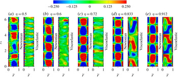
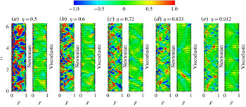
The curvature dependence of flow structure modification in viscoelastic TC flows is highlighted by the intriguing streamwise (azimuthal) vortices visualized in figures 2 and 3. Similar to our previous findings (Liu & Khomami Reference Liu and Khomami2013b
), for small
 $\unicode[STIX]{x1D702}$
values (
 ${<}0.72$
) the well-organized large-scale TV identified in Newtonian cases become unstable in the presence of polymer additives and break down into small-scale vortices, which are larger in size and fewer in number near the outer wall (see figures 2
a,b; 3
a,b). In the near-outer-wall region, the observed small-scale vortices are inertio-elastic Görtler vortices (IEGV) that arise due to the so-called IEGI (Liu & Khomami Reference Liu and Khomami2013b
). As shown below, the near-inner-wall vortices are generated mainly due to the elastic stresses and therefore are dubbed ‘elastic Görtler vortices’ (EGV). The increase in number of streamwise vortices for TC flow is usually commensurate with a drag (and torque) increase (Martińez-Arias et al.
Reference Martińez-Arias, Peixinho, Crumeyrolle and Mutabazi2014; Teng et al.
Reference Teng, Liu, Lu and Khomami2015). For the largest
 $\unicode[STIX]{x1D702}$
(of 0.912), the large-scale TV stack axially and occupy the entire gap, however, great differences in contour patterns of
 $\langle \unicode[STIX]{x1D714}_{\unicode[STIX]{x1D703}}\rangle _{\unicode[STIX]{x1D703},t}$
are observed between Newtonian and viscoelastic cases (see figure 2
e). These large-scale TV become more energetic and have their spanwise scales unaltered in the presence of polymer additives, as indicated in figure 4(a,b) by the highest spectral peaks at a wavenumber of
 $k_{z}=5$
which is the same for the Newtonian and viscoelastic cases. In terms of ensemble-averaged and instantaneous flow patterns (see figures 2 and 3), three main flow regimes are identified as: (1) small-scale GV only (
 $\unicode[STIX]{x1D702}=0.5$
), (2) co-existence of small-scale GV and large-scale TV (
 $\unicode[STIX]{x1D702}=0.72$
) and (3) large-scale TV only (
 $\unicode[STIX]{x1D702}=0.912$
). The appearance of vortical structures is qualitatively consistent with the prediction given by the extended PM criterion (Schäfer et al.
Reference Schäfer, Morozov and Wagner2018), i.e., increasing curvature
 $\unicode[STIX]{x1D716}$
(decreasing radius ratio
 $\unicode[STIX]{x1D702}$
) enhances purely elastic instability in TC flows.
Balance of angular momentum current across the gap for (a) Newtonian flow of
 $\unicode[STIX]{x1D702}=0.5$
and viscoelastic flows of (b)
 $\unicode[STIX]{x1D702}=0.5$
, (c)
 $\unicode[STIX]{x1D702}=0.6$
, (d)
 $\unicode[STIX]{x1D702}=0.72$
, (e)
 $\unicode[STIX]{x1D702}=0.833$
and (f)
 $\unicode[STIX]{x1D702}=0.912$
. Note that, the balance is similar for Newtonian flows of all
 $\unicode[STIX]{x1D702}$
considered, i.e.,
 $J_{c}^{\unicode[STIX]{x1D714}}$
is dominant in the bulk while
 $J_{d}^{\unicode[STIX]{x1D714}}$
in the wall regions.

For viscoelastic TC flows, the
 $\unicode[STIX]{x1D702}$
-dependent vortical structures underscore two coexisting DE mechanisms that could be interpreted separately in the following via the cases of
 $\unicode[STIX]{x1D702}=0.5$
and 0.912. First, the dramatic DE of the smallest
 $\unicode[STIX]{x1D702}$
has been ascribed to the occurrence of the small-scale GV near the inner and outer walls (Liu & Khomami Reference Liu and Khomami2013b
). These GV as shown in figures 2(a) and 3(a) enhance transverse momentum exchange and turbulent mixing of
 $\unicode[STIX]{x1D70F}_{r\unicode[STIX]{x1D703}}^{p}$
via their vortical circulations. Specifically, the fluid parcels with
 $\unicode[STIX]{x1D70F}_{r\unicode[STIX]{x1D703}}^{p}$
of much higher magnitude are carried from the near-inner-wall region to the bulk by the elastic Görtler vortices’ circulations and subsequently to the near-outer-wall region by the inertio-elastic Görtler vortices’ circulations, and vice versa. Consequently,
 $\langle \unicode[STIX]{x1D70F}_{r\unicode[STIX]{x1D703}}^{p}\rangle$
monotonically increases in the bulk (see figure 1
b) and has the most significant contribution to the angular momentum current away from the walls (see
 $J_{p}^{\unicode[STIX]{x1D714}}$
in figure 5
b, which is positive and thus a source term). In contrast, for the Newtonian case (see figure 5
a) the convective flux (
 $J_{c}^{\unicode[STIX]{x1D714}}$
) has the dominant contribution in the bulk whereas the diffusive flux (
 $J_{d}^{\unicode[STIX]{x1D714}}$
) is dominant in the wall regions. This situation is similar for Newtonian flows of all
 $\unicode[STIX]{x1D702}$
considered. This DE mechanism is clearly depicted in figure 6(a), where the viscoelastic TC flow with
 $\unicode[STIX]{x1D702}=0.5$
has positive
 $J_{r,z}^{\unicode[STIX]{x1D714}}$
values almost in the entire gap and the contour patterns are very reminiscent of those small-scale vortical structures shown in figures 2(a) and 3(a).
For the largest
 $\unicode[STIX]{x1D702}$
of 0.912, the DE mechanism originates from in the persistence of large-scale Taylor vortex circulations that facilitate a more efficient angular momentum transport, as evidenced by the following co-supportive facts. Specifically, the fluid parcels of high/low angular momentum are carried effectively by the intense outflows/inflows at the narrow boundaries of these Taylor vortex cells from the inner/outer to the outer/inner walls, before a comprehensive mixing occurs in the bulk (see figures 2
e and 3
e). This efficient angular momentum transport leads to a striking decrease/increase of angular momentum in the inner/outer wall regions, evinced by a positive
 $\langle u_{\unicode[STIX]{x1D703}}\rangle$
-gradient (reverse mean flow shear) that occurs in the bulk flow (see figure 1
a). Such a transverse transport is also applied to the polymer stress
 $\unicode[STIX]{x1D70F}_{r\unicode[STIX]{x1D703}}^{p}$
as indicated by figure 1(b). The most convincing evidence for this DE mechanism is provided in figure 5(f), which demonstrates that in the bulk
 $J_{c}^{\unicode[STIX]{x1D714}}$
has a positive contribution at
 $\unicode[STIX]{x1D702}=0.912$
that is even higher than
 $J^{\unicode[STIX]{x1D714}}$
and the negative
 $J_{p}^{\unicode[STIX]{x1D714}}$
acts as a sink term for the angular momentum. Also, the spectrum of the Reynolds stress (
 $\langle u_{r}^{\prime }u_{\unicode[STIX]{x1D703}}^{\prime }\rangle$
) has a higher polymer-induced basic peak at
 $k_{z}=5$
(see figure 4
b), pointing to the enhanced transverse momentum flux due to the large-scale TV. The well-organized axially stacked contour patterns of positive and negative
 $J_{r,z}^{\unicode[STIX]{x1D714}}$
shown in figure 6(e) for the viscoelastic TC flow present further evidence that these large-scale TV are the main driving force for the polymer-enhanced angular momentum transport.
Time and
 $\unicode[STIX]{x1D703}$
-direction averaged angular momentum current
 $J_{r,z}^{\unicode[STIX]{x1D714}}$
in (
 $r,z$
) plane for (a)
 $\unicode[STIX]{x1D702}=0.5$
, (b)
 $\unicode[STIX]{x1D702}=0.6$
, (c)
 $\unicode[STIX]{x1D702}=0.72$
, (d)
 $\unicode[STIX]{x1D702}=0.833$
and (e)
 $\unicode[STIX]{x1D702}=0.912$
, where
 $J_{r,z}^{\unicode[STIX]{x1D714}}=r^{3}\langle u_{r}\unicode[STIX]{x1D714}-\unicode[STIX]{x1D6FD}(\unicode[STIX]{x2202}\unicode[STIX]{x1D714}/\unicode[STIX]{x2202}r)/Re-(1-\unicode[STIX]{x1D6FD})(\unicode[STIX]{x1D70F}_{r\unicode[STIX]{x1D703}}^{p}/r)/Re\rangle _{\unicode[STIX]{x1D703},t}$
.

Considering the analogy between the turbulent TC flow and the turbulent RB convection (Eckhardt et al.
Reference Eckhardt, Grossmann and Lohse2007), the DE mechanism of
 $\unicode[STIX]{x1D702}=0.912$
has a physical origin akin to the polymer-enhanced heat transport in the bulk of turbulent RB convection. Specifically, the polymer-enhanced heat transport in turbulent RB convection is realized by enhancing the coherent heat fluxes related to thermal plumes and suppressing the incoherent heat fluxes related to small-scale turbulent fluctuations (Xie et al.
Reference Xie, Huang, Funfschilling, Li, Ni and Xia2015). Similarly, in viscoelastic TC flow at
 $\unicode[STIX]{x1D702}=0.912$
, DE is realized via enhancing the coherent angular momentum fluxes driven by the large-scale Taylor vortex circulations and weakening the incoherent transport by the small-scale GV (see figure 4
b). Further, the DE mechanism at
 $\unicode[STIX]{x1D702}=0.5$
can be ascribed to a polymer-induced enhancement of incoherent transport and homogenization of polymer stress,
 $\unicode[STIX]{x1D70F}_{r\unicode[STIX]{x1D703}}^{p}$
, by the small-scale GV.
The transition between the aforementioned DE mechanisms is clearly illustrated by detailed examination of figures 2, 3, 5 and 6. As shown in figures 2, 3 and 7, the viscoelastic TC flows present a striking transition in vortical structures with increasing
 $\unicode[STIX]{x1D702}$
; specifically this increase leads to weakening and elimination of the small-scale GV and the development and better organization (occupying the entire gap) of large-scale TV. The small-scale GV circulations evidently have a decreasing contribution to the angular momentum transport, while the contribution of large-scale TV to
 $J^{\unicode[STIX]{x1D714}}$
becomes more and more significant in the bulk (see
 $J_{p}^{\unicode[STIX]{x1D714}}$
,
 $J_{c}^{\unicode[STIX]{x1D714}}$
and
 $J^{\unicode[STIX]{x1D714}}$
in figure 5
b–f). An
 $\unicode[STIX]{x1D702}$
-dependent transition of contour patterns of
 $J_{r,z}^{\unicode[STIX]{x1D714}}$
which is consistent with the aforementioned vortical structures is clearly shown in figure 6. Note that the distorted large-scale TV appear at
 $\unicode[STIX]{x1D702}=0.833$
(see figures 2
d, 3
d and 6
d) where the smallest DE is observed in the present study. It should be caused by the weakening of small-scale GV (thus
 $J_{p}^{\unicode[STIX]{x1D714}}$
) and the enhancement in coherent transport of large-scale TV (thus
 $J_{c}^{\unicode[STIX]{x1D714}}$
). Although, the large-scale TV observed at
 $\unicode[STIX]{x1D702}=0.912$
are reminiscent of the secondary flow patterns driven by purely elastic instabilities as observed in Taylor–Dean flows (Joo & Shaqfeh Reference Joo and Shaqfeh1992) and serpentine channel flows (Zilz et al.
Reference Zilz, Poole, Alves, Bartolo, Levaché and Lindner2012); however, it is evident that these large-scale TV have a different driving mechanism due to the presence of significant inertial force.
Instantaneous vortical structures visualized by
 $Q$
-criterion with
 $Q=0.001$
and coloured by the distance to the inner wall for the three main regimes of viscoelastic TC flow. The flow structures in the region
 $\unicode[STIX]{x1D703}\in [3/2\unicode[STIX]{x03C0},2\unicode[STIX]{x03C0}]$
and
 $\tilde{r}\in [1/4,1]$
are not shown to clearly display the small-scale vortical structures near the inner wall.

Production terms of mean streamwise enstrophy (
 $\langle \unicode[STIX]{x1D714}_{\unicode[STIX]{x1D703}}\rangle ^{2}$
) near (a) the inner and (b) the outer wall for Newtonian and viscoelastic TC flows. Here,
 $S_{\unicode[STIX]{x1D714}}$
denotes the Newtonian production including the mean
 $[(\langle \unicode[STIX]{x1D74E}\rangle \boldsymbol{\cdot }\unicode[STIX]{x1D735}\langle \boldsymbol{u}\rangle \boldsymbol{\cdot }\langle \unicode[STIX]{x1D74E}\rangle )_{\unicode[STIX]{x1D703}}]$
and fluctuating
 $[(\langle \unicode[STIX]{x1D74E}^{\prime }\boldsymbol{\cdot }\unicode[STIX]{x1D735}\boldsymbol{u}^{\prime }\rangle \boldsymbol{\cdot }\langle \unicode[STIX]{x1D74E}\rangle )_{\unicode[STIX]{x1D703}}]$
strain stretch as well as the fluctuating enstrophy
 $[(\langle \boldsymbol{u}^{\prime }\unicode[STIX]{x1D74E}^{\prime }\rangle \boldsymbol{ : }\unicode[STIX]{x1D735}\langle \unicode[STIX]{x1D74E}\rangle )_{\unicode[STIX]{x1D703}}]$
, and
 $T_{\unicode[STIX]{x1D714}}$
represents the elastic production
 $[(1-\unicode[STIX]{x1D6FD})(\unicode[STIX]{x1D735}\times \langle \unicode[STIX]{x1D749}^{p}\rangle \boldsymbol{ : }\unicode[STIX]{x1D735}\langle \unicode[STIX]{x1D74E}\rangle )_{\unicode[STIX]{x1D703}}/Re]$
, where
 $\unicode[STIX]{x1D74E}=\unicode[STIX]{x1D735}\times \boldsymbol{u}$
. The insets show
 $S_{\unicode[STIX]{x1D714}}$
of the Newtonian cases. Here, plots are shown only for the three main regimes for clarity.

The mechanism that gives rise to the EGV is scrutinized by comparing the production terms of the balanced
 $\langle \unicode[STIX]{x1D714}_{\unicode[STIX]{x1D703}}\rangle ^{2}$
-budget equations (Kim et al.
Reference Kim, Li, Balachandar, Sureshkumar and Adrian2007) near the inner wall for the three main flow regimes. As seen in figure 8(a), the elastic production
 $T_{\unicode[STIX]{x1D714}}$
acts as the source term of increasing importance to the
 $\langle \unicode[STIX]{x1D714}_{\unicode[STIX]{x1D703}}\rangle ^{2}$
budgets versus the decreasing
 $\unicode[STIX]{x1D702}$
, and at
 $\unicode[STIX]{x1D702}=0.5$
overwhelms the contribution of
 $S_{\unicode[STIX]{x1D714}}$
that is the sole generation mechanism for streamwise vortical structures in the Newtonian TC flow. To this end, it is reasonable to describe the near-inner-wall small-scale vortices in viscoelastic cases of small
 $\unicode[STIX]{x1D702}$
, as EGV as they are reminiscent of those classical Newtonian GV (Wei et al.
Reference Wei, Kline, Lee and Woodruff1992). In contrast,
 $T_{\unicode[STIX]{x1D714}}$
and
 $S_{\unicode[STIX]{x1D714}}$
have comparable contributions in the outer wall region (see figure 8
b), where, consequently, the IEGV are generated (Liu & Khomami Reference Liu and Khomami2013b
). This is evidenced by the EGV and IEGV observed near the inner and outer walls, respectively, especially for
 $\unicode[STIX]{x1D702}=0.5$
(see figure 7
a).
4 Concluding remarks
In summary, a mechanism for curvature dependence of polymer-induced DE in TC flow has been proposed and substantiated for the first time via quantification of transverse angular momentum transport. Specifically, the drag enhancement is facilitated for small
 $\unicode[STIX]{x1D702}$
(large
 $\unicode[STIX]{x1D716}$
) by the small-scale GV that occur near the walls and result in much higher incoherent transport and homogenization of the polymer stress
 $\unicode[STIX]{x1D70F}_{r\unicode[STIX]{x1D703}}^{p}$
; and for large
 $\unicode[STIX]{x1D702}$
(small
 $\unicode[STIX]{x1D716}$
) by the large-scale TV that persist and account for much higher coherent angular momentum fluxes across the gap. The DE change as
 $\unicode[STIX]{x1D702}$
is increased is commensurate with a transition in vortical structures characterized by weakening and elimination of the small-scale GV and development and better organization (occupying the entire gap) of large-scale TV. Of particular interest is the viscoelastic TC flow with high curvature (small
 $\unicode[STIX]{x1D702}$
), where an enhanced elastic instability is observed as evinced by the excitation of small-scale streamwise vortices and a commensurate drastic enhancement of flow resistance. This suggests that elastic turbulence could be realized in TC flow by increasing the curvature over a certain critical value even at high inertia (
 $Re$
). To this end, this study has provided a viable road map for future research focused on the nature of localized elastic turbulence structures via coordinated experiments and DNS in curvilinear flows.
Acknowledgements
We are grateful to Dr Z. Wan and Dr J. Tang for many useful and illuminating discussions on the numerical results and the computational methods. This work was supported by the NSFC grant 91752110, 11621202, 11572312, Science Challenge Project (no. TZ2016001) and NSF grant CBET0755269.
Appendix A. Diffusivity independence check
The diffusivity independence check has been performed based on the case of
 $\unicode[STIX]{x1D702}=0.72$
, which is a typical regime with small-scale GV and large-scale TV coexisting. According to Sureshkumar et al. (Reference Sureshkumar, Beris and Avgousti1995, Reference Sureshkumar, Beris and Handler1997),
 $Sc$
should be as large as possible provided the numerical stability is maintained, and be increased linearly with the mesh size used. Therefore, test calculations have been performed for different
 $Sc$
values and mesh sizes. In the following, some representative results are presented to examine the diffusivity effects on the mean flow and turbulent motions of the viscoelastic case.
Comparison of typical results obtained for
 $\unicode[STIX]{x1D702}=0.72$
at different
 $Sc$
and mesh sizes: (a) mean azimuthal velocity
 $\langle u_{\unicode[STIX]{x1D703}}\rangle$
, (b) mean polymer stress component
 $\langle \unicode[STIX]{x1D70F}_{r\unicode[STIX]{x1D703}}^{p}\rangle$
, (c) root-mean-square (r.m.s.) values of three velocity components, and polymer stress component
 $\unicode[STIX]{x1D70F}_{r\unicode[STIX]{x1D703}}^{p}$
(d). The test calculations are performed with mesh size
 $128\times 256\times 256$
(in the
 $r\times \unicode[STIX]{x1D703}\times z$
directions) for
 $Sc=0.33$
and 0.42, and
 $256\times 512\times 512$
for
 $Sc=0.83$
.

As shown in figure 9(a,b), the profiles of
 $\langle u_{\unicode[STIX]{x1D703}}\rangle$
and
 $\langle \unicode[STIX]{x1D70F}_{r\unicode[STIX]{x1D703}}^{p}\rangle$
collapse well with each other, especially for the calculations of
 $Sc=0.42$
and 0.83. This indicates that using
 $Sc$
of the order of
 $O(10^{-1})$
can capture the main features of the velocity and polymer stress fields, as obtained by other high-
 $Re$
simulations (Sureshkumar et al.
Reference Sureshkumar, Beris and Avgousti1995, Reference Sureshkumar, Beris and Handler1997; Kim et al.
Reference Kim, Li, Balachandar, Sureshkumar and Adrian2007; Graham Reference Graham2014; Li et al.
Reference Li, Sureshkumar and Khomami2015; Zhu et al.
Reference Zhu, Schrobsdorf, Schneider and Xi2018; Lopez et al.
Reference Lopez, Choueiri and Hof2019). Furthermore, the turbulent statistics shown in figure 9(c,d) also present no qualitative modification for different
 $Sc$
. This is consistent with the previous findings as confirmed by Gupta & Vincenzi (Reference Gupta and Vincenzi2019) for viscoelastic flows of high
 $Re$
. To this point, our choice of
 $Sc=0.42$
and the corresponding mesh size is sufficient to resolve the global response and dynamical behaviour of turbulent TC flows of polymeric solutions considered.
Appendix B. Derivation of angular momentum current
For a fully developed turbulent viscoelastic TC flow, the same procedure used by Eckhardt et al. (Reference Eckhardt, Grossmann and Lohse2007) is applied to derive the formula of
 $J^{\unicode[STIX]{x1D714}}$
. First, taking the ensemble average over the azimuthal momentum (
 $u_{\unicode[STIX]{x1D703}}$
) equation of (2.2) yields
 $$\begin{eqnarray}0=\left\langle -u_{r}\frac{\unicode[STIX]{x2202}u_{\unicode[STIX]{x1D703}}}{\unicode[STIX]{x2202}r}-u_{\unicode[STIX]{x1D703}}\frac{\unicode[STIX]{x2202}u_{r}}{\unicode[STIX]{x2202}r}-\frac{2u_{r}u_{\unicode[STIX]{x1D703}}}{r}+\frac{\unicode[STIX]{x1D6FD}}{Re}\left[\frac{1}{r}\frac{\unicode[STIX]{x2202}}{\unicode[STIX]{x2202}r}\left(r\frac{\unicode[STIX]{x2202}u_{\unicode[STIX]{x1D703}}}{\unicode[STIX]{x2202}r}\right)-\frac{u_{\unicode[STIX]{x1D703}}}{r^{2}}\right]+\frac{1-\unicode[STIX]{x1D6FD}}{Re}\left(\frac{\unicode[STIX]{x2202}\unicode[STIX]{x1D70F}_{r\unicode[STIX]{x1D703}}^{p}}{\unicode[STIX]{x2202}r}+\frac{2\unicode[STIX]{x1D70F}_{r\unicode[STIX]{x1D703}}^{p}}{r}\right)\right\rangle .\end{eqnarray}$$
As the first three terms on the right-hand side of (B 1) sum to
 $r^{-2}\unicode[STIX]{x2202}_{r}(r^{2}u_{r}u_{\unicode[STIX]{x1D703}})$
, and the viscous and polymer stress terms can be written as
 $r$
-derivatives, we have
 $$\begin{eqnarray}0=\left\langle -\frac{1}{r^{2}}\left\{\frac{\unicode[STIX]{x2202}(r^{2}u_{r}u_{\unicode[STIX]{x1D703}})}{\unicode[STIX]{x2202}r}+\frac{\unicode[STIX]{x1D6FD}}{Re}\frac{\unicode[STIX]{x2202}}{\unicode[STIX]{x2202}r}\left[r^{3}\frac{\unicode[STIX]{x2202}(u_{\unicode[STIX]{x1D703}}/r)}{\unicode[STIX]{x2202}r}\right]+\frac{1-\unicode[STIX]{x1D6FD}}{Re}\frac{\unicode[STIX]{x2202}(r^{2}\unicode[STIX]{x1D70F}_{r\unicode[STIX]{x1D703}}^{p})}{\unicode[STIX]{x2202}r}\right\}\right\rangle .\end{eqnarray}$$
After multiplication by
 $r^{2}$
(which together with
 $\unicode[STIX]{x2202}/\unicode[STIX]{x2202}r$
commutate with
 $\langle \,\rangle$
) one obtains
 $$\begin{eqnarray}0=\frac{\unicode[STIX]{x2202}}{\unicode[STIX]{x2202}r}\left\{r^{3}\left[\langle u_{r}\unicode[STIX]{x1D714}\rangle -\frac{\unicode[STIX]{x1D6FD}}{Re}\frac{\unicode[STIX]{x2202}\langle \unicode[STIX]{x1D714}\rangle }{\unicode[STIX]{x2202}r}-\frac{1-\unicode[STIX]{x1D6FD}}{Re}\frac{\langle \unicode[STIX]{x1D70F}_{r\unicode[STIX]{x1D703}}^{p}\rangle }{r}\right]\right\}.\end{eqnarray}$$
Here, the angular velocity definition
 $\unicode[STIX]{x1D714}=u_{\unicode[STIX]{x1D703}}/r$
is considered. The conclusion is that the quantity
 $r^{3}[\cdots \,]$
must be independent of
 $r$
, i.e., it has the same value for any cylindrical surface at all
 $r$
with
 $R_{i}\leqslant r\leqslant R_{o}$
. In any event, it does not depend on
 $t$
,
 $\unicode[STIX]{x1D703}$
, or
 $z$
because of the averaging on these variables. Following Eckhardt et al. (Reference Eckhardt, Grossmann and Lohse2007), we interpret the constant
 $$\begin{eqnarray}J^{\unicode[STIX]{x1D714}}=r^{3}\left[\langle u_{r}\unicode[STIX]{x1D714}\rangle -\frac{\unicode[STIX]{x1D6FD}}{Re}\frac{\unicode[STIX]{x2202}\langle \unicode[STIX]{x1D714}\rangle }{\unicode[STIX]{x2202}r}-\frac{1-\unicode[STIX]{x1D6FD}}{Re}\frac{\langle \unicode[STIX]{x1D70F}_{r\unicode[STIX]{x1D703}}^{p}\rangle }{r}\right]\end{eqnarray}$$
as the conserved transverse current of azimuthal motion, transporting
 $\unicode[STIX]{x1D714}$
in the radial direction. The
 $J^{\unicode[STIX]{x1D714}}$
is rescaled as a quasi-Nusselt number
 $Nu_{\unicode[STIX]{x1D714}}$
by its Newtonian laminar value
 $J_{lam}^{\unicode[STIX]{x1D714}}$
as
 $Nu_{\unicode[STIX]{x1D714}}=J^{\unicode[STIX]{x1D714}}/J_{lam}^{\unicode[STIX]{x1D714}}$
(Eckhardt et al.
Reference Eckhardt, Grossmann and Lohse2007), where
 $J_{lam}^{\unicode[STIX]{x1D714}}$
is obtained based on the velocity profile of laminar flow as,
 $$\begin{eqnarray}J_{lam}^{\unicode[STIX]{x1D714}}=\frac{2}{Re}\frac{\unicode[STIX]{x1D6FA}R_{i}^{2}R_{o}^{2}}{R_{o}^{2}-R_{i}^{2}}.\end{eqnarray}$$