1. Introduction
Modelling selection falls within the most delicate problems in ecology and evolution. A variety of hypotheses have been proposed to describe how competing allelic types jostle against each other in trying to propagate successfully in the next generation [Reference Ewens25, Reference Gillespie28, Reference Kimura36, Reference Kimura and Ohta37]. Despite the complexity of the debate on the concept of selection itself, in population genetics there is agreement on the idea that an appropriate measure of the fitness strength of a given allelic type is related to the probability of its eventual fixation in the population. This agreement relies on the fact that generally, in population genetics models, fitness is considered as transitive in the sense that if in some conditions an allele 1 has a higher fitness than an allele 0 and an allele 2 has a higher fitness than an allele 1, then the allele 2 will have a higher fitness than the allele 0. This assumption impedes the modelling of non-transitive interactions, for instance the well-known rock–paper–scissors (RPS) interaction, where any of the three alleles involved may rise in frequency depending on the frequencies of the two other alleles present in the population [Reference Sinervo and Lively49].
Eco-evolutionary models aim to take into account feedback between ecological and evolutionary processes. In this setting, interactions are defined at the individual scale, which allows modelling of a much larger variety of interactions than in population genetics models (e.g. RPS interactions [Reference Billiard and Smadi6]). The drawback, however, is that the variation of population size makes the analysis more complex. For instance, even when studying processes faster than the time scale of population size evolution, we have to call upon technical results, such as large deviations results, to control the population size dynamics (see [Reference Champagnat13] for a classical example).
The aim of this paper is to construct a constant-size population model allowing us to consider very general interactions, as well as extreme reproductive events. This is achieved by a generalisation of a construction recently introduced in [Reference González Casanova and Spanò29], based on the concept of an ancestral selection graph introduced by Krone and Neuhauser [Reference Krone and Neuhauser39]. The main idea of this construction is that individuals first sample a random number of potential parents from the previous generation, and then choose their parent in the previous generation, with a rule which depends on the number and types of sampled potential parents. Mathematically, the rule that assigns types to the individuals, the colouring rule, is a family of random variables that take values in the type space and is indexed by the types of the potential parents. Note that the term ‘potential parents’ may be misleading, as in the current work we make it possible for an individual to have a type different from all of its potential parents; this is in order to model mutations. However, to make the link with [Reference González Casanova and Spanò29] clear, we have kept their notation. Following [Reference González Casanova and Spanò29], we also consider high-fecundity extreme reproductive events (
 $\Lambda$
-events), where one individual may give birth to a number of offspring of order N, the size of the population. After a proper rescaling of time, we derive a large population limit of our population model described by a generator, and which can be realised as the strong solution of a stochastic differential equation (SDE) under suitable conditions. This SDE generalises classical Wright–Fisher diffusion with selection and
 $\Lambda$
-Wright–Fisher processes to a multidimensional case with general frequency-dependent selection and jumps given by a
 $\Lambda$
-measure. We prove general properties on fixation and extinction for this class of models, and apply them to classical ecological interactions, such as RPS interactions or negative frequency-dependent selection.
Note that in a work conducted in parallel, Cordero, Hummel, and Schertzer [Reference Cordero, Hummel and Schertzer18] also considered a generalisation of [Reference González Casanova and Spanò29] to a general selection case. Their focus differs substantially from ours, as they consider the one-dimensional setting and concentrate on genealogies and duality properties of the frequency process with the ancestral process. Furthermore, they look for genealogies that minimise the number of potential ancestors. We encourage interested readers to have a look at [Reference Cordero, Hummel and Schertzer18] as well.
The paper is structured as follows. In Section 2 we describe the discrete model. Section 3 is dedicated to the derivation of the large population limit as well as the statement of general results on the processes under consideration. In Section 4 we present applications of our construction to model a set of ecological interactions, as well as properties of the long-time behaviour of these specific processes. Finally, the proofs are given in Section 5.
Here
 ${\mathbb{N}}^*\,:\!=\{1,2,\ldots,\}$
will denote the set of positive integers,
 ${\mathbb{N}}\,:\!= {\mathbb{N}}^* \cup \{0\}$
,
 ${\mathbb{Z}} \,:\!= -{\mathbb{N}}^* \cup {\mathbb{N}}$
, and for
 $N \in {\mathbb{N}}^*$
,
 $[N]\,:\!=\{1,2,\ldots,N\}$
. Finally,
 $|D|$
will denote the cardinality of a discrete set D, and for
 $K \in {\mathbb{N}}^*$
and
 $x \in [0, 1]^K $
,
 $\|x\|\,:\!= x_1+ \cdots +x_K$
.
2. The discrete model
We consider constant-size population models, with size
 $N \in {\mathbb{N}}^*$
, and with discrete non-overlapping generations. They generalise the models introduced in [Reference González Casanova and Spanò29]. The main novelty of our approach is that it includes the following features.
• We are in a multidimensional setting. We let
 $E= [K]$
denote the allelic type space, with
$K \in {\mathbb{N}}^*$
.
-
• To choose a real parent, knowing the set of potential parents, we will introduce a colouring rule, which may depend on N and on all the characteristics of the set of potential parents (number and frequencies of the different types), and may be random.
-
• The type of the newborn may not be a type carried by one of the potential parents. This allows us to take into account mutations, for instance.


Multitype models are widespread in the literature, both in population genetics (see e.g. [Reference Birkner, Blath, Mohle, Steinrucken and Tams7], [Reference Durrett and Mayberry22], [Reference Schweinsberg47], and [Reference Schweinsberg48], where even infinite type spaces are considered) and in eco-evolutionary models (e.g. [Reference Champagnat and Méléard14], [Reference Collet, Martínez, Méléard and San Martín17], [Reference Champagnat, Jabin and Méléard15], [Reference Bovier, Coquille and Neukirch9], and [Reference Bovier, Coquille and Smadi10]). There are also interesting instances of colouring (two-type) models in which individuals observe several potential parents and are coloured according to some rule depending on the observed sample [Reference Biswas, Etheridge and Klimek8, Reference Cordero, Hummel and Schertzer18, Reference González Casanova and Spanò29]. Questions regarding the existence and (lack of) uniqueness of a colouring rule that leads to a prescribed stochastic differential equation are addressed in [Reference Cordero, Hummel and Schertzer18]. The literature on mutations is vast [Reference Baake, Lenz and Wakolbinger3, Reference Durrett, Schmidt and Schweinsberg23, Reference Etheridge and Griffiths24]. However, as far as we are aware, the family of models introduced in this paper constitutes the first class that integrates all the above points, and luckily the flexibility of this family does not compromise its simplicity.
We begin in Section 2.1 with the description of births in generations without extreme reproductive events, and describe extreme reproductive events in Section 2.2. In Section 2.3 we introduce the multidimensional frequency process, which will be the process of interest in the rest of the paper.
2.1. Births without extreme reproductive events
Here
 $g \in {\mathbb{Z}}$
will always denote a generation. For
 $ N \in {\mathbb{N}}^*$
, we parametrise the strength of the selection via a probability distribution
 $Q_N$
on
 ${\mathbb{N}}^*$
. It will correspond to a number of ‘potential parents’ sampled by an individual. In order to describe the dynamics of our discrete model, we now introduce a graph and the concept of colouring rule.
Definition 2.1. Let
 $N\in{\mathbb{N}}^*$
and
 $V\,:\!={\mathbb{Z}}\times [N]$
. Consider a family of independent random variables uniformly distributed on [N],
 \begin{equation*}(U_{v,k}, v\in V, k\in{\mathbb{N}}^*){,}\end{equation*}
and a family of independent
 $Q_N$
distributed random variables,
 \begin{equation*}(K_v,v\in V){,}\end{equation*}
with values in
 ${\mathbb{N}}^*$
. Let
 $\mathcal{E}$
be the set of directed edges from an individual to its potential parents:
 \begin{equation*}\mathcal{E}=\{\{v,(g-1,U_{(v,k)})\}\text{ for all }v=(g,l)\in V\text{ such that } 1 \leq l \leq N \text{ and } k\leq K_v\}.\end{equation*}
The genealogical random digraph with parameters N and
 $Q_N$
is the random digraph
 $(V,\mathcal{E})$
.
For an individual v alive at generation g, the variables
 $(U_{v,k}, k \leq K_v)$
are thus the potential parents of v, alive at generation
 $g-1$
.
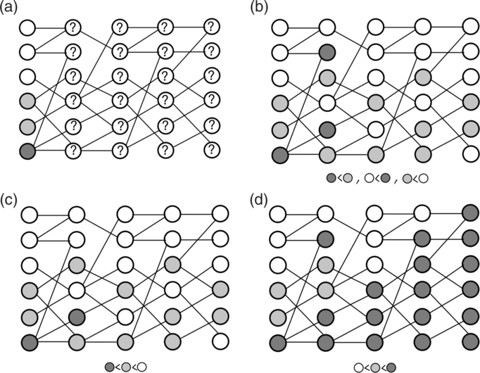
The idea of this graph is that we assign types to all the vertices in some generation, and we want to see types propagating in the subsequent generations. To do this we need to specify how a vertex is coloured (receive its type), given the types of the vertices in the previous generation which are connected to it. Figure 1 illustrates the following definition, which at first sight can seem technical.
After the random graph is generated (following the construction in [Reference González Casanova and Spanò29]) and the generation zero is arbitrarily coloured, i.e. the types of the individuals in that generation are determined, the colour/type of every individual in the subsequent generations is given inductively by a colouring rule. A colouring rule is a recipe for how to colour each individual depending on the types of its observed potential parents. For example, in (b), (c), and (d) we observe the same graph with the same colouring at generation zero. However, the colouring rule is different. Here, in all cases individuals copy their types from their potential parents and the colouring rule determines which colour to use if there are more than one option. We present two images with different transitive colouring rules (c, d) and one with the rock–paper–scissors colouring rule (b).

Definition 2.2. (Colouring rule.) Let
 \begin{equation*}\mathcal{C}=\bigcup_{n\in {\mathbb{N}}^*}E^n \end{equation*}
be the possible sets of potential parents with their type that can be sampled by an individual. An (N, E)-colouring rule is a family of probability distributions over E:
 \begin{equation*}C_N=\{c^N_{z}(\!\cdot\!)\}_{z \in \mathcal{C}}.\end{equation*}
The role of the distribution
 $c^N_{z}$
is to describe how an individual chooses its real parent and its type (if there is a mutation) when its set of potential parents is z and the population size is N.
To simplify the notation in some proofs, we will work under the assumption that, for any
 $z \in E$
,
 $ c^N_{z}= \delta_z. $
This condition ensures that if an individual samples only one potential parent, it is its real parent. We could omit this assumption but the notation would become cumbersome (but see Remark 3.1). Note also that we allow the colouring rule to depend on N, which leaves more freedom.
Definition 2.3. (Graph colouring without extreme events.) Fix
 $N\in{\mathbb{N}}^*$
,
 $Q_N$
a probability distribution on
 ${\mathbb{N}}^*$
, the space of types E, and an (N, E)-colouring rule
 $C_N$
. A colouring of the graph (V, E) is a function
 $f\colon V\rightarrow E$
. Let
 $V_g$
be the vertices in the gth generation. We construct a colouring f recursively by first arbitrarily defining f in
 $V_{0}$
and then extending the colouring to the subsequent generations using the colouring rule. Given that the colouring has been constructed in generation
 $g-1$
, for any
 $v\in V_g$
, let
 \begin{equation*} z_v=({\kern1.3pt}f(u_1),\ldots,f(u_{K_v}) ),\end{equation*}
where
 $u_k\in V_{g-1}$
is such that
 $(v,u_k)=(v,U_{v,k})$
for
 $k\leq K_v$
(in other words
 $u_k$
is a potential parent of v). For every type
 $i\in E,$
 \begin{equation*}{\mathbb{P}}({\kern1.3pt}f(v)=i)=c^N_{z_v}(i).\end{equation*}
We will use the terms type and colour interchangeably. Following the three previous definitions, the reproduction mechanism thus works as follows when there is no extreme reproductive event.
(1) (Choice of potential parents.) The individual v of generation g samples with replacement a number
$K_v$
distributed as
$Q_N$
of potential parents independently and uniformly distributed on
$(g-1) \times [N]$
,
$((g-1,U_{v,1}),\ldots,(g-1,U_{v,K_v}))$
.-
(2) (Choice of type.) The type of v is chosen according to the colouring rule, as described in Definition 2.3.



2.2. Births with extreme reproductive events
We now want to include the possibility of extreme reproductive events, that is to say events when one individual may generate a non-negligible fraction of the next generation. The motivation to consider such reproductive events comes from the observation that some species, in particular marine species [Reference Arnason2, Reference Hedgecock31] and most viruses [Reference Irwin, Laurent and Matuszewski33], have offspring distributions with very large variance, and that the Kingman coalescent is not a good model to describe their genealogy [Reference Hoscheit and Pybus32]. It is instead necessary to include the possibility of merging more than two individuals simultaneously. Such models have seen a growing interest since the discovery of
 $\Lambda$
-coalescent trees independently by Sagitov [Reference Sagitov46] and Donnelly and Kurtz [Reference Donnelly and Kurtz20], and their full description by Pitman [Reference Pitman45]. To this end, we introduce a random background formed by a sequence of independent and identically distributed (i.i.d.) Bernoulli trials,
 \begin{equation*} H = \{H_g \colon g \in {\mathbb{Z}}\} \in \{0, 1\}^\infty,\end{equation*}
with a probability of success
 $\gamma_N \in [0, 1]$
and a sequence
 \begin{equation*}Z = \{Z_g \colon g \in {\mathbb{Z}}\}\end{equation*}
of i.i.d. [0, 1]-valued random elements with common distribution
 $\Lambda$
. H and Z are assumed to be independent, and we also assume that
 $\Lambda([0, 1])<\infty$
. For every
 $g \in {\mathbb{Z}}$
,
 $H_g = 1$
(resp.
 $H_g = 0$
) indicates that at generation g extreme reproduction does (resp. does not) occur. Z will give the expected sizes of extreme reproductive events, when they occur. Let
 \begin{equation*}Y^* = \{Y^*_g\colon g \in {\mathbb{Z}}\}\end{equation*}
be a sequence of i.i.d. random variables, with
 $Y^*_{g}$
uniformly distributed among individuals in generation g and
 $Y^*$
independent of (H, Z). Conditionally on
 $Y^*_{g-1}$
, we thus assume that when
 $H_g=1$
, individuals in generation g choose one parent independently with the law
 \begin{equation*} \eta_g \,:\!= \mathcal{B}( Z_g ) \delta_{Y^*_{g-1}} + (1 - \mathcal{B} (Z_g)) U_g ,\end{equation*}
where
 $\mathcal{B}( Z_g )$
is distributed as a Bernoulli random variable with parameter
 $Z_g$
and
 $U_g$
is uniformly distributed on [N].
 $\mathcal{B}( Z_g )$
and
 $U_g$
are independent, and are drawn independently for each individual in generation g.
Definition 2.4. (Graph colouring with extreme events.) Fix
 $N\in{\mathbb{N}}^*$
,
 $Q_N$
a probability distribution on
 ${\mathbb{N}}^*$
, the space of types E, and a finite measure
 $\Lambda$
on [0, 1]. Given that the colouring has been constructed until generation
 $g-1$
, and that there is an extreme reproductive event at generation g, we have the following colouring for every type
 $i\in E$
and
 $v \in V_g$
:
 \begin{equation*}P({\kern1.3pt}f(v)=i\mid Z_g,Y_{g-1}^*)=Z_g \textbf{1}_{\{i, f(Y^*_{g-1})\}}+(1-Z_g) \frac{ \text{Card} \{ u \in V_{g-1}, f(u)=i \}}{N}.\end{equation*}
Following the previous definitions, the reproduction mechanism thus works as follows when there is an extreme reproductive event.
(1) (Choice of the individual with a large progeny.) An individual
$Y^*_{g-1}$
is drawn uniformly among individuals of the generation
$g-1$
. A variable
$Z_g$
is also drawn according to the distribution
$\Lambda$
. It will give the size of the extreme reproductive event.-
(2) (Choice to be part of the extreme event.) The individual v of generation g draws a Bernoulli variable
$\mathcal{B}_v(Z_g)$
with parameter
$Z_g$
. -
(3) If
$\mathcal{B}_v(Z_g)=1$
, the parent of v is
$Y^*_{g-1}$
. -
(4) If
$\mathcal{B}_v(Z_g)=0$
, the individual v chooses its parent uniformly in generation
$g-1$
.


2.3. Frequency processes
We have described in the two previous sections how individuals choose their parents in the previous generation. It allows us to construct a forward-in-time process, describing the dynamics of the composition of the population in terms of types. Fix
 $N\in{\mathbb{N}}^*$
,
 $Q_N$
a probability distribution on
 ${\mathbb{N}}^*$
,
 $\Lambda$
a finite measure on [0, 1],
 $\gamma_N \in [0,1]$
, and a colouring rule
 $C_N$
. Arbitrarily colour the graph at generation 0. Then colour generations
 $g \geq 1$
as follows.
• Colour the graph following Definition 2.3 with colouring rule
$C_N$
and distribution of the number of potential parents
$Q_N$
when there is no extreme reproductive event (
$H_g=0$
with probability
$1-\gamma_N$
).-
• Colour the graph following Definition 2.4 with Z
$\Lambda$
-distributed when there is an extreme reproductive event (
$H_g=1$
with probability
$\gamma_N$
).


Then the frequency process with parameters
 $(\Lambda, \gamma_N,Q_N,C_N)$
is by definition
 $\bar X^N_g\,{=}\,(X_g^{N,i}, i\,{\in}\,E)$
such that
 \begin{equation*}X^{N,i}_g=\frac{1}{N}|\{v\in V_{g}\colon f(v)=i\}|.\end{equation*}
This Markov chain describes the genetic composition of the population at any generation. The rest of the paper is devoted to the study of this process.
3. General results
The models and subsequent frequency processes we have just introduced allow us to consider very general interactions. Indeed we have total freedom on the colouring rule, and may even choose a type which is not carried by any of the potential parents sampled by an individual in the spirit of a mutation event.
In this section we will first present a rescaling of the population process, which generalises the class of Wright–Fisher processes considered until now. We will then describe the class of selection functions that we can obtain with our colouring rules, and we will finally prove general results on allele extinction and fixation of our class of models.
3.1. Large population limit
We will now prove that by rescaling time and taking the large population limit (
 $N \to \infty$
), we may obtain a time and space continuous process. We focus on the case
 \begin{equation*}1-Q_N(\{1\})=\!:\, \rho_N \to 0, \quad {N \to \infty},\end{equation*}
and to get a proper limit process we will rescale the time by a factor of order
 $\min\{\rho_N^{-1},N\}$
. For example, in the case
 $Q_N(\{1\})=1$
, we obtain the scale of the neutral Wright–Fisher model, and in the case
 $1-Q_N(\{1\})={\text{O}}(1/N)$
(corresponding to weak selection), the scale is the evolutionary scale N. If
 $1-Q_N(\{1\})={\text{O}}(1/N^b)$
for
 $b\in(0,1)$
(which corresponds to moderate selection) the scale is
 $N^b.$
Before stating our result we need to introduce the following notation, for any finite measure
 $\Lambda$
on [0, 1] and
 $\alpha \in (0,1/2)$
:
 \begin{equation} \hat \Lambda\,:\!= \frac{\Lambda}{\Lambda([0,1])}, \quad \Lambda^\alpha_N(z \in .) \,:\!= \frac{\Lambda(z \in .)}{z^2} \textbf{1}_{\{z \geq N^{-\alpha}\}},\quad \text{and}\quad \hat \Lambda^\alpha_N\,:\!= \frac{\Lambda^\alpha_N}{\Lambda^\alpha_N([0,1])}. \end{equation}
Let us also denote for
 $K \in {\mathbb{N}}^*$
the Kth simplex
 \begin{equation*} \Delta_K\,:\!= \{ x \in [0,1]^K, \|x\|\leq 1 \}. \end{equation*}
Moreover, for
 $N \in {\mathbb{N}}^*$
, given the colouring rule
 $C_N$
(recall Definition 2.1), consider the function
 $p^N\colon \Delta_K\to \Delta_K$
,
 $p^N=(p_1^N,\ldots,p_K^N)$
defined by
 \begin{equation} p_i^N(x)\,:\!={\mathbb{P}}({\kern1.3pt}f(v)=i\mid v \in V_1,X^N_0=x) \quad \text{{for all} } x \in \Delta_K,\ i \in E {,}\end{equation}
and
 $\mu^N\colon \Delta_K\rightarrow {\mathbb{R}}^K$
,
 $\mu^N=(\mu_1^N,\ldots,\mu_K^N)$
defined by
 \begin{equation} \mu_i^N(x)\,:\!=p_i^N(x)-x_i \quad \text{{for all} } x \in \Delta_K,\ i \in E. \end{equation}
Then we have the following convergence result.
Proposition 3.1. Let
 $\Lambda$
be a finite measure on (0, 1],
 $(C_N, N \in {\mathbb{N}})$
a sequence of colouring rules and
 $\alpha$
in
 $(0,1/2)$
. Consider for
 $N \in {\mathbb{N}}^*$
 $(\bar{X}_g^N, g \in {\mathbb{Z}})$
the frequency process with parameters
 $(\hat{\Lambda}^\alpha_N, \gamma_N,Q_N,C_N)$
. Assume that there exist
 $\kappa>0$
and
 $\sigma \geq 0$
such that:
(i)
$\lim_{N \to \infty} \rho_N^{-1} \mu^N_i(x)= \mu_i(x) \in {\mathbb{R}} $
for all
$ i \in E$
,
$x \in \Delta_K$
,-
(ii)
$\gamma_N = \Lambda^\alpha_N([0,1]) \rho_N/\kappa + o (\Lambda^\alpha_N([0,1]) \rho_N)$
, -
(iii)
$\lim_{N \to \infty} 1/(N\rho_N)= \sigma/\kappa<\infty$
and
$ \rho_N N^{2\alpha} \to 0$
, -
(iv) for
$k \geq 2$
,
$v \in V$
,
$\lim_{N \to \infty} Q_N(K_{v}=k\mid K_{v}>1)$
exists and is denoted by
$\pi_{k-1}$
, -
(v) for
$v \in V$
,
$\beta\,:\!= \lim_{N \to \infty} {\mathbb{E}} [K_{v}-1\mid K_{v}>1]= \sum_{k=1}^\infty k\pi_k<\infty$
.











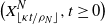
Then the sequence
 $\big(X^N_{\lfloor \kappa t /\rho_N \rfloor}, t \geq 0\big)$
is tight in the space of càdlàg functions
 $\mathbb{D}({\mathbb{R}}_+,[0,1])$
equipped with the Skorokhod topology. Further, if we let
 $\mathcal{A}^N$
denote the discrete generator of
 $X^N_{\lfloor \kappa t /\rho_N \rfloor}$
, the sequence of generators
 $\mathcal{A}^N$
, applied on
 $f \in \mathcal{C}_2(\Delta_K)\to {\mathbb{R}}$
and
 $x \in \Delta_K$
, converges to
 $\mathcal{A}$
given by
 \begin{align} \mathcal{A}f(x) &= \kappa \sum_{i=1}^K \mu_i(x) \frac{\partial f}{\partial x_i}(x) +\frac{\sigma}{2} \sum_{i,j=1}^K \sigma_{ij}(x) \frac{\partial^2 f}{\partial x_i x_j}(x) \notag \\*&\quad\, + \sum_{i=1}^K x_i \int_0^1 [{\kern1.3pt}f((1-z)x + z \textbf{e}_i)-f(x) ]\frac{\Lambda({\text{d}} z)}{z^2},\end{align}
where
 $\sigma_{ij}(x)=(1_{\{j=i\}}-x_j)x_i$
and
 $(\textbf{e}_i, 1 \leq i \leq K)$
is the canonical basis of
 ${\mathbb{R}}^K$
.
Assumption (iii) implies that
 $\min\{\rho_N^{-1},N\}={\text{O}}(\rho_N^{-1})$
. The case
 $\lim_{N \to \infty} 1/(N\rho_N)=\infty$
is the neutral case, and is well known in the literature. The first term of the generator describes a general frequency-dependent selective function, the second term is the classical Wright–Fisher diffusion, and the last part corresponds to the generator of a K-dimensional
 $\Lambda$
-Fleming–Viot process. Such a general multidimensional process including these three elements has not been introduced or studied until now, to the best of our knowledge. Extending this construction to include multiple simultaneous mergers would make the notation heavier and the proofs even more technical. For these reasons we do not include a
 $\Xi$
-coalescent part in this work.
Remark 3.1. Note that if we do not assume that when only one potential parent is sampled it is necessarily the real parent and its offspring inherits its type (see the end of Definition 2.2), we can obtain a different diffusion term. More precisely, if we introduce, for
 $i \in E$
and
 $x \in \Delta_K$
,
 \begin{equation*} g_i(x)\,:\!= \sum_{j=1}^K x_i c_j^N(i), \end{equation*}
and if G(x) is a random variable with values in
 ${\mathbb{N}}^K$
, and law given by
 \begin{equation*} {\mathbb{P}}(G(x)=Y)= \binom{N }{ Y_1,\ldots,Y_K}g_1^{Y_1}(x) \cdots g_K^{Y_K}(x), \end{equation*}
then for
 $(i,j) \in E^2$
and if the limit exists,
 \begin{equation*} \sigma \sigma_{ij}(x)= \lim_{N \to \infty} \frac{\kappa}{\rho_N} {\mathbb{E}} \biggl[ \biggl( \frac{G_i(x)}{N} -x_i\biggr) \biggl( \frac{G_j(x)}{N} -x_j\biggr) \biggr]. \end{equation*}
Under some assumptions on the parameters (see Corollary 3.1 for examples) we can link the infinitesimal generator
 $\mathcal{A}$
to the solutions to a stochastic differential equation (SDE) generalising the one-dimensional case derived in [Reference González Casanova and Spanò29].
Proposition 3.2. Assume that the following SDE is well-posed:
 \begin{align} {\text{d}} X(t) &= \mu(X(t))\,{\text{d}} t +\sqrt{\sigma}\zeta(X(t))\,{\text{d}} B_t \notag \\*
&\quad\, + \sum_{i=1}^{K} \textbf{e}_i \int_0^1 \int_0^1 z \Bigl( \textbf{1}_{\big\{ \sum_{j=1}^{i-1}X_j(t-\!) \leq u < \sum_{j=1}^{i}X_j(t-\!) \big\}}-X_i(t-\!) \Bigr) \tilde{N}({\text{d}} t, {\text{d}} u, {\text{d}} z),\end{align}
where B is a K-dimensional Brownian motion,
 $(\textbf{e}_i, i \leq K)$
is the canonical basis of E,
 $\tilde{N}$
is a compensated Poisson random measure on
 ${\mathbb{R}}_+ \times [0,1]\times [0,1]$
with intensity
 ${\text{d}} t {\text{d}} u \Lambda ({\text{d}} z)/z^2$
, and
 $\zeta$
has the following expression for
 $x \in \Delta_K$
:
 \begin{align*} \zeta_{ij}(x)&= 0 \quad \text{if } i<j,\\*\zeta_{ii}(x)&=\sqrt{ \frac{x_i(1-x_1- \cdots -x_i)}{1-x_1- \cdots -x_{i-1}} },\notag \\*\zeta_{ij}(x) &= -x_i \sqrt{ \frac{x_j}{(1-x_1 \cdots -x_{j-1})(1-x_1 \cdots -x_j)} } \quad \text{if } i >j .\end{align*}
If we aim to show the weak convergence of the sequence of frequency processes, we need to prove existence and uniqueness of the solution to the limiting SDE (3.5).
Theorem 3.1. Let us assume that the hypotheses of Proposition 3.1 hold and there exists a unique (in law) solution to (3.5) that we denote by
 $(X(t), t \geq 0)$
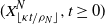
. Then the frequency process
 $(X^N_{\lfloor \kappa t /\rho_N \rfloor}, t \geq 0)$
converges in law to the space and time continuous process
 $(X(t), t \geq 0)$
, and
 $(X(t), t \geq 0)$
admits
 $\mathcal{A}$
defined in (3.4) as its infinitesimal generator.
To our knowledge, similar results have only been derived in the one-dimensional case in [Reference González Casanova and Spanò29] and recently in [Reference Cordero, Hummel and Schertzer18]. In this special case (where there are only two alleles) we can ensure the existence of a unique strong solution for the SDE under consideration. We can also provide this property in the multidimensional setting when specific assumptions are fulfilled. There have been a lot of recent developments in proving existence and uniqueness of multidimensional SDEs (see e.g. [Reference Barczy, Li and Pap5], [Reference Kurtz40], [Reference Kurtz41], [Reference Li and Pu42], and [Reference Xi and Zhu51]). It should be mentioned that moment duality is generally useful for proving such results, but we do not have this tool in the general setting that we are investigating. The next corollary presents some sufficient conditions.
Corollary 3.1. If the hypotheses of Proposition 3.1 hold, the function
 $\mu$
is continuous, and at least one of the following three statements is true:
(1)
$K=2$
,-
(2)
$\sigma \equiv 0$
and
$\int_0^{1}\Lambda({\text{d}} y)/y<\infty$
, -
(3) selection is transitive (see Section 4.1 below).


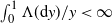
Then, using the notation of Theorem 3.1,
 \begin{equation*}\bigl(X^N_{\lfloor \kappa t /\rho_N \rfloor}, t \geq 0\bigr)\Rightarrow (X(t), t \geq 0),\end{equation*}
where
 $(X(t), t \geq 0)$
is the pathwise unique strong solution to the SDE (3.5) and admits
 $\mathcal{A}$
defined in (3.4) as its infinitesimal generator.
The assumption
 $\sigma \equiv 0$
in statement (2) of the above result comes from the fact that the diffusion coefficient of (3.5) is not Lipschitz on
 $\Delta_K$
if
 $\sigma>0$
. However, as long as the solution to (3.5) is not too close to the boundaries of
 $\Delta_K$
, this problem does not arise. Hence, if we introduce the stopping times, for any
 $0<\varepsilon<1/2$
,
 \begin{equation*} T_{(\varepsilon,X)}\,:\!= \inf \Bigl\{ t \geq 0, \min_{1 \leq i \leq K} X_i(t)\leq \varepsilon \Bigr\}, \end{equation*}
we can prove the following result.
Lemma 3.1. Let
 $0<\varepsilon<1/2$
and assume that
 \begin{equation*}\int_0^1 \Lambda({\text{d}} y)/y<\infty.\end{equation*}
Then the SDE (3.5) admits a pathwise unique strong solution X on the time interval
 $[0,T_{(\varepsilon,X)})$
.
3.2. Selection functions
This section generalises the ideas of [Reference Cordero, Hummel and Schertzer18] to the multidimensional setting. As we have a large degree of freedom in the choice of the colouring rule, the class of selection functions we can obtain with this construction is very general. It is the content of the next lemma.
Lemma 3.2. Let
 $N \in {\mathbb{N}}^*$
,
 $\kappa >0$
, and
 $\mu\colon \Delta_K\rightarrow {\mathbb{R}}^K$
be a continuous function such that there exists
 $\lambda>0$
, with the property that
 \begin{equation*}g(x)\,:\!=\frac{\kappa\mu( x)}{\lambda}+x \in \Delta_K \quad \text{{for all} } x \in \Delta_K. \end{equation*}
Assume also that there is a unique (in law) solution to (3.5). Then there exists a sequence of couples of distribution and colouring rule
 $(Q_N,C_N)$
such that the sequence of frequency processes
 $X^N_{\lfloor \kappa t /\rho_N \rfloor}$
converges to
 $(X(t), t \geq 0)$
, which has infinitesimal generator
 $\mathcal{A}$
given by (3.4).
The above lemma does not provide a colouring rule independent of N leading to
 $\mu$
as a limit selection function. This is done in the next lemma, but with a less general class of functions.
Lemma 3.3. Let
 $\kappa >0$
,
 $n \in {\mathbb{N}}$
, and
 $\mu\colon \Delta_K\rightarrow {\mathbb{R}}^K$
be a continuous function such that there exists
 $\lambda>0$
, with the property that
 \begin{equation*}g(x)\,:\!=\frac{\kappa\mu(x)}{\lambda}+x\in \Delta_K \quad {{for\ all} }\ x \in \Delta_K, \end{equation*}
and g is a polynomial function of degree n. For each
 $i\in E$
, let
 \begin{equation*}g_i( x)=\sum_{z=(z_1,\ldots,z_K)}\binom{n}{z}\alpha^i_{ z}\prod_{r=1}^Kx_r^{z_r}\end{equation*}
be the representation of
 $g_i$
in the Bernstein basis. Then the choices
 \begin{equation*}Q_N=(1-\rho_N)\delta_1+\rho_N\delta_n\end{equation*}
and
 \begin{equation*}c^N_{ z}(i)=\alpha^i_{ z}\end{equation*}
for every N-dimensional vector z and
 $c^N_{ z}=\delta_{ z}$
for every one-dimensional vector z lead to the same conclusions as in the previous lemma.
3.3. On allele extinction and fixation
The end of Section 3 deals with extinction and fixation properties of the frequency process
 $(X(t), t \geq 0)$
. We first provide a sufficient condition for one of the alleles to reach fixation in a finite time.
Before stating it, we introduce a parameter that depends on the mean number of potential parents
 $\beta$
(defined in Proposition 3.1) and on the measure
 $\Lambda$
:
 \begin{equation} \kappa^* \,:\!=\frac{1}{\beta}\int_0^1\log(1-y)\frac{\Lambda({\text{d}} y)}{y^2}.\end{equation}
Proposition 3.3. Assume that there are no mutations (the offspring inherits the type of one of the potential parents) and the infinitesimal generator of the frequency process
 $(X(t), t \geq 0)$
is given by (3.4). Then there is almost sure fixation of one of the alleles in finite time if at least one of the two following conditions is satisfied:
(i)
$\sigma>0$
,-
(ii)
$\kappa < \kappa^* <\infty$
.


Remark 3.2. Following Definitions 2.1 and 2.3, the assumption ‘there are no mutations’ can be written rigorously:
 \begin{equation*} {\mathbb{P}}({\kern1.3pt}f(v)=i)=0 \quad \text{if $ f(U_{v,k})\neq i $ for all (\textit{v},\textit{g},\textit{k}) such that $ \{ v,(g-1,U_{v,k}) \} \in \mathcal{E}$.} \end{equation*}
We end this section with a result on the way alleles become extinct in the case of a Wright–Fisher diffusion (without jumps). This is an extension of a recent result by Coron and co-authors, who proved this result in the neutral case [Reference Coron, Méléard and Villemonais19].
Proposition 3.4. Assume that the SDE (3.5) is well-posed and let
 $(X(t), t \geq 0)$
denote a solution. Suppose that
 $\Lambda\equiv0$
,
 $\sigma>0$
and that
 $\mu$
satisfies
 \begin{equation*} \mu_i(x) = x_i (1-x_i) s_i(x) \quad {for\ all} \ x \in \Delta_K {,} \end{equation*}
where
 $s=(s_1,\ldots,s_K)$
is a continuous function on
 $\Delta_K$
. Then one of the alleles ultimately fixates, and before its fixation, the population experiences successive (and non-simultaneous) allele extinctions.
Remark 3.3. Note that as soon as we require that the type of each individual is among the types of its potential parents (no mutations),
 $\mu_i(x)$
will be of the form
 $\mu_i(x)=x_i \tilde{s}_i(x) $
, with
 $\tilde{s}$
bounded. Indeed, by definition, for
 $i \in E$
,
 $N \in {\mathbb{N}}^*$
, and
 $x \in \Delta_K$
,
 \begin{equation*} \mu_i^N(x)= (Q_N(1)-1)x_i + \sum_{k=2}^\infty Q_N(k) {\mathbb{P}}({\kern1.3pt}f(v)=i\mid v \in V_1,X_0^N=x,K_v=k). \end{equation*}
However, as a type i individual has to be sampled among the potential parents for v to be of type i, we get
 \begin{equation*} {\mathbb{P}}({\kern1.3pt}f(v)=i \mid v \in V_1,X_0^N=x,K_v=k)\leq 1 - (1-x_i)^k = x_i ( 1+ (1-x_i)+ \cdots + (1-x_i)^{k-1} ). \end{equation*}
Hence, in the absence of mutation, to check the conditions of Proposition 3.4 on
 $\mu$
we will just have to prove that
 $\mu_i(x)/(1-x_i)$
is bounded.
The next section is dedicated to examples of selection functions we can consider with our models. All of them satisfy the assumption of Proposition 3.4.


4. Applications
In this section we illustrate the generality of our construction by using it to model various ecological interactions. When the calculations are not too cumbersome, we also provide the selective function obtained as a limit.
4.1. Transitive ordering
This is the classical assumption in population genetics models, consisting in ordering transitively the fitness of the different alleles. In this scheme, 1 has a smaller fitness than
 $\{2,\ldots,K\}$
, 2 has a larger fitness than 1, but a smaller fitness than
 $\{3,\ldots,K\}$
, and so on. Thus the colouring rule consists in taking one parent among the potential parents with the highest type,
 $c_z(\!\cdot\!)=\delta_{\sup_z}$
, where
 $\sup_z$
is the supreme norm of the vector
 $z \in E$
.
If we consider only two alleles and that the number of potential parents is one or two, we find as a limit the classical Wright–Fisher process with selection (plus jumps), where the frequency
 $(Y_t, t \geq 0)$
of type 1 individuals is the unique strong solution to
 \begin{equation*} {\text{d}} Y_t = -\kappa Y_t(1-Y_t)\,{\text{d}} t+ \sqrt{\sigma Y_t(1-Y_t)}\,{\text{d}} W_t+ \int_0^1 \int_0^1 y ( \textbf{1}_{\{u < Y_{t-} \}}-Y_{t-} ) \skew3\tilde{M}({\text{d}} t, {\text{d}} u, {\text{d}} z) \end{equation*}
where
 $\skew3\tilde{M}$
is a compensated Poisson measure with intensity
 $ {\text{d}} t {\text{d}} u \Lambda ({\text{d}} z)/z^2 $
. If we allow the number of potential parents to exceed two, but still with only two alleles, it amounts to the model described and studied in [Reference González Casanova and Spanò29], where the selective function is
 \begin{equation} \mu_1(x)=\mu_1(x_1,1-x_1)= \sum_{k=1}^\infty \pi_k \big( x_1^{k+1}-x_1 \big) ,\end{equation}
where we recall that
 $\pi$
was introduced in Proposition 3.1.
Finally, if we consider a finite number of alleles larger than two, we obtain the following selective function for
 $i \in E$
:
 \begin{equation} \mu_i(x) = \sum_{k=1}^\infty \pi_k ((x_0+ \cdots +x_i)^{k+1}-(x_0+ \cdots +x_{i-1})^{k+1}-x_i).\end{equation}
This can be deduced from (4.1). Indeed, for any
 $i \in E$
, if we divide the alleles into two groups, 1 to i and
 $i+1$
to K, the relative frequencies of the two groups evolve as if there were only two types in the population. Doing the same with the groups 1 to
 $i+1$
and
 $i+2$
to K, and so on, allows us to conclude.
By extending results in [Reference González Casanova and Spanò29] we can provide the probability of fixation of the different alleles. In [Reference González Casanova and Spanò29] the authors prove moment duality between the frequency process of the weakest allele and a process
 $(D_t, t \geq 0)$
named the ancestral process and corresponding to the limit of the number of potential ancestors of a sample taken at a given generation. The ancestral process has the following generator:
 \begin{align} Lf(n)& = \kappa \sum_{i=2}^\infty \pi_i [{\kern1.3pt}f(n+i-1)-f(n)]+ \sigma \binom{n}{ 2} [{\kern1.3pt}f(n-1)-f(n)] \notag \\* &\quad\, + \sum_{k=2}^n \binom{n }{ k} \lambda_{nk}[{\kern1.3pt}f(n-k+1)-f(n)],\end{align}
for every
 $n \in {\mathbb{N}}$
and
 $f\colon {\mathbb{N}} \to {\mathbb{R}}$
twice continuously differentiable, where we recall that
 $\pi$
was defined in Proposition 3.1, and for
 $2 \leq k \leq n$
,
 $\lambda_{nk}$
is given by
 \begin{equation*} \lambda_{nk}= \int_0^1 y^k (1-y)^{n-k} \frac{\Lambda({\text{d}} y)}{y^2}. \end{equation*}
It appears that the behaviour of
 $(D_t, t \geq 0)$
provides the long-time equilibrium of the frequency process
 $(X(t), t \geq 0)$
. Recall the definition of
 $\kappa^*$
in (3.6). Then we have the two following possible long-time behaviours.
Lemma 4.1. Let us assume that the hypotheses of Proposition 3.1 are satisfied and that
 $\mu$
is given by (4.2). Let X denote the process with generator
 $\mathcal{A}$
defined in (3.4).
(i) If
$\kappa < \kappa^*<\infty$
,
$(D_t, t \geq 0)$
has a unique stationary distribution
$\nu$
, and for
$i \in E$
and
$x \in \Delta_K$
,
where
\begin{equation*} {\mathbb{P}}_x\Bigl(\lim_{t \to \infty}X_i(t)=1\Bigr)= \phi_\nu(x_0+ \cdots +x_i)-\phi_\nu(x_0+ \cdots +x_{i-1}), \end{equation*}
$\phi_\nu$
is the probability generating function of
$\nu$
.
-
(ii) If
$\kappa \geq \kappa^*$
, and if we let S denote the maximal label of alleles present at the beginning,
we get
\begin{equation*} S\,:\!= \sup \{ i \in E, x_i>0\}, \end{equation*}
\begin{equation*} {\mathbb{P}}_x\Bigl(\lim_{t \to \infty}X_S(t)=1\Bigr)=1. \end{equation*}


This result says that if the selection function is not strong enough (
 $\kappa$
small) or if the variance generated by the choice of parents in the previous generation (
 $\sigma>0$
) or extreme reproductive events is large enough, the latter can override the selection, and a deleterious allele may fixate.
Remark 4.1. In the case of transitive fitness (
 $\mu$
given by (4.2)), we could consider more general extreme reproductive events (more precisely
 $\Xi$
reproductive events: see [Reference González Casanova and Spanò29]). We would still obtain the statement (3) of Corollary 3.1 and Lemma 4.1. We do not provide details here, for the sake of readability.
Remark 4.2. The classical moment duality method that we used here cannot be applied if the colouring rule is not transitive. However, the notion of ancestry can still be useful in more general frameworks, as we will see below.
4.2. Transitive ordering with mutations
We can still consider that the highest type is the best when choosing among potential parents, but add mutations with some probability. As a consequence, the offspring can carry a type different from the types of all of its potential parents. Note that this colouring rule is not deterministic. The form of the mutation probability may depend on what we want to model (e.g. Muller’s ratchet, or fixation of a beneficial mutant).
4.3. Logistic competition
We want to model competitive interactions, which can depend on the types of the competing individuals. These kinds of competitive interactions have been widely studied by ecologists and in the setting of varying-size stochastic population models, as they allow us to model, for instance, the preference for different types of resources or spaces depending on the individual’s type, and lead to non-monotonic dynamics (see e.g. [Reference Méléard and Tran43] or [Reference Champagnat and Méléard14]). To model these interactions, we assume that
 $K_v$
is only supported on
 $\{1,2\}$
, and that the assumptions of Proposition 3.1 are satisfied. When
 $K_v=1$
the real parent is the potential parent sampled uniformly at random in the previous generation by v. When
 $K_v=2$
and the two potential parents have the same type, the real parent is chosen among them with probability
 $1/2$
for each. Now assume that they have different types, which we denote by i and j. Then the potential parent of type i transmits its type with probability
 $p_{ij}$
, and the potential parent of type j transmits its type with probability
 $p_{ji}$
, with
 $p_{ij}+p_{ji}=1$
. We thus get
 \begin{align} \mu_i( x)&= x_i^2+2x_i\sum_{j \neq i} p_{ij}x_j -x_i \notag \\*&= x_i\biggl[x_i+2\sum_{j \neq i} (1-p_{ji})x_j -1\biggr] \notag \\&= x_i\biggl[x_i+2(1-x_i)-2\sum_{j \neq i} p_{ji}x_j -1\biggr] \notag \\*&= x_i\biggl[1-x_i-2\sum_{j \neq i} p_{ji}x_j \biggr].\end{align}
We thus obtain a competitive Lotka–Volterra function, whose competition coefficients are functions of probabilities
 $p_{ij}$
. Note that the intracompetition coefficient (1 here) is constrained by the fact that the frequency of type i cannot exceed 1, and equals 1 when the population is monomorphic.
4.4. Rock–paper–scissors
RPS is a children’s game where rock beats scissors, which beat paper, which in turn beats rock. Such competitive interactions between morphs or species in nature can lead to cyclical dynamics, and have been documented in various ecological systems [Reference Buss and Jackson11, Reference Cameron, White and Antonovics12, Reference Kerr, Riley, Feldman and Bohannan35, Reference Kirkup and Riley38, Reference Nahum, Harding and Kerr44, Reference Sinervo and Lively49, Reference Taylor and Aarssen50]. Let us describe two examples of such cycles. The first one [Reference Sinervo and Lively49] is concerned with patterns of sexual selection in some male lizards. Males are associated to their throat colours, which have three morphs. Type 1 individuals (orange throat) are polygamous and very aggressive. They control a large territory. Type 2 individuals (dark-blue throat) are monogamous. They control a smaller territory. Finally type 3 individuals (prominent yellow stripes on the throat, similar to receptive females) do not engage in female-guarding behaviour but roam around in search of sneaky matings. As a consequence of these different strategies, type 1 outcompetes type 2 (because males are more aggressive), which outcompetes type 3 (as males of type 2 are able to control their small territory and guard their female), which in turn outcompetes type 1 (as males of type 1 are not very efficient in defending their territory, having to split their efforts between several females). The second example [Reference Kirkup and Riley38] is concerned with the interactions between three strains of Escherichia coli bacteria. Type 1 individuals release toxic colicin and produce an immunity protein. Type 2 individuals produce the immunity protein only. Type 3 individuals produce neither toxin nor immunity. Then type 1 is defeated by type 2 (because of the cost of toxic colicin production), which is defeated by type 3 (because of the cost of immunity protein production), which in turn is defeated by type 1 (not protected against toxic colicin).
To model such interactions in our setting, we assume as in the previous example that
 $K_v$
is supported on
 $\{1,2\}$
, and we introduce the partial order
 $1<2$
,
 $2<3$
,
 $3<1$
. When two potential parents with different types are sampled as potential parents, they compete and the ‘strongest’ transmits its type. We thus define the colouring rule
 $c^N_z(\!\cdot\!) = \delta_{\max \{z_1,z_2\}}$
, and obtain as limit the selective function, for
 $i \in E$
and
 $x \in \Delta_K$
,
 \begin{equation} \mu_i(x)=\kappa x_i (x_{\text{mod}_3(i-1)}-x_{\text{mod}_3(i+1)}),\end{equation}
where
 $\text{mod}_3(i)$
is the rest of the division of i by 3.
The next result tells us that either there is fixation in the RPS selection case, or at least the product of allele frequencies approaches 0 when time increases.
Lemma 4.2. Let us consider the process
 $(X(t), t \geq 0)$
with infinitesimal generator
 $\mathcal{A}$
defined in (3.4) and
 $\mu$
given by (4.5), that is to say the RPS selection. Then
 \begin{equation*}{\mathbb{E}}[\ln (X_1(t) X_2(t) X_3(t))] \searrow -\infty, \quad t \to \infty\end{equation*}
if and only if
 $\sigma\neq 0$
or
 $\Lambda\neq 0$
.
Remark 4.3. Note that if
 $\sigma$
and
 $\kappa$
satisfy the assumptions of Proposition 3.3, we know that one of the three alleles gets fixed in finite time.
4.5. Food web
The previous example can be generalised to any number of types and any partial order. In particular, it is well suited to representing food webs. A possibility could be that
 $i<j$
indicates that i is eaten by j, and if i and j do not eat each other,
 $i=j$
would indicate that we take
 $p_{ij}=p_{ji}=1/2$
in the example of logistic competition.
4.6. Negative frequency-dependent selection
Negative frequency-dependent selection is a common form of selection in nature. It refers to the fact that it is more advantageous for an individual to be of a type in the minority in the population. In the case of the orchid Dactylorhiza sambucina, for instance, there is a negative frequency-dependent selection on colours due to behavioural responses of pollinators to lack of reward availability [Reference Gigord, Macnair and Smithson27]. In other populations, such a selection can be due to the fact that some predators concentrate on common varieties of prey and overlook rare ones [Reference Allen1].
To represent this form of selection, we sample
 $K_v$
potential parents as usual, and choose the real parent uniformly at random among the potential parents with the less frequent type. If there are several ‘less frequent types’ we choose one of them uniformly at random. Note that to represent such a form of selection, it is necessary to sample more than two potential parents with positive probability. Otherwise it would result in no selection (
 $\mu\equiv 0$
). For the sake of simplicity, to compute
 $\mu$
we will assume that
 $K_v$
is supported on
 $\{1,3\}$
, but we could consider any distribution for
 $K_v$
. In this case, if there are three potential parents, for a type i parent to be chosen there are three possibilities. Either all the potential parents are of type i, or only one parent is of type i and the two other parents are of type j different from i, or the three parents are of different types, i, j, and k. Summing the probabilities of these three events, we get
 \begin{align} \notag \mu_i(x)&= \biggl[x_i^3 + 3 x_i \biggl(\sum_{j \neq i} x_j^2 + \frac{1}{3} \sum_{j \neq k, j,k \neq i}x_jx_k\biggr)-x_i \biggr]\\*&= x_i\biggl[x_i^2-1 + 3 \biggl( \frac{2}{3} \sum_{j \neq i} x_j^2 + \frac{1}{3}(1-x_i)^2\biggr) \biggr] \notag \\*&=2 x_i\biggl[ \sum_{j \neq i} x_j^2-x_i(1-x_i) \biggr].\end{align}
4.7. Positive frequency-dependent selection
Positive frequency-dependent selection refers to the fact that it is more advantageous for an individual to be of a type in the majority in the population. This is for instance the case for warning signals in butterflies, indicating that one individual is poisonous for predators [Reference Chouteau, Arias and Joron16]. The modelling of this type of selection is similar in spirit to the previous one. Among the potential parents, we choose uniformly a parent with the most frequent type. If there are several ‘most frequent types’ we choose one of them uniformly at random. For an easy computation, we make the same assumptions on
 $K_v$
as in the previous example. In this case, if there are three potential parents, for a type i parent to be chosen there are three possibilities. Either all the potential parents are of type i, or two parents are of type i and the other one is of type j different from i, or the three parents are of different types, i, j, and k. Summing the probabilities of these three events, we get
 \begin{align} \mu_i( x)= x_i\biggl[x_i^2-1 + 3 x_i (1-x_i) + \sum_{j \neq k, j,k \neq i}x_jx_k \biggr]= x_i\biggl[(2x_i-1)(1-x_i) + \sum_{j \neq k, j,k \neq i}x_jx_k \biggr].\end{align}
The remainder of the paper is dedicated to the proofs.
5. Proofs
5.1. Proofs for Section 3
Before focusing on the convergence of the frequency process, we will first prove Proposition 3.2, which states that the infinitesimal generator
 $\mathcal{A}$
defined in (3.4) characterises the solution to (3.5) when this equation is well-posed.
Proof of Proposition 3.2. We will show that
 $\mathcal{A}$
is the infinitesimal generator of the process
 $(X(t), t\geq 0)$
. The drift part (with the selection function
 $\mu$
) is straightforward, and the last part is the classical generator of a
 $\Lambda$
-Fleming–Viot process (see e.g. [Reference Griffiths30]). Let us check that the diffusive part has the good form. For
 $i<j \in E^2$
, from (3.5) and Itô’s formula, we have
 \begin{align*} \frac{{\text{d}} \langle X_i,X_i \rangle}{{\text{d}} t} & = \sigma \sum_{k=1}^i \zeta_{ik}^2 (X)\\* & = \sigma\zeta_{ii}^2(X)+ \sigma\sum_{k=1}^{i-1} \zeta_{ik}^2 (X)\displaybreak\\& = \sigma \frac{X_i(1-X_1- \cdots -X_i)}{1-X_1- \cdots -X_{i-1}} + \sigma X_i^2 \sum_{k=1}^{i-1}\frac{X_k}{(1-X_1 \cdots -X_{k-1})(1-X_1 \cdots -X_k)}\\& = \sigma \frac{X_i(1-X_1- \cdots -X_i)}{1-X_1- \cdots -X_{i-1}} + \sigma X_i^2 \sum_{k=1}^{i-1}\biggl( \frac{1}{1-X_1 \cdots -X_{k}} - \frac{1}{1-X_1 \cdots -X_{k-1}}\biggr)\\& = \sigma \frac{X_i(1-X_1- \cdots -X_i)}{1-X_1- \cdots -X_{i-1}} + \sigma X_i^2 \biggl( \frac{1}{1-X_1 \cdots -X_{i-1}} - 1\biggr)\\& = \sigma \frac{X_i}{1-X_1- \cdots -X_{i-1}}( (1-X_1- \cdots -X_i) + X_i-X_i(1-X_1 \cdots -X_{i-1}))\\*& = \sigma X_i(1-X_i),\end{align*}
and
 \begin{align*} \frac{{\text{d}} \langle X_i,X_j \rangle}{{\text{d}} t} & = \sigma \sum_{k=1}^i \zeta_{ik} (X) \zeta_{jk} (X)\\* &=\sigma \zeta_{ii}(X)\zeta_{ji}(X)+ \sigma \sum_{k=1}^{i-1} \zeta_{ik} (X) \zeta_{jk} (X)\\& = -\sigma\sqrt{ \frac{X_i(1-X_1- \cdots -X_i)}{1-X_1- \cdots -X_{i-1}} }X_j \sqrt{ \frac{X_i}{(1-X_1 \cdots -X_{i-1})(1-X_1 \cdots -X_i)} } \\*& \quad\, + \sigma X_i X_j \sum_{k=1}^{i-1}\frac{X_k}{(1-X_1 \cdots -X_{k-1})(1-X_1 \cdots -X_k)}\\& = -\sigma\frac{X_i X_j}{1-X_1- \cdots -X_{i-1}} + \sigma X_i X_j \biggl( \frac{1}{1-X_1 \cdots -X_{i-1}} - 1\biggr)\\*& = - \sigma X_i X_j.\end{align*}
Proof of Theorem 3.1. Under the assumption of existence and uniqueness of the solution of (3.5), it is enough to prove the
 $L_1$
-convergence of the sequence of generators of
 $(X_{\lfloor M_t^N\rfloor}^N, t \geq 0)$
, where
 $M^N$
is a Poisson process with rate
 $\kappa / \rho_N$
, to the generator of
 $(X(t), t \geq 0)$
, evaluated in the
 $C_2$
functions
 $[0,1]\mapsto{\mathbb{R}}$
(see [Reference Kallenberg34, Lemma 19.27]). As [0, 1] is compact, it is enough to show pointwise convergence. Then the claim will follow from Theorems 17.25 and 17.28 of [Reference Kallenberg34]. Recall the notation of Sections 2.1 and 2.2, as well as (3.2)–(3.3). In order to simplify the computations, we will adopt the following representation for the law of
 $\bar{X}^N$
,
 \begin{equation*} X_g^N \mid \{ X_{g-1}^N=x \} = (1-H_g)\frac{M_x^{(1,N)}}{N} +H_g\frac{M_x^{(2,N)}}{N}, \end{equation*}
where the laws of
 $M_x^{(1,N)}$
and
 $M_x^{(2,N)}$
are defined as
 \begin{align*} {\mathbb{P}}( M_x^{(1,N)} = y ) & = \binom{N }{ y_1,\ldots,y_K} ( p_1^N(x) )^{y_1} \cdots ( p_K^N(x) )^{y_K}, \\*M_x^{(2,N)}\mid \{ Z_g=z \} & = \sum_{k=1}^N \{ (1-B_k)\textbf{e}_{C_k}+ B_k \textbf{e}_B \} ,\end{align*}
where
 $(y_i, i \leq K) \in {\mathbb{N}}^K$
such that
 $\sum_{1 \leq i \leq K}y_i=N$
,
 $(B_k, 1\leq k \leq N)$
are Bernoulli random variables with parameter z, for
 $i \in E$
,
 $1\leq k \leq N$
,
 ${\mathbb{P}}(B=i)={\mathbb{P}}(C_k=i)= x_i $
, all these variables are independent, and we recall that
 $(\textbf{e}_i, 1\leq i \leq K)$
is the canonical basis of E. Then the discrete generator
 $\mathcal{A}^N$
of
 $(X_{\lfloor M_t^N\rfloor}^N)$
applied to any function
 $f \in C^2 (\Delta_K)$
in a point x of
 $\Delta_K$
satisfies
 \begin{align*} \mathcal{A}^N f(x)&\,:\!= \lim_{t \to 0} \frac{{\mathbb{E}} \Big[{\kern1.3pt}f\Big(X_{\lfloor M_t^N\rfloor}^N\Big) \Big]-f(x)}{t}\\* & = \Lambda_N^\alpha([0,1]) \rho_N \kappa^{-1}\frac{{\mathbb{E}} [{\kern1.3pt}f(M_x^{(2,N)}/N) ]-f(x)}{\rho_N \kappa^{-1}}\\* & \quad\, + (1- \Lambda_N^\alpha([0,1]) \rho_N \kappa^{-1} ) \frac{{\mathbb{E}} [{\kern1.3pt}f (M_x^{(1,N)}/N) ]-f(x)}{\rho_N \kappa^{-1}}.\end{align*}
Using the Taylor expansion and the representation of
 $M_x^{(2,N)}$
gives
 \begin{align*} \mathcal{A}^N f(x) & = \Lambda_N^\alpha([0,1])\int_0^1 {\mathbb{E}} \biggl[{\kern1.3pt}f\biggl(\sum_{k=1}^N \{ (1-B_k)\textbf{e}_{C_k}+ B_k \textbf{e}_B \}/N\biggr) -f(x)\mid Z=z\biggr] \hat{\Lambda}_N^\alpha({\text{d}} z)\\* & \quad\, + \frac{1- \Lambda_N^\alpha([0,1]) \rho_N \kappa^{-1}}{\rho_N \kappa^{-1}} \sum_{i=1}^K {\mathbb{E}} [(M_x^{(1,N)})_i/N-x] \frac{\partial f}{\partial i}(x)\\* & \quad\, + \frac{1- \Lambda_N^\alpha([0,1]) \rho_N \kappa^{-1}}{2\rho_N \kappa^{-1}} \sum_{i,j=1}^K {\mathbb{E}} [((M_x^{(1,N)})((M_x^{(1,N)})_j/N-x)] \frac{\partial^2 f}{\partial ij}(x)+{\text{o}}(1)\\* &=\!:\, A_N+B_N+C_N+ {\text{o}}(1).\end{align*}
First, from assumption (i) of Proposition 3.1, we get that
 \begin{equation*} \lim_{N \to \infty} B_N = \kappa \sum_{i=1}^K \mu_i(x) \frac{\partial f}{\partial i}f(x).\end{equation*}
Second, as
 $1- Q_N(\{1\}) = {\text{o}}(1)$
when N goes to
 $+\infty$
it is enough to study
 $C_N$
to consider the case when individuals sample only one potential parent. Using assumption (iii) of Proposition 3.1, we get
 \begin{equation*} \lim_{N \to \infty} C_N = \frac{\sigma}{2} \sum_{i,j=1}^K x_i( \textbf{1}_{i=j}-x_j ) \frac{\partial^2 f}{\partial ij}f(x).\end{equation*}
The limit of
 $A_N$
is more involved to obtain. First note that
 $M_x^{(2,N)}$
can be rewritten as
 \begin{equation*} M_x^{(2,N)}\mid \{ Z=z \} = \sum_{k=1}^N \{ (1-z)\textbf{e}_{C_k}+ z \textbf{e}_B \}+ \sum_{k=1}^N (z-B_k)(\textbf{e}_{C_k}-\textbf{e}_{B}),\end{equation*}
and that the expectation of the ith coordinate (
 $i \in E$
) of the second sum is
 \begin{equation*} {\mathbb{E}} \biggl[ \sum_{k=1}^N (z-B_k)(\textbf{1}_{C_k=i}-\textbf{1}_{B=i}) \biggr]= \sum_{k=1}^N {\mathbb{E}}[z-B_k](x_i-x_i) =0. \end{equation*}
Hence
 \begin{align*} &{\mathbb{E}}[{\kern1.3pt}f( M_x^{(2,N)}/N)\mid Z=z ]\\* & \quad ={\mathbb{E}}\biggl[{\kern1.3pt}f\biggl(\sum_{k=1}^N \biggl\{ (1-z)\textbf{e}_{C_k}+ z \textbf{e}_B \biggr\}/N\biggr)\biggr] + \frac{1}{2N^2} \sum_{i,j=1}^K{\mathbb{E}}\biggl[H_i^NH_j^N \frac{\partial^2 f}{\partial ij}(\Xi^N)\biggr] ,\end{align*}
where
 $\Xi^N(z)$
belongs to the segment
 \begin{equation*}\biggl[ \sum_{k=1}^N \{ (1-z)\textbf{e}_{C_k}+ z \textbf{e}_B\}/N, M_x^{(2,N)}/N\biggr]\end{equation*}
and
 \begin{equation*} H_i^N(z)\,:\!=\sum_{k=1}^N (z-B_k)(\textbf{1}_{C_k=i}-\textbf{1}_{B=i}). \end{equation*}
However, by the Cauchy–Schwarz inequality we have
 \begin{align*} \biggl| {\mathbb{E}}\biggl[H_i^N(z)H_j^N(z) \frac{\partial^2 f}{\partial ij}(\Xi^N(z))\biggr] \biggr|&\leq \sqrt{{\mathbb{E}} [ ( H_i^N(z) )^2 ]{\mathbb{E}} [ ( H_j^N(z) )^2 ]}\biggl\| \frac{\partial^2 f}{\partial ij} \biggr\|_\infty\\*& \leq C \sqrt{{\mathbb{E}} [ ( H_i^N(z) )^2 ]{\mathbb{E}} [ ( H_j^N(z) )^2 ]} , \end{align*}
for a finite C where for a function g on
 $\Delta_K$
,
 $\|g\|_\infty\,:\!= \sup_{x \in \Delta_K}|g(x)|$
, and we have used the fact that a continuous function is bounded on a compact set. We thus need to bound the term in the square root, which is a simple calculation, as we know explicitly the laws of B,
 $(B_k, 1\leq k \leq N)$
and
 $(C_k, 1 \leq k \leq N)$
. Hence
 \begin{align*} {\mathbb{E}} [ ( H_i^N(z) )^2 ] & = {\mathbb{E}}\biggl[ \biggl(\sum_{k=1}^N (z-B_k)(\textbf{1}_{C_k=i}-\textbf{1}_{B=i}) \biggr)^2 \biggr]\\* &= {\mathbb{E}}\biggl[ \sum_{k=1}^N (z-B_k)^2(\textbf{1}_{C_k=i}-\textbf{1}_{B=i})^2 \biggr]\\*&\quad\, + {\mathbb{E}}\biggl[ \sum_{k\neq l=1}^N (z-B_k)(z-B_l)(\textbf{1}_{C_k=i}-\textbf{1}_{B=i}) (\textbf{1}_{C_l=i}-\textbf{1}_{B=i}) \biggr].\end{align*}
As the
 $(B_k, 1\leq k \leq N)$
are mutually independent, with mean z, and independent of B and
 $(C_k, 1 \leq k \leq N)$
, the last term is null in the previous equality, which implies
 \begin{equation*} \biggl| {\mathbb{E}}\biggl[H_i^N(z)H_j^N(z) \frac{\partial^2 f}{\partial ij}(\Xi^N(z))\biggr] \biggr|\leq C N. \end{equation*}
In particular this implies that
 \begin{align*} \frac{1}{N^2}\int_0^1 \biggl| {\mathbb{E}}\biggl[H_i^N(z)H_j^N(z) \frac{\partial^2 f}{\partial ij}f(\Xi^N(z))\biggr] \biggr| \Lambda_N^\alpha({\text{d}} z)&\leq \frac{C}{N}\Lambda_N^\alpha([0,1])\\* &\leq C N^{2\alpha -1}\Lambda([0,1]),\end{align*}
by definition of
 $\Lambda_N^\alpha$
in (3.1). We thus have shown that, for large N,
 \begin{equation*} A_n= \int_0^1 \biggl[{\mathbb{E}} \biggl[{\kern1.3pt}f\biggl(\sum_{k=1}^N \{ (1-z)\textbf{e}_{C_k}+ z \textbf{e}_B \}/N\biggr) \biggr]-f(x)\biggr] \Lambda_N^\alpha({\text{d}} z)+{\text{o}}(1) .\end{equation*}
The next step consists in proving that
 \begin{equation*} \int_0^1 \biggl[{\mathbb{E}} \biggl[{\kern1.3pt}f\biggl(\sum_{k=1}^N \{ (1-z)\textbf{e}_{C_k}+ z \textbf{e}_B \}/N\biggr) \biggr]- f\biggl(\sum_{k=1}^N \{ (1-z)x+ z \textbf{e}_B \}/N\biggr) \biggr] \Lambda_N^\alpha({\text{d}} z)={\text{o}}(1). \end{equation*}
The result is obtained as before by doing a Taylor expansion around
 \begin{equation*} \sum_{1 \leq k\leq N} \{ (1-z)\textbf{e}_{C_k}+ z \textbf{e}_B \}/N, \end{equation*}
and by introducing
 \begin{equation*} H_i^N(z)\,:\!=(1-z)\sum_{k=1}^N (\textbf{1}_{C_k=i}-x_i). \end{equation*}
As the calculations are very similar to the previous ones we do not provide details. This yields that, for large N,
 \begin{equation*} A_N= \int_0^1 ({\mathbb{E}} [{\kern1.3pt}f( (1-z)x+ z \textbf{e}_B ) ]-f(x)) \Lambda_N^\alpha({\text{d}} z)+{\text{o}}(1). \end{equation*}
To end the proof we need to show that
 $\Lambda_N^\alpha({\text{d}} z)$
can be replaced by
 $\Lambda({\text{d}} z)/z^2$
. For this step we will again make use of the Taylor expansion. Indeed we have
 \begin{align*} & {\mathbb{E}} [{\kern1.3pt}f( (1-z)x+ z \textbf{e}_B )-f(x) ]\\* &\quad = \sum_{i=1}^K z{\mathbb{E}}[\textbf{1}_{B=i}-x_i] \frac{\partial f}{\partial i}(x) + \frac{1}{2} \sum_{i,j=1}^K z^2{\mathbb{E}}\biggl[(\textbf{1}_{B=i}-x_i)(\textbf{1}_{B=j}-x_j)\frac{\partial^2 f}{\partial ij}(\Phi^N(z))\biggr] \\*&\quad = \frac{1}{2} \sum_{i,j=1}^K z^2{\mathbb{E}}\biggl[(\textbf{1}_{B=i}-x_i)(\textbf{1}_{B=j}-x_j)\frac{\partial^2 f}{\partial ij}(\Phi^N(z))\biggr] , \end{align*}
where
 $\Phi^N(z)$
takes values on the interval
 $[x,x+ z(\textbf{e}_B-x)]$
. Thus there exists a finite constant C such that
 \begin{equation*} | {\mathbb{E}} [{\kern1.3pt}f( (1-z)x+ z \textbf{e}_B )-f(x) ]|\leq Cz^2. \end{equation*}
In particular,
 \begin{equation*} \biggl| \int_0^1 ({\mathbb{E}} [{\kern1.3pt}f ( (1-z)x+ z \textbf{e}_B ) ]-f(x)) \biggl(\Lambda_N^\alpha({\text{d}} z)- \frac{\Lambda({\text{d}} z)}{z^2}\biggr) \biggr|\leq C \int_0^1 \textbf{1}_{z \leq N^{-\alpha}}\Lambda({\text{d}} z) \underset{N \to \infty}{\to} 0.\end{equation*}
This ends the proof.
Proof of Proposition 3.1. If we do not assume that (3.5) has a unique strong solution, the convergence of the generators is no longer sufficient to claim the weak convergence of the processes. However, we can show that the sequence of processes is tight using the robust theory introduced in [Reference Bansaye, Caballero and Méléard4]. More precisely, we will apply Theorem 2.3 of [Reference Bansaye, Caballero and Méléard4]. To this end, we need to check that hypotheses (H0) and (H1) of [Reference Bansaye, Caballero and Méléard4] are satisfied.
Hypothesis (H0) holds because we are working in a compact space. To prove (H1) it is enough to extend the functions and functional spaces in Section 4 of [Reference Bansaye, Caballero and Méléard4] to high dimensions. Following the notation of [Reference Bansaye, Caballero and Méléard4], we introduce the function
 \begin{equation*}h(u_1,u_2,\ldots,u_K)=(1-{\text{e}}^{-u_1},\ldots,1-{\text{e}}^{-u_K})\end{equation*}
and the functional space
 \begin{equation*}\mathcal{H}=\{(u_1,.\ldots,u_k)\in\Delta_K\rightarrow H_{\bar x}, \bar x\in {\mathbb{R}}^K\}\text{ with }H_{\bar x}(\bar u)=1-{\text{e}}^{-\sum_{i=1}^Kx_iu_i}.\end{equation*}
Then, as in [Reference Bansaye, Caballero and Méléard4], (H1.1) holds by construction, (H1.2) follows an application of the local Stone–Weierstrass Theorem (see [Reference Bansaye, Caballero and Méléard4, Appendix 6.4] for details). Hypothesis (H1.3) follows from the fact that
 $\mathcal{H}\subset C_2$
and thus we can apply the uniform convergence of the generators that we verified in the proof of Theorem 3.1.
Proof of Corollary 3.1. To prove that the SDE (3.5) has a unique strong solution, under hypothesis (1) we will apply Theorem 5.1 of [Reference Li and Pu42], under hypothesis (2) we will apply Corollary 2.9 of [Reference Xi and Zhu51], and for hypothesis (3) we will use Lemma 3.6 of [Reference González Casanova and Spanò29] and induction.
We will first work in the direction of proving the statement under hypothesis (2), and (1) will be obtained after an additional computation. Consider any colouring rule, as defined in Definition 2.2. Let
 $i \leq K $
. For any configuration of potential parents with
 $k_i$
parents of type i (
 $1\leq i \leq K$
), there is a probability
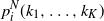 $p_i^N(k_1,\ldots,k_{K})$
that the offspring will be of type i. Note that we may have
 $p_i^N>0$
even if
 $k_i=0$
when we take mutations into account. Moreover, knowing that there are
 $k_1+ \cdots +k_{K}=k$
potential parents, such a configuration has probability
 \begin{equation*} \binom{k }{ k_1,\ldots,k_{K}}x_1^{k_1} \cdots x_{K}^{k_{K}}\end{equation*}
of being picked. Hence
 \begin{equation*} \mu_i(x)= \lim_{N \to \infty} \frac{1}{\rho_N} \biggl( \sum_{k=2}^{\infty} \pi_k^N \biggl( \sum_{k_1+ \cdots +k_{K}=k} \binom{k }{ k_1,\ldots,k_{K}} x_1^{k_1} \cdots x_{K}^{k_{K}}p_i^N(k_1,\ldots,k_{K})-x_i\biggr)\biggr). \end{equation*}
But note that for any K-tuple
 $(k_1,\ldots,k_K)$
of integers, and
 $(z,x) \in \Delta_K^2$
,
 \begin{align*} | x_1^{k_1} \cdots x_{K}^{k_{K}}-z_1^{k_1} \cdots z_{K}^{k_{K}} |& \leq | x_1^{k_1}-z_1^{k_1}| | x_2^{k_2} \cdots x_{K}^{k_{K}} |+z_1^{k_1} | x_2^{k_2} \cdots x_{K}^{k_{K}}-z_2^{k_2} \cdots z_{K}^{k_{K}} |\\* &\leq |x_1-z_1|+ | x_2^{k_2} \cdots x_{K}^{k_{K}}-z_2^{k_2} \cdots z_{K}^{k_{K}} |\\* &\leq \cdots \leq \sum_{j=1}^{K}|x_j-z_j|.\end{align*}
Hence
 \begin{align*} & | \mu_i(x)-\mu_i(z) | \\* &\quad \leq \lim_{N \to \infty} \frac{1}{\rho_N} \biggl[ \sum_{k=2}^{\infty} \pi_k^N \biggl( |x_i-z_i|\\* &\quad\quad\, + \sum_{k_1+ \cdots +k_{K}=k} \binom{k }{ k_1,\ldots,k_{K}}p_i^N(k_1,\ldots,k_{K}) | x_1^{k_1} \cdots x_{K}^{k_{K}}- z_1^{k_1} \cdots z_{K}^{k_{K}} |\biggr)\biggr]\\ & \quad = |x_i-z_i| \\* &\quad\quad\, +\lim_{N \to \infty} \frac{1}{\rho_N}\biggl[\!\sum_{k=2}^{\infty} \pi_k^N \biggl(\!\sum_{k_1+ \cdots +k_{K}=k} \binom{k }{ k_1,\ldots,k_{K}}p_i^N(\!k_1,\ldots,k_{K}) | x_1^{k_1} \cdots x_{K}^{k_{K}}- z_1^{k_1} \cdots z_{K}^{k_{K}} |\biggr)\!\biggr]\\* & \quad \leq C_i \sum_{j=1}^{K}|x_j-z_j|,\end{align*}
where
 $C_i$
is a finite constant. As a consequence,
 \begin{align*}| \langle \mu(x)-\mu(z),x-z\rangle | &\leq \sup_{1 \leq i \leq K}C_i \sum_{i,j=1}^{K} |x_i-z_i|\, |x_j-z_j|\\*&\leq \sup_{1 \leq i \leq K}C_i \sum_{i,j=1}^{K} (|x_i-z_i|^2+|x_j-z_j|^2 )\\*&\leq \sup_{1 \leq i \leq K}2C_i K |x-z|^2.\end{align*}
Now take
 $\zeta \equiv 1 $
in Assumption 2.1 and
 $\rho=C$
in Assumption 2.3 of [Reference Xi and Zhu51]. We have to check that the following inequalities hold for
 $(x,z) \in \Delta_K^2$
:
 \begin{align} \langle \mu(x),x\rangle + |\zeta(x)|^2 + \int_0^1 \int_0^1 |c(x,u,y)|^2 \,{\text{d}} u \frac{\Lambda({\text{d}} y)}{y^2} & \leq C (|x|^2+1) , \end{align}
 \begin{align} \langle \mu(x)-\mu(z),x-z\rangle + |\zeta(x)-\zeta(z)|^2 & \leq C |x-z|^2 , \end{align}
and
 \begin{equation} \int_0^1 \int_0^1 |c(x,u,y)-c(z,u,y)| \,{\text{d}} u \frac{\Lambda({\text{d}} y)}{y^2}\leq C |x-z| , \end{equation}
where
 $c_i(x,u,y)= y(\textbf{1}_{0 \leq u-(x_1+ \cdots +x_{i-1})<x_i}-x_i)$
and C is a positive constant, in order to apply Corollary 2.9 of [Reference Xi and Zhu51]. The function
 $\sigma$
and
 $\mu$
are bounded. Moreover,
 \begin{equation*} \int_0^1 \int_0^1 |c(x,u,y)|^2 \,{\text{d}} u \frac{\Lambda({\text{d}} y)}{y^2}\leq \int_0^1 \int_0^1 \,{\text{d}} u \Lambda({\text{d}} y)=\int_0^1 \Lambda({\text{d}} y), \end{equation*}
which is finite by assumption. Hence (5.1) holds. Let us now prove that (5.3) holds. We have
 \begin{align*}& \int_0^1 \int_0^1 |c_i(x,u,y)-c_i(z,u,y)| \,{\text{d}} u \frac{\Lambda({\text{d}} y)}{y^2} \\*&\quad = \int_0^1 \int_0^1 |(\textbf{1}_{0 \leq u-(x_1+ \cdots +x_{i-1})<x_i}-x_i)-(\textbf{1}_{0 \leq u-(z_1+ \cdots +z_{i-1})<z_i}-z_i)| \,{\text{d}} u \frac{\Lambda({\text{d}} y)}{y}\\* &\quad \leq ( 2|x_i-z_i|+|x_{i-1}-z_{i-1}| ) \int_0^1 \frac{\Lambda({\text{d}} y)}{y},\end{align*}
with the convention
 $x_{-1}=z_{-1}=0$
. Hence (5.3) holds with
 $C = 3\int_{(0,1]}\Lambda({\text{d}} y)/y$
. This proves that (3.5) admits a unique strong solution under assumption (2).
To obtain a general result in multiple dimensions we would need to verify that assumption (5.2) holds. Let us focus on
 $\zeta$
and see what the problem is. For
 $i \in E$
we have
 \begin{align*} |\zeta_{ii}(x) - \zeta_{ii}(z) |^2 & =\biggl|\sqrt{ \frac{x_i(1-x_1 \cdots -x_i)}{1-x_1 \cdots -x_{i-1}} } -\sqrt{ \frac{z_i(1-z_1 \cdots -z_i)}{1-z_1 \cdots -z_{i-1}} } \biggr|^2\\*& \leq \biggl| \frac{x_i(1-x_1 \cdots -x_i)}{1-x_1 \cdots -x_{i-1}}-\frac{z_i(1-z_1 \cdots -z_i)}{1-z_1 \cdots -z_{i-1}} \biggr| \\*& <|x-z|,\end{align*}
where we have used the fact that for
 $a,b \geq 0$
,
 $|a-b|^2 \leq |a-b||a+b|= |a^2-b^2|$
. For
 $j > i \in E^2$
,
 \begin{equation*} |\zeta_{ij}(x) - \zeta_{ij}(z) |^2 =0, \end{equation*}
and for
 $j < i \in E^2$
,
 \begin{align*} & |\zeta_{ij}(x) - \zeta_{ij}(z) |^2 \\* &\quad =\biggl|x_i \sqrt{ \frac{x_j}{(1-x_1 \cdots -x_{j-1})(1-x_1 \cdots -x_j)} } -z_i \sqrt{ \frac{z_j}{(1-z_1 \cdots -z_{j-1})(1-z_1 \cdots -z_j)} } \biggr|^2\\&\quad \leq \biggl| \frac{x_i^2 x_j}{(1-x_1 \cdots -x_{j-1})(1-x_1 \cdots -x_j)} -\frac{z_i^2z_j}{(1-z_1 \cdots -z_{j-1})(1-z_1 \cdots -z_j)} \biggr|\\*& \quad <3|x-z|.\end{align*}
Unfortunately, it is not enough to apply Corollary 2.9 of [Reference Xi and Zhu51]; we would need
 $|x-y|^2$
.
However, it is exactly what one needs to apply Theorem 5.1 of [Reference Li and Pu42], which works only in the case
 $K=2.$
To be more precise, to check that the result is true under condition (1), we need to check conditions (2.a), (2.b), (5.a), (5.b), and (5.c) of [Reference Li and Pu42]. The calculations are either already done in the previous lines, or very similar, so we do not give the details. Note that similarly to the case of [Reference González Casanova and Spanò29], the assumption
 $\int_0^\infty \Lambda({\text{d}} y)/y$
is not needed in this case. The finiteness of
 $\Lambda([0,1])$
is enough. We conclude that the result also follows under hypothesis (1).
To prove statement (3) we will make a change of variable and apply Lemma 3.6 of [Reference González Casanova and Spanò29]. Let us choose
 $i_0 \in [K-1] $
and consider the process
 \begin{equation*} (Y_{i_0}(t), t \geq 0)\,:\!= ((X_1+ \cdots +X_{i_0})(t), t\geq 0) .\end{equation*}
Adding the
 $i_0$
equations, and recalling that (4.2) implies that for
 $x \in \Delta_K$
 \begin{equation*} \sum_{i=1}^{i_0} \mu_i(x)= \sum_{k=1}^\infty \pi_k ( (x_1+ \cdots +x_{i_0})^{k+1}-(x_1+ \cdots +x_{i_0})), \end{equation*}
 $Y_{i_0}$
should be the solution to
 \begin{align*} {\text{d}} Y_{i_0}(t) & = \kappa \sum_{k=1}^\infty \pi_k ( Y_{i_0}^{k+1}(t)-Y_{i_0}(t)) \,{\text{d}} t + \sqrt{\sigma} \sum_{i=1}^{i_0} \sum_{j=1}^{K}\zeta_{ij}(X(t)) \,{\text{d}} B^{(j)}_t \notag \\* &
\quad\, + \sum_{i=1}^{i_0} \int_0^1 \int_0^1 z \Bigl( \textbf{1}_{\big\{ \sum_{j=1}^{i-1}X_j(t-\!) \leq u < \sum_{j=1}^{i}X_j(t-\!) \big\}}-X_i(t-\!) \Bigr) \tilde{N}({\text{d}} t, {\text{d}} u, {\text{d}} z).\end{align*}
Note first that the jump term may be reduced to
 \begin{equation*} \int_0^1 \int_0^1 z \bigl( \textbf{1}_{\{ u
< Y_{i_0}(t-\!) \}}-Y_{i_0}(t-\!) \bigr) \tilde{N}({\text{d}} t, {\text{d}} u, {\text{d}} z). \end{equation*}
Let us now focus on the diffusion term. By definition of
 $Y_{i_0}$
, using the calculations derived in the proof of Proposition 3.2 we obtain
 \begin{align*} \frac{ {\text{d}} \langle Y_{i_0},Y_{i_0} \rangle}{{\text{d}} t} & = \frac{{\text{d}} \langle X_1+ \cdots + X_{i_0},X_1+ \cdots +X_{i_0} \rangle}{{\text{d}} t} \\* & = \sum_{i=1}^{i_0} \,{\text{d}} \langle X_i,X_i \rangle + \sum_{1 \leq i,j \leq i_0, i \neq j} {\text{d}} \langle X_i,X_j \rangle\displaybreak\\& = \sigma\sum_{i=1}^{i_0} X_i(1-X_i) - \sigma\sum_{1 \leq i,j \leq i_0, i \neq j} X_iX_j\\ & = \sigma\sum_{i=1}^{i_0} X_i\biggl(1-X_i - \sum_{1 \leq j \leq i_0, i \neq j} X_j \biggr)\\& = \sigma(X_1+ \cdots +X_{i_0})(1-X_1- \cdots -X_{i_0}) \\* & = \sigma Y_{i_0}(1-Y_{i_0}).\end{align*}
In particular, it implies that there exists a Brownian motion
 $W^{(i_0)}$
such that (see e.g. [Reference Durrett21, Theorem (4.4)])
 \begin{equation*}\sqrt{\sigma} \sum_{i=1}^{i_0} \sum_{j=1}^{K}\zeta_{ij}(X(t))\,{\text{d}} B^{(j)}_t = \sqrt{ \sigma Y_{i_0}(t)( 1 - Y_{i_0}(t) )}\,{\text{d}} W^{(i_0)}_t, \end{equation*}
and thus
 $Y_{i_0}$
should be the solution to
 \begin{align*} {\text{d}} Y_{i_0}(t) &= \kappa \sum_{k=1}^\infty \pi_k ( Y_{i_0}^{k+1}(t)-Y_{i_0}(t))\,{\text{d}} t +\sqrt{ \sigma Y_{i_0}(t)( 1 - Y_{i_0}(t) )}\,{\text{d}} W^{(i_0)}_t \notag \\* &\quad\, + \int_0^1 \int_0^1 z \bigl( \textbf{1}_{\{ u
< Y_{i_0}({t^-}) \}}-Y_{i_0}({t^-}) \bigr) \tilde{N}({\text{d}} t, {\text{d}} u, {\text{d}} z).\end{align*}
But from Lemma 3.6 of [Reference González Casanova and Spanò29] we know that this equation has a unique strong solution. We can use the same reasoning to prove that
 $Y_{i_0-1}$
(if
 $i_0>1$
) is the unique strong solution to
 \begin{align*} {\text{d}} Y_{i_0-1}(t)& = \kappa \sum_{k=1}^\infty \pi_k ( Y_{i_0-1}^{k+1}(t)-Y_{i_0-1}(t))\,{\text{d}} t +\sqrt{ \sigma Y_{i_0-1}(t)( 1 - Y_{i_0-1}(t) )}\,{\text{d}} W^{(i_0-1)}_t \notag \\* &\quad\, + \int_0^1 \int_0^1 z \bigl( \textbf{1}_{\{ u
< Y_{i_0-1}(t-\!) \}}-Y_{i_0-1}(t-\!) \bigr) \tilde{N}({\text{d}} t, {\text{d}} u, {\text{d}} z),\end{align*}
where
 $W^{(i_0-1)}$
is uniquely determined from the Brownian motions
 $(B^{(j)}, 1 \leq j \leq K)$
. As
 $X_{i_0}= Y_{i_0}-Y_{i_0-1}$
, this concludes the proof.
Proof of Lemma 3.1. Assume that the hypotheses of Lemma 3.1 hold. In the proof of Corollary 3.1 we saw that the reason why we could not ensure the existence of a strong solution was that all the
 $\zeta_{ij}$
had not bounded continuous partial derivatives on
 $\Delta_K$
. But for any
 $0 < \varepsilon < 1/2$
, there exists a finite constant
 $C(\varepsilon)$
such that, for x in
 $(\varepsilon,1-\varepsilon)^K$
and
 $(i,j,k) \in E^2$
,
 \begin{equation*} \biggl|\frac{\partial \zeta_{ij}(x)}{\partial_k}\biggr| \leq C(\varepsilon). \end{equation*}
As a consequence, applying the Taylor formula we get, for x, z in
 $(\varepsilon,1-\varepsilon)^K$
,
 \begin{equation*} |\zeta_{ij}(x) - \zeta_{ij}(z) |^2 \leq K C(\varepsilon) |x-z|^2. \end{equation*}
We can thus apply Corollary 2.9 of [Reference Xi and Zhu51] and conclude.
5.2. Proofs of general results on the selective functions
Proof of Lemma 3.2. For each
 $N\in{\mathbb{N}}^*$
consider the random graph with parameters
 \begin{equation*}Q_N=(1-\rho_N)\delta_1+\rho_N\delta_N\end{equation*}
and colouring rule
 $c^N_{z}=g(z/N)$
for every N-dimensional vector z and
 $c^N_{z}=\delta_{z}$
for every one-dimensional vector z. Note that this is indeed a colouring rule because we assumed that
 $g\colon \Delta_K\mapsto \Delta_K.$
For every
 $i\in E$
, note that
 \begin{equation*}p^N_i(x)=\sum_{z \in E^N} {\mathbb{P}}_{x}(z_v=z)c^N_{z}(i).\end{equation*}
Observe that
 $z_v$
is a multinomial random variable with parameters x and 1 with probability
 $1-\rho_N$
, and is a multinomial random variable with parameters x and N with probability
 $\rho_N$
. Hence
 \begin{equation*}p_i^N(x)={\mathbb{E}}[c^N_{z_v}]=(1-\rho_N)x_i+\rho_N{\mathbb{E}}\biggl[g_i\biggl(\frac{z_v}{N}\biggr)\biggr] = x_i + \rho_N (g_i(x)-x_i)+ {\text{o}}(\rho_N), \quad {N \to \infty,}\end{equation*}
where in the right-hand side we used the law of large numbers. The rest of the proof consists in applying Theorem 3.1.
Proof of Lemma 3.3. The proof is similar to the proof of Lemma 3.2 and follows the observation that by construction
 \begin{equation*}\mu_i(x)=g_i(x)-x_i\end{equation*}
for all
 $i \in E$
and
 $x \in \Delta_K$
.
5.3. Proofs of general results on allele extinction and fixation
Proof of Proposition 3.3. Recall the definition of the ancestral process
 $(D_t, t \geq 0)$
in (4.3). Then, if one of the conditions of Proposition 3.3 is satisfied, the process
 $(D_t, t \geq 0)$
is positive recurrent (see [Reference Griffiths30, Theorem 3] and [Reference Foucart26, Theorem 1.1]). In particular, it will reach one in finite time almost surely. This means that all the individuals in the population at a given time will have the same ancestor. As we did not allow for mutations in this proposition, it implies that all the descendants of this ancestor (i.e. all the individuals alive at subsequent generations and related to this ancestor by a sequence of edges) will have the same type.
The proof of Proposition 3.4 is based on the following two lemmas.
Lemma 5.1. Assume that the process
 $Z=(Z_t, t \geq 0)$
satisfies an equation of the form
 \begin{equation*} {\text{d}} Z_t = (1-Z_t)S(Z_t,t)\,{\text{d}} t + \sqrt{Z_t(1-Z_t)}\,{\text{d}} B_t, \quad Z_0 \in (0,1){,}\end{equation*}
where B is a Brownian motion, and for all
 $t \geq 0$
and
 $z \in [0,1]$
,
 $|S(z,t)|\leq C <\infty$
and
 $S(0,t)=0$
. Then
 $Z_t \in [0,1]$
for all
 $t \geq 0$
, and
 \begin{equation*} \int_0^{T_1} \frac{1}{1-Z_s}\,{\text{d}} s = \infty \quad {a.s.}, \end{equation*}
where for
 $a \in [0,1]$
,
 $ T_a\,:\!= \inf \{ t \geq 0, Z_t=a \}. $
Lemma 5.2. Let
 $n \geq 3 $
be in
 ${\mathbb{N}}^*$
and
 $V=(V_1(t),\ldots,V_{n-1}(t), t \geq 0)$
be a process with (possibly inhomogeneous) infinitesimal generator acting on f at
 $v \in \Delta_{n-1} $
of the form
 \begin{equation*} \mathcal{A}_tf(v)= \sum_{i=1}^{n-1} \mu_i(v,t) \frac{\partial f}{\partial v_i}(v)+\sigma \sum_{i,j=1}^{n-1} \sigma_{ij}(v) \frac{\partial^2 f}{\partial v_i v_j}(v), \end{equation*}
where
 $\mu$
is continuous with respect to v and can be written as
 \begin{equation*}\mu(v,t)=(v_i(1-v_i)s_i(v,t),1 \leq i \leq n),\end{equation*}
with
 $\|s\|_\infty\leq C$
for a finite C, and
 \begin{equation*}\sigma(v)=((1_{\{j=i\}}-v_j)v_i,1 \leq i,j \leq n).\end{equation*}
For all
 $t \geq 0$
, let
 \begin{equation*}1-V_n(t)= V_1(t)+ \cdots +V_{n-1}(t),\end{equation*}
and define the time change
 $\tau$
on
 $[0,\infty)$
by
 \begin{equation*} \int_0^{\tau(t)}\frac{1}{1-V_n(s)}\,{\text{d}} s=t \quad \text{{for all} } t \geq 0. \end{equation*}
Next let us introduce the process
 \begin{align*} Y & =(Y_1(t),\ldots,Y_{n-2}(t), 1- Y_1(t)- \cdots -Y_{n-1}(t),t \geq 0) \\* & \,:\!= \biggl( \frac{V_1}{1-V_n}(\tau(t)),\ldots, \frac{V_{n-2}}{1-V_n} (\tau(t)), \frac{V_{n-1}}{1-V_n}(\tau(t)) ,t \geq 0\biggr) .\end{align*}
Then the stochastic process Y has a (possibly inhomogeneous) infinitesimal generator acting on f at
 $y \in \Delta_{n-1} $
of the form
 \begin{equation*} \mathcal{\tilde{A}}_tf(y)= \sum_{i=1}^n \tilde{\mu}_i(y,t) \frac{\partial f}{\partial y_i}(y) +\sigma \sum_{i,j=1}^n \sigma_{ij}(y) \frac{\partial^2 f}{\partial y_i y_j}(y), \end{equation*}
where
 $\tilde{\mu}$
is continuous with respect to v and can be written as
 \begin{equation*}\tilde{\mu}(y,t)=(y_i(1-y_i)\tilde{s}_i(y,t),1 \leq i \leq n-1),\end{equation*}
with
 $\|\tilde{s}\|_\infty\leq C'$
for a finite
 $C'$
, and
 \begin{equation*}\sigma(y)=((1_{\{j=i\}}-y_j)y_i,1 \leq i,j \leq n-1).\end{equation*}
Before proving these two lemmas, we prove Proposition 3.4.
Proof of Proposition 3.4. The fact that one of the alleles ultimately fixates is a consequence of Proposition 3.3. If
 $n=2$
, the result is immediate. Hence we assume that
 $n \geq 3$
. From Lemma 5.1,
 \begin{equation*} \int_0^{T_1^{V_n}}\frac{1}{1-V_n(s)}\,{\text{d}} s=\infty, \end{equation*}
where
 $T_1^{V_n}$
is the hitting time of 1 by the process
 $V_n$
. Indeed,
 \begin{equation*} \biggl| - \sum_{i=1}^{n-1} \mu_i(V(t),t) \biggr| \leq \sum_{i=1}^{n-1} V_i(t)(1-V_i(t)) |s_i(V(t),t)|\leq C \sum_{i=1}^{n-1} V_i(t) = C ( 1-V_n(t) ).\end{equation*}
We may thus introduce the time change
 $\tau$
on
 $[0,\infty)$
such that
 \begin{equation*} \int_0^{\tau(t)}\frac{1}{1-V_n(s)}\,{\text{d}} s=t \quad \text{{for all} } t \geq 0. \end{equation*}
As for any
 $t <\infty $
,
 $V_n(\tau(t))<1$
, we may consider the process
 \begin{equation*} Y(t)=(Y_1(t),\ldots,Y_{n-2}(t))\,:\!= \biggl( \frac{V_1(\tau(t))}{1-V_n(\tau(t))},\ldots,\frac{V_{n-2}(\tau(t))}{1-V_n(\tau(t))} \biggr). \end{equation*}
Thanks to Lemma 5.2, we know that the stochastic process
 $(Y_1(t),\ldots,Y_{n-2}(t))_{t \geq 0}$
has a (possibly inhomogeneous) infinitesimal generator acting on f at
 $y \in \Delta_{n-2} $
of the form
 \begin{equation*} \mathcal{\tilde{A}}_tf(y)= \sum_{i=1}^{n-2} \tilde{\mu}_i(y,t) \frac{\partial f}{\partial y_i}(y) +\sigma \sum_{i,j=1}^{n-2} \sigma_{ij}(y) \frac{\partial^2 f}{\partial y_i y_j}(y), \end{equation*}
where
 \begin{equation*}\tilde{\mu}(y,t)=(y_i(1-y_i)\tilde{s}_i(y,t),1 \leq i \leq n-2),\end{equation*}
 $|\tilde{s}|\leq C'$
for a finite
 $C'$
, and
 \begin{equation*}\sigma(y)=((1_{\{j=i\}}-y_j)y_i,1 \leq i,j \leq n-2).\end{equation*}
We end the proof following the proof of Theorem 2.1 of [Reference Coron, Méléard and Villemonais19]. By the induction hypothesis, the process Y undergoes
 $n-2$
successive extinctions at times
 \begin{equation*} E_1^{Y}< \cdots <E_{n-2}^{Y}<\infty. \end{equation*}
Hence
 \begin{equation*} \tau(E_1^{Y})< \cdots <\tau(E_{n-2}^{Y})<\tau(\infty)=T_1^{V_n}. \end{equation*}
If
 $\{ T_1^{V_n}< \infty \}$
, the times
 $ \tau(E_1^{Y}), \ldots, \tau(E_{n-2}^{Y})$
,
 $T_1^{V_n}$
correspond to the
 $n-1$
extinction times of alleles
 $\{1,2,\ldots,n-1\}$
. This concludes the proof, as from the first part of the theorem we know that
 \begin{align*} {\mathbb{P}}\biggl(\bigcup_{i=1}^n \{T_1^{V_i}<\infty\}\biggr)=1. \\[-42pt] \end{align*}
To prove Lemma 5.1, we cannot use general results of [Reference Coron, Méléard and Villemonais19] because of the selection term. We will instead apply Itô’s formula to an auxiliary function of the process Z.
Proof of Lemma 5.1. First note that Z is continuous and that the states 0 and 1 are absorbing. This implies that Z stays in the interval [0, 1]. Let
 $\varepsilon,Z_0>0$
be such that
 $Z_0<1-\varepsilon$
. By applying Itô’s formula to the function
 $f(x)\,:\!=- \ln (1-x)$
, we get for any positive t
 \begin{align*}& - \ln ( 1- Z_{t \wedge T_{1-\varepsilon}} )+ \ln (1-Z_0) \\* & \quad =\int_0^{t \wedge T_{1-\varepsilon}} S(Z_s,s)\,{\text{d}} s + \int_0^{t \wedge T_{1-\varepsilon}} \sqrt{\frac{Z_s}{1-Z_s}}\,{\text{d}} B_s + \frac{1}{2} \int_0^{t \wedge T_{1-\varepsilon}}\frac{Z_s}{1-Z_s}\,{\text{d}} s.\end{align*}
We have
 \begin{equation*} {\mathbb{P}}\Bigl( \lim_{\varepsilon \to 0^+} \{- \ln ( 1- Z_{T_{1-\varepsilon}} )+ \ln (1-Z_0)\}= \infty, T_1 < \infty \Bigr)={\mathbb{P}}(T_1
< \infty), \end{equation*}
and
 \begin{equation*} {\mathbb{P}}\biggl( \limsup_{\varepsilon \to 0^+}\, \biggl|\int_0^{T_{1-\varepsilon}} S(Z_s,s)\,{\text{d}} s\biggr|< \infty,T_1 < \infty \biggr)= {\mathbb{P}}(T_1
< \infty), \end{equation*}
as S is bounded by assumption. We deduce
 \begin{equation} {\mathbb{P}}\biggl( \lim_{\varepsilon \to 0^+} \biggl\{\int_0^{T_{1-\varepsilon}} \sqrt{\frac{Z_s}{1-Z_s}}\,{\text{d}} B_s + \int_0^{T_{1-\varepsilon}}\frac{Z_s}{1-Z_s}\,{\text{d}} s\biggr\}= \infty, T_1 < \infty \biggr)= {\mathbb{P}}(T_1
< \infty).\end{equation}
We will now prove that (5.4) implies the following property:
 \begin{equation} {\mathbb{P}}\biggl(\int_0^{T_{1}}\frac{Z_s}{1-Z_s}\,{\text{d}} s= \infty, T_1 < \infty \biggr)= {\mathbb{P}}(T_1
< \infty).\end{equation}
The random variable
 \begin{equation*} \int_0^{T_{1-\varepsilon}}\frac{Z_s}{1-Z_s}\,{\text{d}} s \end{equation*}
is non-negative and non-increasing with
 $\varepsilon$
. As a consequence it has a non-negative limit when
 $\varepsilon$
goes to 0, which can be finite or infinite. Let us consider a measurable event A such that
 \begin{equation} \lim_{\varepsilon \to 0^+} \biggl\{\int_0^{T_{1-\varepsilon}}\frac{Z_s}{1-Z_s}\,{\text{d}} s\biggr\}=\int_0^{T_1}\frac{Z_s}{1-Z_s}\,{\text{d}} s< \infty \quad \text{a.s. on } A \cap \{T_1
< \infty\}.\end{equation}
Then from (5.4) we get that
 \begin{equation} \lim_{\varepsilon \to 0^+} \biggl\{\int_0^{T_{1-\varepsilon}}\sqrt{\frac{Z_s}{1-Z_s}}\,{\text{d}} B_s\biggr\}= \infty \quad \text{a.s. on } A \cap \{T_1
< \infty\}.\end{equation}
Let us introduce the process
 \begin{equation*} M^{(\varepsilon)}_t\,:\!=\int_0^{t \wedge T_{1-\varepsilon}} \sqrt{\frac{Z_s}{1-Z_s}}\,{\text{d}} B_s. \end{equation*}
 $ M^{(\varepsilon)}$
is a continuous martingale. In particular, it is a time change of a Brownian motion, and there exists a Brownian motion W such that (see e.g. [Reference Durrett21, Theorem (4.4)])
 \begin{equation*} M^{(\varepsilon)}_t = W_{\int_0^{t \wedge T_{1-\varepsilon}}{{Z_s}/{(1-Z_s)}}\,{\text{d}} s}. \end{equation*}
This implies
 \begin{align*} & {\mathbb{E}} \biggl[ \textbf{1}_{A \cap \{T_1 < \infty\}} \,{\exp {\biggl(- \int_0^{t \wedge T_{1-\varepsilon}} \sqrt{\frac{Z_s}{1-Z_s}}\,{\text{d}} B_s}\biggr)} \biggr] \\* &\quad = {\mathbb{E}} \biggl[ \textbf{1}_{A \cap \{T_1 < \infty\}} \,{\exp{\biggl(- W_{\int_0^{t \wedge T_{1-\varepsilon}}{{Z_s}/{(1-Z_s)}}\,{\text{d}} s}\biggr)}} \biggr]\\* & \quad\geq {\mathbb{E}} \biggl[ \textbf{1}_{A \cap \{T_1
< \infty\}} \,{\exp{\biggl(- \sup \biggl\{ W_u,u \leq \int_0^{t \wedge T_{1-\varepsilon}}\frac{Z_s}{1-Z_s}\,{\text{d}} s\biggr\}\biggr)}} \biggr].\end{align*}
As
 $\{T_1 < \infty\}$
implies
 $\{T_{1-\varepsilon} < \infty\}$
, we may let t go to infinity, and obtain
 \begin{align} & \notag {\mathbb{E}} \biggl[ \textbf{1}_{A \cap \{T_1 < \infty\}} \,{\exp{\biggl(- \int_0^{T_{1-\varepsilon}} \sqrt{\frac{Z_s}{1-Z_s}}\,{\text{d}} B_s\biggr)}} \biggr]\\* & \quad \geq {\mathbb{E}} \biggl[ \textbf{1}_{A \cap \{T_1 < \infty\}} \,{\exp{\biggl(- \sup \biggl\{ W_u,u \leq \int_0^{T_{1-\varepsilon}}\frac{Z_s}{1-Z_s}\,{\text{d}} s\biggr\}\biggr)}} \biggr] \notag \\* & \quad \geq {\mathbb{E}} \biggl[ \textbf{1}_{A \cap \{T_1
< \infty\}} \,{\exp {\biggl(- \sup \biggl\{ W_u,u \leq \int_0^{T_1}\frac{Z_s}{1-Z_s}\,{\text{d}} s\biggr\}\biggr)}} \biggr].\end{align}
But from (5.7), we get that
 \begin{equation*} \lim_{\varepsilon \to 0}{\mathbb{E}} \biggl[ \textbf{1}_{A \cap \{T_1
< \infty\}} \,{\exp{\biggl(- \int_0^{T_{1-\varepsilon}} \sqrt{\frac{Z_s}{1-Z_s}}\,{\text{d}} B_s\biggr)}} \biggr]=0, \end{equation*}
and (5.6) implies that the right-hand side of (5.8) is positive if and only if the event
 $A \cap \{T_1 < \infty\}$
has a positive probability. We thus deduce that
 \begin{equation*} {\mathbb{P}} ( A \cap \{T_1
< \infty\})=0, \end{equation*}
which implies (5.5). We conclude the proof of Lemma 5.1 by noting that
 \begin{align*} {\mathbb{P}}\biggl( \int_0^{T_{1}}\frac{1}{1-Z_s}\,{\text{d}} s = \infty, T_1 = \infty \biggr)= {\mathbb{P}}(T_1 = \infty).\\[-40pt] \end{align*}
Proof of Lemma 5.2. Let
 $\tilde{\mathcal{L}}$
denote the infinitesimal generator of the process
 \begin{equation*} \biggl( \frac{V_1}{1-V_n}(t),\ldots, \frac{V_{n-2}}{1-V_n}(t), 1-V_n(t) \biggr)_{t \geq 0}. \end{equation*}
For any real-valued function f defined on
 $\{ (y_1,\ldots,y_{n-2},1-x_n) \in\Delta_{n-2}\times \Delta_1 \}$
, twice differentiable, we can write for
 $x_n \neq 1$
,
 \begin{equation*} \tilde{\mathcal{L}}f (y_1,\ldots,y_{n-2},1-x_n) \eqqcolon \mathcal{L}({\kern1.3pt}f \circ g)(x_1,\ldots,x_{n-1}), \end{equation*}
where by definition, for
 $(x_1,\ldots,x_{n-1}) \in [0,1]^{n-1}$
such that
 $0<x_1+ \cdots +x_{n-1}\leq 1$
,
 \begin{align*} y & =(y_1,\ldots,y_{n-2},1-x_n) \\* & = g(x_1,\ldots,x_{n-1})\\* & = \biggl( \frac{x_1}{x_1+ \cdots +x_{n-1}}, \ldots, \frac{x_{n-2}}{x_1+ \cdots +x_{n-1}},\, x_1+ \cdots +x_{n-1} \biggr). \end{align*}
It can be verified that
 \begin{align*} \mathcal{L}f(x)= \mathcal{L}f(x_1, \cdots x_{n-1})\,:\!= \sum_{i=1}^{n-1}\mu_i(x)\frac{\partial f}{\partial x_i}(x) + \sum_{i=1}^{n-1}x_i(1-x_i)\frac{\partial^2 f}{\partial x_i^2}(x) - \sum_{i\neq j=1}^{n-1}x_ix_j\frac{\partial^2 f}{\partial x_i x_j}(x).\end{align*}
The calculations for the diffusion part of
 $\tilde{\mathcal{L}}$
have been done in [Reference Coron, Méléard and Villemonais19]. We thus only need to compute the term of drift. Hence
 \begin{align*} A(x) & \,:\!= \sum_{i=1}^{n-1} \mu_i(x) \frac{ \partial }{\partial x_i}({\kern1.3pt}f\circ g (x))\\*& = \sum_{i=1}^{n-2} \mu_i(x) \biggl(\sum_{j=1}^{n-2} \frac{ \partial y_j }{\partial x_i} \frac{\partial f}{\partial y_j}( y)+ \frac{ \partial (1-x_n) }{\partial x_i} \frac{\partial f}{\partial (1-x_n)} ( y)\biggr)\\*& \quad\, + \mu_{n-1}(x)\biggl(\sum_{j=1}^{n-2} \frac{ \partial y_j }{\partial (1-x_n)} \frac{\partial f}{\partial y_j}( y) + \frac{\partial f}{\partial (1-x_n)} ( y)\biggr)\\& = \sum_{i=1}^{n-2} \mu_i(x) \biggl(\sum_{j=1, j \neq i}^{n-2} \frac{- x_j }{(1-x_n)^2} \frac{\partial f}{\partial y_j}(y) + \frac{(1-x_n)-x_i}{(1-x_n)^2} \frac{\partial f}{\partial y_i} (y) + \frac{\partial f}{\partial (1-x_n)}( y)\biggr)\\*& \quad\, + \mu_{n-1}(x)\biggl(\sum_{j=1}^{n-2} \frac{ -x_j }{(1-x_n)^2} \frac{\partial f}{\partial y_j}(y) + \frac{\partial f}{\partial (1-x_n)} (y)\biggr).\end{align*}
Rearranging the terms, we get
 \begin{equation*} A(x) = \frac{1}{1-x_n}\biggl( \sum_{i=1}^{n-2} \biggl( \mu_i(x) - y_i \sum_{j=1}^{n-1}\mu_j(x) \biggr) \frac{\partial f}{\partial y_i}(y)\biggr)+ \sum_{j=1}^{n-1}\mu_j(x) \frac{\partial f}{\partial (1-x_n)} ( y). \end{equation*}
If we introduce the notation
 \begin{equation*} \tilde{\mu}_i(y,x)= \mu_i(x) - y_i \sum_{j=1}^{n-1}\mu_j(x), \end{equation*}
we get, adding the diffusive part,
 \begin{align*} \tilde{\mathcal{L}}(y)& = \frac{1}{1-x_n} \sum_{i=1}^{n-2} \biggl( \tilde{\mu}_i(y,x) \frac{\partial f}{\partial y_i}(y)+ \sigma y_i (1- y_i)\frac{\partial^2 f}{\partial y_i^2}(y)- \sum_{j = 1, j \neq i}^{n-2}y_i y_j\frac{\partial^2 f}{\partial y_i \partial y_j}(y)\biggr)\\*&\quad\, + \sum_{i=1}^{n-1}\mu_i(x) \frac{\partial f}{\partial (1-x_n)} ( y) + \sigma x_n(1-x_n) \frac{\partial^2 f}{\partial (1-x_n)^2}(y).\end{align*}
This proves that the diffusive part of the process Y is the same as the diffusive part of an
 $(n-2)$
-dimensional Wright–Fisher process. We still have to prove that
 $\tilde{\mu}$
satisfies the assumptions we want.
 $\tilde{\mu}$
can be rewritten in two different ways. Firstly we have
 \begin{align} \tilde{\mu}_i(y,x)& = x_i(1-x_i) s_i(x) - y_i \sum_{j=1}^{n-1}\mu_j(x) = y_i \biggl( (1-x_n)(1-x_i)s_i(x)- \sum_{j=1}^{n-1}\mu_j(x) \biggr). \end{align}
Secondly
 \begin{align} \tilde{\mu}_i(y,x)& = (1-y_i) \mu_i(x) - y_i \sum_{j=1, j \neq i}^{n-1}\mu_j(x) = (1-y_i) \mu_i(x) - y_i \sum_{j=1, j \neq i}^{n-1}x_j(1-x_j)s_j(x).\end{align}
Let us focus on the last term. By the assumption, we know that there exists a finite C such that for any
 $x \in \Delta_{n-1}$
, and for
 $1 \leq j \leq n-1$
,
 \begin{equation*} | y_i (1-x_j)s_j(x) | \leq C .\end{equation*}
Hence we get
 \begin{align} \biggl|y_i \sum_{j=1, j \neq i}^{n-1}x_j(1-x_j)s_j(x) \biggr| & \leq C \sum_{j=1, j \neq i}^{n-1}x_j = C(1- x_i-x_n) = C(1-x_n)(1-y_i).\end{align}
Thus, from (5.9), we deduce that there exists a finite
 $C'$
such that
 \begin{equation*} \limsup_{y \in [0,1]^{n-1}, x \in \Delta_{n-1}, y_i \to 0^+} \frac{|\tilde{\mu}_i(y,x)|}{y_i(1-y_i)}<C', \end{equation*}
and from (5.10) and (5.11) we deduce that
 \begin{equation*} \limsup_{y \in [0,1]^{n-1}, x \in \Delta_{n-1},y_i \to 1^-} \frac{|\tilde{\mu}_i(y,x)|}{y_i(1-y_i)}<C'. \end{equation*}
As we are working on compact sets, we obtain that for
 $1 \leq i \leq n-2$
,
 $\tilde{\mu}_i(y,x)/(y_i(1-y_i))$
is continuous with respect to y. This concludes the proof.
5.4. Proofs of results on specific examples
Proof of Lemma 3.4. From Remark 3.3, we know that it is enough to check that in the examples under consideration,
 $\mu_i(x)/(1-x_i)$
is bounded, for
 $i \in E$
and
 $x \in \Delta_K$
.
Transitive ordering case. Recall that according to (4.2),
 \begin{equation*} \mu_i(x) = \sum_{j=1}^\infty \pi_j ((x_0+ \cdots +x_i)^{j+1}-(x_0+ \cdots +x_{i-1})^{j+1}-x_i).\end{equation*}
We can rewrite
 $\mu_i$
as the sum of two functions
 $\alpha_i$
and
 $\beta_i$
as follows:
 \begin{align*}\mu_i(x) & = \sum_{j=1}^\infty \pi_j\biggl(x_i\sum_{k=0}^j (x_0+ \cdots +x_i)^{k}(x_0+ \cdots +x_{i-1})^{j-k} -x_i\biggr) \\*& = x_i\sum_{j=1}^\infty \pi_j\biggl(\sum_{k=0}^j (x_0+ \cdots +x_i)^{k}(x_0+ \cdots +x_{i-1})^{j-k} -1\biggr) \\& = \underbrace{ x_i \sum_{j=1}^\infty \pi_j((x_0+ \cdots +x_i)^{j}-1)}_{\alpha_i}\\*&\quad\, +\underbrace{x_i (x_0+ \cdots +x_{i-1})\sum_{j=1}^\infty \pi_j\sum_{k=0}^{j-1} (x_0+ \cdots +x_i)^{k}(x_0+ \cdots +x_{i-1})^{j-k-1}}_{\beta_i}.\end{align*}
First note that
 \begin{align*} |\alpha_i|&= x_i \sum_{j=1}^\infty \pi_j (1-(x_0+ \cdots +x_i)^{j})\\* & = x_i (1-(x_0+ \cdots +x_i)) \sum_{j=1}^\infty \pi_j \biggl(\sum_{k=0}^{j-1}(x_0+ \cdots +x_i)^{k}\biggr)\\ & \leq x_i (1-x_i) \sum_{j=1}^\infty j \pi_j \\* & = x_i (1-x_i) \beta,\end{align*}
where we recall that
 $\beta$
was defined in (v) of Proposition 3.1. Second, we have
 \begin{align*} |\beta_i|&= x_i (x_0+ \cdots +x_{i-1})\sum_{j=1}^\infty \pi_j\biggl(\sum_{k=0}^{j-1} (x_0+ \cdots +x_i)^{k}(x_0+ \cdots +x_{i-1})^{j-k-1}\biggr)\\*&\leq x_i (1-x_i)\sum_{j=1}^\infty j\pi_j \\*& = x_i (1-x_i) \beta. \end{align*}
As a consequence,
 \begin{equation*} |\mu_i(x)|\leq 2 \kappa \beta x_i(1-x_i). \end{equation*}
RPS or food web case. For
 $ i \in E$
,
 \begin{equation*} |\mu_i(x)|= x_i\biggl| \sum_{ j \neq i, j<i}x_j-\sum_{ j \neq i, i<j}x_j \biggr| \leq x_i\biggl( \sum_{ j \neq i, j<i}x_j+\sum_{ j \neq i, i<j}x_j \biggr) \leq 2 x_i (1-x_i). \end{equation*}
Negative frequency-dependent selection. Recall that when the distribution of
 $K_v$
is concentrated on
 $\{1,3\}$
, we get
 \begin{equation*} \mu_i(x)=2 x_i\biggl[ \sum_{j \neq i} x_j^2-x_i(1-x_i) \biggr]. \end{equation*}
As
 \begin{equation*} \sum_{j \neq i} x_j^2\leq \sum_{j \neq i} x_j = 1-x_i, \end{equation*}
the assumptions of Proposition 3.4 are satisfied. If
 $K_v=p \notin \{1,3\}$
, for a parent of type i to be chosen, a potential parent of type i has to be present. This ensures that
 $\mu_i(x)$
can be written as
 $x_i \tilde{s}_i(x)$
with
 $\tilde{s}$
bounded. Moreover, if we exclude the case when there are only parents of type i, which contributes with a term
 $\rho_Nx_i(x_i^{p-1}-1)$
in
 $\mu_i$
, we need to choose
 $u<p$
parents of type i, which occurs with probability
 $x_i^u$
, and
 $p-u$
parents with a type different from i, which occurs with probability
 $(1-x_i)^{p-u}$
. We thus obtain a finite sum of terms smaller than
 \begin{equation*}x_i^u(1-x_i)^{p-u} \leq 1-x_i.\end{equation*}
This ensures that the negative frequency-dependent selection rule satisfies the assumptions of Proposition 3.4.
Positive frequency-dependent selection and logistic competition. In these cases the calculations are very similar to the previous case, so we do not give details.
Proof of Lemma 4.1. Lemma 4.1 is a consequence of Lemma 4.7 of [Reference González Casanova and Spanò29]. Let us first assume condition (i) of Lemma 4.1. Then from Lemma 4.7 of [Reference González Casanova and Spanò29],
 $(D_t, t \geq 0)$
has a unique stationary distribution. Let us choose
 $i \in E$
and divide E into two subsets,
 $E_1\,:\!=\{0,\ldots,i\}$
and
 $E_2\,:\!=\{i+1,\ldots,K\}$
. Treating the types of
 $E_1$
as the weak type 0 in [Reference González Casanova and Spanò29] and the types of
 $E_1$
as the selected type 1 in [Reference González Casanova and Spanò29], we also get applying this lemma that
 \begin{equation*} {\mathbb{P}}_x\Bigl(\lim_{t \to \infty}(X_0(t)+ \cdots +X_i(t))=1\Bigr)= \phi_\nu(x_0+ \cdots +x_i) \end{equation*}
and
 \begin{equation*} {\mathbb{P}}_x\Bigl(\lim_{t \to \infty}(X_0(t)+ \cdots +X_i(t))=0\Bigr)= 1-\phi_\nu(x_0+ \cdots +x_i). \end{equation*}
Applying the same trick to
 $E_1\,:\!=\{0,\ldots,i-1\}$
and
 $E_2\,:\!=\{i,\ldots,K\}$
allows us to conclude the proof of point (i). Let us now assume the condition of (ii). Then the process
 $X_S$
has the same properties as the process
 $X_1$
in [Reference González Casanova and Spanò29], for which there is almost sure fixation in finite time. This ends the proof.
Proof of Lemma 4.2. The proof will be based on studying the action of the generator
 $\mathcal{A}$
of X over the logarithm. In other words, we will use the logarithm as a Lyapunov function to study the long term behaviour of
 $(X_t, t \geq 0)$
. First, applying Theorem 1 of [Reference Griffiths30], we obtain the existence of random variables V and W in [0, 1] with continuous densities such that the infinitesimal generator
 $\mathcal{A}$
of
 $(X(t), t \geq 0)$
applied to a function g at x on
 $\Delta_3$
can be rewritten as
 \begin{align*} \mathcal{A}g(x)&= \sum_{i=1}^3 \mu_i(x) \frac{\partial g}{\partial x_i}(x) +\sum_{i,j=1}^3 \sigma^2_{ij}(x) \biggl( \sigma \frac{\partial^2 g}{\partial x_i x_j}(x)+ \frac{1}{2}{\mathbb{E}}\biggl[ \frac{\partial^2 g}{\partial x_i x_j}(x(1-W)+VW\textbf{e}_i) \biggr] \biggr)\\*&= \sum_{i=1}^3 \mu_i(x) \frac{\partial g}{\partial x_i}(x) +\sum_{i=1}^3 \biggl(\sum_{j=1}^3 \sigma^2_{ij}(x) \biggl( \sigma \frac{\partial^2 g}{\partial x_i x_j}(x)+ \frac{1}{2}{\mathbb{E}}\biggl[ \frac{\partial^2 g}{\partial x_i x_j}(x(1-W)+VW\textbf{e}_i) \biggr] \biggr)\biggr). \end{align*}
Let
 \begin{equation*}f_i(X(t))=\ln(X_i(t))=\ln(1-X_{\text{mod}_3(i-1)}(t)+X_{\text{mod}_3(i+1)}(t)).\end{equation*}
Then a direct calculation leads to
 \begin{equation*} \sum_{i=1}^3 \mu_i(x) \frac{\partial f_1}{\partial x_i}(x)= 2 \kappa (x_3-x_2). \end{equation*}
Moreover, for any
 $y \in \Delta_3$
,
 \begin{align*} \sum_{j=1}^3 \sigma^2_{1j}(x) \frac{\partial^2 f_1}{\partial x_i x_j}(y) & = x_1(1-x_1)\biggl(-\frac{1}{y_1^2}\biggr)-x_1x_2\biggl(\frac{1}{y_1^2}\biggr)- x_1x_3\biggl(\frac{1}{y_1^2}\biggr) = - 2\frac{x_1(x_2+x_3)}{y_1^2},\\* \sum_{j=1}^3 \sigma^2_{2j}(x) \frac{\partial^2 f_1}{\partial x_i x_j}(y) & =-x_1x_2\biggl(\frac{1}{y_1^2}\biggr)+ x_2(1-x_2)\biggl(-\frac{1}{y_1^2}\biggr)- x_2x_3\biggl(-\frac{1}{y_1^2}\biggr) = - 2\frac{x_1x_2}{y_1^2},\end{align*}
and
 \begin{align*} \sum_{j=1}^3 \sigma^2_{3j}(x) \frac{\partial^2 f_1}{\partial x_i x_j}(y) = - 2\frac{x_1x_3}{y_1^2},\end{align*}
by a similar computation. Adding all the terms yields, for the function
 $f_1$
,
 \begin{equation*} \mathcal{A}f_1(x)= 2 \kappa (x_3-x_2)- (1-x_1) \biggl( \frac{4\sigma}{x_1}+ {\mathbb{E}} \biggl[ \frac{x_1}{x_1(1-W)+VW}+ \frac{1}{1-W} \biggr) \biggr],\end{equation*}
and adding over the three functions yields
 \begin{align*} \mathcal{A}({\kern1.3pt}f_1+f_2+f_3)(x)= - \sum_{i=1}^3(1-x_i) \biggl( \frac{4\sigma}{x_i}+ {\mathbb{E}} \biggl[ \frac{x_i}{x_i(1-W)+VW}+ \frac{1}{1-W} \biggr) \biggr] \leq -C, \end{align*}
where C is a positive constant if and only if
 $\sigma\neq 0$
or
 $\Lambda\neq 0$
. We can now conclude using the generator equation that
 \begin{align*} & \lim_{t\rightarrow \infty} {\mathbb{E}}[\ln(X_1(t)X_2(t)X_3(t))]-\ln(x_1x_2x_3)\\* &\quad =\lim_{t\rightarrow \infty} \int_0^t{\mathbb{E}}_x[Af_1(X(s))+Af_2(X(s))+Af_3(X(s))]\,{\text{d}} s \\* &\quad \leq-\lim_{t\rightarrow \infty} \int_0^t C \,{\text{d}} s\\* &\quad =-\infty .\end{align*}
Acknowledgements
The authors are grateful to S. Billiard, A. Bovier, M. E. Caballero, F. Cordero, S. Hummel, and E. Schertzer for many interesting discussions. We thank the CNRS for its financial support through its competitive funding programmes on interdisciplinary research. AGC was supported by CONACYT through the project Ciencia Basica A1-S-14615, and CS by the Chair ‘Modélisation Mathématique et Biodiversité’ of VEOLIA-Ecole Polytechnique-MNHN-F.X.