2. Main results

We consider the point process $\mathcal{C}_n$ on $\mathbb{N}_{\geq3}=\{3,4,\ldots\}$ , where $\mathcal{C}_n(A)$ denotes the number of cycles whose length lies in A for $A\subseteq\mathbb{N}_{\geq3}$ . For $k\in\mathbb{N}$ and $x_1,\ldots,x_k\in\mathbb{N}_{\geq3}$ we write $\mathcal{C}_n(x_1,\ldots,x_k)$ instead of $\mathcal{C}_n(\{x_1,\ldots,x_k\})$ to simplify notation. Let $\eta$ denote a Poisson point process on $\mathbb{N}_{\geq3}$ with intensity measure given by $\lambda(\{k\})=\lambda_k$ for $k\in\mathbb{N}_{\geq3}$ and $\lambda_k$ as in ( 1). Our first theorem deals with convergence of $\mathcal{C}_n$ in distribution with respect to the vague topology on the set of counting measures on $\mathbb{N}_{\geq3}$ , denoted by $\overset{d}{\longrightarrow}$ . This is equivalent to convergence of the finite-dimensional distributions of $(\mathcal{C}_n(k))_{k\in\mathbb{N}_{\geq3}}$ ; see Chapter 4 in [Reference Kallenberg19] for more details on $\overset{d}{\longrightarrow}$ in this setting.

Theorem 2.1. If $\mathbb{E}[W^2]<\infty$ , then

\begin{equation*}\mathcal{C}_n\overset{d}{\longrightarrow} \eta \quad\ as\ n\to\infty.\end{equation*}

From this we obtain that the numbers of cycles having different lengths are asymptotically independent. This follows from the aforementioned equivalence to convergence of the finite-dimensional distributions. Under stronger assumptions we achieve rates of convergence for $\mathcal{C}_n(A)$ in the total variation distance. For $\mathbb{N}_0=\{0,1,\ldots\}$ and two $\mathbb{N}_0$ -valued random variables X and Y, this distance is given by

\begin{equation*}d_{TV}(X,Y)=\sup\nolimits_{A\subseteq\mathbb{N}_0}|\mathbb{P}(X\in A)-\mathbb{P}(Y\in A)|.\end{equation*}

Theorem 2.2. If $\mathbb{E}[W^4]<\infty$ , then for all $N\in\mathbb{N}$ there exists a constant $C>0$ which depends on N such that for all $A\subseteq\{3,4,\ldots,N\}$ and $n\geq3$ ,

\begin{equation*}d_{TV}(\mathcal{C}_n(A),\eta(A))\leq\frac{C}{n}.\end{equation*}

We prove this theorem with typical Poisson approximation methods, which we describe in more detail in Section 3. One might wonder whether the obtained rate and the moment conditions are optimal. The finite fourth moments are required for our particular proof and it is unclear if one can relax them further. Concerning the optimality of the rate, we wish to mention Example 4.24 in [Reference Ross24]. Here, the convergence rate ${\textrm{O}} (n^{-1})$ is shown for $k\in\mathbb{N}_{\geq 3}$ and Poisson approximation for the number of k-cycles in the Erdős–Rényi graph. While, to our knowledge, it is not known if this rate is optimal, it seems consistent to match the rate for the Erdős–Rényi case. Our remaining results concern the case $\mathbb{E}[W^2]<\mathbb{E}[W]$ , i.e. the subcritical regime of the graph. Note that this assumption implies that the intensity measure $\lambda$ of the limiting process $\eta$ is finite. This allows us to treat cases where the considered cycle lengths do not need to stay bounded with increasing n. The following theorem shows that there are asymptotically no cycles whose lengths grow at least logarithmically in n, as $n\to\infty$ . Throughout this paper we let $\lfloor \cdot \rfloor$ denote the floor function.

Theorem 2.3. Let $\mathbb{E}[W^2]<\mathbb{E}[W]$ and $a>0$ . There exists a constant $C>0$ such that for all $n\geq3$ ,

\begin{equation*}\mathbb{P}(\mathcal{C}_n(\lfloor a\log\!(n) \rfloor+1,\ldots,n)>0)\leq Cn^{a\log\!(p)}\quad {for}\ p=\frac{2\mathbb{E}[W^2]}{\mathbb{E}[W^2]+\mathbb{E}[W]}.\end{equation*}

Note that $p<1$ and thus $\log\!(p)<0$ in the previous theorem so that the upper bound tends to zero as $n\to\infty$ . The following theorem is similar to the bounded case in Theorem 2.2. At the cost of a slower rate of convergence the set A no longer needs to be bounded. The proof relies on the fact that long cycles can be ignored, as they are unlikely due to Theorem 2.3. For the remaining cycles, we use the same approach as for Theorem 2.2.

Theorem 2.4. Let $\mathbb{E}[W^4]<\infty$ and $\mathbb{E}[W^2]<\mathbb{E}[W]$ . There exists a constant $C>0$ such that for all $n\geq3$ and $A\subseteq\mathbb{N}_{\geq3}$ ,

\begin{equation*}d_{TV}(\mathcal{C}_n(A),\eta(A))\leq\frac{C\log\!(n)^3}{n}.\end{equation*}

The previous theorem allows us to derive the asymptotic distribution of the length of the shortest cycle $\mathcal{C}_{\min}^{(n)}$ and of the longest cycle $\mathcal{C}_{\max}^{(n)}$ . When there are no cycles at all, we choose the convention 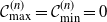$\mathcal{C}_{\max}^{(n)}=\mathcal{C}_{\min}^{(n)}=0$ . We define the $\{0,3,4,\ldots\}$ -valued random variables $\mathcal{S}$ and $\mathcal{L}$ for the limits of the shortest and longest cycle, respectively, via

\begin{equation*}\mathbb{P}(\mathcal{S}=0)=\mathbb{P}(\mathcal{L}=0)=\exp\Biggl({-}\sum_{k=3}^\infty\lambda_k\Biggr)\end{equation*}

and

\begin{equation*}\mathbb{P}(3\leq \mathcal{S} \leq t) =1-\exp\Biggl({-}\sum_{k=3}^t\lambda_k\Biggr)\end{equation*}

as well as

\begin{equation*}\mathbb{P}(\mathcal{L} \leq t)=\exp\Biggl({-}\sum_{k=t+1}^{\infty}\lambda_k\Biggr)\end{equation*}

for all $t\in\mathbb{N}_{\geq3}$ . We measure the rate of convergence in the Kolmogorov distance given by

\begin{equation*}d_{\text{Kol}}(X,Y)=\sup\nolimits_{t\in \mathbb{R}}|\mathbb{P}(X\leq t)-\mathbb{P}(Y\leq t)|\end{equation*}

for two random variables X and Y.

Relation with similar models

Theorems 2.1–2.5 also hold for the Chung–Lu model [Reference Chung and Lu10] and the (erased) Norros–Reittu model [Reference Norros and Reittu23]. The original Norros–Reittu model may produce loops, i.e. edges from a vertex to itself, and multiple edges between two vertices. In order to obtain a simple graph we erase all loops and merge multiple edges into single edges. This yields the erased Norros–Reittu model. We quickly define the models. Similarly to the generalised random graph, we take the vertices $[n]=\{1,\ldots,n\}$ equipped with i.i.d. weights $W_1,\ldots,W_n$ for $n\in\mathbb{N}$ . Conditionally on the weights, we connect any two distinct vertices $i,j\in[n]$ independently with probability

\[\mathbb{P}_{\mathcal{W},\mathit{CL}}(i\leftrightarrow j)=\min\!(1,W_iW_j/L_n) \quad\text{and}\quad \mathbb{P}_{\mathcal{W},\mathit{NR}}(i\leftrightarrow j)=1-\exp\!({-}W_iW_j/L_n)\]

in the Chung–Lu model and the erased Norros–Reittu model, respectively. If one is only interested in the qualitative results, they follow immediately from the asymptotic equivalence provided in Example 3.6 in [Reference Janson17]. If one wishes to keep quantitative results, one would need to quantify this asymptotic equivalence. We provide a simpler argument. All our proofs rely on lower and upper bounds of the connection probability

\[\mathbb{P}_\mathcal{W}(i\leftrightarrow j)=\frac{W_iW_j}{W_iW_j+L_n}\]

for two distinct vertices $i,j\in[n]$ in the generalised random graph. From $1+x\leq \exp\!(x)$ for all $x\in\mathbb{R}$ we obtain

\[\exp\!({-}x)\leq \frac{1}{1+x} \Leftrightarrow \frac{x}{1+x}=1-\frac{1}{1+x}\leq 1-\exp\!({-}x)\]

and with $x=W_iW_j/L_n$ we conclude

\begin{equation*}\frac{W_iW_j}{W_iW_j+L_n}\leq 1-\exp\biggl({-}\frac{W_iW_j}{L_n}\biggr)\leq \min\biggl(1,\frac{W_iW_j}{L_n}\biggr),\end{equation*}

where the last inequality uses $\exp\!(x)>0$ and $1-\exp\!({-}x)\leq x$ for all $x\in\mathbb{R}$ . Therefore we get

\begin{equation*}\mathbb{P}_\mathcal{W}(i\leftrightarrow j)\leq \mathbb{P}_{\mathcal{W},\mathit{NR}}(i\leftrightarrow j)\leq \mathbb{P}_{\mathcal{W},\mathit{CL}}(i\leftrightarrow j).\end{equation*}

This is also known as stochastic domination of the underlying graphs; see e.g. Section 6.8.2 in [Reference van der Hofstad14]. The inequalities above imply that the lower bound we use for the generalised random graph applies to all three models. The upper bounds we use are 1 and $W_iW_j/L_n$ and therefore also remain upper bounds for all three models. Thus the proofs and the results transfer to the Chung–Lu model and the Norros–Reittu model.

3. Results on Poisson approximation and the Poisson Cramér–Wold device

We start by providing the framework of the Poisson approximation from [Reference Arratia, Goldstein and Gordon2], but in a conditioned setting. Let I denote an arbitrary index set and $\mathcal{A}$ a $\sigma$ -field. We write $\mathbb{E}_\mathcal{A}$ as a shorthand notation for the conditional expectation with respect to $\mathcal{A}$ . For all $\alpha\in I$ , let $X_\alpha$ be a Bernoulli random variable. We are interested in the number of successes $S=\sum_{\alpha\in I}X_\alpha$ . Additionally, let $B_\alpha\subseteq I$ be such that $\alpha\in B_\alpha$ for all $\alpha\in I$ , and define

(2) \begin{align} b_1&= \sum_{\alpha\in I}\sum_{\beta\in B_\alpha}p_\alpha p_\beta & & \text{for $p_\alpha=\mathbb{E}_\mathcal{A}[X_\alpha]$,}\end{align}

(3) \begin{align}b_2&= \sum_{\alpha\in I}\sum_{\beta\in B_\alpha\setminus\{\alpha\}}p_{\alpha\beta}& &\text{for $ p_{\alpha\beta}=\mathbb{E}_\mathcal{A}[X_\alpha X_\beta]$,}\\b_3&= \sum_{\alpha\in I}\mathbb{E}_\mathcal{A}[|\mathbb{E}[X_\alpha-p_\alpha|\sigma(\mathcal{A},X_\beta\colon \beta\in B_\alpha^c)]|].\nonumber \end{align}

We denote a mixed Poisson distribution by $X\sim\operatorname{Poi}(Y)$ , meaning that the distribution of X conditionally on Y is a Poisson distribution with parameter Y. The proof of the following lemma is analogous to the proof of Theorem 1 in [Reference Arratia, Goldstein and Gordon2] and is postponed to Section 6. In the case that $\mathcal{A}$ is the trivial $\sigma$ -field, the lemma below follows from Theorem 1 in [Reference Arratia, Goldstein and Gordon2]. See also [Reference Erhardsson11] and [Reference Ross24] for more details on Stein’s method for Poisson approximation.

Lemma 3.1. If $T_\mathcal{A}\sim\operatorname{Poi}(\mathbb{E}_\mathcal{A}[S])$ , then

\begin{equation*}d_{TV}(S,T_\mathcal{A})\leq \mathbb{E}[{\min}(1,b_{1}+b_{2}+b_{3})].\end{equation*}

From this lemma we deduce the following statement. Its short proof is also in Section 6.

Lemma 3.2. For $Z\sim\operatorname{Poi}(\mu)$ with $\mu>0$ ,

\begin{equation*}d_{TV}(S,Z)\leq \mathbb{E}[{\min}(1,b_1+b_2+b_3)]+\mathbb{E}[{\min}(1,|\mathbb{E}_\mathcal{A}[S]-\mu|)].\end{equation*}

We wish to add a brief comment on the benefit of having the conditional version. Here it suffices to show $b_1+b_2+b_3\to0$ and $|\mathbb{E}_\mathcal{A}[S]-\mu|\to 0$ in probability as $n\to\infty$ to obtain a qualitative, albeit not quantitative result. This allows us to get rid of the additional assumption $\mathbb{E}[W^4]<\infty$ required for the quantitative result in Theorem 2.2.

We present the choices for I, $X_\alpha$ , and $B_\alpha$ in our setting. For any set D and $k\in\mathbb{N}$ , we write $D^k_{\neq}$ for the k-tuples with pairwise distinct entries from D. For $k\in\mathbb{N}_{\geq3}$ and $n\in\mathbb{N}$ let

\begin{equation*}I_k=I_k(n)=\Bigl\{\alpha\in[n]^k_{\neq}\colon \alpha_1=\min_{i=1,\ldots,k}\alpha_i,\alpha_2<\alpha_k\Bigr\},\end{equation*}

which represents the possible cycles of length k. The constraints on $\alpha$ in $I_k$ correspond to fixing a starting vertex $\alpha_1$ and an orientation of the cycle $\alpha$ to ensure that each cycle corresponds to exactly one $\alpha\in I_k$ . We suppress the dependence of $I_k$ on n in the notation for simplicity. In this work we study $\mathcal{C}_n(A)$ , the number of cycles whose length lies in some set $A\subseteq\mathbb{N}_{\geq3}$ . For $k\in\mathbb{N}_{\geq3}$ and $\alpha\in I_k$ , we write

(4) \begin{equation}X_\alpha=\boldsymbol{1}\{\text{the cycle }\alpha\text{ exists} \}=\boldsymbol{1}\{\alpha_1\leftrightarrow\alpha_2\leftrightarrow\cdots\leftrightarrow \alpha_k\leftrightarrow\alpha_1\}, \end{equation}

so that we have

\begin{equation*}\mathcal{C}_n(A)=\sum_{k\in A}\sum_{\alpha\in I_k}X_\alpha=\sum_{\alpha\in I}X_\alpha\quad\text{for}\ I=\bigcup_{k\in A}I_k.\end{equation*}

For $A\subseteq \mathbb{N}_{\geq3}$ and $\alpha\in I$ the choice of $B_\alpha$ will differ in Sections 4 and 5. The reason is a different choice of the $\sigma$ -field $\mathcal{A}$ . In Section 4, i.e. for Theorem 2.1, we choose $\mathcal{A}=\mathcal{W}$ . Conditionally on the weights, the random variables $X_\beta,\beta\in I$ , are independent as soon as they share no edges. Choosing

(5) \begin{equation}B_\alpha=B_\alpha(n)=\{\beta\in I\colon \alpha \text{ and }\beta \text{ share at least one edge}\} \end{equation}

therefore ensures that $b_3=0$ for this choice of $\mathcal{A}$ . In Section 5 we choose $\mathcal{A}$ as the trivial $\sigma$ -field instead. If we were to choose $B_\alpha$ as above, then $b_3$ no longer needs to be zero as $X_\alpha$ and $X_\beta$ corresponding to two cycles with at least one shared vertex are not independent due to the weight of that vertex. This is why we choose

(6) \begin{equation}B_{\alpha}=B_\alpha(n)=\{\beta\in I\colon \alpha \text{ and }\beta \text{ share at least one vertex}\} \end{equation}

instead, which once more results in $b_3=0$ .

Next, we provide a corollary to the so-called Poisson Cramér–Wold device. We use this tool to establish the finite-dimensional convergence equivalent to the claim in Theorem 2.1. A two-dimensional version of the statement can be found in Corollary 2.3 in [Reference Angel, van der Hofstad and Holmgren1]. The two-dimensional proof generalises to higher dimensions.

For $m\in\mathbb{N}$ and $\mathbb{N}_0$ -valued random variables $Y_1,\ldots,Y_m$ as well as $q_1,\ldots,q_m\in[0,1]$ , let

\begin{equation*}Y_i^{(q_i)}\sim\textrm{Bin}(Y_i,q_i) \quad \text{for $i=1,\ldots,m$,}\end{equation*}

where 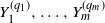$Y_1^{(q_1)},\ldots,Y_m^{(q_m)}$ are independent, conditionally on $Y_1,\ldots,Y_m$ . This is referred to as thinning.

Corollary 3.1. Let $(\boldsymbol{Y}_n=(Y_{1,n},\ldots,Y_{m,n}))_{n\in\mathbb{N}}$ be a sequence of $\mathbb{N}_0^m$ -valued random variables. Suppose that there are $\mu_1,\ldots,\mu_m>0$ such that for all $q=(q_1,\ldots,q_m)\in[0,1]^m,$

\begin{equation*}\sum_{i=1}^mY_{i,n}^{(q_i)}\overset{d}{\longrightarrow} Y_{q,\mu}\sim\operatorname{Poi}\Biggl(\sum_{i=1}^mq_i\mu_i\Biggr)\quad\ as\ \text{$n\to\infty$.}\end{equation*}

Then

\begin{equation*}\boldsymbol{Y}_n\overset{d}{\longrightarrow}\boldsymbol{Y}\sim\otimes_{i=1}^m\operatorname{Poi}(\mu_i) \quad\ as\ \text{$n\to\infty$.}\end{equation*}

4. Proof of Theorem 2.1

The following lemma is a direct consequence of the Marcinkiewicz–Zygmund strong law of large numbers; see e.g. Theorem 5.23 in [Reference Kallenberg20].

Lemma 4.1. Suppose that $\mathbb{E}[W^2]<\infty$ . For all $\gamma,\vartheta>1$ with $\gamma/\vartheta\leq 2$ ,

\[n^{-\vartheta}\sum_{i=1}^nW_i^{\gamma}\overset{\textit{a.s.}}{\longrightarrow}0\quad\ as\ \text{$n\to\infty$.}\]

We also employ the following inequality from Lemma 8 in [Reference Liu, Dong and Wang22], which can be proved via induction.

Lemma 4.2. For $k\in\mathbb{N}$ and $b,x_1,\ldots,x_k\in(0,\infty)$ , we have

\begin{equation*}\prod_{i=1}^k\frac{1}{b+x_i}\geq \frac{1}{b^k}-\frac{\sum_{i=1}^kx_i}{b^{k+1}}.\end{equation*}

Proof of Theorem 2.1. As mentioned before Theorem 2.1, the claimed convergence is equivalent to convergence of the finite-dimensional distributions. Thus we let $A\subseteq\mathbb{N}_{\geq 3}$ be finite. By the Poisson Cramér–Wold device, Corollary 3.1, it suffices to show for $q_k\in[0,1]$ for $k\in A$ that

\[\sum_{k\in A}\mathcal{C}_n^{(q_k)}(k)=\sum_{k\in A}\sum_{\alpha \in I_k}X_{\alpha}^{(q_k)}\overset{d}{\longrightarrow}Z\sim \operatorname{Poi}\Biggl(\sum_{k\in A}q_k\lambda_k\Biggr)\quad\text{as $n\to\infty$.}\]

We use the notation from Section 3, $\mathcal{A}=\mathcal{W}$ , and the choice for $B_\alpha$ in (5). Note that $X_\alpha^{(q_k)}$ is still a Bernoulli random variable so the results from the previous section are applicable. By Lemma 3.2 it suffices to show that $b_1,b_2,b_3$ , and

(7) \begin{equation}\Biggl|\mathbb{E}_\mathcal{W}\Biggl[\sum_{k\in A}\mathcal{C}_n^{(q_k)}(k)\Biggr]-\sum_{k\in A}q_k\lambda_k\Biggr|\end{equation}

converge in probability to zero as $n\to\infty$ . As argued after (5), we have $b_3=0$ . With

\begin{equation*}\mathbb{P}_\mathcal{W}(x\leftrightarrow y)=\frac{W_xW_y}{L_n+W_xW_y}\leq \frac{W_xW_y}{L_n}\end{equation*}

for distinct $x,y\in [n]$ , we conclude that

\begin{equation*}\mathbb{E}_\mathcal{W}[X_\alpha]=\mathbb{E}_\mathcal{W}\Biggl[\prod_{i=1}^k \boldsymbol{1}\{\alpha_i\leftrightarrow\alpha_{i-1}\}\Biggr]\leq \prod_{i=1}^k\frac{W_{\alpha_i}^2}{L_n}\end{equation*}

for $\alpha\in I_k$ and $k\in A$ , where we wrote $\alpha_0=\alpha_k$ . We obtain

\begin{align*}b_1&=\sum_{k,\ell\in A} \sum_{\alpha \in I_k}\sum_{\beta\in B_\alpha\cap I_\ell}\mathbb{E}_\mathcal{W}\bigl[X_\alpha^{(q_k)}\bigr]\mathbb{E}_\mathcal{W}\bigl[X_\beta^{(q_\ell)}\bigr]\\&\leq \sum_{k,\ell\in A} \sum_{\alpha \in I_k}\sum_{\beta\in B_\alpha\cap I_\ell}\mathbb{E}_\mathcal{W}[X_\alpha]\mathbb{E}_\mathcal{W}[X_\beta] \\&\leq\sum_{k,\ell\in A}\sum_{\alpha\in I_k}\sum_{\beta\in I_\ell}\boldsymbol{1}\{\alpha\text{ and } \beta\text{ share an edge}\}\prod_{i=1}^k\frac{W_{\alpha_i}^2}{L_n}\prod_{j=1}^\ell\frac{W_{\beta_i}^2}{L_n},\end{align*}

by the definition of $B_\alpha$ . If $\alpha\in I_k$ and $\beta\in I_\ell$ share an edge, the weights of the two adjacent vertices appear with a fourth power in the product above. Since all cycles belong to exactly one element of I, we may assume without loss of generality that $(\alpha_1,\alpha_2)=(\beta_1,\beta_2)$ by changing the enumerations of $\alpha$ and $\beta$ . Writing 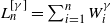$L_n^{[\gamma]}=\sum_{i=1}^nW_i^\gamma$ , we obtain

\begin{align*}b_1&\leq \sum_{k,\ell\in A}\sum_{\alpha_1,\alpha_2\in [n]}\frac{W_{\alpha_1}^4W_{\alpha_2}^4}{L_n^4}\sum_{\alpha_3,\ldots,\alpha_k\in[n]}\sum_{\beta_3,\ldots,\beta_\ell\in [n]}\prod_{i=3}^k \frac{W_{\alpha_i}^2}{L_n}\prod_{j=3}^\ell \frac{W_{\beta_j}^2}{L_n}\\&=\biggl(\frac{L_n^{[4]}}{L_n^2}\biggr)^2\sum_{k,\ell\in A}\biggl(\frac{L_n^{[2]}}{L_n}\biggr)^{k+\ell-4}\\&=\biggl(\frac{n^{-2}L_n^{[4]}}{(n^{-1}L_n)^2}\biggr)^2\sum_{k,\ell\in A}\biggl(\frac{L_n^{[2]}}{L_n}\biggr)^{k+\ell-4}.\end{align*}

The sum is almost surely bounded due to the strong law of large numbers and $\mathbb{E}[W^2]<\infty$ . Additionally, we apply Lemma 4.1 to obtain that the numerator of the first fraction tends almost surely to zero as $n\to\infty$ . The strong law of large numbers yields that the denominator converges almost surely to $\mathbb{E}[W]^2$ as $n\to\infty$ . Therefore the whole fraction converges almost surely to zero as $n\to\infty$ . In the following, we will simply refer to Lemma 4.1 for expressions similar to the first factor on the left-hand side of the equation above. For

(8) \begin{equation}b_2=\sum_{k,\ell\in A}\sum_{\alpha\in I_k}\sum_{\beta\in B_\alpha\cap I_\ell\setminus\{\alpha\}}\mathbb{E}_\mathcal{W}\bigl[X_\alpha^{(q_k)}X_\beta^{(q_\ell)}\bigr]\leq \sum_{k,\ell\in A}\sum_{\alpha\in I_k}\sum_{\beta\in B_\alpha\cap I_\ell\setminus\{\alpha\}}\mathbb{E}_\mathcal{W}[X_\alpha X_\beta],\end{equation}

we need to account for dependences between $X_\alpha$ and $X_\beta$ . For $\alpha\in I_k$ and $\beta\in B_\alpha\cap I_\ell\setminus\{\alpha\}$ , we look at the graph union $\alpha\cup\beta$ , where we take the union of the respective vertex and edge sets. This graph is given by $\alpha$ and some additional connections between vertices of $\alpha$ induced by $\beta$ . We call these connections arcs. They are paths whose two endpoints belong to $\alpha$ and whose edges and inner points belong to $\beta$ but not to $\alpha$ . We denote the number of such arcs by $m=m(\alpha,\beta)$ , which is bounded by $k/2$ and $\ell/2$ as both endpoints of an arc belong to $\alpha$ and $\beta$ . The numbers of edges of the arcs are denoted by $i_1,\ldots,i_m$ , where we enumerate the arcs in the order that one passes through them according to the labelling of $\beta$ . It follows that $1\leq i_1,\ldots,i_m\leq \ell-1$ . Note that we can reconstruct $\beta$ from $\alpha$ and the arcs so we may sum over all possibilities for the arcs instead of summing over the respective choices for $\beta$ . We use the fact that the existence of the edges of $\alpha$ and of the arcs are, conditionally on the weights, independent. The conditional expectation of the number of paths having i edges with two fixed endpoints $\alpha_s$ and $\alpha_t$ is bounded by

\begin{equation*}\frac{W_{\alpha_s}W_{\alpha_t}}{L_n}\biggl(\frac{L_n^{[2]}}{L_n}\biggr)^{i-1}\leq \frac{W_{(n)}^2}{L_n}\biggl(\frac{L_n^{[2]}}{L_n}\biggr)^{i-1},\end{equation*}

due to summing over all choices for the $i-1$ vertices in between and writing $W_{(n)}=\max_{i\in[n]}W_i$ . By summing over possible lengths, the contribution of all arcs is thus bounded by

\begin{equation*}Y_{k,\ell}\colon= \sum_{m=1}^{\min\!(k,\ell)/2}(k)_{2m}\biggl(\frac{W_{(n)}^2}{L_n}\biggr)^{m}\sum_{i_1,\ldots,i_m=1}^{\ell-1}\prod_{j=1}^{m}\biggl(\frac{L_n^{[2]}}{L_n}\biggr)^{i_j-1},\end{equation*}

where the factor $(k)_{2m}=k\cdot\,\unicode{x2026}\,\cdot(k-2m+1)$ accounts for the possibilities for choosing the endpoints of the arcs among $\alpha$ . We find for $\varepsilon>0$ that

\[\mathbb{P}\bigl(W_{(n)}^2>n\varepsilon\bigr)\leq n\mathbb{P}(W^2>n\varepsilon)\to0\quad \text{as $n\to\infty$,}\]

since $\mathbb{E}[W^2]<\infty$ implies $\mathbb{P}(W^2>t)={\textrm{o}}(1/t)$ for $t\to\infty$ . Therefore

\[\frac{W_{(n)}^2}{L_n}=\frac{W_{(n)}^2}{n}\frac{n}{L_n}\overset{\mathbb{P}}{\longrightarrow}0\]

as $n\to\infty$ , by the weak law of large numbers. This shows that $Y_{k,\ell}$ converges in probability to 0 as $n\to\infty$ for all $k,\ell\in A$ , as all sums are finite. From (8) we derive

\begin{equation*}b_2 \leq \sum_{k,\ell\in A}\sum_{\alpha\in I_k}\mathbb{E}_\mathcal{W}[X_\alpha] Y_{k,\ell} \leq\sum_{k,\ell\in A}\sum_{\alpha\in[n]_{\neq}^k}\prod_{j=1}^k\frac{W_{\alpha_j}^2}{L_n}Y_{k,\ell}\leq \sum_{k,\ell\in A}\biggl(\frac{L_n^{[2]}}{L_n}\biggr)^kY_{k,\ell}\overset{\mathbb{P}}{\longrightarrow}0\end{equation*}

as $n\to\infty$ , since A is a finite set.

For the remaining term in (7) we use the triangle inequality to deduce

\begin{equation*}\Bigg|\mathbb{E}_\mathcal{W}\Biggl[\sum_{k\in A}\mathcal{C}_n^{(q_k)}(k)\Biggr]-\sum_{k\in A}q_k\lambda_k\Bigg|\leq \sum_{k\in A} \big|\mathbb{E}_\mathcal{W}\bigl[\mathcal{C}_n^{(q_k)}(k)\bigr]-q_k\lambda_k\big|.\end{equation*}

We show for fixed $k\in A$ that the summand on the right-hand side converges almost surely to zero as $n\to\infty$ . We have

\begin{equation*}\mathbb{E}_\mathcal{W}\bigl[\mathcal{C}_n^{(q_k)}(k)\bigr]=\mathbb{E}_\mathcal{W}\Biggl[\sum_{\alpha\in I_k}X_\alpha^{(q_k)}\Biggr]=q_k\sum_{\alpha\in I_k}\mathbb{E}_\mathcal{W}[X_\alpha]=\frac{q_k}{2k}\sum_{\alpha\in[n]^k_{\neq}}\prod_{i=1}^k\frac{W_{\alpha_i^2}}{L_n+W_{\alpha_i}W_{\alpha_{i-1}}},\end{equation*}

where the factor 2k makes up for starting vertex and orientation when labelling a fixed cycle, and we write $\alpha_0=\alpha_k$ as usual. We obtain

(9) \begin{align}\frac{2k}{q_k}\mathbb{E}_\mathcal{W}\bigl[\mathcal{C}_n^{(q_k)}(k)\bigr]&=\sum_{\alpha\in[n]^k}\prod_{i=1}^k\frac{W_{\alpha_i}^2}{L_n+W_{\alpha_i}W_{\alpha_{i+1}}}\notag \\&\quad -\sum_{\alpha\in[n]^k}\boldsymbol{1}\{\exists i\neq j\colon \alpha_i=\alpha_j\}\prod_{i=1}^k\frac{W_{\alpha_i}^2}{L_n+W_{\alpha_i}W_{\alpha_{i+1}}},\end{align}

where the absolute value of the second summand is bounded by

\begin{equation*}\binom{k}{2}\frac{L_n^{[4]}}{L_n^2}\biggl(\frac{L_n^{[2]}}{L_n}\biggr)^{k-2}\end{equation*}

by choosing two of the k vertices to be equal. By Lemma 4.1 this converges almost surely to zero as $n\to\infty$ . The first summand on the right-hand side in (9) is upper-bounded by

\begin{equation*}\sum_{\alpha\in[n]^k}\prod_{i=1}^k\frac{W_{\alpha_i}^2}{L_n}=\biggl(\frac{L_n^{[2]}}{L_n}\biggr)^k\overset{\textrm{a.s.}}{\longrightarrow}\biggl(\frac{\mathbb{E}[W^2]}{\mathbb{E}[W]}\biggr)^k=2k\lambda_k.\end{equation*}

For a lower bound of the first summand on the right-hand side in (9) we use Lemma 4.2 with $b=L_n$ and $x_i=W_{\alpha_i}W_{\alpha_{i-1}}$ . This yields the lower bound

\begin{align*}\sum_{\alpha\in[n]^k}\prod_{i=1}^k\frac{W_{\alpha_i}^2}{L_n}-\sum_{\alpha\in[n]^k}\frac{\prod_{i=1}^kW_{\alpha_i}^2\sum_{j=1}^kW_{\alpha_j}W_{\alpha_{j-1}}}{L_n^{k+1}} =\biggl(\frac{L_n^{[2]}}{L_n}\biggr)^k-k\biggl(\frac{L_n^{[3]}}{L_n^{3/2}}\biggr)^2\biggl(\frac{L_n^{[2]}}{L_n}\biggr)^{k-2}.\end{align*}

As above, the last summand goes almost surely to zero as $n\to\infty$ whereas the first summand converges almost surely to $2k\lambda_k$ as $n\to\infty$ . Altogether, we obtain from (9) that

\begin{equation*}\mathbb{E}_\mathcal{W}\bigl[\mathcal{C}_n^{(q_k)}(k)\bigr]\overset{\text{a.s.}}{\longrightarrow}q_k \lambda_k\end{equation*}

as $n\to\infty$ , which concludes the proof.

5. Proofs of the quantitative theorems

Recall that we use the trivial $\sigma$ -field for $\mathcal{A}$ in this section, i.e. $\mathbb{E}_\mathcal{A}$ reduces to expectation so that e.g. $p_\alpha=\mathbb{E}[X_\alpha]$ . Also, contrary to the previous section, we use (6) as the definition for $B_\alpha$ .

5.1. Technical lemmas

In Section 3 we defined for $k,\ell\in\mathbb{N}_{\geq 3}$ and $\alpha\in I_k,\beta\in I_\ell$ the quantities $p_\alpha$ and $p_{\alpha\beta}$ ; see (2), (3), and (4). Since $p_\alpha$ , the probability of the existence of the cycle $\alpha$ having k vertices only depends on k (and n, which we suppress in our notation) but not on the exact choice of $\alpha$ , we may write $p_k=p_\alpha$ . The term $p_{\alpha\beta}$ , the probability for the existence of the two cycles $\alpha$ and $\beta$ of lengths k and $\ell$ respectively, in turn depends on the relation of $\alpha$ and $\beta$ . If they share edges, we obtain dependences between the existence of $\alpha$ and the existence of $\beta$ , even after conditioning on the weights. Therefore we need to investigate the structure of $\alpha\cap\beta$ . For a cycle $\alpha\in I_k$ we refer to its indices here and in the following always modulo k, e.g. $\alpha_{k+2}=\alpha_2$ . We introduce segments, which correspond to the parts of $\alpha$ and $\beta$ consisting of consecutively shared vertices. For $k,\ell\geq3$ and two cycles $\alpha=(\alpha_1,\ldots,\alpha_k)$ and $\beta=(\beta_1,\ldots,\beta_\ell)$ let $i\in[k],j\in[\ell]$ be such that $\alpha_i=\beta_j$ but $\alpha_{i-1}\neq\beta_{j-1},\beta_{j+1}$ . Now take $m\in[k]$ maximal with the property $\alpha_{i+1}=\beta_{j+1},\ldots,\alpha_{i+m}=\beta_{j+m}$ or $\alpha_{i+1}=\beta_{j-1},\ldots,\alpha_{i+m}=\beta_{j-m}$ so that $\alpha_i,\ldots,\alpha_{i+m}$ are consecutively shared vertices of $\alpha$ and $\beta$ . We call $(\alpha_i,\ldots,\alpha_{i+m})$ a segment of length $m+1$ . Note that segments are maximal in the sense that they cannot be extended in either direction. For instance, the two cycles $\alpha=(1,2,3,4,5,6)$ and $\beta=(2,3,6,7,1)$ share exactly two segments, the segment (1,2,3) of length 3 and the segment (6) of length 1. For two cycles $\alpha\in I_k,\beta\in I_\ell$ that intersect each other in s segments of lengths $i_1,\ldots,i_s$ we write $p_{k,\ell,s,i}=p_{\alpha\beta}$ . This is well-defined. Finally, we denote the falling factorial by $(n)_k=n\cdot\,\unicode{x2026}\cdot(n-k+1)$ for $n,k\in\mathbb{N}$ .

Lemma 5.1. Let $n\in\mathbb{N}$ and $A\subseteq\{3,\ldots,n\}$ . For $Z\sim\operatorname{Poi}(\sum_{k\in A}\lambda_k)$ ,

\begin{align*}d_{TV}(\mathcal{C}_n(A),Z)&\leq \frac{1}{2n}\sum_{k,\ell\in A}p_kp_\ell n^{k+\ell}+\sum_{k,\ell\in A}\sum_{s=1}^k\sum_{i\in [k]^s}p_{k,\ell,s,i}(2k\ell)^{s-1}n^{k+\ell-|i|}\\&\quad +\sum_{k\in A}\bigg|\frac{(n)_k}{2k}p_k-\lambda_k\bigg|.\end{align*}

Proof. We have

\begin{equation*}\mathbb{E}[\mathcal{C}_n(A)]=\sum_{k\in A}\sum_{\alpha\in I_k}\mathbb{E}[X_\alpha]=\sum_{k\in A}\sum_{\alpha\in I_k}\mathbb{E}[X_\alpha]=\sum_{k\in A}\frac{(n)_k}{2k}p_k,\end{equation*}

where we used $|I_k|=(n)_k/(2k)$ . Thus Lemma 3.2 yields

\begin{equation*}d_{TV}(\mathcal{C}_n(A),Z)\leq b_1+b_2+b_3+\sum_{k\in A}\bigg|\frac{(n)_k}{2k}p_k-\lambda_k\bigg|.\end{equation*}

We first note that $b_3=0$ by the definition of $B_\alpha$ in (6) and the brief comment thereafter. It remains to bound $b_1$ and $b_2$ . We compute

\begin{equation*}b_1 = \sum_{k,\ell\in A}\sum_{\alpha\in I_k} \sum_{\beta\in B_\alpha\cap I_\ell}\mathbb{E}[X_\alpha] \mathbb{E}[X_\beta]=\sum_{k,\ell\in A} p_k p_\ell \sum_{\alpha\in I_k} |B_\alpha\cap I_\ell|.\end{equation*}

To estimate the cardinalities of the sets, recall that $B_\alpha$ contains all cycles that intersect $\alpha\in I_k$ in at least one vertex. We have k choices for a vertex of $\alpha$ which fixes one vertex of $\beta\in B_\alpha\cap I_\ell$ . For the remaining ones, there are fewer than $n^{\ell-1}$ choices. With $|I_k|\leq n^k/(2k)$ we derive

\begin{equation*}b_1\leq \sum_{k,\ell\in A}p_kp_\ell \frac{n^k}{2k}kn^{\ell-1}=\frac{1}{2n}\sum_{k,\ell\in A}p_kp_\ell n^{k+\ell},\end{equation*}

which is the first summand on the right-hand side of the claimed inequality. Additionally,

\begin{equation*}b_2 = \sum_{k,\ell\in A}\sum_{\alpha\in I_k}\sum_{\beta\in I_\ell\cap B_\alpha\setminus\{\alpha\}}\mathbb{E}[X_\alpha X_\beta]\leq 2\sum_{k,\ell\in A\colon k\leq \ell}\sum_{\alpha\in I_k}\sum_{\beta\in I_\ell\cap B_\alpha\setminus\{\alpha\}}\mathbb{E}[X_\alpha X_\beta].\end{equation*}

The value of $\mathbb{E}[X_\alpha X_\beta]$ depends on a more thorough analysis of the intersections of $\alpha$ and $\beta$ . Recall the notion of a segment introduced above. Two distinct cycles $\alpha$ and $\beta$ may share several segments, i.e. there are maximal sequences of vertices $v_1\leftrightarrow v_2\leftrightarrow \cdots \leftrightarrow v_i$ connected by edges which are contained in the two cycles $\alpha$ and $\beta$ . For $k,\ell\in A$ with $k\leq \ell$ , $\alpha\in I_k$ and $\beta\in B_\alpha\cap I_\ell\setminus\{\alpha\}$ there can be at most $s=1,\ldots,k$ of these segments. The case $s=0$ is excluded since the two cycles share at least one vertex. We denote the number of vertices of the segments by $1\leq i_1,\ldots,i_s\leq k$ and write $i=(i_1,\ldots,i_s)$ . We define

\begin{equation*}M(s,i,\alpha)=\Biggl\{\beta\in \bigcup_{\ell\in A}I_\ell\colon \text{$\alpha$ and $\beta$ share $s$ segments of lengths $i_1,\ldots,i_s $ in that order}\Biggr\},\end{equation*}

where we order the segments with respect to the enumeration of $\alpha$ . We derive

\begin{align*}b_2&\leq 2 \sum_{k,\ell\in A\colon k\leq \ell}\sum_{\alpha\in I_k}\sum_{\beta\in I_\ell\cap B_\alpha\setminus\{\alpha\}}\sum_{s=1}^k\sum_{i\in[k]^s}\boldsymbol{1}\{\beta\in M(s,i,\alpha)\}\mathbb{E}[X_\alpha X_\beta]\\&\leq 2\sum_{k,\ell\in A\colon k\leq \ell}\sum_{\alpha\in I_k}\sum_{s=1}^k\sum_{i\in[k]^s}|B_\alpha \cap I_\ell \cap M(s,i,\alpha)|p_{k,\ell,s,i}.\end{align*}

For $k,\ell\in A$ with $k\leq \ell$ as well as $\alpha\in I_k,s\in[k]$ and $i\in[k]^s$ we bound the cardinality of $B_\alpha\cap I_\ell\cap M(s,i,\alpha)$ . We write $|i|=\sum_{j=1}^si_j$ for the total number of shared vertices. Since $\alpha=(\alpha_1,\ldots,\alpha_k)\in I_k$ has a fixed order, we may talk about the first vertex of a segment, i.e. the endpoint $\alpha_j$ of the segment with minimal j among the two endpoints. There are at most $k^s$ possibilities for choosing the first vertices of the s segments among the k vertices of $\alpha$ , call them $v_1,\ldots,v_s$ . We may assume without loss of generality that $v_1$ is the first entry of $\beta=(\beta_1,\ldots,\beta_\ell)$ . This leaves us with placing the $s-1$ remaining vertices $v_2,\ldots,v_s$ among the $\ell-1$ remaining slots in $\beta$ , giving us fewer than $\ell^{s-1}$ choices. We need to decide whether $v_j$ is the first or the last vertex of the jth segment with respect to the orientation of $\beta$ . This gives us another factor $2^{s-1}$ because we may assume that the orientation of $\beta$ coincides with the orientation of the first segment. This determines the $|i|$ entries of $\beta$ that also belong to $\alpha$ . Finally, we fill the remaining $\ell-|i|$ entries of $\beta$ , amounting to fewer than $n^{\ell-|i|}$ choices. In total we obtain

\begin{align*}b_2 &\leq 2\sum_{k,\ell\in A\colon k\leq \ell}\sum_{\alpha\in I_k}\sum_{s=1}^k\sum_{i\in[k]^s}k^s\ell^{s-1}2^{s-1}n^{\ell-|i|}p_{k,\ell,s,i}\\&\leq 2\sum_{k,\ell\in A}\frac{n^k}{2k}\sum_{s=1}^k\sum_{i\in[k]^s}k^s\ell^{s-1}2^{s-1}n^{\ell-|i|}p_{k,\ell,s,i}\\&=\sum_{k,\ell\in A}\sum_{s=1}^k\sum_{i\in[k]^s}(2k\ell)^{s-1}n^{k+\ell-|i|}p_{k,\ell,s,i},\end{align*}

which concludes the proof.

The next lemma is a special case of Lemma 1 in [Reference Bobkov, Danshina and Ulyanov6]. It is some variant of the Chernoff bound for random variables with finite second moments.

Lemma 5.2. Let $n\in\mathbb{N}$ and $Y_1,\ldots,Y_n$ be non-negative i.i.d. random variables with $\mathbb{E}[Y_1^2]<\infty$ . For all $0<\lambda<1$ there exists a constant $c>0$ depending only on $\lambda$ and the first and second moment of Y such that

\begin{equation*}\mathbb{P}\Biggl(\sum_{i=1}^nY_i\leq \lambda \mathbb{E}[Y_1]n\Biggr)\leq\exp\!({-}c n).\end{equation*}

The following three lemmas are used for the three summands in the bound of Lemma 5.1 and contain parts (a) and (b). We will use part (a) for Theorem 2.2, i.e. it corresponds to considering finitely many cycle lengths. Part (b) will be used for Theorem 2.4 and allows the considered cycles to grow logarithmically in n. We start with uniform bounds on $p_k$ .

Lemma 5.3. Suppose that $\mathbb{E}[W^2]<\infty$ .

1. (a) Let $N\in\mathbb{N}$ . There exists a constant $C>0$ which depends on N such that for all $n\in\mathbb{N},3\leq k\leq N$ ,

   \begin{equation*}p_k\leq Cn^{-k}.\end{equation*}

2. (b) Let $a>0$ and $\mathbb{E}[W^2]<\mathbb{E}[W]$ . There exists a constant $C>0$ such that for all $n\in\mathbb{N}$ and $3\leq k\leq \lfloor a\log\!(n)\rfloor $ ,

   \begin{equation*}p_k\leq Cn^{-k}.\end{equation*}

Proof. We provide a general bound, which we use for both claims. Let $3\leq k\leq n,\lambda\in(0,1),\alpha\in I_k$ and

\[A_n=\{L_n>\lambda\mathbb{E}[W]n\}.\]

Since $X_\alpha=\boldsymbol{1}\{\alpha_1\leftrightarrow \alpha_2\leftrightarrow\cdots\leftrightarrow \alpha_k\leftrightarrow \alpha_1\}$ is bounded by one, we have

\begin{equation*}p_k=p_\alpha=\mathbb{E}[X_\alpha]\leq \mathbb{P}(A_n^c)+\mathbb{E}[\boldsymbol{1}_{A_n}X_\alpha].\end{equation*}

By Lemma 5.2 we know that $\mathbb{P}(A_n^c)$ decays faster than

\[n^{-a\log\!(n)}=\exp\!({-}a\log\!(n)^2),\]

which is the fastest rate claimed in the lemma. Therefore it suffices to show that

\[\mathbb{E}[\boldsymbol{1}_{A_n}X_\alpha]\leq Dn^{-k}\]

for some constant D in the respective setting. We write $\alpha_0=\alpha_k$ . The conditional independence of distinct edges and the definition of $A_n$ yield

(10) \begin{align}\mathbb{E}[\boldsymbol{1}_{A_n}X_\alpha]&=\mathbb{E}\Biggl[\boldsymbol{1}_{A_n}\mathbb{E}_\mathcal{W}\Biggl[\prod_{i=1}^k\boldsymbol{1}\{\alpha_i\leftrightarrow\alpha_{i-1}\}\Biggr]\Biggr] \notag \\&=\mathbb{E}\Biggl[\boldsymbol{1}_{A_n}\prod_{i=1}^{k}\mathbb{P}_\mathcal{W}(\alpha_i\leftrightarrow \alpha_{i-1})\Biggr]\notag\\&=\mathbb{E}\Biggl[\boldsymbol{1}_{A_n}\prod_{i=1}^k\frac{W_{\alpha_i}W_{\alpha_{i-1}}}{L_n+W_{\alpha_i}W_{\alpha_{i-1}}}\Biggr]\notag \\&\leq \mathbb{E}\Biggl[\prod_{i=1}^k\frac{W_i^2}{\lambda\mathbb{E}[W]n}\Biggr]\notag \\&=\biggl(\frac{\mathbb{E}[W^2]}{\lambda\mathbb{E}[W]}\biggr)^kn^{-k}.\end{align}

The first claim follows by taking

\[D=\max_{k=3,\ldots,N}\biggl(\frac{\mathbb{E}[W^2]}{\lambda\mathbb{E}[W]}\biggr)^k.\]

For the second claim we choose $\lambda=\mathbb{E}[W^2]/\mathbb{E}[W]$ , which is smaller than 1 by assumption, so that $D=1$ .

The next lemma is used to bound $p_{k,\ell,s,i}$ in the second summand of Lemma 5.1.

Lemma 5.4. Suppose that $\mathbb{E}[W^4]<\infty$ .

1. (a) Let $N\in\mathbb{N}$ . There exists a constant $C>0$ which depends on N such that for all $n\in\mathbb{N},3\leq k, \ell\leq N$ and $\alpha\in I_k,\beta\in I_\ell$ which share $0\leq j\leq \min\!(k,\ell)$ edges, we have

   \begin{equation*}p_{\alpha\beta}\leq Cn^{-k-\ell+j}.\end{equation*}

2. (b) Let $a>0$ and $\mathbb{E}[W^2]<\mathbb{E}[W]$ . There exist constants $C>0,\kappa\geq 1$ such that for all $n\in\mathbb{N}$ and $3\leq k,\ell\leq \lfloor a\log\!(n) \rfloor$ and distinct $\alpha\in I_k,\beta\in I_\ell$ which intersect each other in $1\leq s\leq k$ segments of lengths $1\leq i_1,\ldots,i_s\leq \min\!(k,\ell)$ ,

   \begin{equation*}p_{k,\ell,s,i}\leq C \kappa^s n^{-k-\ell+|i|-s},\end{equation*}
   where $|i|=\sum_{j=1}^si_j$ denotes the number of all vertices that $\alpha$ and $\beta$ share.

Proof. For fixed $n\in\mathbb{N}$ and $\lambda\in(0,1)$ , we define

\[A_n=\{L_n>\lambda\mathbb{E}[W]n\}.\]

We obtain for all $3\leq k,\ell\leq n$ and $\alpha\in I_k,\beta\in I_\ell$ that

\begin{equation*}p_{\alpha\beta}=\mathbb{E}[X_\alpha X_\beta]\leq \mathbb{P}(A_n^c)+\mathbb{E}[\boldsymbol{1}_{A_n}X_\alpha X_\beta].\end{equation*}

The rates of convergence claimed in the lemma are all slower than

\[ n^{-3a\log\!(n)}= \exp\!({-}3a\log\!(n)^2).\]

By Lemma 5.2, $\mathbb{P}(A_n^c)$ decays faster. Therefore the claims follow if one can show

\[\mathbb{E}[\boldsymbol{1}_{A_n}X_\alpha X_\beta]\leq Dn^{-k-\ell+j}\quad\text{and}\quad \mathbb{E}[\boldsymbol{1}_{A_n}X_\alpha X_\beta]\leq D\kappa^sn^{-k-\ell+|i|-s}\]

respectively, for some constant $D>0$ . Write $\alpha\cup\beta$ for the graph union of the cycles induced by $\alpha$ and $\beta$ . We denote its vertices by $V(\alpha\cup\beta)$ , its edges by $E(\alpha\cup\beta)$ , and degree of $v\in V(\alpha\cup\beta)$ in $\alpha\cup\beta$ by $\deg_{\alpha\cup\beta}(v)$ . Similarly, we refer to the set of edges that belong to both $\alpha$ and $\beta$ as $E(\alpha\cap\beta)$ . We derive

\begin{align*}\mathbb{E}[\boldsymbol{1}_{A_n}X_\alpha X_\beta]& =\mathbb{E}\Biggl[\boldsymbol{1}_{A_n}\prod_{\{x,y\}\in E(\alpha\cup\beta)}\boldsymbol{1}\{x\leftrightarrow y\}\Biggr]\\&=\mathbb{E}\Biggl[\boldsymbol{1}_{A_n}\prod_{\{x,y\}\in E(\alpha\cup\beta)}\mathbb{P}_\mathcal{W}(x\leftrightarrow y)\Biggr]\\&\leq \mathbb{E}\Biggl[\boldsymbol{1}_{A_n}\prod_{\{x,y\}\in E(\alpha\cup\beta)}\frac{W_xW_y}{L_n}\Biggr]\\&\leq(\lambda\mathbb{E}[W]n)^{-|E(\alpha\cup\beta)|}\prod_{x\in V(\alpha\cup\beta)}\mathbb{E}\bigl[W_x^{\deg_{\alpha\cup\beta}(x)}\bigr].\end{align*}

We continue by showing the first claim. Suppose that there is a fixed $N\in\mathbb{N}$ with $k,\ell\leq N$ and that $\alpha$ and $\beta$ share j edges. Then $|E(\alpha\cup\beta)|=k+\ell-j\leq 2N$ and the degree of any vertex $v\in V(\alpha\cup\beta)$ must lie in $\{2,3,4\}$ . Since $|V(\alpha\cup\beta)|\leq 2N$ ,

\begin{align*}\mathbb{E}[\boldsymbol{1}_{A_n}X_\alpha X_\beta]&\leq \max\bigl(1,(\lambda\mathbb{E}[W])^{-2N}\bigr)n^{-k-\ell+j}\max\!(1,\mathbb{E}[W^2],\mathbb{E}[W^3],\mathbb{E}[W^4])^{2N}\\&=\colon Dn^{-k-\ell+j},\end{align*}

which shows the first claim.

For the second claim, one can choose $\lambda=\mathbb{E}[W^2]/\mathbb{E}[W]<1$ since $\mathbb{E}[W^2]<\mathbb{E}[W]$ . Let $a>0$ , $k,\ell\leq \lfloor a\log\!(n) \rfloor$ and $\alpha\in I_k$ and $\beta\in I_\ell$ share s segments which contain $i_1,\ldots,i_s\geq 1$ vertices. Therefore $|V(\alpha\cup\beta)|=k+\ell-|i|$ . Now we analyse how many vertices of the possible degrees 2, 3, and 4 are in $\alpha\cup\beta$ . Whenever a segment has length one, this vertex needs to have degree 4. We write $m_i(1)$ for the number of segments of length 1 so that we have $m_i(1)$ vertices of degree 4 in $\alpha\cup\beta$ . When a segment has at least length two, there will be two vertices of degree 3, namely the start- and endpoint of the segment. Here we used that $\alpha\neq\beta$ . We obtain $2(s-m_i(1))$ vertices of degree 3. The remaining $k+\ell-|i|-2s+m_i(1)$ vertices have degree 2. Finally, the number of edges is given by $|E(\alpha\cup\beta)|=k+\ell-|i|+s$ . We obtain

\begin{align*}\mathbb{E}[\boldsymbol{1}_{A_n}X_\alpha X_\beta]&\leq (n\mathbb{E}[W^2])^{-k-\ell+|i|-s}\mathbb{E}[W^4]^{m_i(1)}\mathbb{E}[W^3]^{2(s-m_i(1))}\mathbb{E}[W^2]^{k+\ell-|i|-2s+m_i(1)}\\&=\biggl(\frac{\mathbb{E}[W^4]\mathbb{E}[W^2]}{\mathbb{E}[W^3]^2}\biggr)^{m_i(1)}\biggl(\frac{\mathbb{E}[W^3]^2}{\mathbb{E}[W^2]^3}\biggr)^sn^{-k-\ell+|i|-s}\\&=\colon \gamma^{m_i(1)}\delta^{s} n^{-k-\ell+|i|-s}\\&\leq \kappa^sn^{-k-\ell+|i|-s},\end{align*}

where $\kappa=\max\!(1,\gamma)\delta$ and the last inequality uses $m_i(1)\leq s$ . The assertion follows.

The following lemma will be employed to bound the third summand in Lemma 5.1.

Lemma 5.5. Suppose that $\mathbb{E}[W^3]<\infty$ .

1. (a) Let $N\in\mathbb{N}$ . There exists a constant $C>0$ such that for all $3\leq k\leq N$ and $n\in\mathbb{N}$ ,

   \begin{equation*}\bigg|\frac{(n)_k}{2k}p_k-\lambda_k\bigg|\leq \frac{kC}{n}.\end{equation*}

2. (b) Let $a>0$ and $\mathbb{E}[W^2]<\mathbb{E}[W]$ . There exists a constant $C>0$ such that for all $n\in\mathbb{N}$ and $3\leq k\leq \lfloor a\log\!(n) \rfloor$ ,

   \begin{equation*}\bigg|\frac{(n)_k}{2k}p_k-\lambda_k\bigg|\leq \frac{kC}{n}.\end{equation*}

Proof. We provide a single proof that works for both claims with the correct parameter choices. Let $M_n=N$ for the first claim and $M_n=\lfloor a\log\!(n)\rfloor$ for the second claim and $3\leq k\leq M_n$ . We may assume without loss of generality that $M_n< n$ as $M_n={\textrm{o}}(n)$ as $n\to\infty$ . With $W_0=W_k$ ,

\begin{equation*}p_k=\mathbb{E}\Biggl[\prod_{i=1}^k\frac{W_i^2}{L_n+W_iW_{i-1}}\Biggr].\end{equation*}

We provide lower and upper bounds on $p_k$ to obtain the desired statements. For $\lambda\in(0,1)$ and $1\leq j<n$ we define $L_{n,j}=\sum_{i=j+1}^nW_i$ and

\begin{equation*}A_n= \{L_{n,M_n}>(n-M_n)\lambda\mathbb{E}[W]\},\end{equation*}

where we choose $\lambda=1/2$ for the first claim of the lemma and $\lambda=\mathbb{E}[W^2]/\mathbb{E}[W]$ for the second claim. Note that $A_n$ is independent of $W_1,\ldots,W_{k}$ . For an upper bound we compute

\begin{align*}p_k&\leq \mathbb{E}\Biggl[\prod_{i=1}^k\frac{W_i^2}{L_n}\Biggr]\\&=\mathbb{E}\Biggl[\boldsymbol{1}_{A_n}\prod_{i=1}^k\frac{W_i^2}{L_n}\Biggr]+\mathbb{E}\Biggl[\boldsymbol{1}_{A_n^c}\prod_{i=1}^k\frac{W_i^2}{L_n}\Biggr]\\&=\colon \mathbb{E}\Biggl[\boldsymbol{1}_{A_n}\prod_{i=1}^k\frac{W_i^2}{L_n}\Biggr]+\frac{2k}{(n)_k}R_1(k).\end{align*}

For a lower bound we use Lemma 4.2 with $b=L_n$ and $x_i=W_iW_{i-1}$ for $i=1,\ldots,k$ , so that

\begin{align*}p_k&=\mathbb{E}\Biggl[\prod_{i=1}^k\frac{W_i^2}{L_n+W_iW_{i-1}}\Biggr]\\&\geq \mathbb{E}\Biggl[\boldsymbol{1}_{A_n}\prod_{i=1}^k\frac{W_i^2}{L_n+W_iW_{i-1}}\Biggr]\\&\geq \mathbb{E}\Biggl[\boldsymbol{1}_{A_n}\prod_{i=1}^k\frac{W_i^2}{L_n}\Biggr]-\mathbb{E}\Biggl[\boldsymbol{1}_{A_n}\frac{1}{L_n^{k+1}}\sum_{j=1}^kW_jW_{j-1}\prod_{i=1}^kW_i^2\Biggr]\\&=\colon \mathbb{E}\Biggl[\boldsymbol{1}_{A_n}\prod_{i=1}^k\frac{W_i^2}{L_n}\Biggr]-\frac{2k}{(n)_k}R_2(k).\end{align*}

We continue by showing

(11) \begin{equation}\Bigg|\frac{(n)_k}{2k}\mathbb{E}\Biggl[\boldsymbol{1}_{A_n}\prod_{i=1}^k\frac{W_i^2}{L_n}\Biggr]-\lambda_k\Bigg|\leq\sum_{i=3}^6R_i(k)\end{equation}

with

\begin{align*}R_3(k)&=\frac{(n)_k}{2k}\mathbb{E}\Biggl[\boldsymbol{1}_{A_n}\biggl(\frac{1}{L_{n,k}^k}-\frac{1}{L_{n}^k}\biggr)\prod_{i=1}^kW_i^2\Biggr],\\R_4(k)&=(n)_k\lambda_k\mathbb{E}\Biggl[\boldsymbol{1}_{A_n}\biggl(\frac{1}{L_{n,k}^k}-\frac{1}{L_n^k}\biggr)\prod_{i=1}^kW_i\Biggr],\\R_5(k)&=(n)_k\lambda_k\mathbb{E}\Biggl[\boldsymbol{1}_{A_n^c}\prod_{i=1}^k\frac{W_i}{L_n}\Biggr],\\R_6(k)&=\lambda_k\mathbb{E}\Biggl[\sum_{v\in[n]^k_{=}}\prod_{i=1}^k\frac{W_{v_i}}{L_n}\Biggr],\end{align*}

where 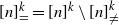$[n]^k_{=}=[n]^k\setminus[n]^k_{\neq}$ denotes the k-tuples in $[n]^k$ with at least two equal entries. After establishing (11), combining the lower and upper bound yields

\begin{equation*}\bigg|\frac{(n)_k}{2k}p_k-\lambda_k\bigg|\leq \sum_{i=1}^6R_i(k),\end{equation*}

and it remains to show the claimed bound for $R_1(k),\ldots,R_6(k)$ . We show (11) by rewriting

\begin{equation*}\frac{(n)_k}{2k}\mathbb{E}\Biggl[\boldsymbol{1}_{A_n}\prod_{i=1}^k\frac{W_i^2}{L_n}\Biggr]=\frac{(n)_k}{2k}\mathbb{E}\Biggl[\boldsymbol{1}_{A_n}\prod_{i=1}^k\frac{W_i^2}{L_{n,k}}\Biggr]-R_3(k).\end{equation*}

Because $A_n$ and $L_{n,k}$ are independent of $W_1,\ldots,W_k$ , we derive

\begin{align*}\frac{(n)_k}{2k}\mathbb{E}\Biggl[\boldsymbol{1}_{A_n}\prod_{i=1}^k\frac{W_i^2}{L_{n,k}}\Biggr]&=\frac{(n)_k}{2k}\prod_{i=1}^k\frac{\mathbb{E}[W_i^2]}{\mathbb{E}[W_i]}\times \mathbb{E}\Biggl[\boldsymbol{1}_{A_n}\prod_{j=1}^k\frac{W_j}{L_{n,k}}\Biggr]\\&=(n)_k\lambda_k\mathbb{E}\Biggl[\boldsymbol{1}_{A_n}\prod_{i=1}^k\frac{W_i}{L_{n,k}}\Biggr]\\&=(n)_k\lambda_k\mathbb{E}\Biggl[\boldsymbol{1}_{A_n}\prod_{i=1}^k\frac{W_i}{L_{n}}\Biggr]+R_4(k)\\&=(n)_k\lambda_k\mathbb{E}\Biggl[\prod_{i=1}^k\frac{W_i}{L_n}\Biggr]-R_5(k)+R_4(k).\end{align*}

Observe that $|[n]^k_{\neq}|=(n)_k$ and use $\sum_{v\in[n]^k}\prod_{i=1}^kW_{v_i}=L_n^k$ to rewrite

\begin{equation*}(n)_k\lambda_k\mathbb{E}\Biggl[\prod_{i=1}^k\frac{W_i}{L_{n}}\Biggr]=\lambda_k\mathbb{E}\Biggl[\sum_{v\in[n]^k_{\neq}}\prod_{i=1}^k\frac{W_{v_i}}{L_{n}}\Biggr]=\lambda_k-\lambda_k\mathbb{E}\Biggl[\sum_{v\in[n]^k_{=}}\prod_{i=1}^k\frac{W_{v_i}}{L_{n}}\Biggr]=\lambda_k-R_6(k).\end{equation*}

Applying the triangle inequality shows (11), and we proceed by establishing

(12) \begin{equation}R_i(k)\leq \frac{kC_i}{n} \end{equation}

for some constant $C_i>0$ and $i=1,\ldots,6$ . From Lemma 5.2 we obtain some $c>0$ with

\begin{equation*}n^{2k+1}\mathbb{P}(A_n^c)\leq n^{2M_n+1}\exp\!({-}c(n-M_n))=\exp\!((2M_n+1)\log\!(n)-cn+cM_n)\to 0\end{equation*}

as $n\to\infty$ . In particular, there exists a constant $c_A$ not depending on k and n such that

\begin{equation*}\mathbb{P}(A_n^c)\leq c_An^{-2k-1}.\end{equation*}

Using $W_i\leq L_n$ for $i=1,\ldots,n$ as well as the independence of $A_n$ and $W_1,\ldots,W_{M_n}$ , we get

\begin{equation*}R_1(k)=\frac{(n)_k}{2k}\mathbb{E}\Biggl[\boldsymbol{1}_{A_n^c}\prod_{i=1}^k\frac{W_i^2}{L_n}\Biggr]\leq n^k\mathbb{E}[W]^k\mathbb{P}(A_n^c)\leq c_A\mathbb{E}[W]^kn^{k-2k-1}= c_A\biggl(\frac{\mathbb{E}[W]}{n}\biggr)^kn^{-1},\end{equation*}

showing (12) for $i=1$ . Concerning $R_5(k)$ we obtain similarly, using the definition of $\lambda_k$ in (1),

(13) \begin{equation}R_5(k)=(n)_k\lambda_k\mathbb{E}\Biggl[\boldsymbol{1}_{A_n^c}\prod_{i=1}^k\frac{W_i}{L_n}\Biggr]\leq n^k\biggl(\frac{\mathbb{E}[W^2]}{\mathbb{E}[W]}\biggr)^k\mathbb{P}(A_n^c)\leq \biggl(\frac{\mathbb{E}[W^2]}{n\mathbb{E}[W]}\biggr)^kc_An^{-1},\end{equation}

which implies (12) for $i=5$ . Additionally, we have

(14) \begin{equation}R_6(k)=\lambda_k\mathbb{E}\Biggl[\boldsymbol{1}_{A_n}\sum_{v\in[n]^k_{=}}\prod_{i=1}^k\frac{W_{v_i}}{L_n}\Biggr]+\lambda_k\mathbb{E}\Biggl[\boldsymbol{1}_{A_n^c}\sum_{v\in[n]^k_{=}}\prod_{i=1}^k\frac{W_{v_i}}{L_n}\Biggr]. \end{equation}

For the second summand, note that the sum is bounded by one so that

\begin{equation*}\lambda_k\mathbb{E}\Biggl[\boldsymbol{1}_{A_n^c}\sum_{v\in[n]^k_{=}}\prod_{i=1}^k\frac{W_{v_i}}{L_n}\Biggr]\leq \frac{1}{2k}\biggl(\frac{\mathbb{E}[W^2]}{\mathbb{E}[W]}\biggr)^k\mathbb{P}(A_n^c),\end{equation*}

which can be bounded as in (13). For the first summand on the right-hand side in (14), there are fewer than $k^2$ choices for the indices of two equal entries of $v\in[n]^k_=$ . This gives us

\begin{equation*}\sum_{v\in[n]^k_=}\prod_{i=1}^kW_{v_i}\leq k^2\sum_{v\in[n]}W_v^2L_n^{k-2}\end{equation*}

and thus, using $A_n$ to bound $L_n$ ,

\begin{equation*}\lambda_k\mathbb{E}\Biggl[\boldsymbol{1}_{A_n}\sum_{v\in[n]^k_{=}}\prod_{i=1}^k\frac{W_{v_i}}{L_{n}}\Biggr]\leq \lambda_k k^2n\mathbb{E}\biggl[\boldsymbol{1}_{A_n}\frac{W_1^2}{L_n^2}\biggr]\leq \frac{k}{2n}\biggl(\frac{n}{n-M_n}\biggr)^2\frac{\mathbb{E}[W^2]^{k+1}}{\lambda^2\mathbb{E}[W]^{k+2}}.\end{equation*}

The second factor on the right-hand side converges to 1 as $n\to\infty$ since $M_n={\textrm{o}}(n)$ . The last term is bounded by its maximum over $k=3,\ldots,N$ in the first case. In the second case we have $\mathbb{E}[W^2]<\mathbb{E}[W]$ so that the fraction is bounded by $\lambda^{-2}/\mathbb{E}[W]$ , showing (12) for $i=6$ .

Before we continue with the remaining terms $R_2(k)$ , $R_3(k)$ , and $R_4(k)$ , we observe that the inequality $1+x\leq {\textrm{e}}^x$ for $x\in\mathbb{R}$ and $M_n^2={\textrm{o}}(n)$ imply

(15) \begin{equation}1\leq \biggl(\frac{n}{n-M_n}\biggr)^{k}\leq \biggl(\frac{n}{n-M_n}\biggr)^{M_n}=\biggl(1+\frac{M_n}{n-M_n}\biggr)^{M_n}\leq \exp\biggl(\frac{M_n^2}{n-M_n}\biggr)\to 1\end{equation}

as $n\to\infty$ . For $R_2(k)$ we again use $A_n$ to bound $L_n^{-k-1}$ and compute

(16) \begin{align}R_2(k)&=\frac{(n)_k}{2k}\mathbb{E}\Biggl[\boldsymbol{1}_{A_n}\frac{1}{L_n^{k+1}}\sum_{j=1}^kW_jW_{j-1}\prod_{i=1}^kW_i^2\Biggr]\notag \\[4pt]&\leq \frac{n^k}{2k}\frac{k\mathbb{E}[W^3]^2\mathbb{E}[W^2]^{k-2}}{((n-M_n)\lambda\mathbb{E}[W])^{k+1}}\nonumber\\[4pt]&=\frac{1}{2n}\biggl(\frac{n}{n-M_n}\biggr)^{k+1}\frac{\mathbb{E}[W^3]^2\mathbb{E}[W^2]^{k-2}}{(\lambda\mathbb{E}[W])^{k+1}}.\end{align}

By (15), the second fraction in (16) is bounded by some constant. For the third fraction we do a case distinction. For $3\leq k\leq N$ the bound is trivial by taking the maximum. In the second setting, plugging in $\lambda=\mathbb{E}[W^2]/\mathbb{E}[W]$ simplifies the expression to $\mathbb{E}[W^3]^2/\mathbb{E}[W^2]^3$ and shows (12) for $i=2$ . For $R_3(k)$ we apply the mean value theorem to $f(x)=x^{-k}$ . This gives us

\begin{equation*}\frac{1}{L_{n,k}^k}-\frac{1}{L_n^k}\leq k\sum_{j=1}^kW_jL_{n,k}^{-k-1}\end{equation*}

so that, using $A_n$ to bound $L_{n,k}^{-k-1}$ ,

\begin{align*}R_3(k)&=\frac{(n)_k}{2k}\mathbb{E}\Biggl[\boldsymbol{1}_{A_n}\biggl(\frac{1}{L_{n,k}^k}-\frac{1}{L_{n}^k}\biggr)\prod_{i=1}^kW_i^2\Biggr]\\[4pt]&\leq \frac{n^k}{2k}\mathbb{E}\Biggl[\boldsymbol{1}_{A_n}k\sum_{j=1}^kW_jL_{n,k}^{-k-1}\prod_{i=1}^kW_i^2\Biggr]\\[4pt]&\leq \frac{n^k}{2k}k^2\mathbb{E}[W^3]\mathbb{E}[W^2]^{k-1}\biggl(\frac{1}{(n-M_n)\lambda\mathbb{E}[W]}\biggr)^{k+1}\\[4pt]&=\frac{k}{2n}\biggl(\frac{n}{n-M_n}\biggr)^{k+1}\frac{\mathbb{E}[W^3]\mathbb{E}[W^2]^{k-1}}{(\lambda\mathbb{E}[W])^{k+1}}.\end{align*}

The same argument as for (16) yields (12) for $i=3$ . Similarly, we obtain for $R_4(k)$ that

\begin{align*}R_4(k)&=(n)_k\lambda_k\mathbb{E}\Biggl[\boldsymbol{1}_{A_n}\biggl(\frac{1}{L_{n,k}^k}-\frac{1}{L_n^k}\biggr)\prod_{i=1}^kW_i\Biggr]\\[4pt]&\leq \frac{n^k}{2k}\biggl(\frac{\mathbb{E}[W^2]}{\mathbb{E}[W]}\biggr)^kk^2\mathbb{E}[W^2]\mathbb{E}[W]^{k-1}\biggl(\frac{1}{(n-M_n)\lambda\mathbb{E}[W]}\biggr)^{k+1}\\[4pt]&= \frac{k}{2n}\biggl(\frac{n}{n-M_n}\biggr)^{k+1}\biggl(\frac{\mathbb{E}[W^2]}{\mathbb{E}[W]}\biggr)^{k+1}\frac{1}{\mathbb{E}[W]\lambda^{k+1}}.\end{align*}

This concludes the proof.

5.2. Proofs of the theorems

Proof of Theorem 2.2. By Lemma 5.1 we have for $A\subseteq\{3,\ldots,N\}$ ,

\begin{align*}d_{TV}(\mathcal{C}_n(A),Z)&\leq \frac{1}{2n}\sum_{k,\ell=3}^Np_kp_\ell n^{k+\ell}+\sum_{k,\ell=3}^N\sum_{s=1}^k\sum_{i\in [k]^s}p_{k,\ell,s,i}(2k\ell)^{s-1}n^{k+\ell-|i|}\\&\quad +\sum_{k=3}^N\bigg|\frac{(n)_k}{2k}p_k-\lambda_k\bigg|.\end{align*}

We show that all summands can be bounded by $C/n$ for some $C>0$ . For the third summand, part (a) of Lemma 5.5 yields the existence of some $C_1>0$ such that, for all $n\in\mathbb{N}$ ,

\begin{equation*}\sum_{k=3}^N\bigg|\frac{(n)_k}{2k}p_k-\lambda_k\bigg|\leq \sum_{k=3}^N \frac{kC_1}{n}\leq \frac{C_1N^2}{n}.\end{equation*}

Next we address the first summand. From part (a) of Lemma 5.3 we know that there exists $C_2>0$ with $p_k\leq C_2n^{-k}$ for all $3\leq k\leq N$ and $n\in\mathbb{N}$ . Therefore

\begin{equation*}\frac{1}{2n}\sum_{k,\ell=1}^Np_kp_\ell n^{k+\ell}\leq \frac{N^2C_2^2}{2n}.\end{equation*}

For the second summand, note that when $\alpha$ and $\beta$ intersect in s segments of lengths $i_1,\ldots,i_s$ they share $|i|-s$ edges. Thus part (a) of Lemma 5.4 yields the existence of some $C_3>0$ with

\begin{align*}\sum_{k,\ell=1}^N\sum_{s=1}^k\sum_{i\in [k]^s}p_{k,\ell,s,i}(2k\ell)^{s-1}n^{k+\ell-|i|}&\leq \sum_{k,\ell=1}^N\sum_{s=1}^k\sum_{i\in [k]^s}C_3n^{-k-\ell+|i|-s}(2k\ell)^{s-1}n^{k+\ell-|i|}\\&=\frac{C_3}{n} \sum_{k,\ell=1}^N \sum_{s=0}^{k-1} k^{s+1}(2kl)^{s}n^{-s},\end{align*}

where the sums are bounded in n, which concludes the proof.

Proof of Theorem 2.3. By assumption we have $\mathbb{E}[W^2]<\mathbb{E}[W]$ so that we may choose

\begin{equation*}\lambda=\frac{\mathbb{E}[W^2]+\mathbb{E}[W]}{2\mathbb{E}[W]}<1.\end{equation*}

Define $A_n=\{L_n> \lambda\mathbb{E}[W]n\}$ so that Lemma 5.2 yields a positive constant c such that

(17) \begin{align}\mathbb{P}(\mathcal{C}_n(\lfloor a\log\!(n) \rfloor+1,\ldots,n)>0)&\leq \mathbb{P}(A_n^c)+\mathbb{P}(\boldsymbol{1}_{A_n}\mathcal{C}_n(\lfloor a\log\!(n) \rfloor+1,\ldots,n)>0)\nonumber\\&\leq {\textrm{e}}^{-cn}+\sum_{k=\lfloor a\log\!(n) \rfloor+1}^n\sum_{\alpha\in I_k}\mathbb{E}[\boldsymbol{1}_{A_n}X_\alpha],\end{align}

where we used the Markov inequality for the second summand. Since the first summand decays faster than the desired order, it suffices to show the claimed bound for the second summand. With (10) we compute for $k\geq3$ and $\alpha\in I_k$

\begin{equation*}\mathbb{E}[\boldsymbol{1}_{A_n}X_\alpha]\leq n^{-k}\biggl(\frac{\mathbb{E}[W^2]}{\mathbb{E}[W]}\frac{2\mathbb{E}[W]}{\mathbb{E}[W^2]+\mathbb{E}[W]}\biggr)^k=n^{-k}\biggl(\frac{2\mathbb{E}[W^2]}{\mathbb{E}[W^2]+\mathbb{E}[W]}\biggr)^k= n^{-k} p^k,\end{equation*}

with p as in Theorem 2.3 and where $\mathbb{E}[W^2]<\mathbb{E}[W]$ yields $p<1$ . Together with $|I_k|\leq n^k $ we obtain for the second summand in (17) that

\begin{equation*}\sum_{k=\lfloor a\log\!(n) \rfloor+1}^n\sum_{\alpha\in I_k}\mathbb{E}[\boldsymbol{1}_{A_n}X_\alpha]\leq \sum_{k=\lfloor a\log\!(n) \rfloor+1}^np^k=p^{\lfloor a\log\!(n) \rfloor+1}\frac{1}{1-p}.\end{equation*}

Since $\lfloor a\log\!(n) \rfloor+1\geq a\log\!(n)$ and $p<1$ , we have

\begin{equation*}p^{\lfloor a\log\!(n) \rfloor+1}\leq p^{a\log\!(n)}= n^{\log\!(p)a},\end{equation*}

which proves the claim.

Proof of Theorem 2.4. Let

\begin{equation*}p=\frac{2\mathbb{E}[W^2]}{\mathbb{E}[W^2]+\mathbb{E}[W]} \quad \text{and}\quad \rho=\frac{\mathbb{E}[W^2]}{\mathbb{E}[W]}\end{equation*}

so that $p,\rho<1$ due to $\mathbb{E}[W^2]<\mathbb{E}[W]$ . Choose $a>0$ large enough such that

\begin{equation*}a\log\!(p)<-1\quad \text{and}\quad a\log\!(\rho)<-1.\end{equation*}

Writing $M_a=\{3,4,\ldots,\lfloor a\log\!(n)\rfloor\}$ and $\overline{M}_a=\{\lfloor a\log\!(n)\rfloor +1,\ldots\}$ , we have

(18) \begin{align}d_{TV}(\mathcal{C}_n(A),\eta(A))&\leq d_{TV}(\mathcal{C}_n(A\cap M_a),\eta(A\cap M_a))+\mathbb{P}(\mathcal{C}_n(A)\neq\mathcal{C}_n(A\cap M_a))\nonumber\\&\quad +\mathbb{P}(\eta(A)\neq \eta(A\cap M_a))\nonumber\\&=d_{TV}(\mathcal{C}_n(A\cap M_a),\eta(A\cap M_a))+\mathbb{P}(\mathcal{C}_n(\overline{M}_a)>0)+\mathbb{P}(\eta(\overline{M}_a)>0).\end{align}

For the second summand above we use Theorem 2.3 to obtain a constant $C_1>0$ with

\begin{equation*}\mathbb{P}(\mathcal{C}_n(\overline{M}_a)>0)\leq C_1n^{a\log\!(p)}\leq C_1n^{-1},\end{equation*}

by the choice of a. For the third summand the definition of $\eta$ yields

\begin{equation*}\mathbb{P}(\eta(\overline{M}_a)>0)=1-\mathbb{P}(\eta(\overline{M}_a)=0)=1-\exp\Biggl({-}\sum_{k=\lfloor a\log\!(n)\rfloor +1}^\infty \lambda_k\Biggr).\end{equation*}

We use $1-\exp\!({-}x)\leq x$ for $x\in\mathbb{R}$ and $\lambda_k=\rho^k/(2k)\leq \rho^k$ to derive

\begin{equation*}1-\exp\Biggl({-}\sum_{k=\lfloor a\log\!(n) \rfloor+1}^\infty \lambda_k\Biggr)\leq \sum_{k=\lfloor a\log\!(n) \rfloor+1}^\infty \rho^k\leq \rho^{\lfloor a\log\!(n) \rfloor+1}\sum_{k=0}^\infty \rho^k.\end{equation*}

Since $\rho<1$ , this is further bounded by

\begin{equation*}\rho^{a\log\!(n)}\frac{1}{1-\rho}=n^{a\log\!(\rho)}\frac{1}{1-\rho}\leq \frac{n^{-1}}{1-\rho},\end{equation*}

again by the choice of a. It remains to consider the first summand of (18). By Lemma 5.1 we have

\begin{align*}&d_{TV}(\mathcal{C}_n(A\cap M_a),\eta(A\cap M_a))\\&\quad \leq \frac{1}{2n}\sum_{k,\ell\in M_a}p_kp_\ell n^{k+\ell}+\sum_{k,\ell\in M_a}\sum_{s=1}^k\sum_{i\in [k]^s}p_{k,\ell,s,i}(2k\ell)^{s-1}n^{k+\ell-|i|} +\sum_{k\in M_a}\bigg|\frac{(n)_k}{2k}p_k-\lambda_k\bigg|.\end{align*}

For the third summand we apply part (b) of Lemma 5.5, which yields the existence of some constant $D_1>0$ such that for all $n\in\mathbb{N}$

\begin{equation*}\sum_{k\in M_a}\bigg|\frac{(n)_k}{2k}p_k-\lambda_k\bigg|\leq \sum_{k=3}^{\lfloor a\log\!(n) \rfloor}\frac{D_1k}{n}\leq \frac{D_1a^2\log\!(n)^2}{n}.\end{equation*}

For the first summand we use part (b) of Lemma 5.3 to obtain the existence of a constant $D_2>0$ with

\begin{equation*}\frac{1}{2n}\sum_{k,\ell\in M_a}p_kp_\ell n^{k+\ell}\leq \frac{1}{2n}\sum_{k,\ell=3}^{\lfloor a\log\!(n) \rfloor}D_2^2n^{-k-\ell}n^{k+\ell}\leq \frac{D_2^2a^2\log\!(n)^2}{2n}.\end{equation*}

Finally, for the second summand, we obtain via part (b) of Lemma 5.4 the existence of constants $D_3>0$ and $\kappa\geq 1$ such that

\begin{align*}&\sum_{k,\ell\in M_a}\sum_{s=1}^k\sum_{i\in [k]^s}p_{k,\ell,s,i}(2k\ell)^{s-1}n^{k+\ell-|i|}\\&\quad \leq \sum_{k,\ell=3}^{\lfloor a\log\!(n)\rfloor}\sum_{s=1}^k\sum_{i\in [k]^s}D_3\kappa ^sn^{-k-\ell+|i|-s}(2k\ell)^{s-1}n^{k+\ell-|i|}\\&\quad =\sum_{k,\ell=3}^{\lfloor a\log\!(n) \rfloor}\frac{D_3}{2k\ell}\sum_{s=1}^k\biggl(\frac{2k^2\ell\kappa}{n}\biggr)^s\\&\quad = \sum_{k,\ell=3}^{\lfloor a\log\!(n) \rfloor}\frac{k\kappa D_3}{n}\sum_{s=0}^{k-1}\biggl(\frac{2k^2\ell\kappa}{n}\biggr)^s\\&\quad \leq \frac{\kappa D_3}{n}a^3\log\!(n)^3\sum_{s=0}^n\biggl(\frac{2\lfloor a\log\!(n) \rfloor^3\kappa}{n}\biggr)^s,\end{align*}

where the series converges to 1 due to $\lfloor a\log\!(n) \rfloor^3/n\to0$ as $n\to\infty$ and a comparison to the geometric series. This shows the claim.

Proof of Theorem 2.5. We relate the lengths of the shortest and longest cycle, respectively, to properties of the point process $\mathcal{C}_n$ . Additionally, we express the probabilities of the limiting random variables $\mathcal{S}$ and $\mathcal{L}$ in terms of the point process $\eta$ . The claim then follows from Theorem 2.4 For the claim on the shortest cycle we compute

\begin{align*}d_{\text{Kol}}\bigl(\mathcal{C}_{\min}^{(n)},\mathcal{S} \bigr)&=\sup\nolimits_{t\in\mathbb{R}}\bigl|\mathbb{P}\bigl(\mathcal{C}_{\min}^{(n)}\leq t\bigr)-\mathbb{P}(\mathcal{S} \leq t)\bigr|\\&\leq \bigl|\mathbb{P}\bigl(\mathcal{C}_{\min}^{(n)}=0\bigr)-\mathbb{P}(\mathcal{S} =0)\bigl|+\sup\nolimits_{t\in\mathbb{N}_{\geq3}}\bigr|\mathbb{P}\bigl(3\leq \mathcal{C}_{\min}^{(n)}\leq t\bigr)-\mathbb{P}(3\leq \mathcal{S} \leq t)\bigr|.\end{align*}

We defined the shortest cycle to have length zero if and only if there is no cycle. Additionally, the shortest cycle having a length between 3 and n is equivalent to the existence of at least one cycle of that length. With the definitions of $\eta$ and $\mathcal{S}$ , the term above equals

\begin{align*}&|\mathbb{P}(\mathcal{C}_n(3,4,\ldots)=0)-\mathbb{P}(\eta(3,4,\ldots)=0)|\\&\qquad +\sup\nolimits_{t\in\mathbb{N}_{\geq3}}\mathbb{P}(\mathcal{C}_n(3,\ldots,t)>0)-\mathbb{P}(\eta(3,\ldots,t)>0)|\\&\quad \leq 2\sup\nolimits_{A\subseteq\mathbb{N}_{\geq 3}}d_{TV}(\mathcal{C}_n(A),\eta(A))\\&\quad \leq \frac{2C\log\!(n)^3}{n}\end{align*}

for some constant $C>0$ by Theorem 2.4. For the longest cycle we proceed similarly and have

\begin{align*}d_{\text{Kol}}\bigl(\mathcal{C}_{\max}^{(n)},\mathcal{L} \bigr)&=\sup\nolimits_{t\in\mathbb{R}}\bigl|\mathbb{P}\bigl(\mathcal{C}_{\max}^{(n)}\leq t\bigr)-\mathbb{P}(\mathcal{L} \leq t)\bigr|\\& \leq \bigl|\mathbb{P}\bigl(\mathcal{C}_{\max}^{(n)}=0\bigr)-\mathbb{P}(\mathcal{L} =0)\bigr|+\sup\nolimits_{t\in\mathbb{N}_{\geq3}}\bigl|\mathbb{P}\bigl(\mathcal{C}_{\max}^{(n)}>t\bigr)-\mathbb{P}(\mathcal{L}>t)\bigr|\\& =|\mathbb{P}(\mathcal{C}_n(3,4,\ldots)=0)-\mathbb{P}(\eta(3,4,\ldots)=0)|\\&\quad +\sup\nolimits_{t\in\mathbb{N}_{\geq3}}|\mathbb{P}(\mathcal{C}_n(t+1,\ldots)>0)-\mathbb{P}(\eta(t+1,\ldots)>0)|\\& \leq 2\sup\nolimits_{A\subseteq\mathbb{N}_{\geq 3}}d_{TV}(\mathcal{C}_n(A),\eta(A))\\& \leq \frac{2C\log\!(n)^3}{n},\end{align*}

which concludes the proof.

6. Proofs of Lemmas 3.1 and 3.2

Proof of Lemma 3.1. The total variation distance satisfies

\begin{equation*}d_{TV}(S,T_\mathcal{A})=\frac{1}{2}\sup\nolimits_{\|h\|_{\infty}=1}|\mathbb{E}[h(S)-h(T_\mathcal{A})]|,\end{equation*}

where the supremum runs over all functions $h\colon\mathbb{N}_0\to\mathbb{R}$ with supremum norm equal to one. Thus

\begin{align*}2d_{TV}(S,T_\mathcal{A})&=\sup\nolimits_{\|h\|_{\infty}=1}|\mathbb{E}[\mathbb{E}_\mathcal{A}[h(S)-h(T_\mathcal{A})]]|\\&\leq \mathbb{E}\bigl[\!\sup\nolimits_{\|h\|_{\infty}=1}|\mathbb{E}_\mathcal{A}[h(S)-h(T_\mathcal{A})]|\bigr]\\&= \mathbb{E}\bigl[\min\bigl(2,\sup\nolimits_{\|h\|=1}\mathbb{E}_\mathcal{A}[h(S)-h(T_\mathcal{A})]\bigr)\bigr],\end{align*}

where the last equality uses $\|h\|_{\infty}=1$ and omits the absolute value as one can choose $-h$ when the expression is negative. Now one can mimic the proof of Theorem 1 in [Reference Arratia, Goldstein and Gordon2] to bound the supremum and obtain the desired statement.

Proof of Lemma 3.2. Let $T_\mathcal{A} \sim\operatorname{Poi}(\mathbb{E}_\mathcal{A}[S])$ ; then the triangle inequality and Lemma 3.1 yield

\begin{equation*}d_{TV}(S,Z)\leq d_{TV}(S,T_\mathcal{A})+d_{TV}(T_\mathcal{A},Z)\leq \mathbb{E}[{\min}(1,b_1+b_2+b_3)]+d_{TV}(T_\mathcal{A},Z).\end{equation*}

We compute

\begin{align*}d_{TV}(T_\mathcal{A},Z)&=\sup\nolimits_{A\subseteq \mathbb{N}_0}|\mathbb{P}(T_\mathcal{A}\in A)-\mathbb{P}(Z\in A)|\\&=\sup\nolimits_{A\subseteq \mathbb{N}_0}|\mathbb{E}[\mathbb{P}_\mathcal{A}(T_\mathcal{A} \in A)-\mathbb{P}(Z\in A)]|\nonumber\\&\leq \mathbb{E}[\!\sup\nolimits_{A\subseteq \mathbb{N}_0}|\mathbb{P}_\mathcal{A}(T_\mathcal{A}\in A)-\mathbb{P}(Z\in A)|]\\&=\mathbb{E}[{\min}(1,\sup\nolimits_{A\subseteq \mathbb{N}_0}|\mathbb{P}_\mathcal{A}(T_\mathcal{A}\in A)-\mathbb{P}(Z\in A)|)].\end{align*}

Since, conditionally on $\mathcal{A}$ , $T_\mathcal{A}$ follows a Poisson distribution with parameter $\lambda_\mathcal{A}=\mathbb{E}_\mathcal{A}[S]$ and Z follows a Poisson distribution with parameter $\mu$ , we obtain for all $A\subseteq\mathbb{N}_0$

\begin{equation*}|\mathbb{P}_\mathcal{A}(T_\mathcal{A}\in A)-\mathbb{P}(Z\in A)|\leq|\lambda_\mathcal{A}-\mu|;\end{equation*}

see e.g. Example 1 in [Reference Schinazi25, Chapter 21, Section 3]. The assertion follows.