1 Introduction
Cohesion between solid particles may stem from van der Waals forces and liquid bridging, to name a few possibilities (Visser Reference Visser1989; Henthorne & Hrenya Reference Henthorne and Hrenya2012; Galvin & Benyahia Reference Galvin and Benyahia2014). When the cohesive force acting on a particle is comparable to other forces acting on the particle (e.g. the weight of the particle), particles may aggregate together to form clusters of particles called agglomerates (Castellanos Reference Castellanos2005). Aggregation can have dramatic effects on flows of particles, such as decreasing the entrainment of particles in a fluidized bed (Geldart, Harnby & Wong Reference Geldart, Harnby and Wong1984), affecting the segregation and mixing of particles (Tomas Reference Tomas2004) and many more (Tomas Reference Tomas2004; Calvert, Ghadiri & Tweedie Reference Calvert, Ghadiri and Tweedie2009; Galvin & Benyahia Reference Galvin and Benyahia2014). Empirical predictions for the entrainment rate and transport disengagement height of particles in a fluidized bed vary by many orders of magnitude (Cahyadi et al. Reference Cahyadi, Neumayer, Hrenya, Cocco and Chew2015; Chew et al. Reference Chew, Cahyadi, Hrenya, Karri and Cocco2015), even before taking cohesion into account (Motlagh et al. Reference Motlagh, Grace, Salcudean and Hrenya2014). A better physical understanding of aggregation and its effects is needed. Here, the focus is on the first-principles prediction of cohesive solids engaged in ‘rapid’ flows, i.e. dilute to moderately dense flows in which the contacts are approximately binary and instantaneous in nature, rather than the enduring and multi-contact nature of very dense flows.
The discrete element method (DEM) is one approach available for the prediction of aggregation in rapid cohesive-powder flows. In the DEM, particles are tracked individually using Newton’s second law, thereby allowing for a straightforward incorporation of cohesive forces (Mikami, Kamiya & Horio Reference Mikami, Kamiya and Horio1998). Despite its wide usage for cohesive flows (e.g. Chaudhuri et al. Reference Chaudhuri, Mehrotra, Muzzio and Tomassone2006; Anand et al. Reference Anand, Curtis, Wassgren, Hancock and Ketterhagen2009; Figueroa, Li & Mccarthy Reference Figueroa, Li and McCarthy2009; Hou, Zhou & Yu Reference Hou, Zhou and Yu2012; Galvin & Benyahia Reference Galvin and Benyahia2014; Liu et al. Reference Liu, LaMarche, Kellogg and Hrenya2016b ), the DEM has a large computational overhead compared with other modelling approaches such as continuum theory, preventing its direct application to commercial units and even most laboratory-scale flows (Fullmer & Hrenya Reference Fullmer and Hrenya2017; Cocco et al. Reference Cocco, Fullmer, Liu and Hrenya2017).
The continuum framework provides a more computationally efficient approach for the prediction of cohesive-particle flows, since the solids are treated as a continuous phase via a (single) continuity equation and momentum balance. For non-cohesive rapid flows, constitutive relations for the solids-phase stress are derived based on an analogy with dense-gas kinetic theory (Gidaspow Reference Gidaspow1994; Jackson Reference Jackson2000; Goldhirsch Reference Goldhirsch2003; Brilliantov & Pöschel Reference Brilliantov and Pöschel2010; Pannala et al.
Reference Pannala, Syamlal and O’Brien2011). These closures depend on the granular temperature
 $T_{s}$
, which is a measure of the kinetic energy associated with the deviation of particle velocities from the local mean velocity, i.e.
 $T_{s}=m_{i}\langle |\boldsymbol{v}_{i}-\boldsymbol{u}|^{2}\rangle /3$
, where
 $m_{i}$
is the mass and
 $\boldsymbol{v}_{\boldsymbol{i}}$
is the instantaneous particle velocity of species
 $i$
, and
 $\boldsymbol{u}$
is the local mass-averaged mixture velocity. (The impact of correlated particle velocities due, for example, to clustering instabilities is outside the current scope and is not considered here; interested readers are referred to the reviews of Fox (Reference Fox2014) and Fullmer & Hrenya (Reference Fullmer and Hrenya2017).) Accordingly, a granular energy balance is also required. Two main approaches have been explored to incorporate the effects of cohesion into this continuum framework. The first approach is via the solution of an algebraic force balance on an agglomerate in order to determine a single agglomerate size within a control volume (i.e. numerical grid cell) (van Wachem & Sasic Reference van Wachem and Sasic2008; Le et al.
Reference Le, Avontuur, Hounslow and Salman2009; Wang, van der Hoef & Kuipers Reference Wang, van der Hoef and Kuipers2011; Motlagh et al.
Reference Motlagh, Grace, Salcudean and Hrenya2014; Vashisth et al.
Reference Vashisth, Ahmadi Motlagh, Tebianian, Salcudean and Grace2015). The equation of continuity, and momentum and granular energy balances are then solved using the single agglomerate size associated with a given control volume. The second approach utilizes a population balance, in which a differential balance on the number density of agglomerates, with source and sink terms representing aggregation and breakage, is solved for each agglomerate size (Ramkrishna Reference Ramkrishna2000). This population balance is then solved in conjunction with the kinetic-theory-based momentum and energy balances. The population-balance approach is more rigorous than its force balance counterpart as it allows for a distribution of agglomerate sizes within a given control volume, yet it requires closures for the source and sink terms for agglomerates of different sizes. Many forms of these closures have appeared in the literature, with varying degrees of physical basis. A primary focus of this work is the determination of fundamental closures for the source and sink terms in the population-balance model.
In the population balance, the source and sink terms due to aggregation and breakage are proportional to the product of the number of particles or agglomerates undergoing aggregation or breakage (the number density of pairs) and the aggregation
 $(\unicode[STIX]{x1D6FD}(V,V^{\prime }))$
or breakage
 $(\unicode[STIX]{x1D6FC}(V,V^{\prime }))$
kernels, which represent the frequency of aggregation and breakage events normalized by the number density of pairs (i.e.
 $n(V)n(V^{\prime })$
). The aggregation and breakage kernels are expected to depend on the frequency of collisions, which can be cast in terms of the (continuum quantity) granular temperature
 $T_{s}$
. However, widely used closures for the aggregation kernel include constant kernels or kernels that include the effect of agglomerate size on the collision frequency but not the explicit effect of
 $T_{s}$
(for a review, see Cameron et al. (Reference Cameron, Wang, Immanuel and Stepanek2005)). The latter widely used closures utilize a coalescence kernel constant
 $\unicode[STIX]{x1D6FD}_{0}$
, which the aggregation kernel is directly proportional to. The aggregation kernel is typically given by the product of the constant
 $\unicode[STIX]{x1D6FD}_{0}$
and a function of (only) the volumes of the particles or agglomerates undergoing aggregation (Cameron et al.
Reference Cameron, Wang, Immanuel and Stepanek2005). This coalescence kernel constant is generally chosen empirically, and implicitly takes into account the effect of
 $T_{s}$
(assumed constant) on the collision frequency. Another, more physically based, aggregation kernel
 $\unicode[STIX]{x1D6FD}(V,V^{\prime })$
is given by the product of the collision frequency and the fraction of collisions that result in aggregation, i.e. the ‘success factor’ of aggregation
 $\unicode[STIX]{x1D713}_{a}$
(Goldschmidt Reference Goldschmidt2001; Tan et al.
Reference Tan, Goldschmidt, Boerefijn, Hounslow, Salman and Kuipers2004). Fan, Marchisio & Fox (Reference Fan, Marchisio and Fox2004) extended this form of
 $\unicode[STIX]{x1D6FD}(V,V^{\prime })$
to breakage, i.e. the product of the collision frequency and the fraction of collisions resulting in breakage
 $\unicode[STIX]{x1D713}_{b}$
. Works to date that incorporate the success factors
 $\unicode[STIX]{x1D713}_{a}$
and
 $\unicode[STIX]{x1D713}_{b}$
have defined
 $\unicode[STIX]{x1D713}_{a}$
and
 $\unicode[STIX]{x1D713}_{b}$
as a constant (Fan et al.
Reference Fan, Marchisio and Fox2004; Costa, Folch & Macedonio Reference Costa, Folch and Macedonio2010; Sen & Ramachandran Reference Sen and Ramachandran2013), an empirical fit of system parameters such as mixer shear rate in a granulator (Gantt & Gatzke Reference Gantt and Gatzke2006; Fadda et al.
Reference Fadda, Cincotti, Concas, Pisu and Cao2009) or binary (0 or 1) depending on system conditions such as binder volume fraction in a granulator, as well as cohesion properties (Calvert et al.
Reference Calvert, Ghadiri and Tweedie2009; Le et al.
Reference Le, Avontuur, Hounslow and Salman2009; Braumann, Kraft & Mort Reference Braumann, Kraft and Mort2010). An inherent assumption of these approaches is that the outcome of a collision depends on the impact velocity (i.e. the relative velocity between particles at the time of contact), consistent with previous works indicating that relatively low impact velocities lead to aggregation and high impact velocities lead to rebound or breakage (e.g. Seville, Willett & Knight Reference Seville, Willett and Knight2000; Gantt & Gatzke Reference Gantt and Gatzke2006; Donahue et al.
Reference Donahue, Davis, Kantak and Hrenya2012). However, since the distribution of individual particle impact velocities is related to the (continuum) granular temperature
 $T_{s}$
, the success factors
 $\unicode[STIX]{x1D713}_{a}$
and
 $\unicode[STIX]{x1D713}_{b}$
should also depend on
 $T_{s}$
. Only one of these works includes the dependence of
 $\unicode[STIX]{x1D713}_{a}$
on
 $T_{s}$
by setting
 $\unicode[STIX]{x1D713}_{a}=0$
when
 $T_{s}$
is above a critical value and
 $\unicode[STIX]{x1D713}_{a}=1$
when
 $T_{s}$
is below a critical value (Braumann et al.
Reference Braumann, Kraft and Mort2010). This approach does not allow the success factor to take intermediate values between 0 and 1. However, a distribution of impact velocities present at a given location, some of which may lead to agglomeration and others of which may not, is the most general case; such a case is represented by an intermediate value of the success factor
 $(0<\unicode[STIX]{x1D713}_{a}<1)$
.
It is worthwhile to note that the dependence of the success factor of aggregation
 $\unicode[STIX]{x1D713}_{a}$
on the impact velocity or granular temperature
 $T_{s}$
has been explored in a few previous works. The fundamental relationship between
 $\unicode[STIX]{x1D713}_{a}$
and the impact velocity was first demonstrated by Kantak, Hrenya & Davis (Reference Kantak, Hrenya and Davis2009), where
 $\unicode[STIX]{x1D713}_{a}$
was determined by integrating the normal impact velocity distribution over velocities that result in aggregation. While Kantak et al. (Reference Kantak, Hrenya and Davis2009) showed good predictions of
 $\unicode[STIX]{x1D713}_{a}$
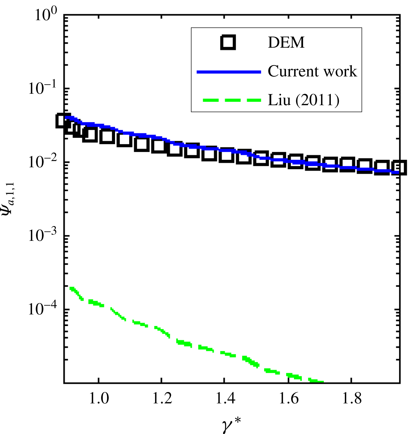
, their determination depended on the availability of individual (not continuum) collision quantities, namely the distribution of impact velocities, which they obtained from DEM simulations of simple shear flow. In other words, their approach is incompatible with a strictly continuum theory, since individual collision quantities (impact velocities) are unavailable. A method to overcome this shortcoming was recently proposed by Liu (Reference Liu2011), who provided an analytical prediction of the total impact velocity distribution (including normal and tangential components of velocity) as a function of the (continuum quantity)
 $T_{s}$
, and determined
 $\unicode[STIX]{x1D713}_{a}$
by integrating the distribution over the total impact velocities where agglomeration occurs. This approach, which was based on an assumption that the total impact velocity governs aggregation, was not validated with simulation or experimental data.
An accurate prediction of the success factors
 $\unicode[STIX]{x1D713}_{a}$
and
 $\unicode[STIX]{x1D713}_{b}$
relies on an accurate estimation of the distribution of impact velocities, and consequently their continuum counterpart,
 $T_{s}$
. A crucial term in the granular energy balance is the sink due to inelastic (dissipative) collisions. The amount of dissipation is quantified by the coefficient of restitution
 $e$
, which is the ratio of the magnitude of the post-collisional normal (head-on) impact velocity of a particle pair to its pre-collisional counterpart. For collisions between cohesive particles, the particles will accelerate towards each other due to the attractive force, undergo a collision at a higher impact velocity than non-cohesive particles, and therefore dissipate more energy (Seville et al.
Reference Seville, Willett and Knight2000). This additional dissipation due to cohesion needs to be taken into account in the granular energy balance. Arastoopour & Kim (Reference Arastoopour and Kim2002) accounted for the extra dissipation that occurs during aggregation in their derivation of a kinetic-theory-based continuum theory that accounts for cohesive aggregation only (no breakage). Even for collisions that do not result in aggregation, however, additional energy is also dissipated during collisions between cohesive particles, as demonstrated by numerous previous experiments, theory and simulations (e.g. Davis, Serayssol & Hinch Reference Davis, Serayssol and Hinch1986; Thornton & Ning Reference Thornton and Ning1998; Weber, Hoffman & Hrenya Reference Weber, Hoffman and Hrenya2004; Donahue et al.
Reference Donahue, Davis, Kantak and Hrenya2012; Gollwitzer et al.
Reference Gollwitzer, Rehberg, Kruelle and Huang2012; Murphy & Subramaniam Reference Murphy and Subramaniam2017). Another approach for incorporating cohesion into the kinetic theory that accounts for the additional dissipation – whether or not aggregation or breakage occurs – is via the use of an ‘effective’ coefficient of restitution
 $e_{eff}$
, which is smaller than the intrinsic coefficient of restitution
 $e_{int}$
for the material under consideration. Murphy & Subramaniam (Reference Murphy and Subramaniam2015) used a fundamentally based
 $e_{eff}$
to solve the granular energy balance in the homogeneous cooling system (HCS). Their continuum theory, however, is restricted to dilute flows undergoing homogeneous cooling.
The first overarching goal of this work, as described in § 2, is to develop a general continuum framework for the rapid flow of solid particles that experience short-range cohesive forces. The specific objectives are twofold: (i) to develop fundamentally based aggregation and breakage kernels including success factors of aggregation
 $\unicode[STIX]{x1D713}_{a}$
and breakage
 $\unicode[STIX]{x1D713}_{b}$
based on the granular temperature
 $T_{s}$
and (ii) to accurately predict
 $T_{s}$
for cohesive particles using the granular energy balance. To achieve the first aim, the distribution of normal impact velocities is fundamentally determined as a function of
 $T_{s}$
, as we show that the normal component of the impact velocity (rather than the total, as previously assumed (Liu Reference Liu2011)) solely determines whether agglomeration or rebound occurs during a collision. Then,
 $\unicode[STIX]{x1D713}_{a}$
and
 $\unicode[STIX]{x1D713}_{b}$
are determined by integrating over the impact velocities at which aggregation and breakage occur. In order to achieve the second aim of accurately predicting
 $T_{s}$
, a mean effective coefficient of restitution
 $\langle e_{eff}\rangle$
is determined based on the distribution of impact velocities and then recast in terms of the continuum quantity
 $T_{s}$
. The resulting
 $\langle e_{eff}\rangle$
is then substituted into all of the kinetic-theory-based transport coefficients. Discrete element method simulations of simple shear flow (SSF) are then utilized for verification of the impact velocity distribution developed for the new continuum theory presented here. For the purposes of simplicity, we focus on cohesive granular materials (no gas phase), although the continuum theory can be extended to gas–solid flows in a straightforward manner. In § 2, we develop continuum equations that are general, i.e. they are cast in a manner that does not depend on the specific type of short-range cohesion under consideration. As expected, however, some of the closures contain quantities that are cohesion-specific (e.g. critical velocity of agglomeration) and thus need to be evaluated for the equations to be applied to a specific type of cohesion.
Generally speaking, these cohesion-specific quantities appearing in the population balance (critical velocities
 $v_{a,V,V^{\prime },crit}$
and
 $v_{b,V,V^{\prime },crit}$
, collision diameter
 $d_{V,V^{\prime }}$
and daughter distribution
 $b(V\mid T_{s},V^{\prime },V^{\prime \prime })$
) and kinetic theory (effective coefficient of restitution
 $e_{eff}$
) can be found via experiments or particle–particle cohesion models (e.g. Hamaker model for van der Waals forces (Hamaker Reference Hamaker1937)). In several previous works involving liquid bridges, each of these cohesion-specific quantities was determined from pendulum experiments (e.g. Davis, Rager & Good Reference Davis, Rager and Good2002; Donahue et al.
Reference Donahue, Hrenya, Davis, Nakagawa, Zelinskaya and Joseph2010, Reference Donahue, Davis, Kantak and Hrenya2012). For fine particles in which van der Waals forces play an important role (
 ${\lesssim}100~\unicode[STIX]{x03BC}\text{m}$
diameter for flows in ambient air), however, experimental apparatuses like pendulums (e.g. Donahue et al.
Reference Donahue, Hrenya, Davis, Nakagawa, Zelinskaya and Joseph2010, Reference Donahue, Davis, Kantak and Hrenya2012) are infeasible due to the small size of the particles. For some forms of cohesion, such challenges can be overcome if the system can be scaled up through non-dimensionalization (i.e. colliding larger particles, which are easier to control and observe, as was done for pendulum experiments involving larger particles) (Donahue et al.
Reference Donahue, Hrenya, Davis, Nakagawa, Zelinskaya and Joseph2010, Reference Donahue, Davis, Kantak and Hrenya2012). However, a more challenging obstacle is the extension of such experiments to collisions between large agglomerates, in which the control of agglomerate shape and orientation just prior to collision is non-trivial at best. Alternatively, the cohesion-specific quantities (
 $v_{a,V,V^{\prime },crit}$
,
 $v_{b,V,V^{\prime },crit}$
,
 $d_{V,V^{\prime }}$
,
 $b(V\mid T_{s},V^{\prime },V^{\prime \prime })$
and
 $e_{eff}$
) can be found using force models for particle–particle cohesion (and contact). Although the determination of an accurate cohesion model is challenging due to the extreme sensitivity of the cohesive force to the separation distance and hence particle roughness (Rabinovich et al.
Reference Rabinovich, Adler, Ata, Singh and Moudgil2000; Liu et al.
Reference Liu, LaMarche, Kellogg, Leadley and Hrenya2016a
), such models can be applied in a straightforward manner to collisions involving complex multi-particle agglomerates. More specifically, analytical solutions of cohesion models (Seville et al.
Reference Seville, Willett and Knight2000) for cohesion-specific quantities like
 $e_{eff}$
have been found for van der Waals forces and capillary forces (e.g. Bryan & Rober Pfeffer Reference Bryan and Rober Pfeffer1991; Weber et al.
Reference Weber, Hoffman and Hrenya2004), although such analytical solutions are generally tractable only for collisions between single particles. Another approach is to numerically determine the cohesion-specific quantities from controlled two-particle or multi-particle DEM simulations that incorporate the cohesion model, as has been done in many works (e.g. Kafui & Thornton Reference Kafui and Thornton2000; Ringl et al.
Reference Ringl, Bringa, Bertoldi and Urbassek2012). Unlike experiments, the simulation of complex collision orientations with larger agglomerates of various shapes is straightforward. Nonetheless, a challenge of such controlled simulations is that the most frequent types of collision orientations are not known a priori for a given flow system. Another option, which has not been explored yet, is the determination of the cohesion-specific quantities,
 $v_{a,V,V^{\prime },crit}$
,
 $v_{b,V,V^{\prime },crit}$
,
 $d_{V,V^{\prime }}$
,
 $b(V\mid T_{s},V^{\prime },V^{\prime \prime })$
and
 $e_{eff}$
, from relatively simple DEM simulations of many-particle flows (e.g. simple shear flow). This approach has the advantage of sampling the collision orientations from a simplified flow expected to have similar orientation characteristics to the ultimate flow of interest (e.g. shear-driven system). This approach, alongside simulations of controlled two-particle collisions, will be explored in this work.
Accordingly, the second overarching goal of this work is to determine the cohesion-specific quantities needed for the new theory to be fully specified and to be applied to practical situations, as described in §§ 3 and 4. Specific objectives of this second portion of the work are to (iii) demonstrate the determination of the cohesion-specific quantities (
 $v_{a,V,V^{\prime },crit}$
,
 $v_{b,V,V^{\prime },crit}$
,
 $d_{V,V^{\prime }}$
,
 $b(V\mid T_{s},V^{\prime },V^{\prime \prime })$
and
 $e_{eff}$
) needed for the closure of the new continuum theory derived in § 2 via consideration of a specific source of cohesion and (iv) provide initial validation for the resulting fully specified continuum theory. For simplicity, the focus here will be on granular systems (no fluid phase); extension of kinetic-theory balances to multiphase flows is well documented elsewhere (e.g. Gidaspow Reference Gidaspow1994; Jackson Reference Jackson2000; Pannala et al.
Reference Pannala, Syamlal and O’Brien2011). Moreover, we consider van der Waals cohesion, although the methods demonstrated here to obtain the cohesion-specific quantities can be applied to other mechanisms of cohesion. Finally, we restrict ourselves to lightly cohesive systems with only single particles and two-particle agglomerates (singlets and doublets respectively). This simplification essentially isolates any sources of error in the predictions to those stemming from the new closures derived here. With regards to the approach for objective (iii), controlled two-particle DEM simulations are used to determine the critical velocity of aggregation
 $v_{a,V,V^{\prime },crit}$
and the effective coefficient of restitution
 $e_{eff}$
, and SSF simulations are used to determine the critical velocity of breakage
 $v_{b,V,V^{\prime },crit}$
and the collision cylinder diameter
 $d_{V,V^{\prime }}$
. The population-balance closures are then verified (coding accuracy) using SSF and validated (theory accuracy) using the HCS. Further, the appropriateness of using
 $\langle e_{eff}\rangle$
in kinetic-theory expressions is demonstrated in both the SSF and the HCS.
2 Theory development
2.1 Population balance
In the population balance, each agglomerate size is treated as its own species, with a separate balance equation on the number density of that species. In its most general form, the population balance is given by (Ramkrishna Reference Ramkrishna2000)
 $$\begin{eqnarray}\frac{\unicode[STIX]{x2202}}{\unicode[STIX]{x2202}t}[n(V,t)]+\unicode[STIX]{x1D735}\boldsymbol{\cdot }[\boldsymbol{u}(V,t)n(V,t)]=S(V,t)\end{eqnarray}$$
for an agglomerate of volume
 $V$
with a number density of
 $n$
and velocity
 $\boldsymbol{u}$
. The left-hand side represents the transient and convective contributions, while the right-hand side represents the source and/or sinks of agglomerates of volume
 $V$
. More specifically, the net generation,
 $S$
, is defined as (Ramkrishna Reference Ramkrishna2000)
 $$\begin{eqnarray}S(V,t)=B_{a}(V,t)-D_{a}(V,t)+B_{b}(V,t)-D_{b}(V,t),\end{eqnarray}$$
where
 $B_{a}$
is the volumetric birth rate due to aggregation,
 $D_{a}$
is the death rate due to aggregation,
 $B_{b}$
is the birth rate due to breakage and
 $D_{b}$
is the death rate due to breakage. It should be noted that birth and death due to nucleation (coalescence due to a phase change or chemical reaction) are not considered here, as the focus of this work is on the aggregation and breakage kernels.
The birth rate due to aggregation used here is similar to that generally given in the literature (Ramkrishna Reference Ramkrishna2000), and is defined as
 $$\begin{eqnarray}B_{a}(V,t)=\frac{1}{2}\int _{0}^{V}(1+\unicode[STIX]{x1D6FF}_{V-V^{\prime },V^{\prime }})\unicode[STIX]{x1D6FD}(V^{\prime },V-V^{\prime },t)n(V-V^{\prime },t)n(V^{\prime },t)\,\text{d}V,\end{eqnarray}$$
where
 $\unicode[STIX]{x1D6FD}(V^{\prime },V-V^{\prime },t)$
is the ‘aggregation kernel’, which represents the frequency of aggregation events (i.e. when two agglomerates collide and form a larger agglomerate) between agglomerates of sizes
 $V^{\prime }$
and
 $V-V^{\prime }$
, per unit volume and per number density of each agglomerate size undergoing aggregation. Here,
 $\unicode[STIX]{x1D6FF}_{V-V^{\prime },V^{\prime }}$
is the Kronecker delta function,
 $$\begin{eqnarray}\unicode[STIX]{x1D6FF}_{V-V^{\prime },V^{\prime }}=\left\{\begin{array}{@{}ll@{}}0, & V-V^{\prime }\neq V^{\prime },\\ 1, & V-V^{\prime }=V^{\prime }.\end{array}\right.\end{eqnarray}$$
It is worthwhile to note that
 $1+\unicode[STIX]{x1D6FF}_{V-V^{\prime },V}$
ensures the proper counting of birth due to aggregation events during symmetric aggregation (i.e. the case of
 $V^{\prime }=V-V^{\prime }$
is only summed over by the integrand in (2.3) once, whereas all other combinations
 $V^{\prime }\neq V-V^{\prime }$
are summed over twice), and does not appear in prior works. It should also be noted that the birth rate due to aggregation given in (2.3) only accounts for aggregation events in which all of the particles in the agglomerates of sizes
 $V^{\prime }$
and
 $V-V^{\prime }$
form an agglomerate of size
 $V$
; collisions involving simultaneous aggregation and breakage in which an agglomerate of size
 $V$
is formed are accounted for in the birth rate due to breakage (
 $B_{b}$
), as detailed below.
Similarly, the rate of death rate due to aggregation is taken as
 $$\begin{eqnarray}D_{a}(V,t)=\int _{0}^{\infty }(1+\unicode[STIX]{x1D6FF}_{V,V^{\prime }})\unicode[STIX]{x1D6FD}(V,V^{\prime },t)n(V,t),n(V^{\prime },t)\,\text{d}V^{\prime },\end{eqnarray}$$
where
 $\unicode[STIX]{x1D6FF}_{V,V^{\prime }}$
is the corresponding Kronecker delta function. Again, the
 $1+\unicode[STIX]{x1D6FF}_{V,V^{\prime }}$
term is not included in prior works. This term is included here to represent the events in which two agglomerates of size
 $V$
collide and aggregate, thereby leading to the death of two agglomerates of size
 $V$
.
Before presenting the equations for the birth and death rates due to breakage (
 $B_{b}$
and
 $D_{b}$
), it is worth noting that an agglomerate can break due to (i) collision with another agglomerate, (ii) collision with a wall, (iii) shear forces from a surrounding fluid or (iv) centrifugal forces arising from its own rotation (Ramachandran et al.
Reference Ramachandran, Immanuel, Stepanek, Litster and Doyle2009; Donahue et al.
Reference Donahue, Davis, Kantak and Hrenya2012). Mechanism (i) is the focus of this work, although the approach taken here could easily be extended to mechanism (ii). Consequently, the birth and death rates due to breakage will take a form that is proportional to the frequency of collisions between two agglomerates, and hence the concentration of each (similar to the birth and death rates due to aggregation,
 $B_{a}$
and
 $D_{a}$
).
The birth rate due to breakage is defined similarly to previous works (Fan et al. Reference Fan, Marchisio and Fox2004) as
 $$\begin{eqnarray}B_{b}(V,t)=\int _{0}^{\infty }\int _{0}^{\infty }\left(\frac{1+\unicode[STIX]{x1D6FF}_{V^{\prime },V^{\prime \prime }}}{2}\right)\unicode[STIX]{x1D6FC}(V^{\prime },V^{\prime \prime })b(V\mid T_{s},V^{\prime },V^{\prime \prime })n(V^{\prime },t)n(V^{\prime \prime },t)\,\text{d}V^{\prime }\,\text{d}V^{\prime \prime },\end{eqnarray}$$
where
 $\unicode[STIX]{x1D6FC}(V^{\prime },V)$
is the breakage kernel representing the frequency of breakage events between agglomerates of sizes
 $V^{\prime }$
and
 $V^{\prime \prime }$
. The quantity
 $b(V\mid T_{s},V^{\prime },V^{\prime \prime })$
is the daughter distribution function, which gives the number of agglomerates of size
 $V$
produced by a collision resulting in any breakage of agglomerates of size
 $V^{\prime }$
and
 $V^{\prime \prime }$
for a system of mixture granular temperature
 $T_{s}$
(i.e. a measure of the fluctuating kinetic energy of particles and agglomerates). The term
 $(1+\unicode[STIX]{x1D6FF}_{V^{\prime },V^{\prime \prime }})/2$
is included to prevent double counting of breakage events due to the second integral.
Finally, the death rate due to breakage (Fan et al. Reference Fan, Marchisio and Fox2004) is given by
 $$\begin{eqnarray}D_{b}(V,t)=\int _{0}^{\infty }\unicode[STIX]{x1D6FC}(V,V^{\prime })n(V,t)n(V^{\prime },t)\,\text{d}V^{\prime }.\end{eqnarray}$$
In this work, the aggregation kernel
 $\unicode[STIX]{x1D6FD}$
used in (2.3) and (2.5) and the breakage kernel
 $\unicode[STIX]{x1D6FC}$
used in (2.6) and (2.7) are defined in a similar manner to previous literature (Goldschmidt Reference Goldschmidt2001). A notable exception is that the breakage kernel
 $\unicode[STIX]{x1D6FC}$
is now also dependent on the frequency of collisions (Fan et al.
Reference Fan, Marchisio and Fox2004),
 $$\begin{eqnarray}\displaystyle & \displaystyle \unicode[STIX]{x1D6FD}(V,V^{\prime })=\unicode[STIX]{x1D713}_{a}(V,V^{\prime })\frac{\unicode[STIX]{x1D714}(V,V^{\prime })}{n(V)n(V^{\prime })}, & \displaystyle\end{eqnarray}$$
 $$\begin{eqnarray}\displaystyle & \displaystyle \unicode[STIX]{x1D6FC}(V,V^{\prime })=\unicode[STIX]{x1D713}_{b}(V,V^{\prime })\frac{\unicode[STIX]{x1D714}(V,V^{\prime })}{n(V)n(V^{\prime })}, & \displaystyle\end{eqnarray}$$
where
 $\unicode[STIX]{x1D713}_{a}(V,V^{\prime })$
and
 $\unicode[STIX]{x1D713}_{b}(V,V^{\prime })$
are the ‘success factors’ of aggregation and breakage respectively, which represent the fraction of collisions that result in agglomeration or breakage. Here,
 $\unicode[STIX]{x1D714}(V,V^{\prime })$
is the collision frequency per unit volume of agglomerates of size
 $V$
and
 $V^{\prime }$
, given by
 $$\begin{eqnarray}n(V)n(V^{\prime })\unicode[STIX]{x03C0}d_{V,V^{\prime }}^{3}g_{0}\left[\frac{4}{d_{V,V^{\prime }}}\left(\frac{T_{s}}{\unicode[STIX]{x03C0}}\frac{m_{V}\,\text{dof}_{V^{\prime }}+m_{V^{\prime }}\,\text{dof}_{V}}{m_{V}m_{V^{\prime }}}\right)^{1/2}-\frac{2}{3}(\unicode[STIX]{x1D735}\boldsymbol{\cdot }\boldsymbol{u}_{\boldsymbol{s}})\right],\end{eqnarray}$$
 $T_{s}$
is the granular temperature (which represents the variance of the velocities of individual particles relative to the local motion),
 $m_{V}$
is the mass of an agglomerate of size
 $V$
,
 $g_{0}$
is the radial distribution function (e.g. that given by Carnahan Starling (Mansoori Reference Mansoori1971)) and
 $d_{V,V^{\prime }}$
is the collision cylinder diameter of agglomerates of sizes
 $V$
and
 $V^{\prime }$
. A collision cylinder diameter interpretation is adopted here as agglomerates are aspherical, and thus whether or not they are in contact (undergoing a collision) is no longer a function of just position, but also orientation. The term
 $\text{dof}_{V}$
represents the sum of translational and rotational degrees of freedom of an agglomerate of size
 $V$
(e.g. for frictionless particles, a singlet has three translational degrees of freedom and
 $\text{dof}_{1}=3$
, a doublet has three translational and two rotational degrees of freedom and
 $\text{dof}_{2}=5$
). It should be noted that this expression for the collision frequency does not take into account interphase slip, and does not assume the system to be homogeneous. In the validation systems explored here, there is no interphase slip and the system is homogeneous, so this expression is applicable.
To recap, the population-balance equations for each agglomerate size (2.1) include sink and source terms for the rates of birth and death due to aggregation and breakage (2.3), (2.5)–(2.7). The fundamental closures for the sink and source terms depend on the aggregation and breakage kernels,
 $\unicode[STIX]{x1D6FD}$
and
 $\unicode[STIX]{x1D6FC}$
respectively, i.e. the frequency of aggregation and breakage events (2.8)–(2.9). The kernels now require a closure for the success factors of aggregation and breakage (
 $\unicode[STIX]{x1D713}_{a}$
and
 $\unicode[STIX]{x1D713}_{b}$
).
2.2 Population-balance closures: success factors of aggregation
 $(\unicode[STIX]{x1D713}_{a})$
and breakage
$(\unicode[STIX]{x1D713}_{b})$


As mentioned above, the closures for the aggregation
 $(\unicode[STIX]{x1D6FD}(V,V^{\prime }))$
and breakage
 $(\unicode[STIX]{x1D6FC}(V,V^{\prime }))$
kernels are proportional to the fraction of collisions that result in aggregation or breakage, or the success factors
 $\unicode[STIX]{x1D713}_{a}$
and
 $\unicode[STIX]{x1D713}_{b}$
. Numerous previous works (e.g. Lian, Thornton & Adams Reference Lian, Thornton and Adams1998; Jackson Reference Jackson2000; Calvert et al.
Reference Calvert, Ghadiri and Tweedie2009; Donahue et al.
Reference Donahue, Hrenya, Davis, Nakagawa, Zelinskaya and Joseph2010, Reference Donahue, Davis, Kantak and Hrenya2012; Ringl et al.
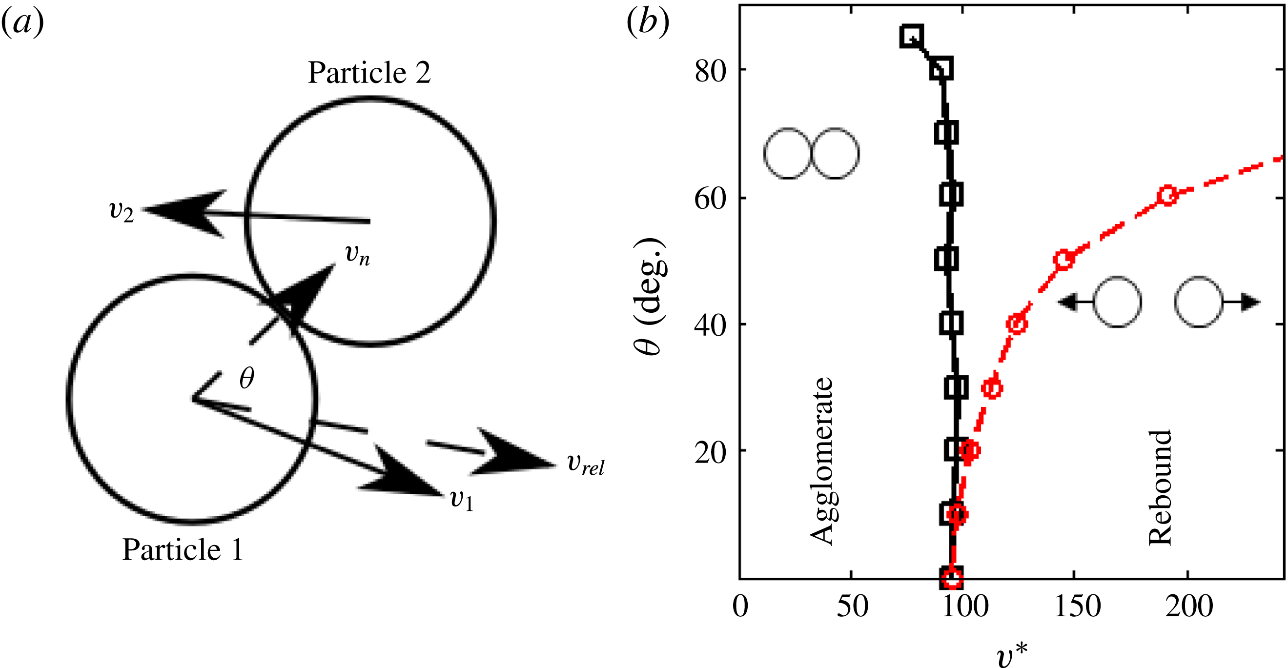
Reference Ringl, Bringa, Bertoldi and Urbassek2012) have demonstrated that the result of a collision between two cohesive bodies (single particles and/or agglomerates) depends on their impact (relative) velocity. Moreover, a series of numerical simulations of two-particle collisions of cohesive particles indicates that there is a normal component of the impact velocity,
 $v_{n}$
, which demarcates the agglomeration and breakage outcomes, as illustrated in figure 1 (black solid line), which is consistent with past experimental observations for cohesion due to liquid (Donahue et al.
Reference Donahue, Hrenya, Davis, Nakagawa, Zelinskaya and Joseph2010, Reference Donahue, Davis, Kantak and Hrenya2012). Accordingly,
 $\unicode[STIX]{x1D713}_{a}$
and
 $\unicode[STIX]{x1D713}_{b}$
should depend on the distribution of
 $v_{n}$
in a given system. In terms of continuum variables, the distribution of individual collision impact velocities is related to the (continuum) granular temperature, since the latter is a measure of the particle velocity distribution relative to the local mean velocity (i.e. a measure of particle velocity fluctuations). Therefore, the closures for the success factors
 $\unicode[STIX]{x1D713}_{a}$
and
 $\unicode[STIX]{x1D713}_{b}$
should depend on
 $T_{s}$
.
(a) Collision schematic;
 $\boldsymbol{v}_{rel}=\boldsymbol{v}_{1}-v_{2}$
. (b) Regime map of binary collisions between two cohesive primary particles (singlets). Here,
 $v^{\ast }$
is a non-dimensionalized impact velocity (
 $=v/(A/(\unicode[STIX]{x1D70C}d_{1}^{3}))^{1/2}$
, where
 $A$
is the Hamaker constant). The black line and points show the magnitude of the normal component of the critical impact velocity
 $(v_{a,1,1,crit}^{\ast })$
, which demarcates aggregation and rebound from DEM simulations of cohesive particles described in § 3.2.1. The red dashed line and points show the magnitude of the critical total relative impact velocity
 $(v_{a,tot,1,1,crit}^{\ast })$
. It should be noted that the normal component
 $v_{a,1,1,crit}^{\ast }$
is approximately independent of the impact angle, whereas the total component
 $v_{a,tot,1,1,crit}^{\ast }$
is not.

Expressions similar to previous works (Kantak et al. Reference Kantak, Hrenya and Davis2009; Liu Reference Liu2011) are used to calculate the success factors of both agglomeration and breakage. Namely, the success factors are defined here as
 $$\begin{eqnarray}\displaystyle & \displaystyle \unicode[STIX]{x1D713}_{a}(V,V^{\prime })=\int _{0}^{v_{a,V,V^{\prime },crit}}f(v_{n})\,\text{d}v_{n}, & \displaystyle\end{eqnarray}$$
 $$\begin{eqnarray}\displaystyle & \displaystyle \unicode[STIX]{x1D713}_{b}(V,V^{\prime })=\int _{v_{b,V,V^{\prime },crit}}^{\infty }f(v_{n})\,\text{d}v_{n}, & \displaystyle\end{eqnarray}$$
where
 $v_{a,V,V^{\prime },crit}$
and
 $v_{b,V,V^{\prime },crit}$
are the critical normal impact velocities of agglomeration and breakage for collisions between agglomerates of sizes
 $V$
and
 $V^{\prime }$
respectively. For the purposes of generality, the critical velocities of agglomeration and breakage are allowed to take on different values for a given pair of colliding objects (i.e. the critical velocities of agglomeration and breakage are different from each other), as well as for different sizes of agglomerates undergoing collisions. Here,
 $f(v_{n})$
is the normalized probability density function that a collision between agglomerates will have a normal impact velocity of
 $v_{n}$
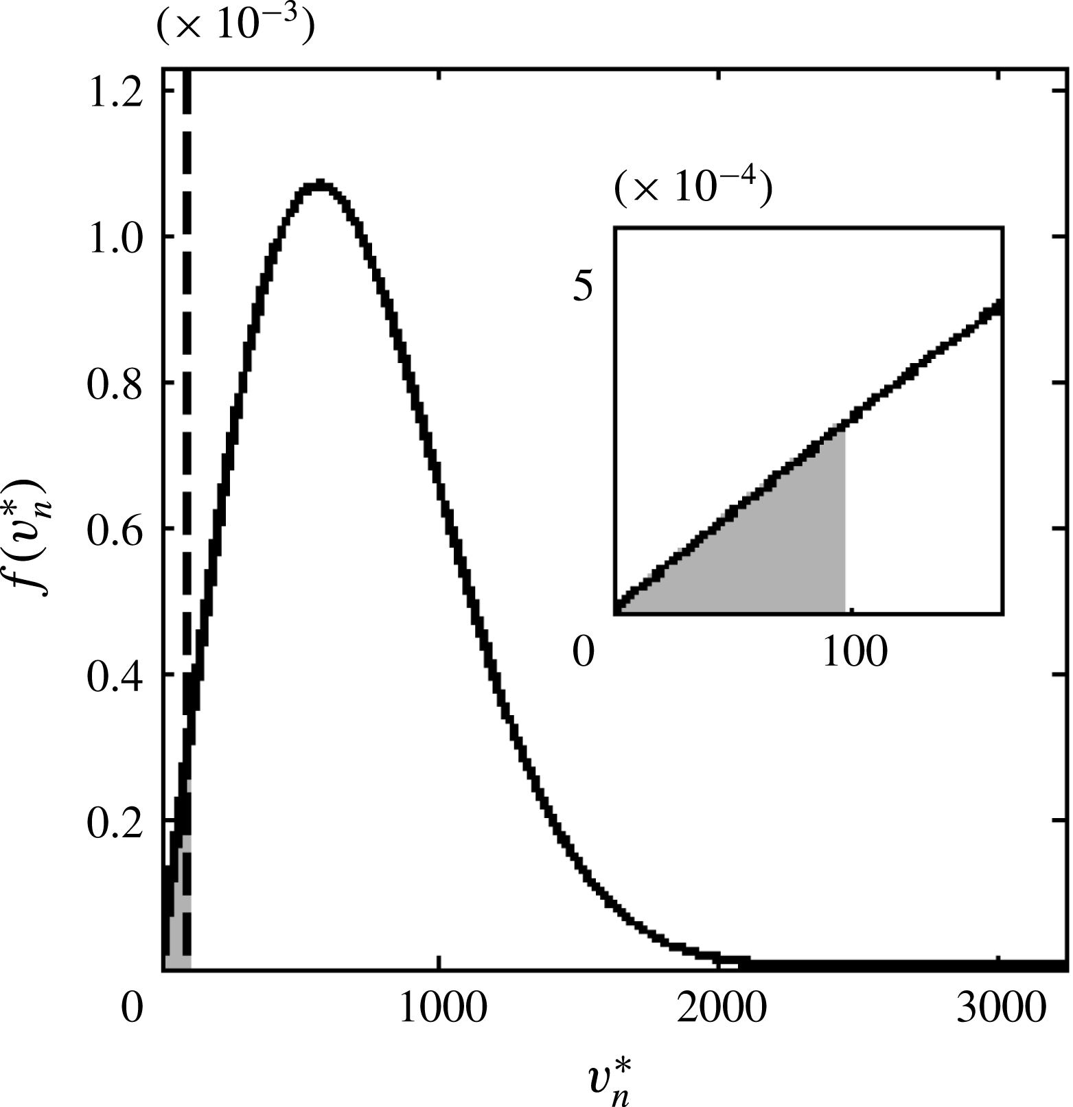
. This method for calculating the success factors is depicted graphically in figure 2 for
 $\unicode[STIX]{x1D713}_{a}$
. For a given system, the critical velocities of agglomeration (vertical dashed line in figure 2) and breakage depend on the type of cohesion (van der Waals, liquid bridging, etc.) and materials involved, and can be determined mathematically from a particle–particle cohesion model (i.e. analytical solutions to two-body collisions or the DEM (e.g. Bryan & Rober Pfeffer Reference Bryan and Rober Pfeffer1991; Weber et al.
Reference Weber, Hoffman and Hrenya2004)) or from experiments (e.g. Donahue et al.
Reference Donahue, Davis, Kantak and Hrenya2012). Accordingly, general expressions for the success factors as functions of these critical velocities can be determined if
 $f(v_{n})$
is known. Kantak et al. (Reference Kantak, Hrenya and Davis2009) determined
 $f(v_{n})$
from a Gaussian fit of DEM data, which confirmed the accuracy of the expressions above but is not useful in a general continuum framework since the impact velocities are quantities specific to an individual collision (i.e. not continuum quantities) and thus remain unknown. Instead, we derive an analytical prediction of
 $f(v_{n})$
as a function of the granular temperature, a flow variable that is solved for within the continuum framework. Liu (Reference Liu2011) analytically determined the distribution of total relative velocity
 $(v_{tot})$
as a function of the granular temperature
 $T_{s}$
. However, figure 1 demonstrates that it is more appropriate to consider only the normal component of the impact velocity, for which the critical value is constant across various impact angles (
 $\unicode[STIX]{x1D703}$
). Put another way, considering
 $\unicode[STIX]{x1D713}$
as a function of
 $v_{n}$
only, instead of
 $\unicode[STIX]{x1D713}$
as a function of
 $v_{tot}$
and
 $\unicode[STIX]{x1D703}$
, is much cleaner since the
 $\unicode[STIX]{x1D703}$
distribution (also comprising quantities specific to individual collisions and not solved for in the continuum framework) does not have to be assumed or estimated. In the following, a novel analytical closure for
 $f(v_{n})$
is derived as a function of
 $T_{s}$
.
Illustrative schematic of prediction of the success factor of aggregation for particles. The solid black line shows the normal impact velocity distribution
 $f(v_{n})$
. The dashed black line shows the critical velocity of aggregation
 $v_{a,V,V^{\prime },crit}$
. The grey area, which is shown expanded in the inset, is the success factor of aggregation
 $\unicode[STIX]{x1D713}_{a}$
.

Assuming a Maxwellian distribution of particle velocities and independence of each velocity component for agglomerates of size
 $V$
, the magnitude of the velocity distribution of the agglomerate (or single particle) is given by
 $$\begin{eqnarray}p(\boldsymbol{v})=p(v_{x})p(v_{y})p(v_{z})=\frac{1}{\sqrt{2\unicode[STIX]{x03C0}\unicode[STIX]{x1D70E}_{\boldsymbol{u}}^{2}}}\exp \left[-\frac{(\boldsymbol{v}-\boldsymbol{u})^{2}}{2\unicode[STIX]{x1D70E}_{\boldsymbol{u}}^{2}}\right],\end{eqnarray}$$
where
 $\boldsymbol{v}$
is the agglomerate translational velocity,
 $\boldsymbol{u}$
is the local mean velocity of the agglomerates of the same size and
 $v_{x},v_{y},v_{z}$
are the
 $x$
,
 $y$
and
 $z$
components of the agglomerate translational velocity respectively. The term
 $\unicode[STIX]{x1D70E}_{\boldsymbol{u}}^{2}$
is the variance of the magnitude of velocities of agglomerates of the same size. It is related to the granular energy
 $E$
and granular temperature by
 $$\begin{eqnarray}E=3T_{s,V}/2=\text{dof}_{V}m_{V}\unicode[STIX]{x1D70E}_{\boldsymbol{u}}^{2}/6.\end{eqnarray}$$
The assumption of isotropy gives
 $$\begin{eqnarray}p(v_{x})=p(v_{y})=p(v_{z}).\end{eqnarray}$$
It should be noted that the incorporation of anisotropy is highly non-trivial (Sela & Goldhirsch Reference Sela and Goldhirsch1998), and it may not be necessary to incorporate it in the theory even when such higher-order effects are present (Mitrano et al. Reference Mitrano, Zenk, Benyahia, Galvin, Dahl and Hrenya2013; Fullmer & Hrenya Reference Fullmer and Hrenya2017). Further, the SSF and HCS explored in the current work are isotropic. Application of (2.15) to (2.13) yields
 $$\begin{eqnarray}p(\boldsymbol{v})=p(v_{x})^{3}=\frac{1}{\sqrt{2\unicode[STIX]{x03C0}\unicode[STIX]{x1D70E}_{\boldsymbol{u}}^{2}}}\exp \left[-\frac{3(v_{x}-u_{x})^{2}}{2\unicode[STIX]{x1D70E}_{\boldsymbol{u}}^{2}}\right],\end{eqnarray}$$
where
 $u_{x}$
is the mean velocity of the agglomerate size in the
 $x$
direction. By solving (2.14) for
 $\unicode[STIX]{x1D70E}_{\boldsymbol{u}}^{2}$
, and substituting
 $\unicode[STIX]{x1D70E}_{\boldsymbol{u}}^{2}$
and (2.16) into (2.13), the velocity distribution for a single agglomerate (or particle) in one direction becomes
 $$\begin{eqnarray}p(v_{x})=\frac{1}{\sqrt{6\unicode[STIX]{x03C0}T_{s,V}/(m_{V}\,\text{dof}_{V})}}\exp \left[-\frac{(v_{x}-u_{x})^{2}}{6T_{s,V}/(m_{V}\,\text{dof}_{V})}\right],\end{eqnarray}$$
where
 $p$
is the normalized probability distribution function,
 $v_{x}$
is the
 $x$
component of the velocity of an individual agglomerate and
 $u_{x}$
is the
 $x$
component of the local mean species velocity. Assuming that particles and/or agglomerates of different masses display an approximate equipartition of energy (
 $T_{s,V}=T_{s,V^{\prime }}\equiv T_{s}$
), (2.17) can be rewritten for two agglomerates of different masses
 $V$
and
 $V^{\prime }$
as
 $$\begin{eqnarray}\displaystyle & \displaystyle p(v_{x,V})=\frac{1}{\sqrt{6\unicode[STIX]{x03C0}T_{s}/(m_{V}\,\text{dof}_{V})}}\exp \left[\frac{-(v_{x,V}-u_{x,V})^{2}}{6T_{s}/(m_{V}\,\text{dof}_{V})}\right], & \displaystyle\end{eqnarray}$$
 $$\begin{eqnarray}\displaystyle & \displaystyle p(v_{x,V^{\prime }})=\frac{1}{\sqrt{6\unicode[STIX]{x03C0}T_{s}/(m_{V^{\prime }}\,\text{dof}_{V^{\prime }})}}\exp \left[\frac{-(v_{x,V^{\prime }}-u_{x,V^{\prime }})^{2}}{6T_{s}/(m_{V^{\prime }}\,\text{dof}_{V^{\prime }})}\right]. & \displaystyle\end{eqnarray}$$
By manipulating (2.19) (redefining the coordinate system to replace
 $v_{x,V^{\prime }}$
with
 $-v_{x,V^{\prime }}$
and
 $u_{x,V^{\prime }}$
with
 $-u_{x,V^{\prime }}$
throughout), the following is obtained:
 $$\begin{eqnarray}p(-v_{x,V^{\prime }})=\frac{1}{\sqrt{6\unicode[STIX]{x03C0}T_{s}/(m_{V^{\prime }}\,\text{dof}_{V^{\prime }})}}\exp \left[\frac{-(-v_{x,V^{\prime }}+u_{x,V^{\prime }})^{2}}{6T_{s}/(m_{V^{\prime }}\,\text{dof}_{V^{\prime }})}\right].\end{eqnarray}$$
Combining the two Gaussians (2.18) and (2.20), and assuming molecular chaos (velocities of colliding particles are not correlated) gives
 $$\begin{eqnarray}p(v_{x,V}-v_{x,V^{\prime }})=\sqrt{\frac{1}{2\unicode[STIX]{x03C0}T_{s}\displaystyle \left[\frac{3}{m_{V}\,\text{dof}_{V}}+\frac{3}{m_{V^{\prime }}\,\text{dof}_{V^{\prime }}}\right]}}\exp \left[\frac{-(v_{x,V}-v_{x,V^{\prime }}+u_{x,V}-u_{x,V^{\prime }})^{2}}{2T_{s}\displaystyle \left[\frac{3}{m_{V}\,\text{dof}_{V}}+\frac{3}{m_{V^{\prime }}\,\text{dof}_{V^{\prime }}}\right]}\right].\end{eqnarray}$$
It should be noted that this expression includes interphase slip, and assumes that the system is homogeneous. These assumptions are appropriate in the validation systems explored here as there is no interphase slip and these systems are homogeneous. It should also be noted that the direction
 $x$
is arbitrary, so it is defined as the normal direction between the centres of mass of agglomerates of sizes
 $V$
and
 $V^{\prime }$
,
 $$\begin{eqnarray}v_{x,V}-v_{x,V^{\prime }}=v_{n}.\end{eqnarray}$$
In (2.21), the difference in mean velocities in the
 $x$
(normal) direction is the magnitude of the relative velocity between the agglomerate sizes,
 $$\begin{eqnarray}u_{x,V}-u_{x,V^{\prime }}=|\boldsymbol{u}_{\boldsymbol{V}}-\boldsymbol{u}_{\boldsymbol{V}^{\prime }}|,\end{eqnarray}$$
where
 $\boldsymbol{u}_{\boldsymbol{V}}$
and
 $\boldsymbol{u}_{\mathbf{V}^{\prime }}$
are the mean velocities of agglomerates of sizes
 $V$
and
 $V^{\prime }$
. The distribution of normal velocities between agglomerates of sizes
 $V$
and
 $V^{\prime }$
is therefore given by
 $$\begin{eqnarray}p(v_{n})=\sqrt{\frac{1}{2\unicode[STIX]{x03C0}T_{s}\displaystyle \left[\frac{3}{m_{V}\,\text{dof}_{V}}+\frac{3}{m_{V^{\prime }}\,\text{dof}_{V^{\prime }}}\right]}}\exp \left[\frac{-(v_{n}+|\boldsymbol{u}_{\boldsymbol{V}}-\boldsymbol{u}_{\boldsymbol{V}^{\prime }}|)^{2}}{2T_{s}\displaystyle \left[\frac{3}{m_{V}\,\text{dof}_{V}}+\frac{3}{m_{V^{\prime }}\,\text{dof}_{V^{\prime }}}\right]}\right].\end{eqnarray}$$
In order to get the impact velocity distribution
 $f(v_{n})$
, three additional terms (
 $C,H(v_{n})$
and
 $\unicode[STIX]{x1D714}(v_{n})$
) must be multiplied by the distribution of normal velocities,
 $$\begin{eqnarray}f(v_{n})=CH(v_{n})\unicode[STIX]{x1D714}(v_{n})p(v_{n}),\end{eqnarray}$$
where
 $$\begin{eqnarray}H(v_{n})=\left\{\begin{array}{@{}ll@{}}0, & v_{n}<0,\\ 1, & v_{n}\geqslant 0.\end{array}\right.\end{eqnarray}$$
Inclusion of the Heaviside function,
 $H(v_{n})$
, removes the relative velocities of particles moving away from one another (i.e. negative impact velocities) from the distribution as there is no chance of a collision occurring. Here,
 $C$
is a normalization constant which ensures that the distribution is normalized,
 $$\begin{eqnarray}\int _{-\infty }^{\infty }f(v_{n})\,\text{d}v_{n}=1.\end{eqnarray}$$
Therefore,
 $C$
is found by substituting (2.25) into (2.27) and rearranging,
 $$\begin{eqnarray}C=\frac{1}{\displaystyle \int _{-\infty }^{\infty }H(v_{n})\unicode[STIX]{x1D6FA}(v_{n})p(v_{n})\,\text{d}v_{n}}.\end{eqnarray}$$
The term
 $\unicode[STIX]{x1D6FA}(v_{n})$
accounts for the fact that impacts between particles with higher normal velocities will occur more frequently,
 $$\begin{eqnarray}\unicode[STIX]{x1D6FA}(v_{n})=\frac{1}{P(v_{n})},\end{eqnarray}$$
where
 $P(v_{n})$
is the time it takes for two particles destined to collide to approach one another, given by
 $$\begin{eqnarray}P(v_{n})=\frac{l_{arb}}{v_{n}}.\end{eqnarray}$$
Here,
 $l_{arb}$
is the arbitrary distance between the particles when they begin to approach one another. By substituting (2.26), (2.28), (2.29) and (2.30) into (2.25), the distribution of impact velocities becomes
 $$\begin{eqnarray}f(v_{n})=\frac{C_{norm}v_{n}}{2\unicode[STIX]{x03C0}T_{s}\unicode[STIX]{x1D70D}}\exp \left[\frac{-(v_{n}+|\boldsymbol{u}_{\boldsymbol{V}}-\boldsymbol{u}_{\boldsymbol{V}^{\prime }}|)^{2}}{2T_{s}\unicode[STIX]{x1D70D}}\right]H(v_{n}),\end{eqnarray}$$
where
 $$\begin{eqnarray}\unicode[STIX]{x1D70D}=\frac{3}{m_{V}\,\text{dof}_{V}}+\frac{3}{m_{V^{\prime }}\,\text{dof}_{V^{\prime }}}\end{eqnarray}$$
and (2.28) is used to obtain the normalization constant,
 $$\begin{eqnarray}\displaystyle C_{norm}\hspace{-0.1pt}=\hspace{-0.1pt}\frac{C}{l_{arb}}\hspace{-0.1pt}=\hspace{-0.1pt}\frac{T_{s}\unicode[STIX]{x1D70D}}{|\boldsymbol{u}_{\boldsymbol{V}}-\boldsymbol{u}_{\boldsymbol{V}^{\prime }}|\displaystyle \sqrt{\frac{\unicode[STIX]{x03C0}T_{s}\unicode[STIX]{x1D70D}}{2}}\left[1+\sqrt{\unicode[STIX]{x1D70D}}\,\text{erf}\left(\frac{|\boldsymbol{u}_{\boldsymbol{V}}-\boldsymbol{u}_{\boldsymbol{V}^{\prime }}|}{\sqrt{2T_{s}\unicode[STIX]{x1D70D}}}\right)\right]+\unicode[STIX]{x1D70D}\exp \left(\frac{-|\boldsymbol{u}_{\boldsymbol{V}}-\boldsymbol{u}_{\boldsymbol{V}^{\prime }}|^{2}}{2T_{s}\unicode[STIX]{x1D70D}}\right)}.\hspace{-10.00002pt} & & \displaystyle \nonumber\\ \displaystyle & & \displaystyle\end{eqnarray}$$
Further, it should be noted that in the special case where the mean velocities of the two particle types in question are the same (i.e.
 $|\boldsymbol{u}_{\boldsymbol{V}}-\boldsymbol{u}_{\boldsymbol{V}^{\prime }}|=0$
, and also the case when
 $V^{\prime }=V$
), then
 $C_{norm}=1$
and
 $f(v_{n})=(v_{n}/T_{s}\unicode[STIX]{x1D70D})\exp [-v_{n}^{2}/2T_{s}\unicode[STIX]{x1D70D}]H(v_{n})$
.
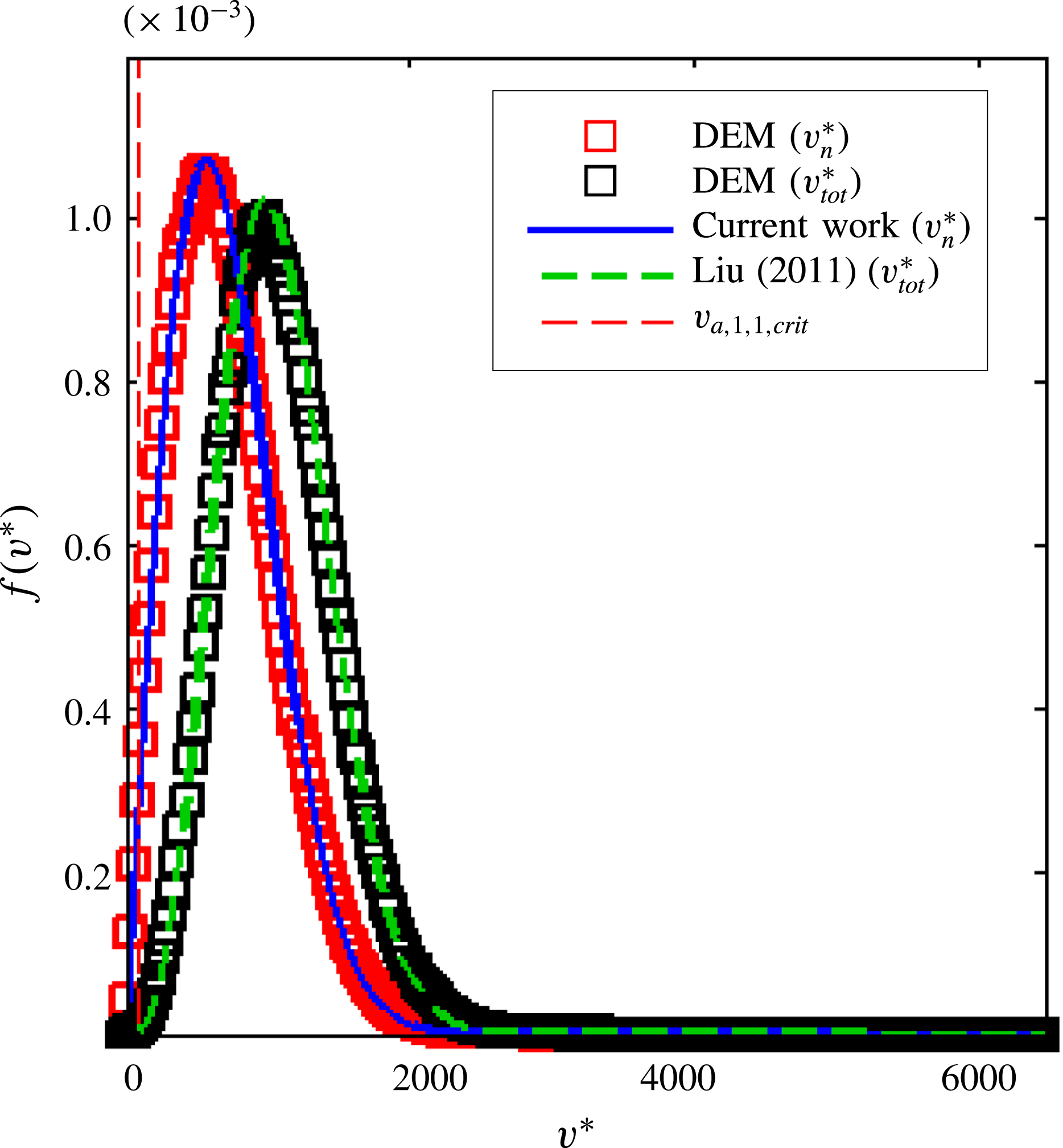
The derivation of
 $f(v_{n})$
presented above is validated in figure 3 via DEM simulations of an SSF system (see § 3.2.2 for details on the method), in which the granular temperature is constant and the local mean velocities of each agglomerate size are equal. The impact velocities were measured just prior to collision in the DEM. Moreover, to isolate any error associated with the new derivation, the
 $T_{s}$
measured in the DEM was used as an input to the predictions for the impact velocity distribution (instead of solving for
 $T_{s}$
using continuum theory) for both the current work (2.34) and the previous prediction for the total impact velocity given by Liu (Reference Liu2011). The results indicate that the prediction of
 $f(v_{n})$
from the current work adequately captures the normal component of the impact velocity distribution observed in the DEM simulations. It is also worth noting that the prediction for the total component of the impact velocity distribution derived by Liu (Reference Liu2011) also matches well with the corresponding DEM data. However, as demonstrated below in figure 9 and alluded to above, the use of the total component of the impact velocity results in an inaccurate prediction of the success factor due to the dependence of its critical velocity on the impact angle, whereas the normal component of the critical velocity is independent of the impact angle (figure 1).
Comparison of normal impact velocity distributions
 $f(v_{n})$
predicted by continuum theory (2.13) and the DEM for singlet–singlet collisions (see § 3.2.2 for more details) in SSF (solid volume fraction
 $\unicode[STIX]{x1D700}_{s}=0.1$
, shear rate
 $\unicode[STIX]{x1D6FE}^{\ast }=\unicode[STIX]{x1D6FE}d_{1}/v_{a,1,1,crit}=1.08$
). It should be noted that Liu (Reference Liu2011) predicts the total impact velocity
 $(v_{tot}^{\ast })$
rather than the normal impact velocity
 $(v_{n}^{\ast })$
.

The distribution of impact velocities,
 $f(v_{n})$
, in (2.31) can now be integrated with respect to
 $v_{n}$
according to (2.11) and (2.12) in order to give the success factors. This integration will eliminate
 $v_{n}$
, a variable not present in the continuum theory, and yield a success factor that depends on
 $T_{s}$
,
 $\boldsymbol{u}_{\boldsymbol{V}}$
and
 $\boldsymbol{u}_{\boldsymbol{V}^{\prime }}$
, with each of these determined from kinetic-theory-based balances present in the continuum theory.
In addition to the constitutive quantities and their related variables described above
 $(B_{a},D_{a},B_{b},D_{b},\unicode[STIX]{x1D6FD},\unicode[STIX]{x1D6FC},\unicode[STIX]{x1D713}_{a},\unicode[STIX]{x1D713}_{b},b,f(v_{n}))$
, several parameters are still needed to fully close the population balance and kinetic-theory-based balances; namely, the cohesion-specific parameters include the critical velocities of agglomeration
 $(v_{a,V,V^{\prime },crit})$
and breakage
 $(v_{b,V,V^{\prime },crit})$
appearing in (2.11)–(2.12), the collision cylinder diameter
 $d_{V,V^{\prime }}$
(2.8)–(2.9) and the daughter distributions
 $b(V\mid T_{s},V^{\prime },V^{\prime \prime })$
appearing in (2.6). The closures for the population balance presented in this section are dependent on
 $T_{s}$
,
 $\boldsymbol{u}_{\boldsymbol{V}}$
and
 $\boldsymbol{u}_{\boldsymbol{V}^{\prime }}$
, and thus appropriate balances are needed to determine these flow-field variables, as detailed below.
2.3 Momentum and granular energy balances
The solids-phase momentum balance for monodisperse inelastic spheres takes the general form (Gidaspow Reference Gidaspow1994)
 $$\begin{eqnarray}\frac{\unicode[STIX]{x2202}(mn\boldsymbol{u})}{\unicode[STIX]{x2202}t}+\unicode[STIX]{x1D735}\boldsymbol{\cdot }(mn\boldsymbol{u}\boldsymbol{u})=-\unicode[STIX]{x1D735}\boldsymbol{\cdot }(P\boldsymbol{I}+\unicode[STIX]{x1D749})+\boldsymbol{F}_{body},\end{eqnarray}$$
where
 $P$
is the granular pressure,
 $\unicode[STIX]{x1D749}$
is the solids stress tensor and
 $\boldsymbol{F}_{body}$
is the body force vector.
Equation (2.34) describes the momentum balance of a monodisperse system. Since a distribution of agglomerate sizes is expected in a given system, a polydisperse kinetic theory (Garzó, Dufty & Hrenya Reference Garzó, Dufty and Hrenya2007a ; Garzó, Hrenya & Dufty Reference Garzó, Hrenya and Dufty2007b ; Hrenya Reference Hrenya2011) is expected to be most appropriate. Polydispersity is not relevant for the demonstration case presented here, however, as we target a lightly cohesive system in order to isolate the new aspects of our theory and thus more easily identify the source of any discrepancies. Accordingly, a monodisperse approximation is appropriate for our current purposes.
Similarly, the granular energy balance takes the following form:
 $$\begin{eqnarray}\frac{\unicode[STIX]{x2202}({\textstyle \frac{3}{2}}nT_{s})}{\unicode[STIX]{x2202}t}+\unicode[STIX]{x1D735}\boldsymbol{\cdot }\left(\frac{3}{2}nT_{s}\boldsymbol{u}\right)=-(P\boldsymbol{I}+\unicode[STIX]{x1D749})\boldsymbol{ : }(\unicode[STIX]{x1D735}\boldsymbol{u})-\unicode[STIX]{x1D735}\boldsymbol{\cdot }\boldsymbol{q}-\unicode[STIX]{x1D701}T_{s},\end{eqnarray}$$
where
 $-(PI+\unicode[STIX]{x1D749})\boldsymbol{ : }(\unicode[STIX]{x1D735}\boldsymbol{u})$
gives the generation of granular energy due to shear,
 $\boldsymbol{q}$
is the flux of granular energy and
 $\unicode[STIX]{x1D701}$
is the dissipation rate (all of which are dependent on the granular temperature and coefficient of restitution). It should be recalled that no fluid effects are given in (2.34) or (2.35), as the current focus is on a granular system, with the intent of isolating the new aspects of our theory.
To close the momentum and granular energy balances, closures are required for
 $P$
,
 $\unicode[STIX]{x1D749}$
,
 $\boldsymbol{q}$
and
 $\unicode[STIX]{x1D701}$
. These closures are generally obtained using an analogy with dense-gas kinetic theory – i.e. based on the Chapman–Enskog expansion of the Enskog equation, which is modified to account for the inelasticity of the particles (Hrenya Reference Hrenya2011). These closures depend on particle properties such as
 $e_{int}$
, as well as flow variables such as
 $T_{s}$
,
 $\unicode[STIX]{x1D700}_{s}$
and
 $\boldsymbol{u}$
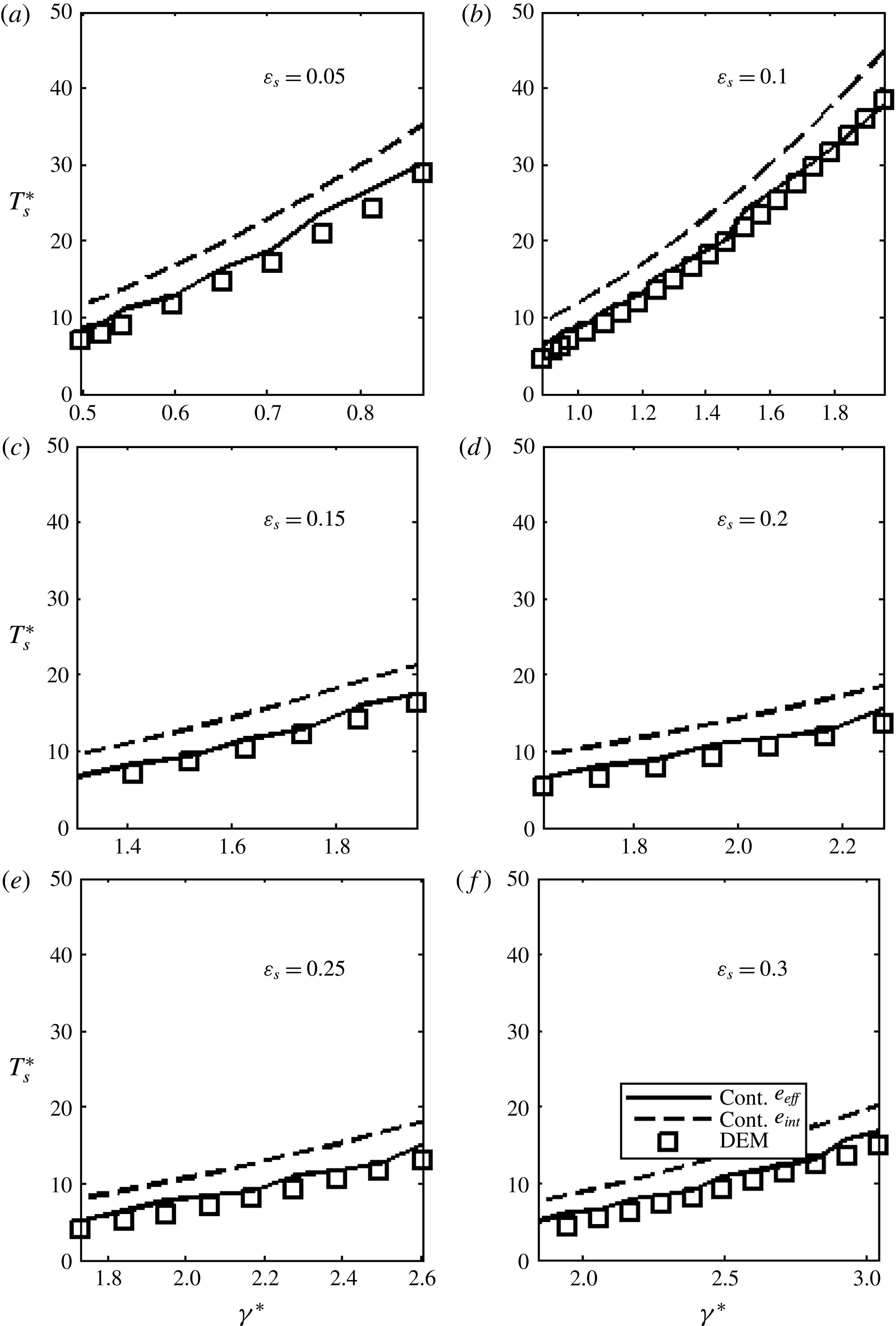
. Explicit closures can be found in detail elsewhere (e.g. Garzó & Dufty (Reference Garzó and Dufty1999) for a monodisperse system). In a cohesive system, agglomerate shape is expected to have an effect on these closures, which are based on an assumption of spherical particles. Rigorous inclusion of these effects is outside the scope of this work, and is not relevant for the lightly cohesive approximately monodisperse system examined here. Accordingly, the focus of kinetic-theory modifications considered here will remain on the effects of cohesion on the coefficient of restitution.
2.4 Closure of kinetic-theory-based balances: effective restitution coefficient
As discussed earlier, collisions between cohesive particles are more dissipative than collisions between non-cohesive particles due to the added acceleration experienced by approaching particles with attractive forces. For non-cohesive particles, the (intrinsic) coefficient of restitution is defined as the absolute value of the ratio of the post-collision normal relative velocity
 $v_{n,f}$
and the pre-collision normal relative velocity
 $v_{n,0}$
of two colliding particles
 $(e_{int}=|v_{n,f}/v_{n,0}|)$
, and is an input to the kinetic-theory-based closures for the transport coefficients. For elastic particles,
 $e_{int}=1$
, and for inelastic particles,
 $0<e_{int}<1$
. For cohesive particles, the additional dissipation decreases the value of
 $|v_{n,f}/v_{n,0}|$
to some effective value,
 $e_{eff}$
, which depends on the velocity at which the particles collide (Davis et al.
Reference Davis, Rager and Good2002; Donahue et al.
Reference Donahue, Hrenya, Davis, Nakagawa, Zelinskaya and Joseph2010; Gollwitzer et al.
Reference Gollwitzer, Rehberg, Kruelle and Huang2012; Abbasfard, Evans & Moreno-Atanasio Reference Abbasfard, Evans and Moreno-Atanasio2016); at infinitely high impact velocities,
 $e_{eff}\rightarrow e_{int}$
.
To account for cohesion, we seek to use an impact-velocity-dependent coefficient of restitution, ultimately cast in terms of its continuum counterpart
 $T_{s}$
. First, the dependence of
 $e_{eff}$
on
 $v_{n}$
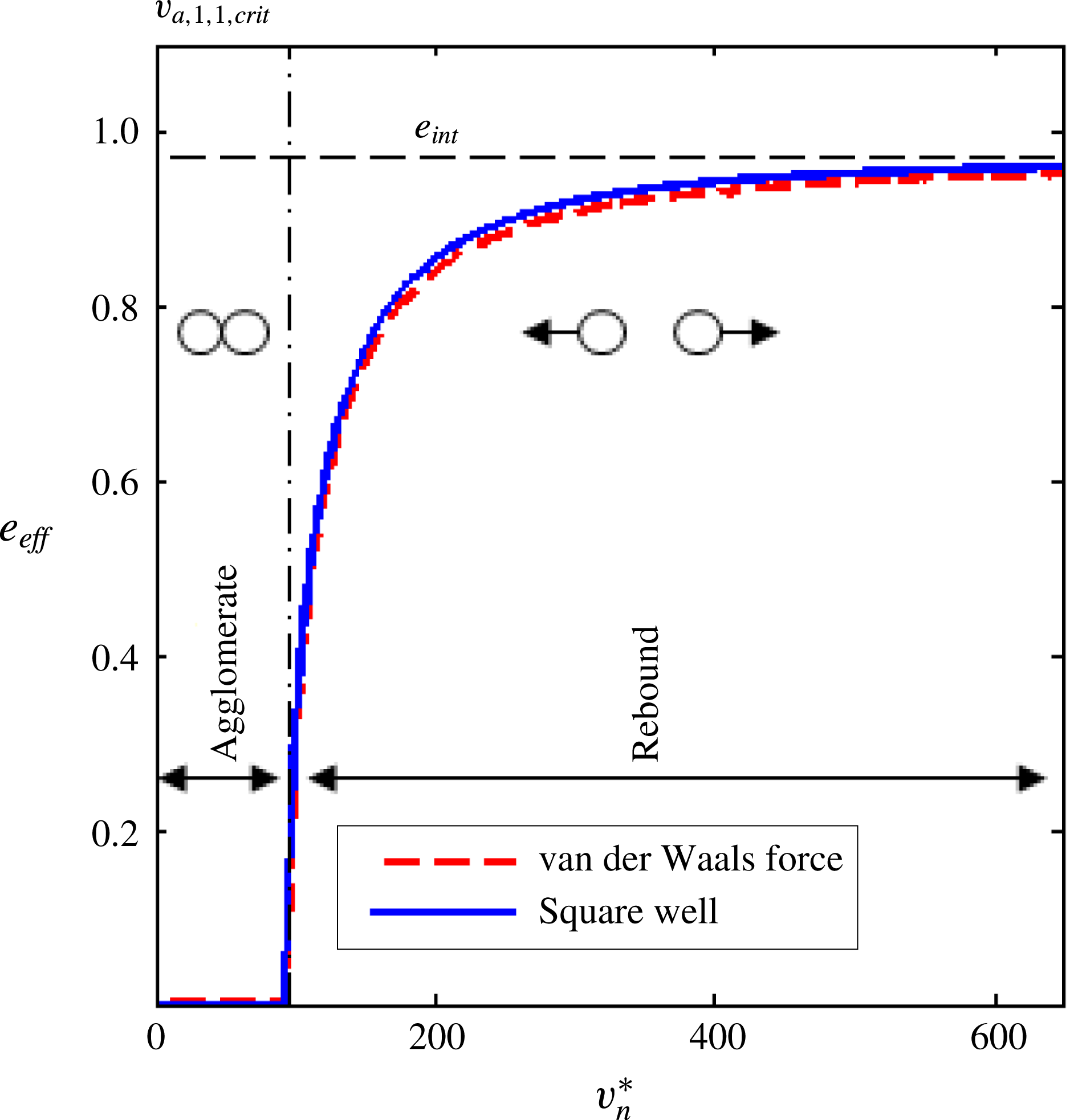
can be determined from experiments or DEM simulations; an illustrative example is shown in the dotted line of figure 4 for the case of van der Waals forces. Aggregation occurs when
 $e_{eff}=0$
and rebound occurs when
 $e_{eff}>0$
. This dependence can be captured via a numerical fit of the data from experiments or the DEM. Alternatively, an analytical approximation based on the square-well model is used here for purposes of simplicity. In particular, an analytical prediction for
 $e_{eff}$
is available for cohesive hard spheres described by a square well (Weber et al.
Reference Weber, Hoffman and Hrenya2004),
 $$\begin{eqnarray}e_{eff}(v_{n})=H(v_{n})\sqrt{e_{int}^{2}+\frac{(e_{int}^{2}-1)D_{well}}{4mv_{n}^{2}}},\end{eqnarray}$$
where
 $e_{int}$
is the intrinsic (non-cohesive) coefficient of restitution, assumed to be constant for this work, and
 $D_{well}$
is the well depth, given by Weber et al. (Reference Weber, Hoffman and Hrenya2004),
 $$\begin{eqnarray}D_{well}=\frac{4mv_{a,crit}^{2}e_{int}^{2}}{1-e_{int}^{2}}.\end{eqnarray}$$
Figure 4 shows a comparison of
 $e_{eff}$
predicted by the square-well model with that observed in two-particle simulations (DEM) of particles subject to van der Waals cohesion. The results indicate that the analytical prediction of
 $e_{eff}$
based on the square-well model agrees quantitatively well with the DEM data. Further, the expression for
 $e_{eff}(v_{n})$
given by the square-well model (2.36) is expected to be extendible to other types of cohesion where the
 $e_{eff}$
versus
 $v_{n}$
plot takes on the same general shape – e.g. liquid bridging experiments (Davis et al.
Reference Davis, Rager and Good2002; Weber et al.
Reference Weber, Hoffman and Hrenya2004; Liu et al.
Reference Liu, van Wachem, Mudde, Chen and van Ommen2016c
).
Effective coefficient of restitution measured in DEM simulations of collisions between two particles with van der Waals forces described in § 3.2.1 (red dashed line) compared with the prediction from the square-well model ((2.36), blue solid line), as well as the intrinsic property value (black dashed line).

Rigorous incorporation of an impact-velocity-dependent coefficient of restitution, as illustrated in figure 4, into the derivation of the transport coefficients is non-trivial at best even for simple systems (Murphy & Subramaniam Reference Murphy and Subramaniam2015), and is outside the current scope. Another approach to account for the additional dissipation due to cohesion is by using a mean value of the effective coefficient of restitution
 $e_{eff}$
, or
 $\langle e_{eff}\rangle$
, in the transport coefficients and dissipation rate. This value of
 $\langle e_{eff}\rangle$
, like
 $e_{eff}$
itself, lies in the range
 $0<\langle e_{eff}\rangle <e_{int}$
. Whereas Murphy & Subramaniam (Reference Murphy and Subramaniam2015) used
 $e_{eff}$
in the dissipation term in the granular energy balance, here,
 $\langle e_{eff}\rangle$
is instead calculated and utilized in all of the kinetic-theory-based closures. The mean effective coefficient of restitution is calculated via
 $$\begin{eqnarray}\langle e_{eff}\rangle =\frac{\displaystyle \int _{v_{a,crit}}^{\infty }e_{eff}(v_{n})f(v_{n})\,\text{d}v_{n}}{\displaystyle \int _{v_{a,crit}}^{\infty }f(v_{n})\,\text{d}v_{n}},\end{eqnarray}$$
where
 $f(v_{n})$
is defined above in terms of
 $T_{s}$
(see (2.31)) and
 $e_{eff}(v_{n})$
is dictated by the specific type of cohesion under consideration. It should be noted that this integrand has no analytical solution and must be integrated numerically for each numerical cell in the domain of a given system.
3 Methods
3.1 Discrete element method
An in-house code was used to perform the DEM simulations. The position
 $\boldsymbol{x}$
and velocity
 $\boldsymbol{v}$
of each particle were updated according to Newton’s second law of motion, using Euler integration. The forces acting on the particles are given by
 $$\begin{eqnarray}\boldsymbol{F}=\boldsymbol{F}_{coh}+\boldsymbol{F}_{cont}.\end{eqnarray}$$
Here,
 $\boldsymbol{F}$
is the sum of the cohesive
 $(\boldsymbol{F}_{coh})$
and contact
 $(\boldsymbol{F}_{cont})$
forces acting on the particle (no external forces are considered in this work). For simplicity, particle friction was not included in this study, and thus the angular momentum balance was not included.
The Hertzian contact model gives the magnitude of the contact force (Antypov & Elliott Reference Antypov and Elliott2011),
 $$\begin{eqnarray}F_{cont}=\left\{\begin{array}{@{}ll@{}}\displaystyle \frac{4E_{eff}\sqrt{R_{eff}}}{3}\unicode[STIX]{x1D6FF}^{3/2}+\unicode[STIX]{x1D702}\,\frac{\text{d}\unicode[STIX]{x1D6FF}}{\text{d}t}, & \unicode[STIX]{x1D6FF}\geqslant 0,\\ 0, & \unicode[STIX]{x1D6FF}<0,\end{array}\right.\end{eqnarray}$$
where
 $\unicode[STIX]{x1D6FF}$
is the overlap of the two particles and
 $$\begin{eqnarray}\displaystyle & \displaystyle E_{eff}=\frac{E_{i}E_{j}}{E_{i}(1+\unicode[STIX]{x1D708}_{j}^{2})+E_{j}(1+\unicode[STIX]{x1D708}_{i}^{2})}, & \displaystyle\end{eqnarray}$$
 $$\begin{eqnarray}\displaystyle & \displaystyle R_{eff}=\frac{R_{i}R_{j}}{R_{i}+R_{j}}, & \displaystyle\end{eqnarray}$$
 $$\begin{eqnarray}\displaystyle & \displaystyle \unicode[STIX]{x1D702}=\frac{-2\sqrt{15m_{eff}E_{eff}}R_{eff}^{1/4}\ln (e_{int})}{3\sqrt{\unicode[STIX]{x03C0}^{2}+\ln ^{2}(e_{int})}}\unicode[STIX]{x1D6FF}^{1/4}, & \displaystyle\end{eqnarray}$$
where the subscripts
 $i$
and
 $j$
represent denote the properties of each of the contacting particles,
 $E$
is Young’s modulus,
 $e_{int}$
is the intrinsic coefficient of restitution and the effective mass is
 $$\begin{eqnarray}m_{eff}=\frac{m_{i}m_{j}}{m_{i}+m_{j}}.\end{eqnarray}$$
A cohesion model that accounts for van der Waals forces is used in this work for the purposes of illustration, although other cohesion models can be used to develop the cohesion-specific closures for the continuum theory. Here, a modified two-scale Rabinovich et al. (Reference Rabinovich, Adler, Ata, Singh and Moudgil2000) theory was used to estimate van der Waals forces. This theory accounts for cohesion between all combinations of large- (
 $L$
) and small- (
 $S$
) scale roughness on both particles. The magnitude of the force between particles
 $i$
and
 $j$
is given by Liu et al. (Reference Liu, LaMarche, Kellogg and Hrenya2016b
),
 $$\begin{eqnarray}\displaystyle & & \displaystyle F_{coh}(D>D_{min})=\frac{A}{6}\left[\frac{R_{i}R_{j}}{(R_{i}+R_{j})(D+y_{iL}+y_{jL}+y_{iS}+y_{jS})^{2}}\right.\nonumber\\ \displaystyle & & \displaystyle \quad +\,\frac{R_{i}r_{jL}}{(R_{i}+r_{jL})(D+y_{iL}+y_{iS}+y_{jS})^{2}}\nonumber\\ \displaystyle & & \displaystyle \quad +\,\frac{R_{i}r_{jS}}{(R_{i}+r_{js})(D+y_{iL}+y_{iS})^{2}}+\frac{r_{iL}R_{i}}{(r_{iL}+R_{j})(D+y_{iS}+y_{jL}+y_{jS})^{2}}\nonumber\\ \displaystyle & & \displaystyle \quad +\,\frac{r_{iL}r_{jL}}{(r_{iL}+r_{jL})(D+y_{iS}+y_{jS})^{2}}+\frac{r_{iL}r_{jS}}{(r_{iL}+r_{jS})(D+y_{iS})^{2}}\nonumber\\ \displaystyle & & \displaystyle \quad \left.+\,\frac{r_{iS}R_{j}}{(r_{iS}+R_{j})(D+y_{iL}+y_{jS})^{2}}+\frac{r_{iS}r_{jL}}{(r_{iL}+r_{jL})(D+y_{jS})^{2}}+\frac{r_{iS}r_{jS}}{(r_{iS}+r_{jS})D^{2}}\right],\end{eqnarray}$$
 $$\begin{eqnarray}r_{kl}=\frac{\unicode[STIX]{x1D706}_{kl}^{2}}{32k_{1}rms_{kl}},\quad y_{kl}=k_{1}rms_{kl},\end{eqnarray}$$
where
 $\unicode[STIX]{x1D706}$
is the wavelength of the roughness,
 $k_{1}=1.817$
is a geometric constant,
 $rms_{kl}$
is the root mean square height of asperities,
 $r_{kl}$
is the radius of asperities and
 $y_{kl}$
is the asperity height, with the subscript
 $k$
taking values of
 $i$
or
 $j$
and the subscript
 $l$
taking values of
 $S$
or
 $L$
. Here,
 $A$
is the Hamaker constant,
 $R$
is the particle radius,
 $D$
is the distance between the highest asperity of the two particles and
 $D_{min}$
is the cutoff distance, frequently taken to be the intermolecular separation distance. When particles are separated by less than the minimum cutoff distance,
 $$\begin{eqnarray}F_{coh}(D\leqslant D_{min})=F_{coh}(D_{min}).\end{eqnarray}$$
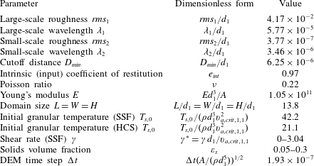
The values of the particle properties for this cohesive model are summarized in table 1. The values used correspond to glass beads, similar to those used in previous experiments (LaMarche et al. Reference LaMarche, Leadley, Liu, Kellogg and Hrenya2017).
The dimensionless input parameters (particle and system) used in the DEM simulations.

3.2 Systems examined
Discrete element method simulations were used both to extract the cohesion-specific quantities (
 $v_{a,crit}$
,
 $v_{b,crit}$
,
 $d_{V,V^{\prime }}$
and
 $e_{eff}$
) and to validate the continuum theory. Since a lightly cohesive system is considered here (only singlets and doublets), only one distribution of daughters (
 $b$
) is possible (two singlets), thereby precluding the need to determine this quantity. Different systems were utilized for these purposes, as described below.
3.2.1 Controlled two-particle DEM
Controlled two-particle DEM simulations were utilized to determine the critical velocity of aggregation for singlet–singlet collisions
 $v_{a,1,1,crit}$
, as needed to evaluate the success factor of aggregation
 $\unicode[STIX]{x1D713}_{a}$
(2.11) and the effective coefficient of restitution
 $e_{eff}$
(2.38). Namely, simulations of two particles colliding at various impact angles and velocities were performed to determine whether aggregation or rebound occurred. This two-particle system was chosen to determine
 $v_{a,1,1,crit}$
for colliding singlets, as singlet–singlet collisions have limited orientations and the full parameter space is easily covered. (Nonetheless, it should be recalled that the normal critical velocity of aggregation was found to be independent of the collision orientation, as shown in figure 1.)
Controlled DEM simulations were not used to determine the critical velocity of breakage
 $v_{b,1,2,crit}$
, nor the collision cylinder diameter
 $d_{1,2}$
, however, as the parameter space of collisions involving doublets becomes quite large with the inclusion of added parameters – e.g. orientation and rotation speed of the doublet at time of collision (Liu et al.
Reference Liu, Kellogg, LaMarche and Hrenya2017). Further, if the simulation is extended to consider collisions with larger agglomerates, additional parameters such as the packing of agglomerate (compact versus loose) and agglomerate shape must be considered. Perhaps more importantly, we found via such controlled DEM simulations that
 $v_{b,1,2,crit}$
depends on the collision orientation and gives rise to some outlier values. Direct account for the dependence of
 $v_{b,1,2,crit}$
on the impact orientation is not possible in the continuum framework since this quantity not known a priori or solved for. Thus, as a first step, we use a constant mean value of
 $v_{b,1,2,crit}$
in this work. Moreover, the collision orientations associated with outlier values of
 $v_{b,1,2,crit}$
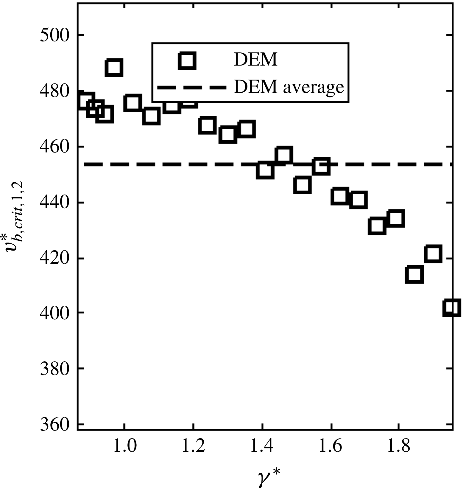
observed in controlled DEM simulations were seldom seen to occur in the many-particle flow systems considered here, although they greatly influence the mean critical velocity extracted from a range of collision orientations. Therefore, generally speaking, it is important to determine the critical velocity of breakage, the critical velocity of aggregation for agglomerates, the collision cylinder diameters and the daughter distributions from such many-particle flows, where these outlier collisions are infrequent. In the work described herein, we will use many-particle SSF simulations to determine
 $v_{b,1,2,crit}$
since shear is often present in practical cohesive flows.
3.2.2 Simple shear flow
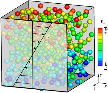
Simple shear flow was achieved via periodic walls on four sides of the domain. The remaining two opposite sides were simulated using Lees–Edwards boundary conditions, which impose a constant velocity gradient (Lees & Edwards Reference Lees and Edwards1972), as shown in figure 5. The domain was chosen to have dimensions of
 $L/d=13.8$
in order to prevent clustering instabilities (see (Fullmer & Hrenya Reference Fullmer and Hrenya2017) for a review), which would cause the system to become inhomogeneous and thus complicate the prediction of the local granular temperatures and success factors. Preliminary simulations of the SSF system indicated that at low initial granular temperatures and/or low shear rates, the system evolves into one large agglomerate. Therefore, the SSF simulations were initialized with a granular temperature much greater than the steady-state value, and using (higher) shear rates that lead to a distribution of agglomerate sizes. Particles were initialized at random locations within the domain, with fluctuating velocities determined by a Maxwellian distribution, where the mean velocity was given by the imposed shear velocity at that location and the variance given by the initial granular temperature. For both the SSF and HCS, replicate DEM simulations with different random seed initial conditions showed little sensitivity in the results explored to the initial conditions. These simulations approached a steady state by
 $t^{\ast }=t(A/(\unicode[STIX]{x1D70C}d_{1}^{5}))^{1/2}\sim 2$
(where
 $\unicode[STIX]{x1D70C}$
is the particle density,
 $A$
is the Hamaker constant and
 $d_{1}$
is the diameter of a singlet) and were continued until a dimensionless time of
 $t^{\ast }\sim 10$
in order to collect adequate statistics. Only (statistical) steady-state values were utilized in the analysis of this system.
Simple shear flow simulations were used to determine the critical velocity of breakage
 $v_{b,1,2,crit}$
between a singlet and a doublet as well as the collision cylinder diameter
 $d_{1,2}$
. More specifically,
 $v_{b,1,2,crit}$
was determined by extracting the success factor of breakage
 $\unicode[STIX]{x1D713}_{b}$
as well as the granular temperature
 $T_{s}$
from the DEM simulations, and then calculating the critical velocity of breakage according to (2.12),
 $$\begin{eqnarray}\unicode[STIX]{x1D6F9}_{b}(1,2)=\int _{v_{b,1,2,crit}}^{\infty }f(v_{n})\,\text{d}v_{n}=\exp \left[\frac{-v_{b,1,2,crit}^{2}}{2T_{s}\displaystyle \left[\frac{1}{m_{1}}+\frac{3}{m_{2}5}\right]}\right],\end{eqnarray}$$
where
 $m_{1}$
and
 $m_{2}$
are the masses of singlets and doublets, respectively.
Schematic of an SSF system in the DEM. The transparent front pane shows the mean velocity profile.

Simple shear flow simulations were also used to determine the collision cylinder diameter for singlet–doublet collisions
 $d_{1,2}$
(distance between the centres of the agglomerate and the colliding singlet particles) used in the breakage kernel for doublets (3.10). This parameter is directly related to the projected sweep area of a doublet, and consequently influences the frequency of collisions.
Daughter distributions can be estimated determined from DEM SSF simulations, but are not required for the lightly cohesive system considered here, as the largest agglomerates considered are doublets, which always produce two singlets when broken.
3.2.3 Homogeneous cooling system
For the purposes of initial validation studies of the new continuum theory, the HCS was utilized. The HCS was transient, with the state of the system approaching one large agglomerate with a near-zero granular temperature. Periodic walls were utilized on all sides, and the system was initially (approximately) homogeneous, with no net momentum and no external forces. These simulations were arbitrarily initialized with the granular temperature given in table 1. Because the focus here is on validating the approach for a lightly cohesive system where only singlets and doublets are present, simulation results were only considered up to the time when 3 % of the particles were in agglomerates larger than doublets. Moreover, it should be noted that the distribution of collision orientations in the HCS differs from that of SSF, so this system will be used to make a first assessment of the validity of using a mean value of
 $v_{b,1,2,crit}$
determined from SSF.
3.2.4 Agglomerate detection and simulation parameters
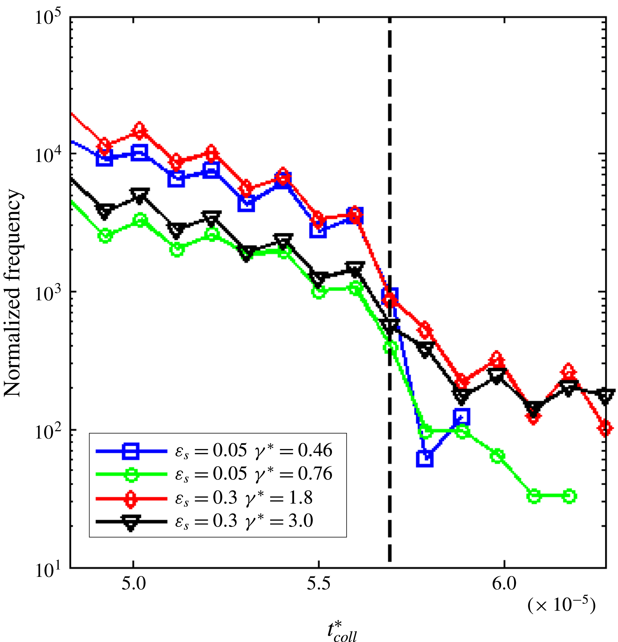
Agglomerates in the DEM simulations were detected using a method that records the collision duration between individual particles. Figure 6 demonstrates a steep drop-off in the frequency of collision duration for the SSF systems examined here and outlined in table 1. This drop-off forms a boundary between shorter collisions that correspond to particles rebounding from non-agglomerating collisions, and longer collisions that correspond to particles agglomerating. A critical collision duration of
 $t_{crit}^{\ast }=t_{coll}(A/(\unicode[STIX]{x1D70C}d_{1}^{5}))^{1/2}\sim 5.7\times 10^{-5}$
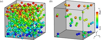
(dashed black line) was chosen for agglomerate detection, as this corresponds to the steep drop-off over a wide range of system parameters. Particles in contact for longer than this critical value were identified as agglomerates. This agglomerate detection algorithm is demonstrated in figure 7. Figure 7(a) shows all of the particles in a cohesive DEM SSF. In figure 7(b), only the agglomerates detected in figure 7(a) are shown.
3.3 Continuum theory
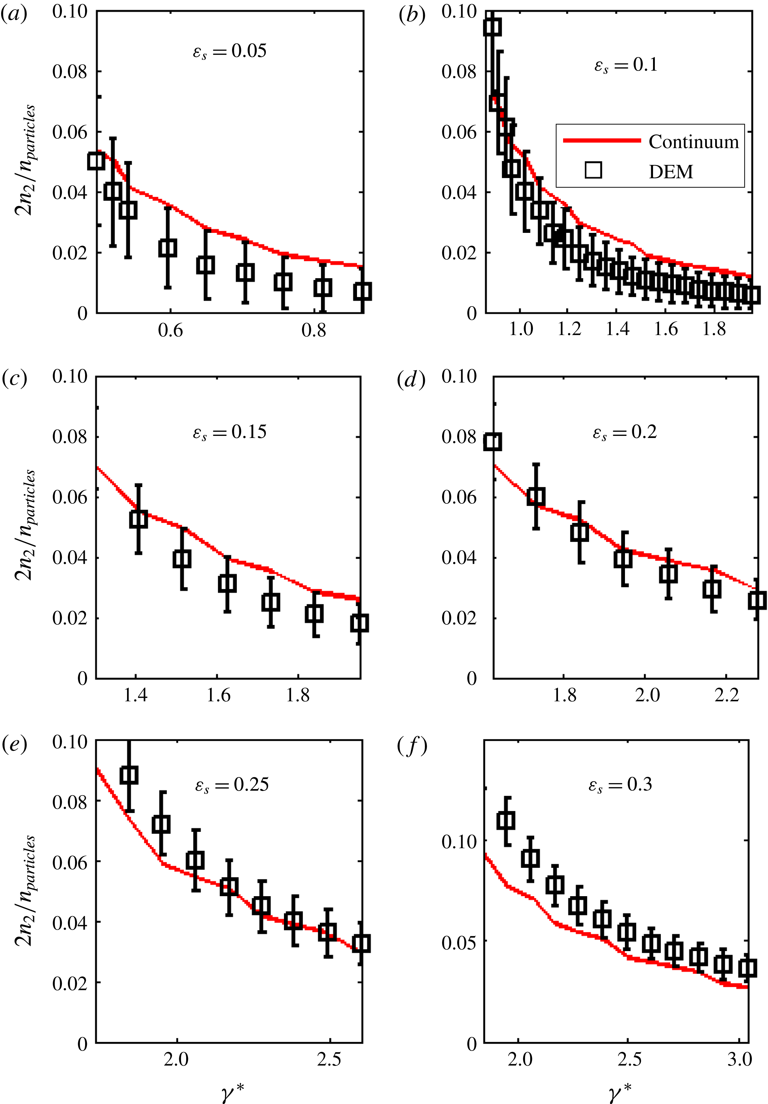
The continuum theory, namely the population balance and granular energy balances, was used to predict the number density of particles in singlets (
 $n_{1}$
) and doublets (
 $n_{2}$
), along with the (statistically steady) granular temperature (
 $T_{s}$
) for SSF. The continuum theory was also used to solve for
 $n_{1}$
,
 $n_{2}$
and
 $T_{s}$
as they evolved in time for the HCS. The initial conditions of the HCS and SSF continuum simulations were identical to those used in the DEM.
Frequency of non-dimensional collision durations
 $(t_{coll}^{\ast }=t_{coll}(A/(\unicode[STIX]{x1D70C}d_{1}^{5}))^{1/2})$
in a wide range of cohesive DEM SSF simulations. The dashed black line shows the threshold for agglomerate detection. The results are normalized by the number of collisions that occurred in each simulation.

Although a polydisperse kinetic theory may be more appropriate for a system with a broad distribution of agglomerate sizes, the focus here is on the closure of the population balance for a lightly cohesive system dominated by singlets and doublets, with mostly singlets (i.e. not a broad distribution of agglomerate sizes). Thus, the monodisperse kinetic theory given by Garzó & Dufty (Reference Garzó and Dufty1999) was used to provide the closures for the solid stress and the dissipation rate based on a particle size/mass equal to that of a primary particle. It should also be noted that for the SSF and HCS explored here, no slip velocity exists between the different agglomerate sizes (i.e.
 $|\boldsymbol{u}_{\boldsymbol{V}}-\boldsymbol{u}_{\boldsymbol{V}^{\prime }}|=0$
). In other systems where slip does exist between the different agglomerate sizes, a polydisperse kinetic theory that takes into account the effect of the slip on the collision frequency must be used (Garzó et al.
Reference Garzó, Dufty and Hrenya2007a
,Reference Garzó, Hrenya and Dufty
b
; Hrenya Reference Hrenya2011). The assumption that a monodisperse kinetic theory is applicable here will be checked later. Further, the granular energy was assumed to be equal for all agglomerate sizes (equipartition of energy), and thus only one granular energy balance was required.
(a) Snapshot of a cohesive DEM SSF system with all of the particles present
 $(\unicode[STIX]{x1D700}_{s}=0.10,\unicode[STIX]{x1D6FE}^{\ast }\sim 0.90)$
. (b) Snapshot of only the agglomerates detected in (a).

3.3.1 Simple shear flow
For a homogeneous SSF system, the population balances (2.1), (2.3), (2.5), (2.7) reduce to
 $$\begin{eqnarray}0=-2\unicode[STIX]{x1D6FD}_{1,1}n_{1}n_{1}+2\unicode[STIX]{x1D6FC}_{1,2}n_{1}n_{2},\end{eqnarray}$$
where
 $n_{1}$
and
 $n_{2}$
are the number densities of singlets and doublets,
 $\unicode[STIX]{x1D6FD}_{1,1}$
is the aggregation kernel of singlets and
 $\unicode[STIX]{x1D6FC}_{1,2}$
is the breakage kernel of doublets due to collisions with singlets. The granular energy balance reduces to
 $$\begin{eqnarray}0=\frac{2}{3n_{particles}}\unicode[STIX]{x1D707}\unicode[STIX]{x1D6FE}^{2}-\unicode[STIX]{x1D701}T_{s},\end{eqnarray}$$
where
 $T_{s}$
is the granular temperature,
 $\unicode[STIX]{x1D707}$
is the granular shear viscosity,
 $n_{particles}$
is the total number density of (primary) particles in the system,
 $\unicode[STIX]{x1D6FE}$
is the shear rate and
 $\unicode[STIX]{x1D701}$
is the dissipation coefficient. Here,
 $\unicode[STIX]{x1D701}$
and
 $\unicode[STIX]{x1D707}$
were determined by substituting the mean effective coefficient of restitution (
 $\langle e_{eff}\rangle$
; see (2.38)) in place of the (intrinsic) coefficient of restitution in the constitutive relations given by Garzó & Dufty (Reference Garzó and Dufty1999). The first term on the right-hand side of the equation represents the generation of granular energy due to shear and the second term represents the dissipation of granular energy due to inelastic collisions. It is worthwhile to note that only one-way coupling is present between the population and granular energy balances – i.e. the granular temperature can be solved independently of the population balances, but not vice versa, since
 $\unicode[STIX]{x1D6FC}_{1,2}=f(T_{s})$
.
Each combination of shear rate and solids volume fraction represents an independent simulation (i.e. each DEM data point (figures 8–13) represents an independent simulation with a different random initial condition). The error bars shown on these figures for the DEM results reflect the standard deviation after steady state is reached. Similarly, a corresponding continuum solution was obtained for each condition simulated via the DEM.
3.3.2 Homogeneous cooling system
For the HCS, the population balances are identical to those of SFF, except with time derivative terms included, as the system is transient,
 $$\begin{eqnarray}\displaystyle & \displaystyle \frac{\text{d}n_{1}}{\text{d}t}=-2\unicode[STIX]{x1D6FD}_{1,1}n_{1}n_{1}+2\unicode[STIX]{x1D6FC}_{1,2}n_{1}n_{2}, & \displaystyle\end{eqnarray}$$
 $$\begin{eqnarray}\displaystyle & \displaystyle \frac{\text{d}n_{2}}{\text{d}t}=\unicode[STIX]{x1D6FD}_{1,1}n_{1}n_{1}-\unicode[STIX]{x1D6FC}_{1,2}n_{1}n_{2}. & \displaystyle\end{eqnarray}$$
In the absence of shear, the granular energy balance further reduces to
 $$\begin{eqnarray}\frac{\text{d}T_{s}}{\text{d}t}=-\unicode[STIX]{x1D701}T_{s},\end{eqnarray}$$
where the dissipation of granular energy in time is dictated by inelastic collisions. Similarly to the SSF system, only one-way coupling exists between the granular energy and the population balances for the homogeneous cooling simulations. The population and granular energy balance equations were solved until 3 % of the particles were in agglomerates larger than doublets.
Five independent DEM simulations (with different random initial conditions) were performed for each solids volume fraction in the HCS. The error bars shown in figures 14 and 15 indicate the standard deviation of the DEM results from these five independent simulations. A single continuum solution was found for each solids volume fraction.
3.3.3 Numerical solution
Using an in-house MatLab script, an implicit Euler time march was used to solve the transient population and energy balances for the HCS simulations. For the SSF simulations, the transient terms were reintroduced, and the same implicit Euler time march was used to relax the agglomerate size distributions and granular temperatures to the steady-state solutions (i.e. the transient terms approached zero, consistent with (3.11)–(3.12)). For both systems, an adjustable time step was used to overcome initial stiffness in the system. To ensure numerical accuracy, insensitivity to the time step and residual values was confirmed for a few test cases encompassing the parameter space.
4 Results and discussion
4.1 Extraction of cohesion-specific quantities needed for continuum-theory closures: collision cylinder diameter and critical velocities
Three quantities were extracted from DEM simulations for use in the continuum theory: the collision cylinder diameter for singlet–doublet collisions,
 $d_{V,V^{\prime }}$
(via SSF), the critical velocity of aggregation for singlet–singlet collisions,
 $v_{a,1,1,crit}$
(via controlled two-particle collisions), and the critical velocity of breakage for singlet–doublet collisions,
 $v_{b,1,2,crit}$
(via SSF). The results for these cohesion-specific quantities are summarized in table 2. For the lightly cohesive system explored here, doublet–doublet collisions were neglected because the low concentration of doublets led to a very low frequency of doublet–doublet collisions relative to singlet–doublet collisions, thus making the breakage of doublets due to these types of collisions negligible.
The quantity
 $d_{V,V^{\prime }}$
was determined by averaging the distance between the centre of the doublet and the centre of the singlet for collisions of singlets and doublets detected in SSF simulations. The quantity
 $v_{a,1,1,crit}$
was measured using controlled two-particle DEM simulations (see figure 1).
Cohesion-specific quantities extracted from DEM SSF simulations and used as inputs to continuum SSF and HCS simulations.

As described in § 3.2.2,
 $v_{b,1,2,crit}$
was determined from the measured success factors of breakage
 $\unicode[STIX]{x1D713}_{b}$
in DEM SSF and using the closure for the success factor of breakage given in (2.12). The value of
 $v_{b,1,2,crit}$
shows a slight downward trend as the shear rate
 $\unicode[STIX]{x1D6FE}^{\ast }$
increases; see figure 8. A plausible explanation for this observation is the following: as the shear rate increases, agglomerate rotation increases, thus making it easier for agglomerates to break (the rotational motion adds to the normal impact velocity due to translational motion alone). Additional simulations for different values of
 $v_{b,1,2,crit}$
across the range measured in figure 8 were performed, and
 $\unicode[STIX]{x1D713}_{b,1,2}$
was found to be insensitive to
 $v_{b,1,2,crit}$
in this range, so use of a mean value in the continuum theory was deemed to be acceptable.
4.2 Verification and validation of continuum theory: SSF
Simple shear flow was first used to validate the closure for the success factor of aggregation
 $\unicode[STIX]{x1D713}_{a}$
(2.11) and then to validate the closure for
 $\langle e_{eff}\rangle$
(2.38). As detailed below, the corresponding comparisons with quantities extracted from DEM simulations constitute validation (theory, or closure, accuracy) rather than verification (code accuracy) (Grace & Taghipour Reference Grace and Taghipour2004) since
 $\unicode[STIX]{x1D713}_{a}$
and
 $\langle e_{eff}\rangle$
depend only on the critical velocity of aggregation
 $v_{a,1,1,crit}$
determined from DEM simulations of controlled two-particle collisions (rather than SSF). Next, SSF was used for verification (code accuracy) of the aggregation and breakage kernels (2.8)–(2.9). This last comparison is verification (code accuracy) rather than validation (theory accuracy), as the cohesion-specific inputs of the critical velocity of breakage
 $v_{b,1,2,crit}$
and the collision cylinder diameter
 $d_{V,V^{\prime }}$
, which were determined from the SSF system, were subsequently used in the continuum-theory predictions for SSF. Further, these latter verifications utilized
 $n_{1}$
,
 $n_{2}$
and
 $T_{s}$
extracted from the DEM simulations, rather than the predicted values, to ensure that any resulting discrepancies were traceable directly to the aggregation and breakage kernels themselves.
Critical velocity of breakage calculated from DEM SSF simulations with
 $\unicode[STIX]{x1D700}_{s}=0.1$
(black points). The dashed line shows the mean value used in continuum theory.

It should be recalled that the success factor
 $\unicode[STIX]{x1D713}_{a,1,1}$
is used to determine the rate of aggregation in the system (2.3), and is therefore a key quantity for the accurate prediction of the agglomerate size distributions
 $n_{1}$
and
 $n_{2}$
. For simple shear flow,
 $\unicode[STIX]{x1D713}_{a,1,1}$
was extracted directly from the DEM, and compared with the current theory (2.11), as well as a previous theoretical expression (Liu Reference Liu2011). Both of these theoretical expressions depend on
 $v_{a,1,1,crit}$
and
 $T_{s}$
. It should be recalled that the value of
 $v_{a,1,1,crit}$
for these predictions was determined from controlled two-particle DEM simulations, and the value of
 $T_{s}$
used in the prediction was extracted directly from the DEM SSF simulations in order to isolate any discrepancies as stemming from the closure for
 $\unicode[STIX]{x1D713}_{a,1,1}$
, rather than uncertainty in
 $T_{s}$
. Figure 9 demonstrates that the new theory outlined here correctly predicts the success factor measured via the DEM, whereas the previous theory of Liu (Reference Liu2011) significantly underpredicts
 $\unicode[STIX]{x1D713}_{a,1,1}$
. In the current theory,
 $\unicode[STIX]{x1D713}_{a,1,1}$
is determined from the distribution of normal impact velocities. The disagreement between
 $\unicode[STIX]{x1D713}_{a,1,1}$
predicted by the Liu theory (Reference Liu2011) and the DEM simulation results is not surprising since the value of
 $\unicode[STIX]{x1D713}_{a,1,1}$
in the Liu theory (Reference Liu2011) is determined from the distribution of total impact velocities (including tangential components). These results are consistent with figure 3. That is, at lower impact velocities, the probability of an impact having a given total relative velocity as predicted by the Liu theory (Reference Liu2011) is much smaller than the probability of a collision having the same given normal relative impact velocity as predicted by the current theory. Integration of these impact velocity distributions from 0 to a constant
 $v_{a,1,1,crit}$
to determine
 $\unicode[STIX]{x1D713}_{a,1,1}$
(2.11) causes the Liu theory (Reference Liu2011) to underpredict
 $\unicode[STIX]{x1D713}_{a,1,1}$
, as evidenced in figure 9. It should also be noted that for the limiting case of aggregation between singlets, the prediction of
 $\unicode[STIX]{x1D713}_{a,1,1}$
given by the current model is consistent with the ratio of the frequency of collisions that successfully result in agglomeration to the total collision frequency predicted by Murphy & Subramaniam (Reference Murphy and Subramaniam2015).
Success factor of aggregation for
 $\unicode[STIX]{x1D700}_{s}=0.1$
. The solid line shows the prediction by Liu (Reference Liu2011).

Another closure that can be validated directly via SSF simulations is the kinetic-theory treatment involving
 $\langle e_{eff}\rangle$
. For SSF, the momentum balances are solved identically such that only the energy balance and population balance require solution. It should be recalled that the granular energy balance has one-way coupling with the population balance, such that the granular energy balance affects the population balance, but not vice versa. Therefore, the granular energy balance can be solved in isolation for
 $T_{s}$
, and any discrepancies between the predicted value and that extracted from the DEM will arise from the kinetic-theory treatment itself (i.e.
 $\langle e_{eff}\rangle$
), and not due to the new closures in the population balance. A comparison between the
 $T_{s}$
measured in the DEM and that predicted by the granular energy balance is given in figure 10. The kinetic theory for a non-cohesive system (using the intrinsic property for the coefficient of restitution
 $e_{int}$
in the dissipation and shear viscosity closures in the granular energy balance (3.14)) is included for comparison with the current (cohesive) theory and DEM simulations. The kinetic theory using
 $e_{int}$
gives an overestimation of the granular temperature compared with when
 $\langle e_{eff}\rangle$
is used. The excellent agreement between the DEM results and the kinetic-theory treatment using
 $\langle e_{eff}\rangle$
provides initial validation for this approach, and also provides support for the monodisperse assumption. Further, this approach gives an excellent prediction of the
 $T_{s}$
for a system outside of that explored by Murphy & Subramaniam (Reference Murphy and Subramaniam2015), which included the effect of
 $e_{eff}$
(rather than
 $\langle e_{eff}\rangle$
used here) in the dissipation term only, and was thus restricted to the HCS. Further, the approach used by Murphy & Subramaniam (Reference Murphy and Subramaniam2015) does not include the shear term (i.e. granular shear viscosity
 $\unicode[STIX]{x1D707}$
, which also depends on
 $e_{eff}$
) included here.
Comparison of the non-dimensional granular temperature
 $(T_{s}^{\ast }=T_{s}/(\unicode[STIX]{x1D70C}d_{1}^{3}v_{a,1,1,crit}^{2}))$
predicted in SSF by the continuum theory and the DEM for various solids volume fractions and shear rates. The continuum predictions are given by solid lines. The dashed line corresponds to a simulation using the intrinsic, rather than effective, coefficient of restitution. Points represent DEM data.

Comparison of the fraction of particles in doublets predicted in SSF by the continuum theory (solid lines) and the DEM (points) for various solids volume fractions and shear rates. The error bars show the standard deviation of the fraction of particles at incremental times after steady state was reached for one simulation.

Terms associated with aggregation and breakage rates for
 $\unicode[STIX]{x1D700}_{s}=0.1$
for (a–c) singlet–singlet interactions and (d–f) singlet–doublet interactions. Collision frequencies and aggregation and breakage rates are non-dimensionalized by multiplying by
 $d_{1}^{4}/v_{a,1,1,crit}$
.

Above, the closures of the new continuum theory that can be validated using SSF (
 $\unicode[STIX]{x1D713}_{a}$
and
 $\langle e_{eff}\rangle$
) are compared successfully with the DEM simulations (theory accuracy); we will now turn our attention to the remaining closures for which verification (code accuracy) can be carried out in SSF, and then move on to the HCS for validation of the same quantities. In particular, for verification purposes, the fraction of particles in doublets
 $(2n_{2}/n_{particles})$
predicted by the continuum theory (solution of both the kinetic theory and population balances) for SSF is compared with the DEM results. This comparison is verification since the critical velocity of breakage
 $v_{b,1,2,crit}$
was determined from the SSF DEM simulations, and this value is then used in the calculation of the fraction of particles in doublets (2.1). The resulting comparisons are shown in figure 11 for a range of concentrations and shear rates. The DEM simulations display a trend of a decreasing fraction of particles in doublets with an increasing shear rate. The same behaviour is captured by the continuum theory. This behaviour is expected, as an increased shear rate leads to an increased (steady state)
 $T_{s}$
. An increased
 $T_{s}$
(i.e. impact velocity) decreases the likelihood of agglomeration (
 $\unicode[STIX]{x1D713}_{a,1,1}$
) and increases the likelihood of breakage (
 $\unicode[STIX]{x1D713}_{b,1,2}$
), leading to less aggregation and more breakage, and thus fewer doublets.
Quantitatively, a non-systematic deviation exists between the fraction of particles in doublets observed in the DEM and the continuum-theory prediction (figure 11). More specifically, the continuum theory overpredicts the amount of aggregation in some cases (for all shear rates for
 $\unicode[STIX]{x1D700}_{s}=0.05$
, for most shear rates at
 $\unicode[STIX]{x1D700}_{s}=0.1{-}0.2$
) and underpredicts for other conditions (the lowest shear rates at
 $\unicode[STIX]{x1D700}_{s}=0.1{-}0.25$
and for all shear rates at
 $\unicode[STIX]{x1D700}_{s}=0.3$
). To identify the source of this deviation, the individual terms in the population balance are considered. In particular, the success factors of aggregation and breakage, the collision frequencies of singlet–singlet and singlet–doublet collisions, and the aggregation and breakage rates are considered individually in figure 12 for the case of
 $\unicode[STIX]{x1D700}_{s}=0.1$
. Namely, the product of the success factors (a,d) with the collision frequency (b,e) gives the rates of aggregation and breakage (c,f). Panels (a–c) represent singlet–singlet collisions and (d–f) represent singlet–doublet collisions.
The results for the different terms in the population balance shown in figure 12 explain the overprediction of the fraction of particles in doublets observed in figure 11 for
 $\unicode[STIX]{x1D700}_{s}=0.1$
. More specifically, figure 12(a) demonstrates that the continuum theory overpredicts the success factor
 $\unicode[STIX]{x1D713}_{a,1,1}$
(except at shear rates greater than
 $\unicode[STIX]{x1D6FE}^{\ast }\sim 1.6$
) and consequently the singlet–singlet aggregation rate in figure 12(c). Further, the continuum theory slightly underpredicts the collision frequency of singlet–doublet collisions
 $N_{1,2}$
(figure 12
e) for all shear rates, which causes a small underprediction in the breakage rate of doublets (figure 12
f). Collectively, these effects lead to an overprediction of particles in doublets for higher shear rates (figure 11
b), which explains the deviation between the continuum theory and the DEM observed for shear rates greater than
 $\unicode[STIX]{x1D6FE}^{\ast }\sim 0.98$
in figure 11(b). In figure 11(b), however, the continuum theory appears to accurately predict the fraction of particles in doublets at the lowest shear rates of
 $\unicode[STIX]{x1D6FE}^{\ast }\sim 0.87{-}0.98$
. One possible explanation for the absence of the expected mismatch is that the continuum theory is missing a sink of doublets, which would counteract the overprediction expected from figure 12(c,f).
To explain the discrepancy noted above, it is hypothesized that the birth of larger agglomerates (larger than doublets) due to aggregation may provide the missing net sink of doublets. Indeed, figure 13 indicates that larger agglomerates are present, especially at lower shear rates. More specifically, the doublet fraction in the DEM was observed to remain at a statistical steady state in time, requiring that the net source of doublets be zero. However, calculations confirm that an estimate of the net source of doublets observed in the DEM
 $(\unicode[STIX]{x1D700}_{s}=0.1)$
, based only on the aggregation rate of singlets less the breakage rate of doublets, is indeed non-zero for
 $\unicode[STIX]{x1D6FE}^{\ast }<0.2$
(not shown for the sake of brevity). Therefore, agglomerates involving three particles or more, which were ignored in the application of the continuum theory to these lightly cohesive systems, are needed for the net source of doublets at steady state to equal zero at such low shear rates. Moreover, the results shown in figures 9–11 have better agreement at higher shear rates (higher
 $T_{s}$
) due to the lack of larger agglomerates (figure 13). Accordingly, for purposes of verification, attention should be restricted to the higher shear rates of
 $\unicode[STIX]{x1D6FE}^{\ast }>0.98$
, since the continuum theory was applied assuming that only singlets and doublets are present (i.e. population balances for
 $n_{3}$
, etc., which are beyond the scope of this work, were not included). Within this range, the results in figures 11 and 12 provide sound verification of the aggregation and breakage kernels contained in the new continuum theory.
Distribution of larger agglomerates in DEM SSF for
 $\unicode[STIX]{x1D700}_{s}=0.1$
. The error bars show the standard deviation of the fraction of particles in agglomerates for different times after steady state was reached in one simulation.

Granular temperature in the HCS predicted by the current work and Murphy & Subramaniam (Reference Murphy and Subramaniam2015) compared with the DEM.

4.3 Validation of continuum theory: HCS
As detailed above, SSF provides a simple steady-state validation of the use of
 $\langle e_{eff}\rangle$
in kinetic-theory closures as well as the success factor
 $\unicode[STIX]{x1D713}_{a}$
appearing in the population balance. The HCS, by contrast, provides a simple transient validation case for the terms mentioned above, as well as the aggregation and breakage kernels (
 $\unicode[STIX]{x1D6FD}$
and
 $\unicode[STIX]{x1D6FC}$
respectively) in the population balance. First, the granular temperature
 $T_{s}$
predicted by the continuum theory for the HCS is compared with
 $T_{s}$
measured in the DEM, as well as the prediction given by Murphy & Subramaniam (Reference Murphy and Subramaniam2015), in figure 14. The results are all in very good agreement, providing initial validation of the kinetic-theory treatment using
 $\langle e_{eff}\rangle$
. The slight deviation of the granular temperature predicted by Murphy & Subramaniam’s (Reference Murphy and Subramaniam2015) theory from the DEM results and the new theory presented here is associated with the fourth moment of
 $f^{(0)}$
, or equivalently the
 $c^{\ast }$
constant in the theory of Garzó & Dufty (Reference Garzó and Dufty1999). This constant takes into account the deviation of elastic particles from an inelastic gas. Such effects are inherent in the DEM simulations, and are taken into account in the new theory through the use of Garzó and Dufty’s constitutive relations (1999), but were not taken into account in the work of Murphy & Subramaniam (Reference Murphy and Subramaniam2015).
It should be noted that the model given by Murphy & Subramaniam (Reference Murphy and Subramaniam2015) does not incorporate the effects of
 $e_{eff}$
into the terms other than the dissipation rate of granular energy, and therefore can only be applied to the HCS. Again, it should be noted that there is one-way coupling between the granular energy balance and the population balance, such that the granular energy balance affects the population balance, but not vice versa. Accordingly, the excellent predictions for
 $T_{s}$
resulting from the
 $\langle e_{eff}\rangle$
treatment indicate that any potential discrepancy in predictions for
 $n_{1}$
and
 $n_{2}$
can be traced to the population balance, and do not stem from the kinetic-theory treatment.
Finally, the fraction of particles in agglomerates in the HCS predicted by the continuum theory is compared with the DEM data in figure 15. The fraction of particles in agglomerates is observed to increase in time. More specifically, as time increases,
 $T_{s}$
decreases due to dissipation from inelastic collisions (figure 14). As
 $T_{s}$
decreases, the success factor of agglomeration
 $\unicode[STIX]{x1D713}_{a}$
increases (due to lower impact velocities) while the collision frequency
 $N_{1,1}$
decreases. The former leads to an increase in doublet formation, while the latter has the opposite effect. Thus, at earlier times when
 $T_{s}$
is high, the higher rate of doublet formation can be traced to the high collision frequency despite the lower success factor. As
 $T_{s}$
decreases with time, the reduced collision frequency leads to a lower rate of doublet formation (smaller slope), although doublet formation still increases with time since the likelihood of agglomeration is greater for smaller impact velocities. The continuum theory captures the inflection at
 $t^{\ast }\sim 0.2{-}0.5$
caused by these competing mechanisms of aggregation.
Fraction of particles in doublets for the HCS with non-dimensional time,
 $t^{\ast }=tv_{a,crit,1,1}/d_{1}$
. The lines show the continuum prediction, the points show the DEM results and the error bars show the standard deviation of five repeats.

5 Closing remarks
In this work, the effects of short-range attractive forces (cohesion) on rapid solid-particle flows were fundamentally incorporated into a continuum framework that comprised the population balance as well as the kinetic-theory-based balances for momentum and granular energy. Specifically, novel expressions for the aggregation and breakage rates used in the population balance were derived. Similarly to previous works, these rates are given by the product of the collision frequency and the fraction of collisions resulting in aggregation and breakage events (i.e. success factors). Unlike previous works, the success factors of aggregation and breakage were found by integrating the derived distribution of normal impact velocities over the range of impact velocities that result in aggregation and breakage. The normal impact velocity (a quantity specific to an individual collision) distribution was related to the granular temperature (continuum quantity) for use in the continuum theory. Cohesion was further accounted for in the kinetic theory via a physically based ‘effective’ coefficient of restitution, which also depends on the impact velocity or, equivalently, the granular temperature.
The aforementioned derivation resulted in a general form of the continuum balances, namely one that is independent of the mechanism of cohesion. To apply these equations to a specific type of cohesion, several quantities that are specific to the type of cohesion (van der Waals, capillary forces, etc.) and the corresponding particles (Hamaker constant, surface tension, etc.) must be specified. In particular, the cohesion-specific quantities needed for a fully specified system of equations are the critical velocities of aggregation and breakage (
 $v_{a,V,V^{\prime },crit}$
and
 $v_{b,V,V^{\prime },crit}$
), the collision cylinder diameters (
 $d_{V,V^{\prime }}$
), the daughter distribution (
 $b$
) and
 $e_{eff}$
. For a given type of cohesion, experiments and/or theoretical estimates (e.g. Donahue et al.
Reference Donahue, Davis, Kantak and Hrenya2012; Gollwitzer et al.
Reference Gollwitzer, Rehberg, Kruelle and Huang2012) can be used to determine the cohesion-specific quantities. These values can then be used in the continuum theory developed here. As an illustrative example of how to obtain these cohesion-specific inputs, we considered granular flows (no interstitial fluid) with particles experiencing light van der Waals cohesion. Consequently, the systems were dominated by mostly singlets and some doublets, allowing for the monodisperse assumption to be used in the kinetic-theory-based balances.
In this work, the cohesion-specific quantities were extracted from DEM simulations. Namely,
 $v_{a,1,1,crit}$
was determined using controlled two-particle DEM simulations, while a new methodology was introduced to determine
 $v_{b,1,2,crit}$
and
 $d_{1,2}$
via many-particle DEM simulations of simple shear flow. The daughter distribution
 $b$
was not needed for these lightly cohesive systems, as doublets only form one size of daughters when they break (singlets).
The extracted cohesion-specific quantities were then used as inputs to the continuum theory derived here and the results were compared with DEM simulations of two simple cases, namely SSF and the HCS. Comparisons between continuum predictions and DEM simulations for several of the closures themselves (e.g. success factor of agglomeration
 $\unicode[STIX]{x1D713}_{a}$
), as well as the continuum variables
 $n_{1}$
,
 $n_{2}$
and
 $T_{s}$
, are excellent, providing initial validation of the new approach to closing the population and kinetic-theory balances described here.
The results presented here are encouraging, and warrant further exploration and testing of the new continuum theory for cohesive-particle flows. That is, the continuum theory can be extended to other mechanisms and/or higher levels of cohesion in a straightforward manner. Future work is needed to explore the use of the continuum theory with these other sources of cohesion (e.g. liquid bridging). Moreover, for more cohesive particles, larger agglomerates form, which necessitates the determination of their critical velocities of agglomeration and breakage (
 $v_{a,crit}$
and
 $v_{b,crit}$
respectively), the collision cylinder diameters (
 $d_{V,V^{\prime }}$
) and daughter distributions (
 $b$
) for additional agglomerate sizes. Finally, this continuum framework should be explored in the context of multiphase flows, where the role of the fluid phase cannot be ignored, such as in fluidized beds or pneumatic conveyors.
Acknowledgement
We would like to acknowledge the generous financial support provided by the Dow Corning Corporation.