1. Introduction
Deep, precipitating convective clouds can produce localised downdraughts of cold air, in which the cooling arises through evaporation from precipitation. The associated negative buoyancy, and/or momentum transfer from precipitation, accelerates the downward motion. The touchdown of such downdraughts (which are taken to include the categories of microburst and downburst) has long been associated with the creation of hazardous gust fronts (Fujita Reference Fujita1986; NATS 2008; Dotzek & Friedrich Reference Dotzek and Friedrich2009). More recently, the expanding ‘cold pool’ of air on the ground has been thought to play a role in maintaining and prolonging the diurnal cycle of convection (Khairoutdinov & Randall Reference Khairoutdinov and Randall2006; Grandpeix & Lafore Reference Grandpeix and Lafore2010).
The structure of these flows has been the subject of some study. Fujita (Reference Fujita1986) performed qualitative lab experiments to visualise the flow and compare with a conceptual model of downbursts. Lundgren, Yao & Mansour (Reference Lundgren, Yao and Mansour1992) also carried out experiments in which they released finite volumes of salty water into a tank of fresh water. They took measurements throughout the descent, impingement and spreading phases, and found that the flow evolution could be described in terms of characteristic length and time scales. Anabor et al. (Reference Anabor, Rizza, Nascimento and Degrazia2011) performed large-eddy simulations (LES) of a microburst flow generated by an imposed cooling of prescribed strength and duration. They found an empirical self-similarity in the gust-front profile on the ground, and also reported flow features such as the formation of a strong vortex at the leading edge of the cold outflow, and flow pulsation. Vortex formation has also been noted as a characteristic of the initial phase of axisymmetric lock-exchange gravity currents (Patterson et al. Reference Patterson, Simpson, Dalziel and van Heijst2006).
A recent US observational study by Giangrande et al. (Reference Giangrande, Collis, Straka, Protat, Williams and Krueger2013) indicated that downdraughts are more significant below the freezing level (
 ${\sim}5$
km altitude), unlike updraughts which have a more even distribution over the observing range (up to 12 km). It was also inferred that approximately half of the observed downdraughts (from a total of around 3000 over the two study years) were buoyancy-driven, compared with approximately two-thirds in an Australian study by May & Rajopadhyaya (Reference May and Rajopadhyaya1999). Hence buoyancy is an important factor in these phenomena. The observed distribution of downdraught diameter was sharply peaked around 2 km.
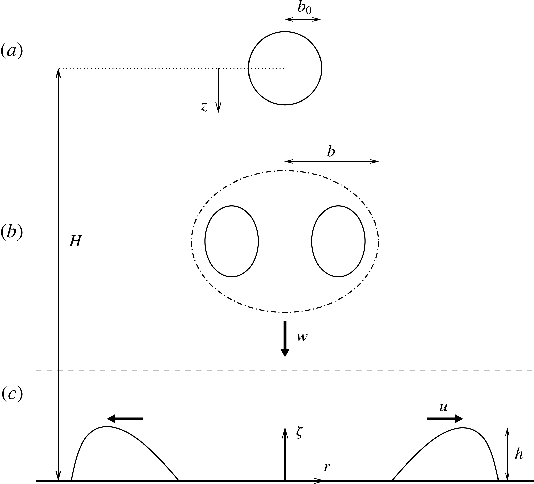
Downdraughts are transient phenomena. When creating idealised models of their behaviour, the two extremes of source condition are either steady or instantaneous. Each of these is worth considering, both because they may prove more tractable and because they provide reference points against which to gauge the range of behaviour. The steady (plume-based) case has already been the subject of a short study by Rooney & Linden (Reference Rooney and Linden2012). Here the case of an impinging thermal is considered. Research into thermals dates back to Scorer (Reference Scorer1957), perhaps even to Thomson & Newall (Reference Thomson and Newall1885). There are useful summaries by Turner (Reference Turner1973) and Morton (Reference Morton and Smith1997). The thermals here are created through a localised perturbation in the initial potential-temperature field of a LES, described fully in later sections. Figure 1 shows a sketch of the initial condition, and subsequent flow regimes of thermal descent and post-impingement spreading.
This study is mainly concerned with the macroscopic features of the flow such as horizontal and vertical length scales, mean flow velocities and the evolution of the temperature perturbation. As well as being interesting in themselves, these are the features that are typically important for parametrisation in numerical weather prediction models, for example.
A sketch of the initial, vertically propagating and horizontally propagating stages of the impinging thermal which is considered here. (a) The initial spherical buoyancy perturbation of radius
 $b_{0}$
centred at an elevation
 $H$
. (b) The descending developed thermal with radial scale
 $b$
and vertical velocity
 $w$
. (c) The radially spreading gravity current with height scale
 $h$
and horizontal velocity
 $u$
. The origin of coordinates (
 $x,y,{\it\zeta}$
) is at the centre of the bottom of the domain. The radial coordinate is
 $r=(x^{2}+y^{2})^{1/2}$
. The downward displacement of the thermal relative to its release point is denoted by
 $z$
.

2. Similarity modelling
The Boussinesq approximation is made in the following analyses.
2.1. Model of the thermal
The initial buoyancy of the thermal is
 $$\begin{eqnarray}B=g_{0}^{\prime }V_{0},\end{eqnarray}$$
where
 $g_{0}^{\prime }$
is the initial reduced gravity and
 $V_{0}$
is the initial volume. In an unstratified ambient,
 $B$
is a conserved quantity. The reduced gravity
 $g^{\prime }$
is conventionally negative for flows with greater density than the ambient; however, flow processes are generally assumed to be the same under buoyancy sign reversal and accompanying reversal of the vertical axis.
Turner (Reference Turner1973, § 6.3.1) discusses the thermal similarity solution, which may be summarised here to give the horizontal radius, velocity and reduced gravity, respectively, in terms of vertical displacement
 $z$
and position
 $\boldsymbol{p}$
relative to the centre of the thermal as
 $$\begin{eqnarray}\displaystyle & \displaystyle b={\it\alpha}z, & \displaystyle\end{eqnarray}$$
 $$\begin{eqnarray}\displaystyle & \displaystyle \displaystyle w_{p}=B^{1/2}z^{-1}f_{1}\left(\frac{\boldsymbol{p}}{b}\right), & \displaystyle\end{eqnarray}$$
 $$\begin{eqnarray}\displaystyle & \displaystyle \displaystyle g_{p}^{\prime }=Bz^{-3}f_{2}\left(\frac{\boldsymbol{p}}{b}\right), & \displaystyle\end{eqnarray}$$
 ${\it\alpha}$
is the entrainment constant. The subscript
 $p$
is added to distinguish terms in this solution set from similar terms used later. This solution is composed of scaling quantities which determine the ‘amplitude’ of the flow variables, and unspecified functions of position (
 $f_{1}$
and
 $f_{2}$
) to describe the interior structure of the flow. The scaling can be derived from dimensional considerations, based on the conserved buoyancy
 $B$
and the use of
 $z$
as a length scale in the absence of any intrinsic length scale of the flow.
The thermal ‘shape factor’
 $m$
is defined as
 $$\begin{eqnarray}m=V/b^{3},\end{eqnarray}$$
where
 $V$
is the volume of the thermal, which increases through entrainment. Experiments by Scorer (Reference Scorer1957) indicate that the oblate spheroid form of the thermal implies a volume–radius relationship such that
 $m\approx 3$
, and
 $m$
is assumed to be approximately constant in a developed thermal.
The experiments of Scorer (Reference Scorer1957) also suggested a mean value of the entrainment constant
 ${\it\alpha}\approx 0.25$
. Turner (Reference Turner1986) quotes the same value for buoyancy-conserving thermals based on later observations. More recently a different experimental technique (Mott & Woods Reference Mott and Woods2011) has produced lower estimates of approximately 0.22–0.24 (where conversion of these results from a volumetric entrainment description to the radial description used here and by Turner (Reference Turner1986) has been performed).
Based on the above, representative vertical velocity and reduced-gravity scales are
 $$\begin{eqnarray}\displaystyle & \displaystyle w={\it\beta}B^{1/2}z^{-1}, & \displaystyle\end{eqnarray}$$
 $$\begin{eqnarray}\displaystyle & \displaystyle g^{\prime }={\it\gamma}Bz^{-3}, & \displaystyle\end{eqnarray}$$
 ${\it\beta}$
and
 ${\it\gamma}$
are as yet unknown coefficients. If we write the thermal buoyancy, Froude number (independent of
 $z$
) and volume, respectively, as
 $$\begin{eqnarray}\displaystyle & \displaystyle B=g^{\prime }V, & \displaystyle\end{eqnarray}$$
 $$\begin{eqnarray}\displaystyle & \displaystyle Fr_{T}=w/(g^{\prime }b)^{1/2}, & \displaystyle\end{eqnarray}$$
 $$\begin{eqnarray}\displaystyle & \displaystyle V=mb^{3}, & \displaystyle\end{eqnarray}$$
 $$\begin{eqnarray}\displaystyle & \displaystyle {\it\beta}=Fr_{T}m^{-1/2}{\it\alpha}^{-1}, & \displaystyle\end{eqnarray}$$
 $$\begin{eqnarray}\displaystyle & \displaystyle {\it\gamma}=m^{-1}{\it\alpha}^{-3}. & \displaystyle\end{eqnarray}$$
 $B$
, vertical coordinate
 $z$
, entrainment constant
 ${\it\alpha}$
, Froude number
 $Fr_{T}$
and shape factor
 $m$
as
 $$\begin{eqnarray}\displaystyle & \displaystyle b={\it\alpha}z, & \displaystyle\end{eqnarray}$$
 $$\begin{eqnarray}\displaystyle & \displaystyle w=(Fr_{T}m^{-1/2}{\it\alpha}^{-1})\,B^{1/2}z^{-1}, & \displaystyle\end{eqnarray}$$
 $$\begin{eqnarray}\displaystyle & \displaystyle g^{\prime }=(m^{-1}{\it\alpha}^{-3})\,Bz^{-3}. & \displaystyle\end{eqnarray}$$
The solution (2.7) has an unphysical origin at
 $z=0$
. In reality, we expect a thermal of this type to begin with some finite radius
 $b_{0}$
, possibly in a state which is not self-similar. (For example, downdraughts may initiate at cloud base with a finite radius and an initial velocity related to the terminal fall speed of hydrometeors.) If the thermal begins with some initial properties such as (2.1), then its subsequent growth may be described in terms of vertical displacement relative to a virtual origin. From (2.7a
), the distance
 $z_{v}$
of the virtual origin from the point of thermal initiation may be estimated as
 $$\begin{eqnarray}z_{v}={\it\alpha}^{-1}b_{0}.\end{eqnarray}$$
We may then re-write the solution (2.7) in terms of
 $z+z_{v}$
rather than
 $z$
. The radial growth then becomes
 $$\begin{eqnarray}b=b_{0}+{\it\alpha}z.\end{eqnarray}$$
Note the implication that the initial conditions of radius, velocity and reduced gravity are not independent for a self-similar thermal. For example the initial reduced gravity is then
 $g_{0}^{\prime }=m^{-1}B\,b_{0}^{-3}$
. Thus, two initial self-similar thermals of identical buoyancy, whose reduced gravities differ by a factor of two, should have radii which differ by a factor of only
 $2^{1/3}\approx 1.26$
. It is expected that transition to self-similarity involves adjustment processes such as entrainment, so that the eventual radius is appropriate to the scale of the reduced gravity.
Finally, the expression for vertical velocity (2.7b
) may be used to relate scales of distance and time. Replacing
 $w$
with
 $\text{d}z/\text{d}t$
and integrating we obtain
 $$\begin{eqnarray}z+z_{v}=\left[2Fr_{T}\,m^{-1/2}{\it\alpha}^{-1}B^{1/2}\,t\right]^{1/2},\end{eqnarray}$$
where
 $t$
is the time from thermal release.
2.2. Model of the axisymmetric gravity current
For the axisymmetric gravity current created by the release of a finite volume of negatively buoyant fluid, Grundy & Rottman (Reference Grundy and Rottman1986) proposed a similarity solution
 $$\begin{eqnarray}\displaystyle & \displaystyle u\propto B^{1/2}r^{-1}, & \displaystyle\end{eqnarray}$$
 $$\begin{eqnarray}\displaystyle & \displaystyle g^{\prime }h\propto B\,r^{-2}, & \displaystyle\end{eqnarray}$$
 $B$
is again the (conserved) buoyancy,
 $r$
is the radial extent of the gravity current,
 $u$
is the horizontal current propagation speed,
 $g^{\prime }$
is a mean or representative reduced gravity and
 $h$
is the height of the gravity current. (2.11) may also be derived by postulating the similarity speed (2.11a
) as a dimensional solution in terms of conserved buoyancy
 $B$
and radius
 $r$
, and also a constant gravity-current Froude number
 $Fr_{C}=u/(g^{\prime }h)^{1/2}$
.
As with the thermal, the buoyancy is related to the volume
 $V$
of the current by
 $B=g^{\prime }V$
. The entrainment behaviour of the current will determine the radial/temporal evolution of
 $V$
, and hence of
 $g^{\prime }$
and
 $h$
. Hallworth et al. (Reference Hallworth, Huppert, Phillips, Sparks and Stephen1996) proposed and verified dimensional arguments that the relative proportion of entrained fluid should be independent of
 $g^{\prime }$
. In experiments in a sector-shaped tank of angle
 $10^{\circ }$
they examined the axisymmetric case and developed a semi-empirical relationship for
 $V/V_{i}$
as a function of
 $r^{3/2}/V_{i}^{1/2}$
, where
 $V_{i}$
is the initial current volume. (The initial volume of Hallworth et al. (Reference Hallworth, Huppert, Phillips, Sparks and Stephen1996) was actually the volume following slumping of a lock-release gravity current; however, in the present configuration no equivalent slumping process occurs during impingement.) This is equivalent to having a functional relationship
 $$\begin{eqnarray}\frac{V}{V_{i}}=f\left(\frac{r}{R_{0}}\right),\end{eqnarray}$$
where
 $R_{0}\sim V_{i}^{1/3}$
is the radial scale of an equivalent quasi-spherical volume of fluid, and
 $f$
is an unknown function of the dimensionless radius.
Based on these considerations, (2.11) may then be written
 $$\begin{eqnarray}\displaystyle & \displaystyle u=Fr_{C}\,{\it\lambda}^{1/2}B^{1/2}r^{-1}, & \displaystyle\end{eqnarray}$$
 $$\begin{eqnarray}\displaystyle & \displaystyle g^{\prime }=B\left[V_{i}\,f\left(\frac{r}{R_{0}}\right)\right]^{-1}, & \displaystyle\end{eqnarray}$$
 $$\begin{eqnarray}\displaystyle & \displaystyle h={\it\lambda}r^{-2}V_{i}\,f\left(\frac{r}{R_{0}}\right), & \displaystyle\end{eqnarray}$$
 ${\it\lambda}$
is a constant with a value suggested by Hallworth et al. (Reference Hallworth, Huppert, Phillips, Sparks and Stephen1996) of
 ${\rm\pi}^{-1}$
.
2.3. Combining the solutions
To combine the thermal and gravity-current solutions, we make the assumption that the gravity-current buoyancy and initial volume are those of the thermal at impingement. This neglects any transitional processes in the impingement region, but as a first approximation it should indicate how the current arising from thermal impingement may behave. The observed behaviour in the impingement region will be discussed in § 4.
Thus, if the thermal originates at some height
 $H$
above the impact point, the volume at impingement is
 $$\begin{eqnarray}V_{i}=mb^{3}=m\,{\it\alpha}^{3}H^{3}\left(1+\frac{b_{0}}{{\it\alpha}H}\right)^{3},\end{eqnarray}$$
from (2.3) and (2.9). Matching the solutions involves keeping the same value of
 $B$
throughout, and also substituting for
 $V_{i}$
, hence, from (2.13) and (2.14) we have the combined solution
 $$\begin{eqnarray}\displaystyle & \displaystyle u=Fr_{C}\,{\it\lambda}^{1/2}B^{1/2}r^{-1}, & \displaystyle\end{eqnarray}$$
 $$\begin{eqnarray}\displaystyle & \displaystyle g^{\prime }=m^{-1}{\it\alpha}^{-3}BH^{-3}\left(1+\frac{b_{0}}{{\it\alpha}H}\right)^{-3}f^{-1}, & \displaystyle\end{eqnarray}$$
 $$\begin{eqnarray}\displaystyle & \displaystyle \displaystyle \frac{h}{H}={\it\lambda}\,m\,{\it\alpha}^{3}\left(1+\frac{b_{0}}{{\it\alpha}H}\right)^{3}\left(\frac{r}{H}\right)^{-2}f. & \displaystyle\end{eqnarray}$$
 $V$
.
As with the thermal, we may make the substitution
 $u=\text{d}r/\text{d}t$
and integrate to obtain the radial position as a function of time after impingement,
 $$\begin{eqnarray}r^{2}-R_{0}^{2}=2Fr_{C}{\it\lambda}^{1/2}\,B^{1/2}\,(t-t_{i}),\end{eqnarray}$$
where
 $t_{i}$
is the time at which the thermal impinges on the ground, and
 $R_{0}$
is again the radial scale of the current prior to spreading. From (2.10), the time scale
 $t_{i}$
is
 $$\begin{eqnarray}t_{i}=\frac{m^{1/2}{\it\alpha}}{2Fr_{T}}\,B^{-1/2}\,H^{2}\,\left(1+\frac{b_{0}}{{\it\alpha}H}\right)^{2}.\end{eqnarray}$$
Thus far, the source length scale
 $R_{0}$
has only appeared as an integration constant in the radial propagation (2.16). It is evident that for
 $r\gg R_{0}$
this length scale becomes unimportant, and the radial spread may be approximated as
 $$\begin{eqnarray}r=(2Fr_{C})^{1/2}{\it\lambda}^{1/4}\,B^{1/4}\,(t-t_{i})^{1/2}.\end{eqnarray}$$
In their experiments on microburst modelling, Lundgren et al. (Reference Lundgren, Yao and Mansour1992) took the source length scale
 $R_{0}$
to be the equivalent spherical radius of the impinging thermal, and formed a time scale
 $t_{0}$
based on
 $R_{0}$
and the reduced gravity close to impingement
 $g_{i}^{\prime }$
, namely
 $t_{0}=(R_{0}/g_{i}^{\prime })^{1/2}$
. They found that using these scales, their non-dimensionalised data on radial spread versus time collapsed well onto a single trajectory. In this context, the particular form of (2.18) becomes interesting, since dividing it by
 $R_{0}$
yields
 $$\begin{eqnarray}\frac{r}{R_{0}}=(2Fr_{C})^{1/2}{\it\lambda}^{1/4}\left(\frac{t-t_{i}}{R_{0}^{2}\,B^{-1/2}}\right)^{1/2}.\end{eqnarray}$$
Now from (2.13b
) and the specification of
 $R_{0}$
as the equivalent ‘spherical’ scale of the impinging thermal, we have
 $B\sim g_{i}^{\prime }R_{0}^{3}$
, and hence
 $R_{0}^{2}B^{-1/2}\sim (R_{0}/g_{i}^{\prime })^{1/2}=t_{0}$
. Thus, while the similarity-based result (2.18) does not depend on
 $R_{0}$
, this solution can be used to predict the scaling which unified the results of Lundgren et al. (Reference Lundgren, Yao and Mansour1992).
For thermals which descend a significant distance, it useful to obtain
 $R_{0}$
from more fundamental parameters. From (2.14),
 $$\begin{eqnarray}R_{0}=\left(\frac{3m}{4{\rm\pi}}\right)^{1/3}(b_{0}+{\it\alpha}H),\end{eqnarray}$$
which for
 $m=3$
is approximately 90 % of the predicted horizontal scale of the thermal.
Returning to (2.15), there is one limiting case to consider, when the parameter
 $b_{0}/{\it\alpha}H$
is very small (the theoretical upper bound of
 $b_{0}/{\it\alpha}H$
being approximately
 ${\it\alpha}^{-1}$
). This corresponds to a thermal which travels a significant distance before impinging, such that its final radius is much greater than its initial radius. In this case (2.15) may be approximated by
 $$\begin{eqnarray}\displaystyle & \displaystyle u=Fr_{C}\,{\it\lambda}^{1/2}B^{1/2}r^{-1}, & \displaystyle\end{eqnarray}$$
 $$\begin{eqnarray}\displaystyle & \displaystyle g^{\prime }=m^{-1}{\it\alpha}^{-3}BH^{-3}f^{-1}, & \displaystyle\end{eqnarray}$$
 $$\begin{eqnarray}\displaystyle & \displaystyle \frac{h}{H}={\it\lambda}\,m\,{\it\alpha}^{3}\displaystyle \left(\frac{r}{H}\right)^{-2}f. & \displaystyle\end{eqnarray}$$
3. Large-eddy modelling
Numerical experiments using LES have been carried out to compare with the above analysis.
3.1. Model description
LES is a technique for numerical solution of the time-dependent Navier–Stokes equations, in which flow features are resolved to a scale comparable to that of the numerical grid, with an additional subgrid model for the unresolved part of the flow. The technique has been reviewed by Mason (Reference Mason1994). The large-eddy model (LEM) used here has a history of use and development at the Met Office and has been described by Mason (Reference Mason1989) and Brown, Derbyshire & Mason (Reference Brown, Derbyshire and Mason1994), and documented by Gray et al. (Reference Gray, Petch, Derbyshire, Brown, Lock, Swann and Brown2001). The subgrid component of this model uses a Smagorinsky representation of subgrid stress, with a mixing length which relaxes to
 $kz_{0}$
at the surface (where
 $z_{0}$
is the roughness length and
 $k\approx 0.4$
is von Karman’s constant). It has been used extensively for atmospheric boundary-layer and cloud studies, and recently also for the simulation of idealised plume flow (Devenish, Rooney & Thomson Reference Devenish, Rooney and Thomson2010, which also contains a summary of the numerical procedure). In the results presented here, the Smagorinsky coefficient which relates the subgrid eddy-viscosity length scale to the model gridscale was set to 0.1.
The domain of the numerical experiments consisted of
 $512\times 512$
gridpoints in the horizontal and 241 gridpoints in the vertical, with a grid resolution of 50 m in all directions. This produces a domain of height 12 km, and length and width 25.55 km, or just over double the height. The resolution is comparable to that of similar simulations of downbursts or thermals (Bryan & Fritsch Reference Bryan and Fritsch2002; Anabor et al.
Reference Anabor, Rizza, Nascimento and Degrazia2011). The domain was periodic in both horizontal directions, with free-slip and no-slip boundary conditions on the top and bottom, respectively.
The model configuration uses the Boussinesq formulation of the equations and has an implementation of subgrid backscatter of turbulent kinetic energy from small to large scales. This has been shown to improve the representation of sheared flows and stratified flow regions (Brown et al.
Reference Brown, Derbyshire and Mason1994). The roughness length for momentum
 $z_{0}$
was set to
 $2.0\times 10^{-4}$
m, as was the roughness length for scalar transport. The surface temperature was set to the same value as the initial background potential temperature (300 K) and surface heat flux was suppressed to provide a boundary condition which conserves buoyancy. The model was run without interaction of a humidity field (so-called ‘dry’ mode).
Limited testing showed that the model performance was not greatly sensitive to the choice of Smagorinsky coefficient or surface roughness length. For instance, the level of agreement with the similarity framework was not affected, but the values of the proportionality constants could vary to some degree. However, without the backscatter scheme the model was found to be more dissipative of the gravity-current outflow. The results obtained with the backscatter scheme were similar to those produced when running as an ‘implicit’ LES, that is, allowing numerical dissipation within the model to act in place of an explicit subgrid model.
3.2. Initial configuration, run length and output
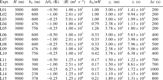
The experiments consisted of the initialisation of a cold parcel of fluid in an otherwise homogeneous field, which was then allowed to evolve freely. The lower boundary of the domain represents an impermeable solid surface, upon which the descending thermal impinges. The range of experiments, and the important parameters of each, are listed in table 1.
Each simulation was initialised with a ‘cold bubble’ of radius
 $b_{0}$
centred at a height
 $H$
above the surface, see figure 1. The bubble is merely a temperature perturbation in the otherwise homogeneous fluid, the term does not indicate a region of different phase. It has a maximum (negative) potential-temperature difference
 ${\rm\Delta}{\it\theta}_{0}$
from the surrounding environment which is at a uniform potential temperature
 ${\it\theta}_{a}=300$
K.
The bubble was initialised in two stages. In the first stage, the distribution of the perturbation in its interior was set according to
 $$\begin{eqnarray}{\rm\Delta}{\it\theta}=\left\{\begin{array}{@{}ll@{}}{\rm\Delta}{\it\theta}_{0}, & {\it\rho}\leqslant (1-{\it\phi}),\\ {\rm\Delta}{\it\theta}_{0}\cos ^{2}\left[\displaystyle \frac{{\rm\pi}}{2}\frac{{\it\rho}-(1-{\it\phi})}{{\it\phi}}\right], & (1-{\it\phi})<{\it\rho}\leqslant 1,\end{array}\right.\end{eqnarray}$$
where
 $b_{0}{\it\rho}$
is the distance from the bubble centre and
 ${\it\phi}$
 $({<}1)$
determines the extent of an ‘edge’ region where the potential temperature is blended smoothly between the interior and ambient values. In the simulations presented here,
 ${\it\phi}=0.25$
. The total buoyancy of the bubble is obtained by integrating the potential-temperature distribution (3.1) over its volume. This yields
 $$\begin{eqnarray}B\approx 0.678\,g\frac{{\rm\Delta}{\it\theta}_{0}}{{\it\theta}_{a}}\,\frac{4}{3}{\rm\pi}b_{0}^{3}\approx 2.84\,g_{0}^{\prime }\,b_{0}^{3},\end{eqnarray}$$
where
 $g_{0}^{\prime }=g{\rm\Delta}{\it\theta}_{0}/{\it\theta}_{a}$
. Comparing (3.2) with the thermal relationship (2.5a
) implies an equivalent value of the shape factor of
 $m\approx 2.84$
. This is similar to that estimated for a developed thermal of the same (horizontal) radius.
In the second stage of initialisation, randomly selected pairs of points within the bubble interior had their temperature perturbations swapped. This had the effect of distributing some of the reduced-buoyancy points from the bubble edge into the centre of the bubble, and vice versa. It was found that this randomisation of the perturbation broke down the flow symmetry, and was particularly necessary in the implicit LES testing.
Three sets of five experiments were carried out. Each set of five is based on three different initial radii and temperature perturbations, such that three of the five have the same initial radius and three have the same initial buoyancy. Variation across sets comes through the choice of two different release heights and ‘baseline’ radii. The parameter combinations span approximately one order of magnitude of the source-size parameter,
 $0.13\leqslant b_{0}/{\it\alpha}H\leqslant 1.26$
, and approximately one-and-a-half orders of magnitude of thermal buoyancy,
 $6.27\times 10^{5}~\text{m}^{4}~\text{s}^{-2}\leqslant B\leqslant 2.01\times 10^{7}~\text{m}^{4}~\text{s}^{-2}$
.
Some of the heights and radii are of comparable magnitude to the downdraught dimensions observed by Giangrande et al. (Reference Giangrande, Collis, Straka, Protat, Williams and Krueger2013). However, the analytical approach taken here is ultimately to describe the flow features in a dimensionless framework. The assumption underlying this is that these structures are similar across a range of dimensions, provided the Reynolds number is sufficiently large. The agreement of dimensionless results between experiments with different magnitudes of initial radius, to be shown later, also constitutes a demonstration of model convergence. That is, doubling the initial radius is, in terms of the flow numerics, equivalent to keeping the radius fixed but increasing the grid resolution by the same factor. An effort has also been made to minimise the effects of finite domain size, by specifying a wide domain with a top which is significantly above the higher of the two release heights.
As can be seen from table 1, the different buoyancies and release heights give rise to a large range of estimated impingement time scales,
 $t_{i}$
. The model runs produced output dumps at 23 regular intervals, with the time interval between dumps
 ${\rm\Delta}t$
adjusted for each experiment to ensure the run (of length
 $23{\rm\Delta}t$
) encompassed the thermal descent as well as some degree of spread on the domain floor. Generally, the experiments were designed to terminate when the gravity-current spread was around 5 km in radius, at which point the current front enclosed a relatively small area of the domain floor. If the flows are allowed to continue to propagate close to the boundaries of the domain, the effect of the periodic boundary conditions eventually begins to restrict the flow development.
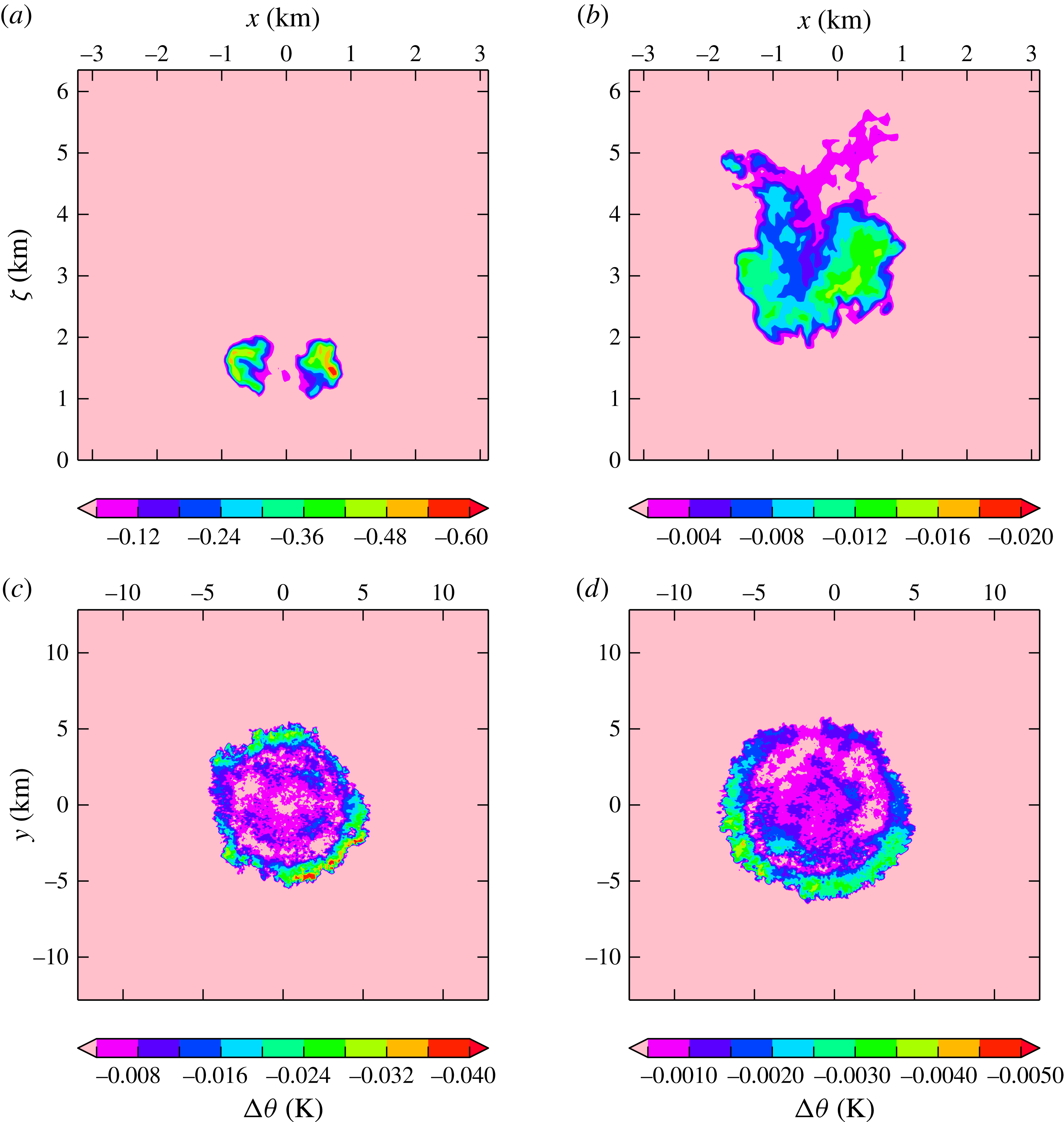
The model adjusts the time interval based on its internal selection of time step against convergence criteria, hence the dumps are approximately rather than exactly spaced at the intervals listed in table 1. Examples of sections through the potential-temperature perturbation fields of some dumps are shown in figure 2.
Sections through the simulation domain for experiments L04 (a,c) and L12 (b,d), see table 1. The domain size for all experiments was approximately
 $25\times 25~\text{km}^{2}$
in the horizontal and 12 km in the vertical. The colours show negative potential-temperature perturbations
 ${\rm\Delta}{\it\theta}$
(K) from the background value. Contour levels have different magnitudes on each plot, but the same colour scale to focus on comparison of the flow features. (a) L04, vertical section through the lower central portion of the domain, approximately 604 s into the simulation. (b) L12, Vertical section through the lower central portion of the domain, approximately 4908 s into the simulation. (c) L04, horizontal section through the domain at height 200 m, approximately 4617 s into the simulation. (d) L12, horizontal section through the domain at height 200 m, approximately 16 108 s into the simulation.

Details of the LES experiments. Two release heights (
 $H$
) and two radius ranges (
 $b_{0}$
) have been chosen. At each height, parameter variation around a `central' initial radius and potential-temperature perturbation (
 ${\rm\Delta}{\it\theta}_{0}$
) produces five experiments, of which three have the same initial radius and three have the same buoyancy (
 $B$
). Note that
 ${\rm\Delta}{\it\theta}_{0}$
, and consequently
 $B$
, is negative; however,
 $B$
is replaced by its modulus in the analysis of the data. The combinations of height and initial radius have been chosen to produce different magnitudes of the parameter
 $b_{0}/{\it\alpha}H$
. The virtual origin is estimated as
 $z_{v}={\it\alpha}^{-1}b_{0}$
. The time to impingement
 $t_{i}$
is calculated using (2.17). The values shown have been calculated assuming
 ${\it\alpha}=0.2$
,
 $m=3$
and
 $Fr_{T}=1.4$
.
 ${\rm\Delta}t$
refers to the (approximate) model time interval between dumps, each model run was of approximate length
 $23{\rm\Delta}t$
. Animations of experiments L03, L08 and L13 have been provided as supplementary material.

3.3. Tracking of buoyant fluid
For each model dump, the largest (negative) potential-temperature perturbation,
 ${\rm\Delta}{\it\theta}_{\mathit{max}}$
in the domain was first found. The maximum reduced gravity is calculated from the maximum potential temperature to be
 $$\begin{eqnarray}g_{\mathit{max}}^{\prime }=g{\rm\Delta}{\it\theta}_{\mathit{max}}/{\it\theta}_{a}.\end{eqnarray}$$
To simplify the analysis, both
 $g^{\prime }$
and
 $B$
of the negatively buoyant fluid are replaced by their moduli from here on.
Locations of buoyant fluid were identified as those points whose potential-temperature perturbation
 ${\rm\Delta}{\it\theta}$
satisfied
 $$\begin{eqnarray}|{\rm\Delta}{\it\theta}-{\rm\Delta}{\it\theta}_{\mathit{max}}|<{\it\epsilon}\,|{\rm\Delta}{\it\theta}_{\mathit{max}}|.\end{eqnarray}$$
The buoyancy threshold
 ${\it\epsilon}$
may take values between 0 and 1, and the higher the value of
 ${\it\epsilon}$
, the more points are identified. A value of
 ${\it\epsilon}=0.8$
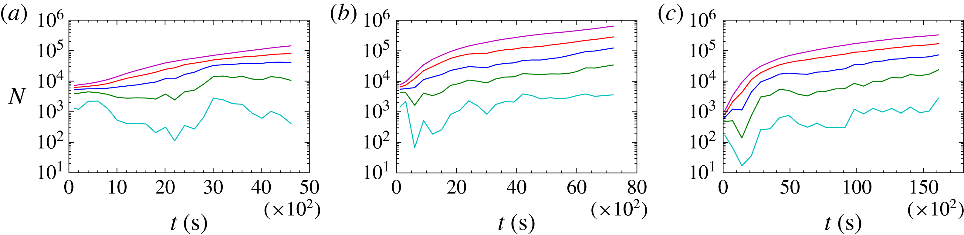
, which identifies points whose perturbation is 20 % or more of the largest in that dump, has been used to generate most of the results which will be shown. The choice of threshold is a balance between identifying the dynamically active part of the flow, and seeking to describe how the major part of the buoyant fluid is dispersed. The former is a concern for numerical experiments, where numerical diffusion may unphysically increase the spread of the temperature perturbation at low limits. The latter is important when considering comparisons, for example, with laboratory experiments in which visual or optical methods are used for tracking buoyant fluid which has been marked with dye. To illustrate, the numbers of gridpoints identified by a range of thresholds are shown in the examples in figure 3. (Later, figure 8 will give an example of the degree of sensitivity of the model results to the choice of threshold.) The value of
 ${\it\epsilon}=0.8$
is taken to be optimal in these circumstances.
The location data, with origin at the centre of the domain floor, were then processed to provide macroscopic measures of the flow field. Vertical coordinates (
 ${\it\zeta}$
, measured from the bottom of the domain) were combined to yield the mean and maximum,
 $\bar{{\it\zeta}}$
and
 ${\it\zeta}_{\mathit{max}}$
respectively. The downward vertical displacement of a thermal from its release point is then taken to be
 $z=H-\bar{{\it\zeta}}$
.
For the horizontal coordinates (
 $x,y$
) the position of the ‘centre of mass’ of buoyant fluid (
 $\bar{x},\bar{y}$
) was obtained simply by averaging the coordinate set. The horizontal (radial) distances of each point from the origin and from the centre of mass,
 $r$
and
 $r^{\prime }$
respectively, were then calculated as
 $$\begin{eqnarray}\displaystyle r & = & \displaystyle \left(x^{2}+y^{2}\right)^{1/2},\end{eqnarray}$$
 $$\begin{eqnarray}\displaystyle r^{\prime } & = & \displaystyle \left((x-\bar{x})^{2}+(y-\bar{y})^{2}\right)^{1/2}.\end{eqnarray}$$
 $r_{\mathit{max}}$
and
 $r_{\mathit{max}}^{\prime }$
at each dump time were obtained.
Throughout each experiment, an integral, or top-hat, scale may be derived for the vertical extent of the buoyant region. This was obtained by first identifying the position of
 ${\rm\Delta}{\it\theta}_{\mathit{max}}$
in each dump. A vertical column from the domain, centred horizontally on this position, was then averaged horizontally to give a vertical profile,
 $\overline{{\rm\Delta}{\it\theta}}({\it\zeta})$
. The column extended five gridpoints in the
 $x$
and
 $y$
directions, so that the average at each height was over a square grid of 25 values, with the position of the maximum perturbation at the centre. The averaging had the effect of producing a slightly smoothed profile, and it was found that the integral-scale results were very similar with a column of nine gridpoints in each direction.
To calculate an integral scale
 ${\it\zeta}_{I}$
, the profile was then integrated vertically and divided by the maximum perturbation,
 $$\begin{eqnarray}{\it\zeta}_{I}=\frac{1}{{\rm\Delta}{\it\theta}_{\mathit{max}}}\mathop{\sum }_{{\rm\Delta}{\it\theta}<0}\;\overline{{\rm\Delta}{\it\theta}}\,{\rm\Delta}{\it\zeta},\end{eqnarray}$$
where
 ${\rm\Delta}{\it\zeta}$
is the vertical grid spacing. The summation (3.6) receives only a small contribution from any diffuse regions of marginal buoyancy, and hence is more likely to yield a vertical scale for the dynamically significant part of the flow.
The number of gridpoints falling within different buoyancy thresholds, demonstrated using three example experiments. Each line connects the number of points
 $N$
in the model dumps (created at different experiment times
 $t$
) whose potential-temperature perturbation satisfies the criterion (3.4), for different values of
 ${\it\epsilon}$
as follows: cyan,
 ${\it\epsilon}=0.2$
; green,
 ${\it\epsilon}=0.4$
; blue,
 ${\it\epsilon}=0.6$
; red,
 ${\it\epsilon}=0.8$
; magenta,
 ${\it\epsilon}=0.95$
. Note that the value of the maximum potential-temperature perturbation
 ${\rm\Delta}{\it\theta}_{\mathit{max}}$
is identified within each dump, and varies from one dump to the next. Most of the subsequent results are based on points identified using a threshold value of
 ${\it\epsilon}=0.8$
: (a) L03; (b) L07; (c) L11.

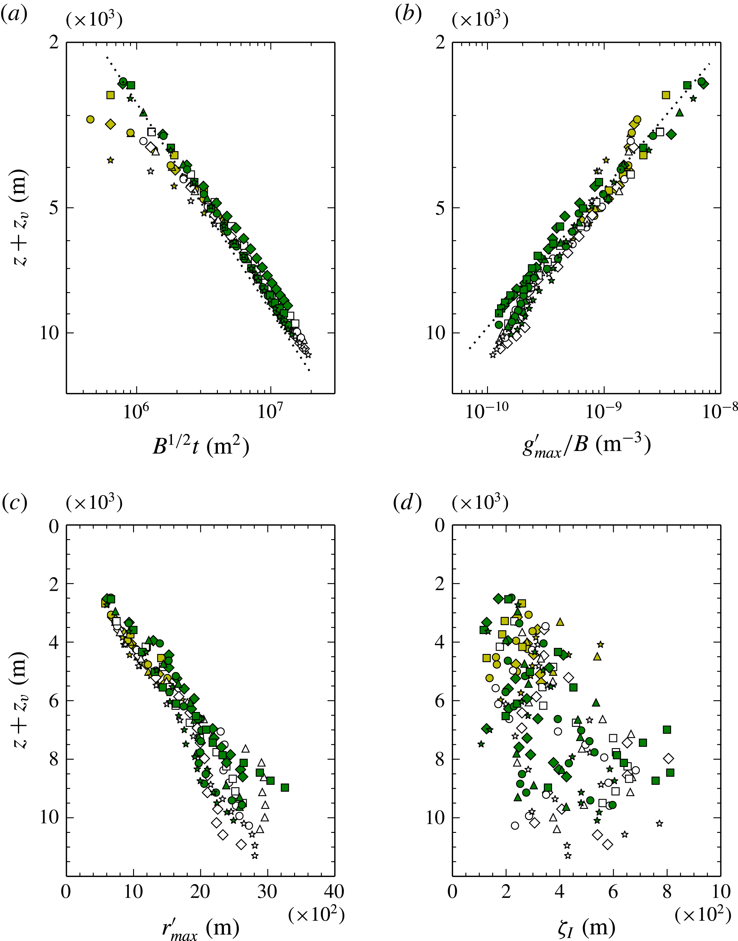
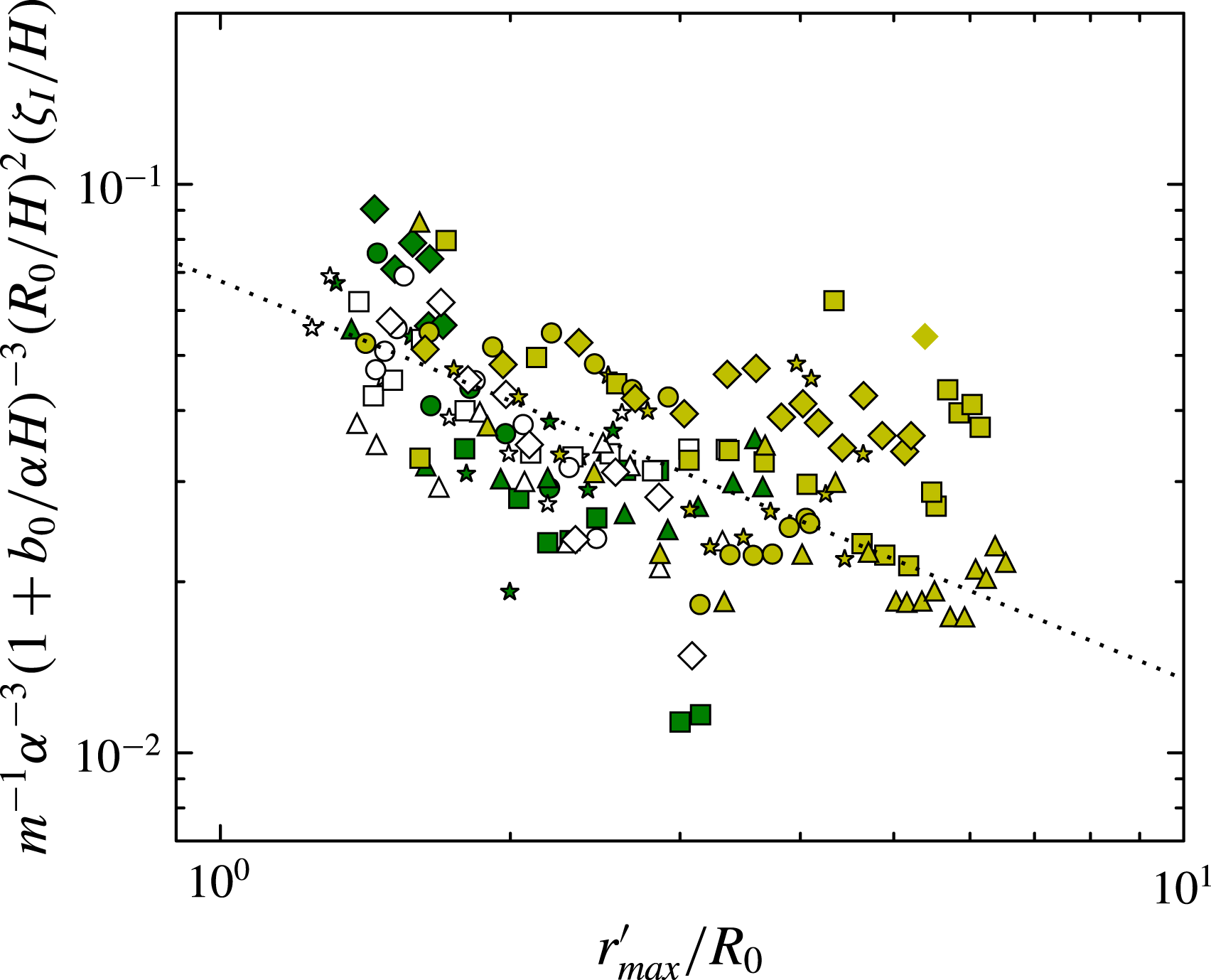
Flow characteristics through the descent phase. In all cases the vertical axis shows downward vertical displacement
 $z$
from the release heights of the negatively buoyant thermals, with a correction
 $z_{v}$
for the virtual origin. The symbols are coloured by simulation set, yellow: L01–L05, white: L06–L10, green: L11–L15, with the symbol ordering (diamond, triangle, circle, square, star) within each set. The data are shown for dump times prior to the estimated impingement time
 $t_{i}$
, see table 1. (a) The scaled time from release
 $B^{1/2}t$
. The dotted line shows
 $z+z_{v}=2.8(B^{1/2}t)^{1/2}$
. (b) The scaled maximum (modulus) reduced gravity
 $g_{\mathit{max}}^{\prime }/B$
. The dotted line shows
 $z+z_{v}=4.5(g_{\mathit{max}}^{\prime }/B)^{-1/3}$
. (c) The maximum radius of the negatively buoyant fluid relative to its centre of mass. (d) The vertical integral scale of the negatively buoyant fluid.

4. Model results and analysis
4.1. Thermal descent
The vertical thermal displacement
 $z$
, corrected to include a virtual origin correction
 $z_{v}$
, is plotted for all experiments and dump times in figure 4(a). The scaling of time
 $t$
by
 $B^{1/2}$
in this plot is effective at collapsing a range of descent rates in these experiments, in which the run lengths varied between approximately 4600 and 23 000 s.
The value of
 $z_{v}$
for each experiment is obtained from (2.8) with the same value of
 ${\it\alpha}$
for all cases, see below and also table 1. While the experiments presented here are initialised with a stationary, spherical cold bubble rather than a fully developed self-similar thermal, the simple theoretical expression (2.8) performs satisfactorily as an estimator of
 $z_{v}$
. The degree of collapse of all the data onto a single line was found to depend weakly on
 ${\it\alpha}$
, and figure 4(a) has been generated using
 ${\it\alpha}=0.2$
. This is similar in magnitude to other estimates discussed in § 2.1.
The line drawn on the plot is based on (2.10) and has equation
 $z+z_{v}=2.8(B^{1/2}t)^{1/2}$
. Comparing this fit with (2.10) and taking
 $m\approx 3$
and
 ${\it\alpha}=0.2$
yields a representative value of the Froude number for all experiments of
 $Fr_{T}\approx 1.4$
. A Froude number of order unity is typical for buoyancy-driven flows.
Figure 4(b) shows the evolution of maximum reduced gravity
 $g_{\mathit{max}}^{\prime }$
. Again, scaling by
 $B$
according to (2.7c
) produces a good collapse of the data. The data fall approximately on the line
 $z+z_{v}=4.5(g_{\mathit{max}}^{\prime }/B)^{-1/3}$
, hence taking
 $m\approx 3$
and
 ${\it\alpha}=0.2$
implies a relationship between the reduced-gravity scale and the maximum observed reduced gravity of the descending thermal of
 $g_{\mathit{max}}^{\prime }\approx 2.2\,g^{\prime }$
, from (2.7c
).
Figures 4(c,d) show data relating to the horizontal and vertical extent of the buoyant fluid, namely the maximum horizontal radius from the centre of mass,
 $r_{\mathit{max}}^{\prime }$
, and vertical integral scale,
 ${\it\zeta}_{I}$
. It appears that the thermal shape reflected by these metrics is subject to more variation than its rates of descent and buoyancy reduction. The explanation of this variation is that the buoyant fluid is not distributed with enough uniformity within the vortical structure of the descending thermals to achieve a state of steadiness within bounds of self-similarity. This is consistent with evidence from flow snapshots, e.g. figure 2. It is possible that a longer drop length would eventually provide sufficient time for mixing and diffusion to achieve a thermal with self-similar buoyant structure. However, figure 4(a) shows that, despite this variability in the internal thermal structure, the large-scale dynamics are well described using only the total buoyancy of the flow.
4.2. Impingement region
The onset of the spreading gravity-current phase of the flow may be defined in various ways. Here, the transition from descending to spreading flow is taken to be the predicted impingement time scale
 $t_{i}$
from (2.17), using values of
 ${\it\alpha}=0.2$
and
 $Fr_{T}=1.4$
obtained in the previous subsection. The resulting times are presented in table 1.
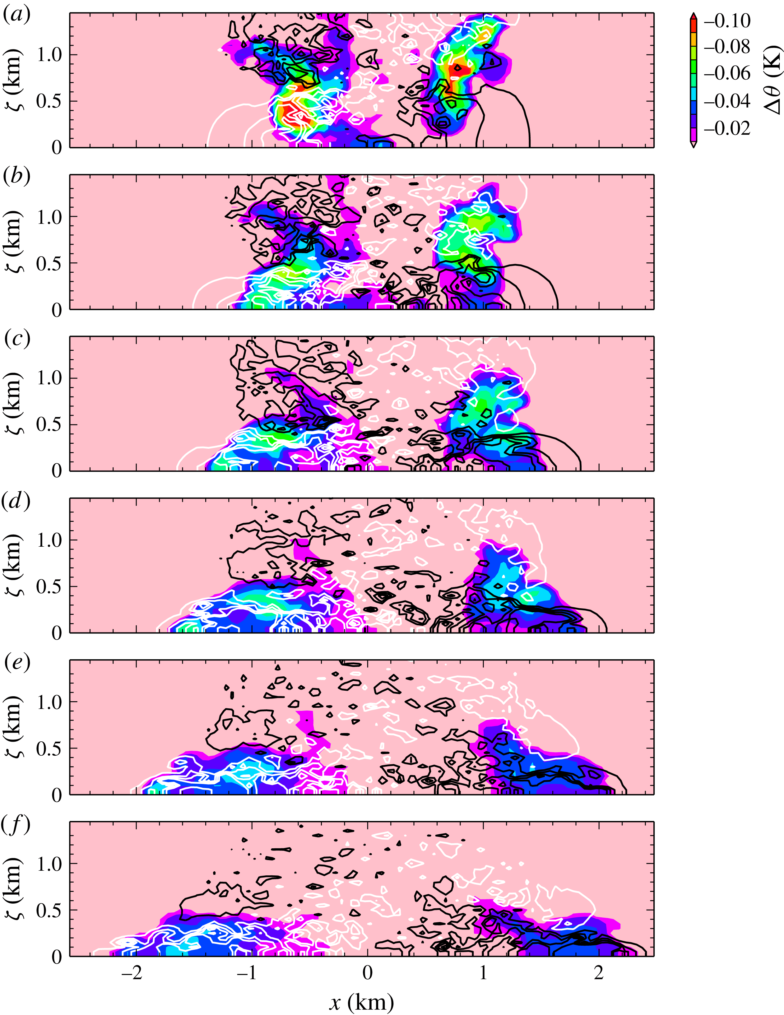
Figure 5 shows an example of thermal impingement taken from one simulation, which highlights several relevant features (see also the flow animations uploaded as supplementary material available at http://dx.doi.org/10.1017/jfm.2015.484). The flow has a small-scale structure indicating some level of turbulence. The horizontal-velocity contours in the upper frames nonetheless show a large-scale quadrupole structure in cross-section, indicative of the vortex ring-like circulation generated by the thermal and imposed on the small-scale flow. The impingement phase of the thermal does not exhibit any obvious near-surface vorticity generation, such as has been observed in laminar flows (Walker et al. Reference Walker, Smith, Cerra and Doligalski1987), and this may be due to turbulent disruption of the surface layer. However, in the last frame it can be seen that a region of recirculation has developed above and just behind the head of the expanding gravity current, indicated by the velocity contour of inward-pointing sign.
Vertical sections through the simulation domain for experiment L03, see table 1. The panels show model data from consecutive dumps at approximately 200 s intervals, in descending order, starting at 1802 s and finishing at 2800 s. The view is restricted to the lower, central portion of the domain containing the thermal impingement zone. The colours show negative potential-temperature perturbations
 ${\rm\Delta}{\it\theta}$
(K) from the background value. The lines show contours of the horizontal-velocity component in the
 $x$
-direction. Black lines show positive (rightward) speeds of 0.5, 1.0, 1.5 and 2.0 m
 $\text{s}^{-1}$
and white lines show negative (leftward) speeds of
 $-0.5$
,
 $-1.0$
,
 $-1.5$
and
 $-2.0$
m
 $\text{s}^{-1}$
. Adjacent black and white contours are of the lowest magnitudes.

One notable feature in the evolution of the gravity current is the contrast between the ‘vertical’ and ‘horizontal’ faces of the flow. As the gravity current evolves, the velocity contours at the leading edge tighten up and couple to the spreading front of buoyant fluid. This is an example of frontogenesis (Linden Reference Linden, Chassignet, Cenedese and Verron2012). On the upper surface of the current, however, shear and vorticity generation act to broaden the interface region in the vertical direction, and it is also possible that numerical effects may increase, or alter the characteristics of, this mixing.
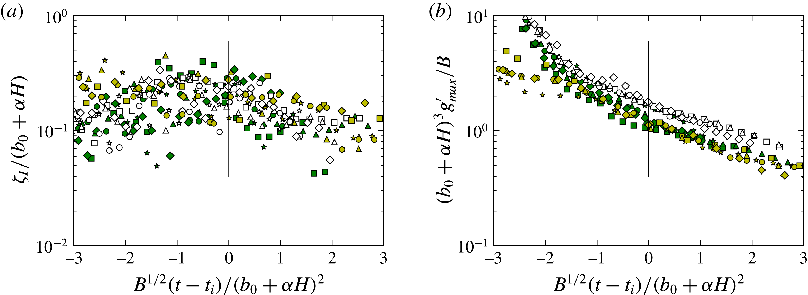
Figure 6 shows the transition of the depth scale and reduced gravity of the buoyant fluid through the impingement region. These have been plotted against time relative to
 $t_{i}$
, and all quantities have been non-dimensionalised by the buoyancy
 $B$
and the theoretical thermal radius at impingement
 $(b_{0}+{\it\alpha}H)$
. The non-dimensional time
 $B^{1/2}(t-t_{i})/(b_{0}+{\it\alpha}H)^{2}$
ranges from
 $-3$
to 3 in these figures, and the interval between
 $-3$
and 0 is almost the entirety of the descent phase for all experiments, see (2.17).
The plots show that the evolution is quite smooth. The depth, which has been increasing through the thermal descent, levels off as
 $t$
approaches
 $t_{i}$
, before starting to decrease in the gravity-current phase. The reduced gravity decreases throughout, but does not exhibit any sudden change in gradient around
 $t=t_{i}$
. Figure 6(b) shows that in fact the least smooth section of the
 $g_{\mathit{max}}^{\prime }$
evolution is during the first half of the descent phase, after the cold bubble is released from rest. This may indicate that the major flow adjustment is associated with the post-release phase rather than impingement, and that the thermal reaches the transition zone in a ‘spun-up’ state. It can therefore perhaps evolve more smoothly, and attain self-similarity more quickly, than the traditional lock-release gravity current (Rottman & Simpson Reference Rottman and Simpson1983).
The evolution of (a) the integral depth scale
 ${\it\zeta}_{I}$
and (b) the maximum reduced gravity
 $g_{\mathit{max}}^{\prime }$
, as the flow makes the transition from thermal to gravity current. The data are plotted against time relative to the predicted impingement time
 $t_{i}$
, and all quantities have been non-dimensionalised using the buoyancy
 $B$
and the predicted radius at impingement
 $(b_{0}+{\it\alpha}H)$
. The vertical lines mark the point
 $t=t_{i}$
, and the left-hand side of the figure covers the majority of the thermal-descent phase.

4.3. Speed of radial spread
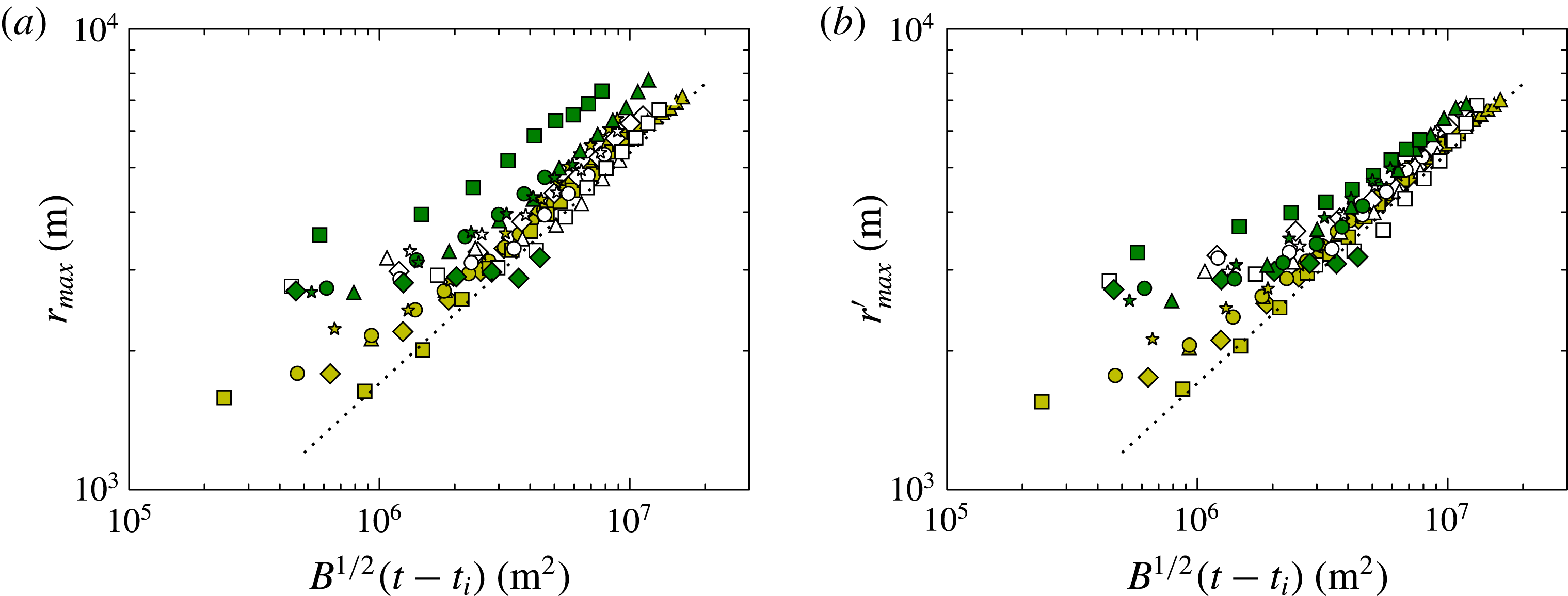
Spread of the radial gravity current arising from thermal impingement. Data are identified as in figure 4. The dotted line with equation
 $r_{\mathit{max}}^{\prime }=1.7B^{1/4}(t-t_{i})^{1/2}$
is the same in both plots. (a) Maximum radial extent of buoyant fluid relative to the centre of the domain, plotted against scaled time since the predicted thermal impingement. (b) Maximum radial extent of buoyant fluid relative to the centre of mass of the fluid, plotted against scaled time since the predicted thermal impingement. This reference frame makes allowance for off-centre drift in the descending thermal.

The maximum-radius data are compared with the similarity prediction (2.18) in figures 7(a,b). The data tend to the similarity power law at larger radii for both calculation methods. However, the maximum radius relative to the centre of mass,
 $r_{\mathit{max}}^{\prime }$
, is better at grouping the data along a single line. This indicates that it is important to account for sideways drift in thermal descent. The numerical experiments were initiated with a still environment, so the observed drift must arise from unsteadiness or asymmetry in the thermal flow.
The data in figure 7(b) tend to the line
 $r_{\mathit{max}}^{\prime }=1.7B^{1/4}(t-t_{i})^{1/2}$
, shown. Comparing with (2.18) and taking
 ${\it\lambda}={\rm\pi}^{-1}$
would yield a value of the gravity-current Froude number of
 $Fr_{C}\approx 2.9$
, which is larger than expected. Alternatively, assuming that
 $Fr_{C}$
should have a more typical value such as 1.4 (Linden Reference Linden, Chassignet, Cenedese and Verron2012) implies a value of
 ${\it\lambda}\approx 1$
. A value of
 ${\it\lambda}=1$
will therefore be assumed from now on.
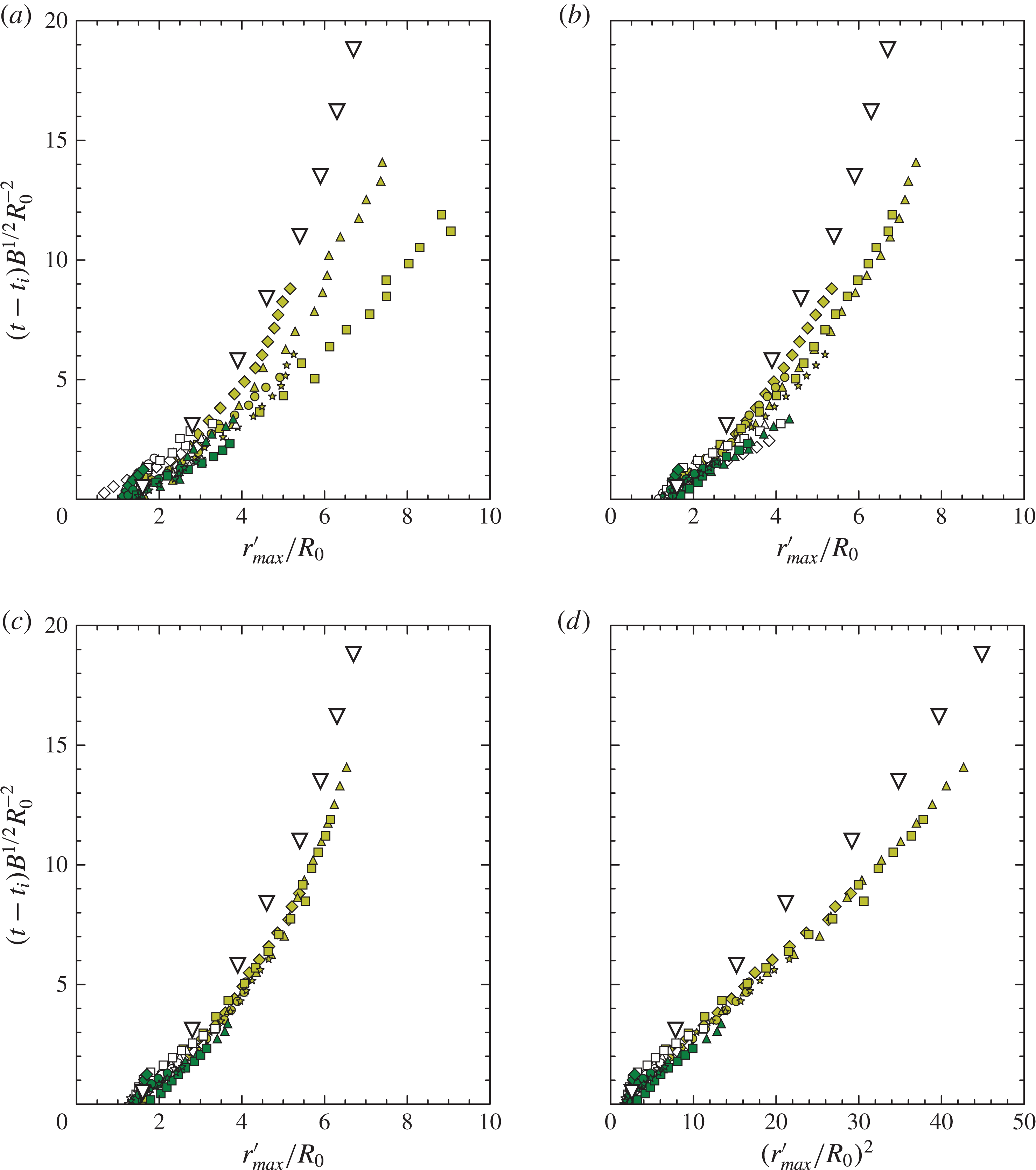
Figure 8 shows the same data plotted with the scaling of Lundgren et al. (Reference Lundgren, Yao and Mansour1992). This plot has also been used to illustrate the effects of taking different values of the buoyancy-thresholding parameter
 ${\it\epsilon}$
, see (3.4). It is evident that at lower values of
 ${\it\epsilon}$
there is greater scatter in the results, partly caused by azimuthal inhomogeneity and consequent variations in the centre of mass at these low values. At
 ${\it\epsilon}=0.8$
, however, the scaled maximum radii are in close agreement across all experiments. It was shown in § 2.3 that the scaling of figure 8 may be derived from the similarity solution, so the collapse of the data in figure 8(c) might be expected. However, this approach does give some additional insights.
Firstly, it highlights the differences in gravity-current propagation distance relative to the source length scale
 $R_{0}$
. Following Lundgren et al. (Reference Lundgren, Yao and Mansour1992), this length scale is the equivalent spherical radius of the impinging volume of fluid which, for the data here, is calculated from the fundamental flow parameters using (2.20). Domain constraints meant that all simulations were terminated when the absolute radius was of the order of one quarter of the horizontal domain extent. Thus, the absolute radius is similar for all flows, see figure 7. However, figure 8 shows that the flow propagation relative to the source scale is significantly greater for experiments L01–L05, in which the thermals fall a shorter distance, and consequently entrain much less.
Secondly, figure 8 also shows data from estimates of the radial propagation of a real microburst at Dallas Fort Worth (DFW) airport, made by Fujita (Reference Fujita1986). Lundgren et al. (Reference Lundgren, Yao and Mansour1992) replotted these data in their figure 3, demonstrating good agreement with their lab experiments (not shown), and the data imported here are taken from that presentation. Figure 3 of Lundgren et al. (Reference Lundgren, Yao and Mansour1992) shows radial growth during both the descent and gravity-current phases together, so for use in the present context the dimensionless impingement time of the DFW microburst has been estimated from the plot as
 $t_{i}/t_{0}\approx 4.5$
. With this estimate, it can be seen that the agreement of the DFW data with the LES results is likewise good. Thus, it appears that LES, lab experiments and estimates from an actual microburst all produce radial growth estimates that are in accord with one other, and hence with the similarity prediction (2.18).
Spread of the radial gravity current arising from thermal impingement. Data are identified as in figure 4. The data are plotted to compare with the scaling of (2.19). The inverted white triangles correspond to data from an actual microburst discussed by Fujita (Reference Fujita1986), and were taken from Lundgren et al. (Reference Lundgren, Yao and Mansour1992), figure 3. (a–c) Show results obtained for various values of the thresholding parameter
 ${\it\epsilon}$
, see (3.4), (a)
 ${\it\epsilon}=0.4$
, (b)
 ${\it\epsilon}=0.6$
, (c)
 ${\it\epsilon}=0.8$
. (d) Repeats the data from (c) but plotted against the square of the dimensionless radius, to demonstrate the expected
 $r\sim t^{1/2}$
spreading rate.

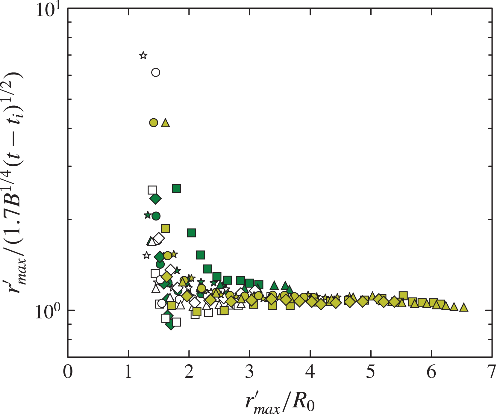
A final piece of information on the influence of the impingement zone may by obtained by replotting the data from figure 7(b) to show directly their departure from the similarity fit. Figure 9 shows the ratio of the radial scale to the similarity solution, plotted against dimensionless radius. This indicates that, for the large majority of the data, transition to the similarity solution takes place over approximately the length of one impingement radius
 $R_{0}$
.
The ratio of
 $r_{\mathit{max}}^{\prime }$
and the similarity solution
 $r_{\mathit{max}}^{\prime }=1.7B^{1/4}(t-t_{i})^{1/2}$
, plotted against the dimensionless radius
 $r_{\mathit{max}}^{\prime }/R_{0}$
. This demonstrates the rapidity with which the similarity solution is approached for gravity currents arising from thermal impingement.

4.4. Comparison with the similarity solution for
 $g^{\prime }h$

The analysis of § 4.3 demonstrated that the front propagation derived from thresholding the LES data is consistent with the analytical model, and also with laboratory measurements. However, the more diffuse nature of the upper interface, as discussed in § 4.2, means that the thresholding approach does not produce a similarly robust measure of the current depth. In this case, a more reliable metric for the depth is the integral depth scale
 ${\it\zeta}_{I}$
of the negative potential-temperature perturbation, see (3.6).
As well as defining the dynamical depth scale, (3.6) gives a slightly different perspective on the similarity solution (2.11b ). That is, it defines the depth through a relationship of the form
 $$\begin{eqnarray}g_{\mathit{max}}^{\prime }{\it\zeta}_{I}\sim (g/{\it\theta}_{a})\int _{{\rm\Delta}{\it\theta}<0}{\rm\Delta}{\it\theta}\,\text{d}{\it\zeta}.\end{eqnarray}$$
Similarly, the total buoyancy of an axisymmetric spreading current is
 $$\begin{eqnarray}B\sim (g/{\it\theta}_{a})\iint _{{\rm\Delta}{\it\theta}<0}2{\rm\pi}r\,{\rm\Delta}{\it\theta}\,\text{d}r\,\text{d}{\it\zeta}.\end{eqnarray}$$
Thus, if the current has only a weak radial potential-temperature structure, then the relationship
 $B\sim r^{2}g_{\mathit{max}}^{\prime }{\it\zeta}_{I}$
may be expected to follow approximately, from considerations of buoyancy conservation alone.
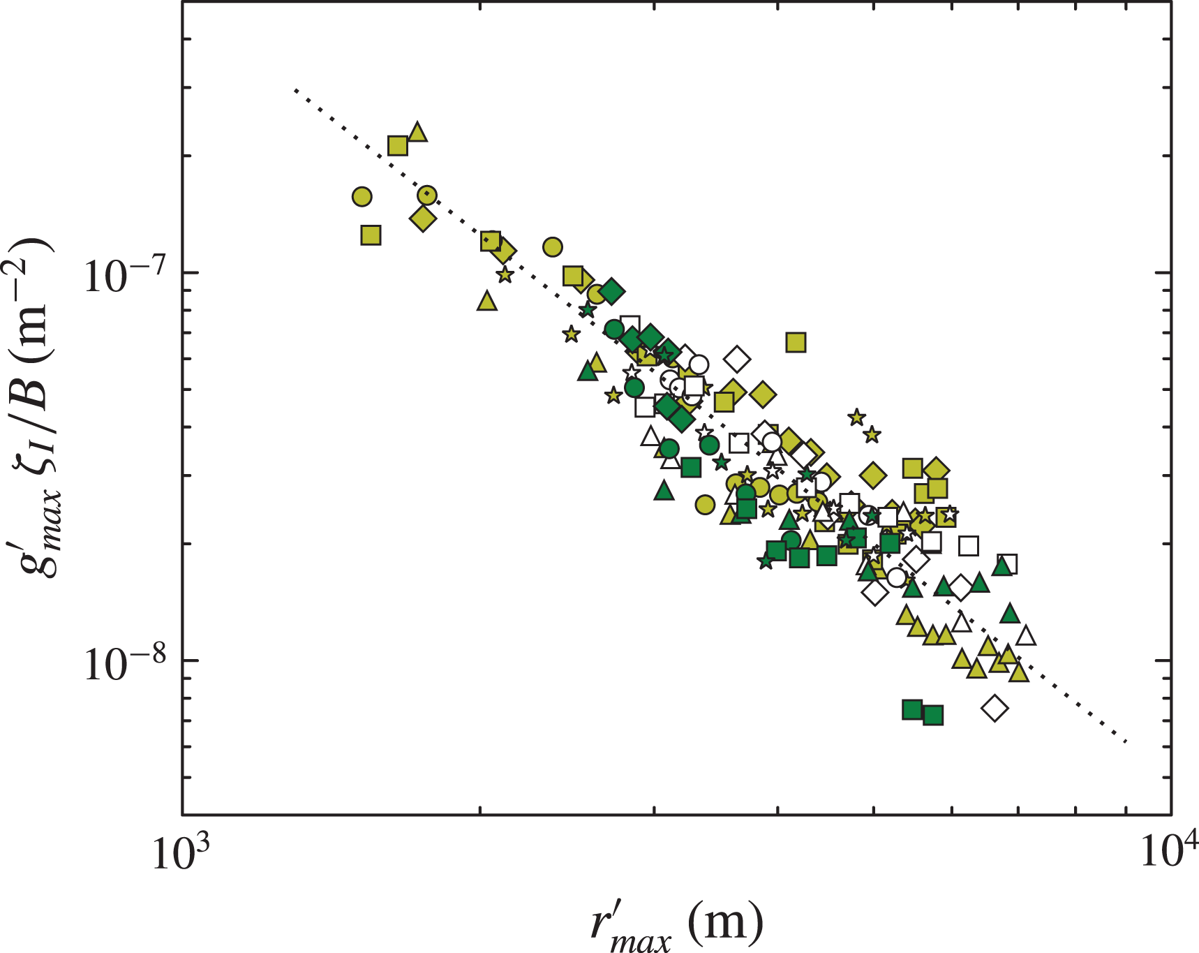
Figure 10 shows
 $g_{\mathit{max}}^{\prime }{\it\zeta}_{I}$
plotted to compare with (2.11b
). Only data from the post-impingement (
 $t>t_{i}$
) phase are shown, and it appears that these follow the scaling satisfactorily, with the quantitative relationship given approximately by
 $$\begin{eqnarray}g_{\mathit{max}}^{\prime }\,{\it\zeta}_{I}/B=0.5\,r_{\mathit{max}}^{\prime -2}.\end{eqnarray}$$
The product of integral depth scale
 ${\it\zeta}_{I}$
and maximum reduced gravity
 $g_{\mathit{max}}^{\prime }$
from the LES data in the post-impingement (
 $t>t_{i}$
) phase of the flow. Data are identified as in figure 4. The data are normalised by the buoyancy
 $B$
and plotted against the maximum radius
 $r_{\mathit{max}}^{\prime }$
, to compare with (2.11b
). The dotted line has equation
 $g_{\mathit{max}}^{\prime }\,{\it\zeta}_{I}/B=0.5\,r_{\mathit{max}}^{\prime -2}$
.

4.5. Quantifying entrainment to obtain the reduced gravity and depth
The analysis in §§ 2.2 and 2.3 shows that the unknown gravity-current entrainment function
 $f$
is present in the solutions for both the reduced gravity
 $g^{\prime }$
and the depth scale
 $h$
. To quantify entrainment from the data, it is simplest to examine the radial evolution of the reduced gravity. This is solely a function of
 $f$
, whereas the depth depends on
 $f$
and also has an additional
 $r$
dependence, see for example (2.15).
Based on (2.15b
), if the reduced-gravity scale
 $g^{\prime }$
and the measured maximum
 $g_{\mathit{max}}^{\prime }$
are assumed proportional, then the form of
 $f$
may be obtained by plotting
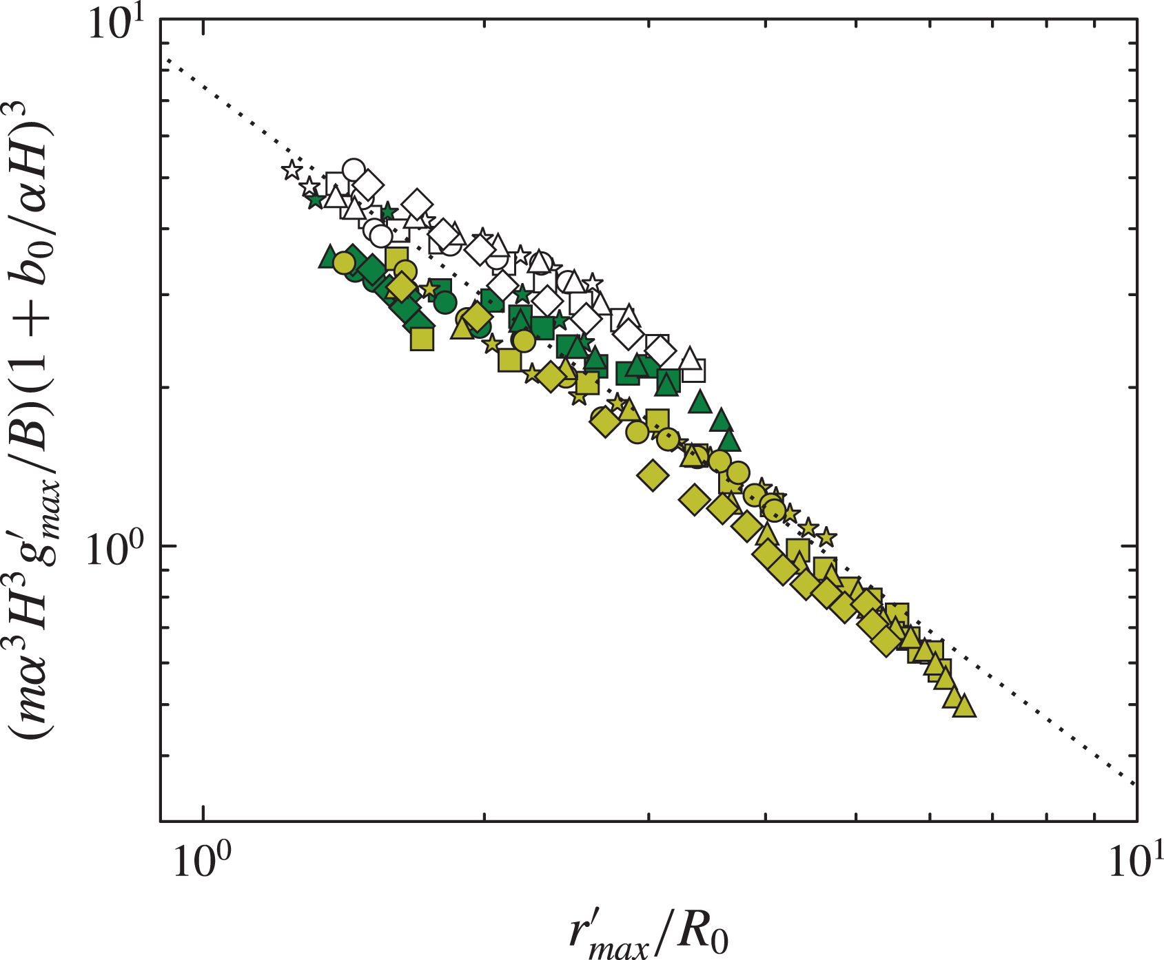
 $(m{\it\alpha}^{3}H^{3}g_{\mathit{max}}^{\prime }/B)(1+b_{0}/({\it\alpha}H))^{3}$
against
 $r_{\mathit{max}}^{\prime }/R_{0}$
. This is shown in figure 11. Also shown is the best fit to the data in the log–log plot. This has equation
 $$\begin{eqnarray}(m{\it\alpha}^{3}H^{3}g_{\mathit{max}}^{\prime }/B)(1+b_{0}/({\it\alpha}H))^{3}\approx 7.4(r_{\mathit{max}}^{\prime }/R_{0})^{-1.3},\end{eqnarray}$$
with a correlation coefficient of
 $-0.95$
. It is equivalent to
 $$\begin{eqnarray}f=(r_{\mathit{max}}^{\prime }/R_{0})^{1.3},\end{eqnarray}$$
if
 $g_{\mathit{max}}^{\prime }/g^{\prime }=7.4$
. The ratio of the maximum to the ‘scaling’ reduced gravity is much greater here than in the descending thermal. This may be a result of the different structures of these flows, since the vertical, convecting motion of the thermal will be more effective at creating mixing throughout the flow, in contrast to the gravity current, which has a stably stratified vertical structure in the mean.
Substituting these relationships into (4.3) then implies
 $$\begin{eqnarray}\displaystyle \frac{{\it\zeta}_{I}}{H} & = & \displaystyle \frac{1}{14.8}\left(\frac{r_{\mathit{max}}^{\prime }}{H}\right)^{-2}\left(\frac{r_{\mathit{max}}^{\prime }}{R_{0}}\right)^{1.3}m{\it\alpha}^{3}\left(1+\frac{b_{0}}{{\it\alpha}H}\right)^{3}\nonumber\\ \displaystyle & = & \displaystyle \frac{1}{14.8}\left(\frac{r_{\mathit{max}}^{\prime }}{R_{0}}\right)^{-0.7}\left(\frac{H}{R_{0}}\right)^{2}m{\it\alpha}^{3}\left(1+\frac{b_{0}}{{\it\alpha}H}\right)^{3},\end{eqnarray}$$
or
 $$\begin{eqnarray}m^{-1}{\it\alpha}^{-3}\left(1+\frac{b_{0}}{{\it\alpha}H}\right)^{-3}\left(\frac{R_{0}}{H}\right)^{2}\frac{{\it\zeta}_{I}}{H}=\frac{1}{14.8}\left(\frac{r_{\mathit{max}}^{\prime }}{R_{0}}\right)^{-0.7}.\end{eqnarray}$$
The depth data are plotted with this scaling in figure 12. Most of the scaled data lie within a range of less than one order of magnitude, and the radial dependence on
 $r_{\mathit{max}}^{\prime }$
is relatively weak. Nonetheless, the data cluster around the predicted line, the majority within a factor of two.
The maximum reduced gravity in the spreading phase of the experiments, plotted to compare with (2.15b
). The dotted line is the best fit, with equation
 $(m{\it\alpha}^{3}H^{3}g_{\mathit{max}}^{\prime }/B)\,(1+b_{0}/({\it\alpha}H))^{3}=7.4\,(r_{\mathit{max}}^{\prime }/R_{0})^{-1.3}$
.

The integral depth scale in the spreading phase of the experiments, plotted to compare with (4.7) shown by the dotted line.

5. Conclusion
Results have been presented of the LES of negatively buoyant thermals. The associated potential-temperature perturbation has been used to track these flows as they descend, impinge on the ground and spread outward. Existing similarity solutions for the propagation of thermals and axisymmetric gravity currents have been combined into a model of this flow.
Thermal descent is observed to follow closely the similarity predictions of mean velocity and reduced gravity, upon the addition of a virtual origin. This contrasts with the conclusion of Morton (Reference Morton and Smith1997), who noted a large variability in the mean behaviour of laboratory thermals. The transition of the flow through the impingement region in the LES appears reasonably smooth. The major phase of flow adjustment seems rather to be the post-release phase of the thermal, which is analogous to the ‘slumping’ phase of lock-release gravity currents, and this prior adjustment of the flow before impingement may contribute to the smooth transition.
The analytical model defines the speed of the gravity current in terms of the conserved buoyancy. The impingement time scale from the thermal model allows the time-dependent radial extent of the spreading flow to be related to the buoyancy, release height and radius of the buoyant parcel which initiates the flow. The similarity solution has been shown to anticipate the flow scaling identified by Lundgren et al. (Reference Lundgren, Yao and Mansour1992), and so to relate the present numerical results to corresponding lab experiments, and thence to observations of an actual microburst.
The model cannot predict the magnitude of entrainment by the gravity current, although it does allow the problem to be reduced to finding a functional relationship between dimensionless variables. The experiments have verified the theoretical framework, and gravity-current entrainment has been shown to correlate well with dimensionless radius. This has enabled separate expressions for the gravity-current depth and reduced gravity to be obtained.
The present study has produced a model of the downdraught through all the stages following initiation. This will enable anticipated future work to concentrate on the later stages of the problem, and examine the impingement flow structures and gravity-current behaviour in more detail. The suppression of surface heat flux in the present model configuration has facilitated comparison with water-tank experiments where buoyant effects are produced through salinity variation. However, the effect of surface heating is another area which should be investigated in future.
Acknowledgements
A. A. Hill’s help with the LEM is gratefully acknowledged. Thanks are also due to C. J. Smith for advice on the original ‘warm bubble’ experiments, and to B. J. Shipway for help with the animations.
Supplementary movies
Supplementary movies are available at http://dx.doi.org/10.1017/jfm.2015.484.