

Introduction
The simulation of materials at the atomic scale is almost as old as the first computer and predates even the use of punched paper tape or decks of cards from the early computing experience. Motivated by the need to understand irradiation damage, the computer simulation of atomic processes in matter started growing in the 1950s,Reference Gibson, Goland, Milgram and Vineyard1 and it continues to grow. While the last MRS Spring Meeting bore witness to a renewed interest in nuclear materials and irradiation damage (e.g., Symposia U,2 RR,3 and XX4), the power and scope of atomistic simulation in materials science has widened enormously. It now embraces fracture, phase changes, statistical thermodynamics, the evolution of microstructure from point defects to dislocations, biological membranes, and organic/inorganic interfaces. In the field of atomistic simulation, we strive to gain insight into the behavior of real materials under the constraints of contemporary computing power.
In the 1930s, Coulson demonstrated how quantum mechanics give rise to interatomic forces in molecules,Reference Coulson5 laying some of the foundations for what we now know as tight-binding models. Nevertheless, in the early days of computer simulation, very crude models of interactions between atoms were used for computational simplicity, in which the total energy was described as a sum of pairwise potentials, V:
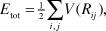
where Rij denotes the distance between the nuclei at positions labeled i and j. It was not until the 1960s that computer power, and concepts in solids, had advanced enough for quantum theory to be put into practice for interatomic forces in condensed matter.Reference Harrison6 This led to some of the successful developments in the modeling of interatomic forces with many-body potentials, described here.
Several trends and branches can be discerned in modeling interatomic forces today. A central pillar of the field remains the Hohenberg-Kohn-Sham density functional theoryReference Hohenberg and Kohn7, Reference Kohn and Sham8 (DFT) using a local density or density gradient, usually referred to as a “generalized gradient,” approximation (LDA or GGA) to quantify the energy of exchange and correlation between electrons. The idea of the LDA is that the electrostatic energy of a sea of electrons is less than the electrostatic energy of a classical continuum of charge because the electrons keep out of each other’s way. Nevertheless, the difference in energy per electron is assumed to be the same at each point in the varying density as it would be if the electrons there were part of a uniform density. The electrostatic energy of electrons as a function of a uniform density has been calculated to good accuracy, and with the LDA, its functional form is used directly for the inhomogeneous density. The GGA is a refinement that makes the energy also a functional of the density gradient at a point. With the computational resources available to most laboratories, DFT provides an acceptable accuracy of energies and structures over the widest range of materials. It is often referred to as an ab initio method, because no empirical parameters are involved, although its approximate nature should not be forgotten. For some years to come, DFT will remain the method of choice for mainstream simulations of low energy (a few eV per atom) and short times (a few ps), or for high throughput and a few hundred atoms. Hence, there is ongoing research to make DFT faster, more efficient, and more user-friendly by increasing the functionality of codes and optimizing the method for the next generation of supercomputers.
Universal binding energy relation
In the early 1980s, Rose et al. showed that, if properly scaled, energy versus distance relations for a wide variety of materials and types of distortions could be reduced to a single universal binding energy curve that could be accurately fit by a Rydberg function (J.H. Rose, J.R. Smith, F. Guinea, J. Ferrante, Phys. Rev. B 29, 2963 (1994)). The systems included diatomic molecules and metallic and covalently bonded solids, and the distortions included uniform contractions and expansions of crystalline solids and diatomic molecules, cleavage along crystal planes, and chemisorption of atoms onto surfaces. Abell developed a theory that explained this apparent universality in bonding relations among otherwise disparate systems that helped lead to Tersoff’s functional form for his bond order potentials (G.C. Abell, Phys. Rev. B 31, 6184 (1985)). The universal bonding energy relation has also provided a convenient function that can be used to develop, fit, or evaluate potential energy expressions.
Because DFT is inadequate in some situations (typically surface processes and adsorption of atoms) and for some materials (typically oxides of transition metals to the right of the periodic table, or lanthanides and their compounds), a second branch of current research is concerned with incorporating more exactly the correlation between electrons into the simulation methods. There are simple, semi-empirical extensions to DFT such as LDA+U, which aim to correct its most serious fault, which is to count the energy of interaction of each electron with the Coulomb potential of itself. Here “U” refers to the “Hubbard U” parameter that is included in the functional, following ideas of Zaanan and co-workers.Reference Anisimov, Zaanen and Andersen9 The absurdity of this error is obvious, but it is not trivial to eliminate. Its importance becomes negligible in the limit of a delocalized electron, whereas it can only be exactly evaluated for an electron in a completely localized orbital, and unfortunately the exact many-electron wave function does not make a clear distinction between these extremes. A number of methods have been or are being developed to treat more exactly electron correlation in general, including methods that could, in principle, be converged systematically to the exact answer, such as the Quantum Monte Carlo method. These are all computationally expensive methods of calculating the total energy, and the difficulty of calculating accurate forces on nuclei raises the resources barrier still further.
Despite all the research on the speed and accuracy of first-principles methods, in order to satisfy the ambition of meaningful results for systems of up to hundreds of millions of atoms and to explore the complexity of emergent phenomena of such length scales, or to explore timescales required for calculating thermodynamic properties at high temperature, there remains a need for relatively simple many-body potentials, trading some quantitative accuracy for speed. Many-body potential refers to an explicit function that describes the potential energy of an assembly of atoms as a function of their positions, rather than a method that requires a differential equation to be solved every time. DFT and the more advanced quantum mechanical methods for calculating total energies and forces mentioned previously have a role to play in helping to generate such functions or fit their parameters.
There have always been at least two general approaches to generating models for many-body potentials in materials. Broadly speaking, the first is to write down a convenient functional form as a sum over atomic nuclei. The function should involve a few, perhaps only one or two, shells of nearest neighbors and perhaps also the angles they subtend at the nucleus.Reference Keating10 Its parameters are fitted to experimental data and perhaps also fitted to data calculated by a reliable ab initio method. The second approach (e.g., in ab initio pairwise potentials, some classes of ionic models, embedded atom potentials, bond order potentials, and tight-binding models) is to derive a functional form directly from DFT and not necessarily with the usual attendant approximation of LDA or GGA. This approach covers a range of materials and models, but in practice, there is usually some empiricism involved even in the second approach. Until recently it was believed that the second approach is bestReference Finnis11 because it has a more physical basis. However, a third class of methods has emerged recently, motivated by the inaccuracy of the previous simpler models for many purposes. These methods are based on information theory, employing neural networks or a Bayesian reconstruction of the energy versus local atomic configuration. Such models require minimal a priori assumptions about the functional form of the potentials, at least at short range.Reference Behler and Parrinello12, Reference Bartók, Payne, Kondor and Csanyi13
A fruitful strategy for modeling large, inhomogeneous systems with atomic-scale detail is to start by recognizing that usually only a small part of the system needs an accurate quantum mechanical treatment, perhaps with DFT, such as the tip of a crack, a dislocation or a point defect, or a place where chemical bonds are being made or broken. Most of the atoms in the system are in a local environment very similar to bulk, perfect material, as is typical in a strained crystal. This leads to the concept of embedding a small region where electrons are explicitly treated by a quantum mechanical calculation within a region where the atoms are classical interacting particles. There are several such QM/MM (quantum mechanics/molecular mechanics) methods, as they are often called. Much of the research on this approach aims to devise consistent ways of matching quantum mechanical and classical regions as seamlessly as possible, so as not to violate Newton’s laws of motion for any of the nuclei and to define a total energy for the heterogeneous system. However, a description of such embedding methods is beyond the scope of this article.Reference Csanyi, Moras, Kermode, Payne, Mainwood and De Vita14 This article elaborates on the models mentioned earlier and attempts to summarize for non-specialists their ingredients, virtues, and drawbacks.
Pseudopotentials
The concept of pseudopotentials, developed in the 1950s,Reference Phillips and Kleinman15 has nothing directly to do with interatomic potentials in the sense of Equation 1. Nevertheless, it provided a way to derive pairwise interatomic potentials in simple metals. A pseudopotential is the effective potential acting between an electron and a positive ion, not the potential acting between ions or atoms. It is an “effective” potential seen by an electron, in the sense that an ion or an atom is not really a simple entity, but a collection of particles interacting with each other and with the other nuclei and electrons in the material. A pseudopotential therefore is constructed such that the many dynamic interactions between a positive ion and an electron are replaced by a single static interaction centered on the nucleus of the ion, which replicates the ion’s effect on an external electron. The electrons within the positive ion itself are referred to as core electrons, and their energies and mutual interactions are not treated explicitly. That is a useful approximation, because it is practically only the dynamics of the outer electrons of the atoms, the “valence” electrons, that determine chemical bonding and mechanical properties of a material. On that basis, it proved possible in the 1960s to introduce a simple pseudopotential that quantitatively explained the band structure of crystals.
Furthermore, the concept could explain why the electrons in simple metals appear to be nearly free.Reference Harrison6, Reference Cohen, Heine and Weaire16, Reference Harrison17 A pseudopotential looks the same as the potential of an ion, namely –Z/R, where Z is the charge, from the point of view of electrons at a distance from the nucleus of r > r c, where the core radius r c is large enough to enclose the entire density of core electrons. However, within this core radius, the deep Coulomb well is replaced by a much shallower potential. The wave function of a single electron ψ(r, θ, ϕ), where r, θ, and ϕ are the usual set of spherical polar coordinates of a certain energy E acted upon by a pseudopotential, looks the same as in the real potential for r > r c, but within the core radius, the electron has a higher potential energy V(r) and a lower kinetic energy  . The latter general relation between the kinetic energy and the curvature of a wave function means that the “pseudo” wave function is smoother than the real one inside the core of the ion. The electrons scattered by a pseudopotential may appear more nearly free than one would expect, although the scattering properties of the pseudopotential are the same, by construction, as the real potential.
A pseudopotential should reproduce the scattering properties of a real potential accurately over the energy range of interest for valence electrons in a solid, and that proved to be possible only when the pseudopotential was a “non-local” operator. In practice, this usually means that the pseudopotential depends on the angular momentum of the scattered electron about the nucleus. The idea here is that a wave function can be expanded about an atomic nucleus as a linear combination of terms such as  , the product of a radial function and a spherical harmonic, where m is the usual integer that labels the angular dependence of the spherical harmonic. The simplest non-local construction of a model potential introduced a different core radius and a different constant potential within the core for each angular quantum number ℓ, which required several parameters to be fitted or calculated. Non-local pseudopotentials are still widely used for the fully self-consistent calculation of electronic structure and total energies in condensed matter, most often in conjunction with DFT. However, for the purpose of model building, their essential property in simple metals, such as Li, Na, Mg, and Al, is the weak perturbation they represent to a free electron gas, in which they form pseudoatoms. Harrison probably made the first calculation of a phonon spectrum from first principles (with no fitting parameters) for aluminum using a simple pseudopotential and second-order perturbation theoryReference Harrison18—equivalent to a density-dependent pairwise interatomic potential (see later in text). With no adjustable parameters, the accuracy in comparison to neutron diffraction data was only qualitative. However, by allowing one parameter to vary, he achieved a good fit to the experimental data.
Pseudoatoms
Pairwise interatomic potentials in simple metals are associated with pseudoatoms. A pseudoatom resembles an atom; it consists of a positive ion surrounded by a cloud of electrons that screen it. The difference between a pseudoatom and a real atom is that the pseudoatom is part of a condensed system, and the screening electrons are not bound to it as they are in free atoms but are free to move through the material and screen other ions because they are conduction electrons. Nevertheless, the pseudoatom is a distinct entity, which is defined by the electron density. This is because when the ion moves, it carries the local profile of electron density with it, just as an atom with bound electrons would. If we place a positively charged ion of a simple metal, for example Al3+, into a free electron gas, it is screened by the spherically symmetric density of electrons that appear around it, which moves rigidly with the ion. The significance of the weakness of the perturbation presented by pseudopotentials in a free electron gas is that the screening of ions is linear, such that the density of electrons induced by screening an assembly of such ions should be just a superposition of the densities of the individual pseudoatoms, in which the spherical screening densities overlap. In this sense, the pseudoatoms making up the material (or liquid) preserve their spherical shape under rearrangement of the positions of the ions.
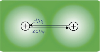
Feynman and othersReference Ehrenfest19–Reference Hellmann21 have taught that even in quantum mechanics, the energy change of a material under a rearrangement of the positions of the nuclei of its atoms is simply given by integrating the classical electrostatic force on those nuclei along their paths, provided the electrons alone show quantum mechanical behavior and the ions, treated as classical particles, are not moving too supersonically. Within the pseudoatom picture, the force on an ion is nothing more than the sum of the electrostatic forces exerted on it by all the other pseudoatoms. Thus, if within the sphere of radius Rij about the nucleus of atom j the spherically symmetric screening charge amounts to −Q, while the ions i and j each carry charge Z, the net force on ion i due to pseudoatom j is simply Z 2 / Rij − Z ·Q / Rij (see Figure 1). Hence we can describe the energy changes by using a sum of pairwise potentials, which can be calculated for simple metals, in principle, without fitting parameters to any mechanical properties of the elements involved. The total energy of the system therefore has the form:

The pairwise force acting on a pseudoatom. The force on each nucleus is the sum of the Coulomb repulsion due to the other nucleus and the attraction due to the spherical screening cloud of electrons (indicated by the shading) centered on the other nucleus. Note: Z, atomic charge; Q, screening charge; Rij, distance between nuclei at positions i and j.

in which a complicated but well-defined function of density F (ρ) describes a large part of the energy under volume changes of the system, besides the pair potential. The density dependence of the pair potential arises because the radial density of a pseudoatom is a function of the mean density ρ of conduction electrons, that is, the density of the original free electron gas into which the ions were placed. FinnisReference Finnis11 reviewed the detailed formulas and their derivations.
The reason for the limited accuracy of such ab initio pair potentials is mainly the linear screening approximation, which indeed makes them useless or nearly so for metals in which the d-states contribute to the rearrangement energy, including all the transition metals. A more subtle problem of the linear screening approximation is that the function describing the screening of ions depends on the density ρ of the homogeneous free electron gas that screens them. Recalling that ρ is the density of the homogeneous electron gas upon which the application of perturbation theory gives Equation 2, it is not surprising that the formalism cannot correctly describe the energy associated with inhomogeneous changes in density within the system on the mesoscale, such as that which occurs across solid-liquid interfaces, compression waves, or, in the most extreme case, through a surface from solid to vapor. In reality, the shapes of pseudoatoms, if the concept is retained, must depend on the local environment. This concept was built into the developments described later in the text.
Quasiatoms, effective medium theory, and embedded atom models
It might seem a short step from Equation 2, known in the 1960s, to defining the density in a local way and thereby overcoming the previously mentioned difficulties. Nevertheless, over a decade elapsed before Stott and Zaremba published their theory of quasiatoms,Reference Stott and Zaremba22 a forerunner of effective medium theoryReference Norskov and Lang23–Reference Jacobsen, Norskov and Puska25 (EMT) and of the more empirical and now more widely known embedded-atom methodReference Daw and Baskes26, Reference Daw and Baskes27 (EAM) for modeling interatomic forces in metals. This period coincided with the establishment of DFT as a remarkably accurate tool for first-principles calculations, which could be used to benchmark new models, and which became increasingly useful for generating data for fitting their empirical parameters (see the sidebar on Parameter fitting).
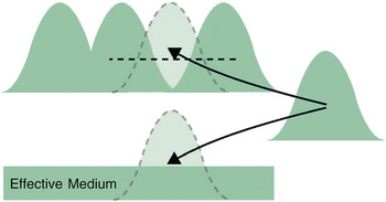
Quasiatoms are very much like pseudoatoms, but without the approximation of linear screening. The basic idea is to consider the energy change when a free atom is added to a uniform electron density ρ as a very first approximation to the energy change ΔE when it is added to a material at a point where the inhomogeneous local electron density is ρ (see Figure 2). The former energy can be calculated once and for all with DFT, without the approximation of linear screening. The EMT derived by Jacobsen et al.Reference Jacobsen, Norskov and Puska25 is more subtle than that, since it exploits the variational principle to determine the optimum value of the uniform density ρ, which should clearly be some kind of a weighted average over the volume occupied by the embedded atom. Corrections are then added to take into account the actual local atomic configuration. The derivation respects quantum mechanics up to a point; for example, one small term in ΔE can be the difference in the sum of the single electron energies in the material before and after the atom has been inserted. However, this term is neglected because it would enormously increase the computational cost of the resulting expression for the energy. The bottom line is that, in its simplest form, the energy looks like
Parameter fitting
Experienced developers of potential energy functions use different strategies to fit parameters in the mathematical expressions. Some researchers try to fit as many properties as possible, which requires a potential function with numerous adjustable parameters. Others try to strategically fit a few key properties and structures and rely on a physically motivated functional form to properly describe properties outside of the fitting database. In general, for solids it is important to include in the fitting database structures that have different atomic coordination such as bulk crystals and point defects such as vacancies and interstitials, elastic properties, and, if possible, thermodynamic quantities such as melting points and thermal expansion coefficients. It is also critical to ensure that the intended structures, including amorphous structures, are the lowest in energy.

Schematic illustration of the concept of embedding an atom within the average electron density, indicated by the horizontal dashed line, at its target position in the host.

This is the form of the EAM. Notice that compared to Equation 2, the density is defined locally at each atomic site, but it has disappeared from the pair potential. The density ρi in this formalism is calculated by summing contributions from neighboring atoms:

For simplicity, it is assumed in this example that only one element is involved. The function φ is generally treated as short-range and fitted empirically to energy data, together with the pairwise function V. The first term in Equation 3, the embedding term, is cohesive in nature; thus the function f is negative and increases in magnitude with the density and number of neighbors.
Tight binding
A completely different approach to generating many-body potentials, appropriate for transition metals but not for nearly free electron like metals, is based on the tight-binding model of electronic structure, or the linear combination of atomic orbitals (LCAO) method. Tight-binding works with a sparse matrix, the Hamiltonian matrix Hi αjβ, whose elements are the overlap integrals of orbitals α and β on neighboring atoms, and they can be parameterized once and for all for the material under study. Curiously, in its most simplified form, described later, this leads to a total energy that looks exactly like Equations 3 and 4, although the physical interpretation of the terms is different. Tight binding is something of a misnomer, conceived because the Schrödinger equation for the electrons is solved with a basis set of localized orbitals; but the electrons are not “tightly bound” to their atoms because the orbitals overlap, so every electron in the material occupies a delocalized state that is a linear combination of these orbitals (hence the term LCAO).
There are many flavors of tight-binding models that have been developed for transition metals, semiconductors, and ceramics. They are most conveniently derived from the expression for total energy given by DFT through a sequence of approximations, as discussed in detail elsewhere.Reference Finnis11 A key quantity in DFT and tight-binding theory is the sum of effective single-particle energies, which can be thought of as the sum of the energies of each electron in a mean field of the others and of the ions. It is also related to the electronic density of states D(E) by
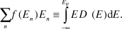
This is the zero Kelvin limit, where E F is the Fermi energy, and f(En) = 2 (electrons of up and down spin) if En is below the Fermi energy, otherwise it is zero. The extension to finite temperature is straightforward. The above term contains a large part of the total cohesive energy, and indeed it has long been known to explain the trends in cohesive energy and crystal structure of the transition metals across the periodic table.Reference Friedel28–Reference Pettifor30 It is a common and useful approximation with tight binding to subtract from Equation 5 the corresponding expression for free atoms, defining a total bond energy, which in its simplest form is:
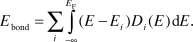
The energy Ei is that of the electron orbital, usually a d-orbital, in separated free atoms, and Di(E) is the local density of states on atom i. The remainder of the energy, including the correction for double counting in Equation 5 of electron-electron interactions, is then approximated by a sum of pairwise potentials.
The explicit evaluation of Equation 6, either with DFT or more cheaply and approximately by tight binding, can be done by solving the Schrödinger equation for a single electron to obtain the eigenvalues En. However, there are smarter approaches to evaluating Equation 6, which, in the spirit of interatomic potentials, avoid the need to solve any differential equations for the energies of electronic states. These approaches are founded on the ideas that (1) the important information about the density of states is already contained in its lowest moments:
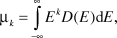
and, (2) these moments can be evaluated directly from the Hamiltonian matrix that embodies the tight-binding model, which itself can be parameterized once and for all for the material under study. The first moment μ1 simply locates the centroid of D(E),  is proportional to its width, μ3 describes its skewness, and so forth. There is extensive literature on how to obtain moments from the Hamiltonian matrix and how to reconstruct a model of D(E) from them, including an elegant and widely used approach that shortcuts the explicit evaluation of individual moments by using the Lanczos method, or recursion method.Reference Friedel and Ziman29, Reference Cyrot-Lackmann31–Reference Obata and Masuda Jindo39 A direct offshoot of these ideas has led to bond-order potentials, described in detail elsewhere in this issue.
The simplest approximation includes only the second moment of D(E), which has a contribution from each atomic site. These contributions are constructed by summing the matrix elements of the Hamiltonian to neighboring atoms:
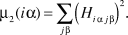
The attractive contribution to the total energy, which to a first approximation scales as  , can be further simplified by assuming just one orbital per atom, in which case it can be written in the form
 as in Equation 3, where now the physical origin of this term is identified by the relation

Like the EMT or EAM approach, in practice, for the second moment model, the terms in Equations 3 and 4 are parameterized in an empirical way.Reference Cyrot-Lackmann31, Reference Ducastelle32, Reference Finnis and Sinclair40–Reference Allan and Lannoo42 Unlike the EMT or EAM approaches, however, tight-binding methods also enable a systematic hierarchy of models of increasing complexity and accuracy right up to the level of self-consistent DFT. It is indeed necessary to go beyond Equations 2, 3, and 4 for all but the most qualitative simulations. For example, parameters for Equations 3 and 4 can be fitted to elastic constants in many metals, but not always (e.g., it is impossible to fit these expressions to cubic elastic constants with a negative Cauchy discrepancy C 12 − C 44, as in Ir and some intermetallic alloys).Reference Nguyen-Manh, Vitek and Horsfield43 They are also unreliable for predicting the energy differences between crystal structures. For example, it is now known that the physical origin of the difference between the energies of bcc (body-centered-cubic) and fcc (face-centered-cubic) crystals requires a model in which μ4 is correctly reproduced, and the subtle fcc-hcp (hexagonal close-packed) energy difference requires accuracy to the level of at least μ6.Reference Drautz and Pettifor44
Self-consistency and extended ionic models
A model is generally regarded as self-consistent if in some sense it includes the effect of the redistribution of electrons that accompanies a change in the positions of atoms. Fortunately, there is a variational principle that tells us that the effect on the total energy is only second order in the amplitude of this redistribution, so self-consistency is not always as important as one might expect. Even omitting the second-order terms in the electronic redistribution can lead to acceptable models; this is the case for simplified EMT approaches, in which the electron density can be treated as a superposition of rigid atomic charge densities. In some models, a second-order level of self-consistency may be implicit, as in the density dependent pair potentials described previously. Otherwise, it may be treated explicitly by including, in addition to the positions of the nuclei, auxiliary variables, coupled to the nuclear positions, whose values have to be determined during equilibration or dynamics.
Perhaps the oldest and simplest example is the shell model of an ionic crystal, in which the ions carry a polarization variable either in the form of a point dipole or a spherical charged shell attached by a spring to the nucleus.Reference Dick and Overhauser45 The values of these variables must be determined self-consistently by minimizing the energy. Since electrons move much faster than sound, the Born-Oppenheimer principle dictates that this energy minimization should be carried out at the instantaneous positions of the ions.
While this was an improvement of the first-order ionic model of Born, its inadequacy became apparent in the calculations of elastic constants. If inversion symmetry is preserved on the ions within a homogeneously strained crystal, they remain unpolarized, and therefore the interatomic potential remains pairwise. As a consequence, the elastic constants in cubic crystals would have to satisfy the Cauchy relation for pairwise potentials, C 12 = C 44, instead of what we find for the simplest ionic oxide, MgO, in which experimental values are C 12 = 95.2 and C 44 = 155.7 GPa.Reference Zha, Mao and Hemley46 The problem can be dealt with by adding physically motivated degrees of freedom to the possible distortions of the oxygen ions, such as breathing or compressible shells.Reference Marks, Fabris and Finnis47, Reference Marks, Finnis, Harding and Pyper48 More sophisticated models of oxides also account for quadrupole polarizability and/or include short range modification of the polarizabilities by the local atomic configuration.Reference Wilson, Huang, Exner and Finnis49–Reference Jahn, Madden and Wilson51
Charge transfer between atoms in a material can also be included in a semi-empirical manner as an additional variable that equilibrates a surrogate chemical potential of the electrons,Reference Streitz and Mintmire52 although since the charge on an ion in a solid is not uniquely defined, at least some of the effect of charge transfer may already be captured in the dipole polarizability.
Information theory and outlook
Many-body potentials have become more varied and sophisticated, but considerable insecurity remains about how transferable or robust they are. Large databases of energies and forces for different crystalline and liquid structures are readily generated with first-principles calculations, to supplement the experimental data used for fitting parameters. However, the dangers of overfitting are well known. The more parameters that are used in a fit, even if the underlying functional forms are physically sound, the larger the error is likely to be when a structure very different from the “training set” is encountered. Anyone who has fitted polynomials of various orders to a set of data points on an x-y graph will see how this happens: a high-order polynomial will extrapolate or interpolate to greater nonsense than a simple linear or quadratic fit. The problem has been addressed in the present context by Frederiksen et al.,Reference Frederiksen, Jacobsen, Brown and Sethna53 who applied a Bayesian approach for the first time to quantify the error in the predictions of a fitted many-body potential. This is a more satisfactory procedure than reporting the root-mean-square error on a sample set of structures, since there are different views on the number of samples that should be in a training set and the number in a test set. Subsequently, the use of information theory has expanded to include the actual generation of potentials. This is an exciting new development for the field.
Two approaches based on information theory have been particularly fruitful: the neural network potentials of Behler and co-workersReference Behler and Parrinello12 and the Gaussian Approximation Potentials (GAP) of Csanyi’s group.Reference Bartók, Payne, Kondor and Csanyi13 For brevity, a description of the former is omitted here, since the methods have much in common. They both start from the assumption that the total energy can be written in the form of a sum over local, atom-centered energies:

The local environment can thereby be modeled, while any interactions of range beyond R c have to be treated by explicit functions, for example the Coulomb interactions in ionic crystals, as they are in traditional methods.
The GAP approach then works as follows. The complete atomic density in the neighborhood of an atom can be expanded to a desired accuracy in a set of three-dimensional functions, labeled λ. The expansion coefficients fitted for a member labeled N in a set of perhaps a few hundred different reference configurations are denoted as b(N, λ). The energy of the atom centered in a new configuration i is then evaluated as a weighted sum of the energies of the reference configurations:

The parameters α(N,M), rather than simply forming a diagonal matrix (N = M) as one might expect, are specially constructed to compensate for correlations between different reference structures using a Bayesian methodology.Reference Bartók, Payne, Kondor and Csanyi13, Reference MacKay54 The choice of these and the Gaussian spread parameters θλ is discussed in the literature.Reference Bartók, Payne, Kondor and Csanyi13 Since it is firmly based in information theory, the method also provides an estimate of the error. It has proved to deliver DFT accuracy at a tiny fraction of the cost.Reference Bartók, Payne, Kondor and Csanyi13 Transferability far away from the energy landscape of the “training set” is always likely to be a problem, but perhaps with physically based or reasonably good many-body potentials as a zeroth approximation, functions such as GAP will provide a systematic way of chipping away the remaining errors.
Acknowledgments
The author is especially grateful to Volker Heine for sparking his interest in this subject and for stimulating conversations over many years.