





1. Introduction
The motion of a small body moving along the axis of a rotating fluid is a classical problem in fluid dynamics (Taylor Reference Taylor1922). When the translation speed
 $U$
of a body of radius
 $a$
is slow compared with the rotation rate
 $\varOmega$
(the low-Rossby-number regime,
 $\textit{Ro}=U/(a\varOmega )\ll 1$
), columns of fluid form ahead of and behind the body that are dragged along with the body; these columns are called Taylor columns. Theoretical treatments of this flow have relied on various idealisations in order to make the analysis tractable. These include neglecting viscous terms, assuming that perturbations from solid-body rotation are small so that the equations may be linearised, assuming an asymptotically steady state and that the length scale of the body is small compared with the distance to any container boundary (Grace Reference Grace1922; Morgan Reference Morgan1951; Stewartson Reference Stewartson1952; Childress Reference Childress1964). In many analytical studies, several different values of the critical translation speed for the formation of Taylor columns were obtained. Lighthill (Reference Lighthill1967) and Bretherton (Reference Bretherton1967) ascribed the Taylor blocking phenomenon to the propagation of inertial waves from the body. The dye-visualisation experiments of Long (Reference Long1953) suggested that there are no waves propagating ahead of the body, but this has been disputed (Benjamin Reference Benjamin1970; Stewartson Reference Stewartson1970), and in his review article Long (Reference Long1972) suggested that the problem lies with the inconsistency of linearising the problem and casting it in an axially unbounded setting with the upstream velocity field assumed to be in solid-body rotation. The theoretical considerations of Long (Reference Long1953) and Benjamin (Reference Benjamin1970) are inviscid, while Stewartson (Reference Stewartson1970) considered both viscous and inviscid settings, finding a variety of inconsistencies associated with other model idealisations and noting that no convincing way had yet been found of making the solution unique and at the same time relevant to experimentally realisable flows.
Benjamin (Reference Benjamin1970) noted several inconsistencies between the experiments of Pritchard (Reference Pritchard1969) and theories implementing the hypothesis of undisturbed upstream flow from Long (Reference Long1953). Pritchard (Reference Pritchard1969) showed evidence of forward influence in the flow ahead of a translating sphere at Rossby numbers much higher than the limit suggested by Long (Reference Long1953), based on the assumption that the flow upstream is steady with uniform axial and angular velocities so that the governing equations reduce to a linear equation for the streamfunction. For
 $\textit{Ro}\ll 1$
, Benjamin (Reference Benjamin1970) suggested that the theory was sound and consistent with the observation of columns of fluid pushed ahead of and drawn behind the body (Taylor Reference Taylor1922), but was concerned that if
 $\textit{Ro}$
is not particularly small then the equations become intrinsically nonlinear. Long (Reference Long1953) detected no forward effect in experiments for
 $\textit{Ro}\gt 0.23$
, whereas Pritchard (Reference Pritchard1969) reported upstream blocking for
 $\textit{Ro}\lesssim 0.7$
and the presence of a more feeble type of columnar disturbance up to
 $\textit{Ro}\approx 2$
. By blocking, Pritchard (Reference Pritchard1969) refers to the situation where a quantity of dyed fluid placed in front of the sphere is pushed ahead of it for all time, and the feeble (a term used by Benjamin (Reference Benjamin1970)) situation corresponds to a forward influence extending far upstream but dyed fluid ahead of the sphere does not remain there for all time.
The inviscid theoretical approaches (e.g. Grace Reference Grace1922; Morgan Reference Morgan1951; Stewartson Reference Stewartson1952; Long Reference Long1953; Benjamin Reference Benjamin1970) are in line with the original theory from Taylor (Reference Taylor1922). Taylor (Reference Taylor1922), however, realised the problem of employing no-slip boundary conditions in the singly perturbed inviscid setting; the inviscid equations do not allow for the no-slip conditions on the sphere otherwise the system is over-specified and leads to inconsistencies, but without them the solutions do not conform with the experimental observations. In the inviscid theory, it makes no difference whether the sphere rotates or not, as there is no viscous torque, and so the azimuthal component of velocity is unspecified on the surface of the sphere. Taylor (Reference Taylor1922) observed experimentally that a sphere free to rotate while translating along the axis at a constant speed would rotate or not depending on if
 $\textit{Ro}$
was less or greater than approximately
 $1/\pi$
(but there is no discussion on whether this value depends on the Taylor number
 $\textit{Ta}=a^2\varOmega /\nu$
, the ratio of the viscous time scale, based on the sphere’s radius, to the rotation time scale, as viscous effects were not considered). In the experiments of Pritchard (Reference Pritchard1969) the sphere was towed using wires in such a way that it always rotated with the cylinder irrespective of
 $\textit{Ro}$
. It is the most benign set-up as any differential rotation between the sphere and the nearby surrounding fluid leads to axial gradients in angular momentum that drive meridional circulations.
The issue of forward influence of a moving sphere also raised the issue of the effect of an upstream endwall as the sphere approaches it. This issue was also addressed experimentally by Maxworthy (Reference Maxworthy1965, Reference Maxworthy1968, Reference Maxworthy1970) who measured the drag on the sphere. Moore & Saffman (Reference Moore and Saffman1968) used a linear geostrophic theory to investigate endwall effects, focusing on the drag, but the discrepancies between theoretical estimates and experimental measurements were large and remain unreconciled (Stone Reference Stone2000). Theoretical treatments of the problem have for the most part assumed ideal inviscid flow and considered the asymptotic steady state. However, Maxworthy (Reference Maxworthy1968) and Bush et al. (Reference Bush, Stone and Bloxham1995) conclude that it is very difficult, if not impossible, to achieve steady-state flows with minimal viscous effects in laboratory experiments.
In one of the earliest numerical studies, Dennis et al. (Reference Dennis, Ingham and Singh1982) considered an unbounded rotating flow past a sphere. They assumed an asymptotic steady state and that the sphere was free to rotate so as to satisfy a zero-torque condition. Their numerics could only handle the viscous regime of small Taylor numbers,
 $\textit{Ta}\lesssim 0.5$
, and small Reynolds numbers,
 $\textit{Re}=\textit{RoTa}\lesssim 0.5$
, attributing the numerical difficulties to problems in adequately satisfying the far-field conditions. Using an integral boundary method, Tanzosh & Stone (Reference Tanzosh and Stone1994) also considered the unbounded rotating flow past a sphere (as well as a spheroid), but in the linearised steady regime by taking
 $\textit{Re}\to 0$
whilst retaining
 $\textit{Ta}$
to be arbitrary. With this approach, they were able to discern qualitative differences between flows for small
 $\textit{Ta}\lesssim 50$
, corresponding to a perturbed Stokes flow superimposed with swirl, and the flows for
 $\textit{Ta}\gtrsim 50$
, consisting of two detached recirculating regions of trapped fluid located fore and aft of the sphere which grow with increasing
 $\textit{Ta}$
.
Aurégan et al. (Reference Aurégan, Bonometti and Magnaudet2023) considered the steady translation of a sphere along the axis of a long rotating cylinder with the sphere co-rotating with the cylinder. Their numerical simulations solved the Navier–Stokes equations with the constraint that the flow be axisymmetric. They presented results at steady state for a wide range of parameters, with
 $\textit{Ta}\in [20, 450]$
and
 $\textit{Ro}\in [{5\times 10^{-3}}, 10]$
, allowing comparisons between their results and both theoretical results for small
 $\textit{Ta}$
and
 $\textit{Ro}$
and experimental results at moderate
 $\textit{Ta}$
and
 $\textit{Ro}$
. The boundary condition on the sphere was no slip, but the cylinder boundary conditions departed from experimental conditions (experiments have no slip on the sidewall and endwalls). Their simulations adopted a reference frame fixed to the sphere and imposed a constant inflow axial velocity far upstream of the sphere, a non-reflecting outflow condition far downstream and a sponge layer on the cylinder sidewall in order to dampen any inertial waves emitted from the sphere. They concluded that to keep axial confinement effects small, the length of such a cylinder would need to be of the order of
 $10^4$
sphere radii. This would correspond to about 100 m for the ping-pong ball used by Taylor (Reference Taylor1922). Aurégan et al. (Reference Aurégan, Bonometti and Magnaudet2023) did not report on radial confinement effects.
Axial confinement effects have long been recognised, and Moore & Saffman (Reference Moore and Saffman1968) explicitly considered them in their linear steady geostrophic model. They noted that as the fluid in the Taylor column ahead of the sphere is pushed into the Ekman layer on the upstream cylinder endwall the vortex tubes are contracted and negative relative axial vorticity results ahead of the sphere, whereas behind the sphere the vortex tubes are stretched between the aft cylinder endwall and the sphere resulting in positive relative axial vorticity behind the sphere. In a related follow-up study, Hocking et al. (Reference Hocking, Moore and Walton1979) considered linear steady viscous equations with axial invariance everywhere and ignored the viscous term in the radial momentum equation, leading to the geostrophic condition
 $2v=\partial p/\partial r$
, with the radial Coriolis term being balanced by the radial pressure gradient. They concluded that even if confinement effects are effectively minimised, the system still has non-negligible nonlinear effects. Based on steady linear theory, Ungarish & Vedensky (Reference Ungarish and Vedensky1995) suggest that discrepancies between experiments (Maxworthy Reference Maxworthy1968) and geostrophic linear theory (Moore & Saffman Reference Moore and Saffman1968) are due to axial confinement effects rather than the lack of nonlinear advection terms. Ungarish (Reference Ungarish1996) notes that the discrepancy between geostrophic theory and experiments does not necessarily mean that linear theory is wrong, but rather that the geostrophic approximation is not accurate. Ungarish (Reference Ungarish2024) estimates that the nonlinear terms are negligible for
 $\textit{Ro}\textit{Ta}^{1/2}\lt 0.4$
. We note that Ungarish (Reference Ungarish2024) only considers the flows when the body (sphere or disk) is at the centre of the cylinder and treats the flows as steady.
Some experiments (Maxworthy Reference Maxworthy1968; Riemenschneider & Sheremet Reference Riemenschneider and Sheremet2006; Kozlov et al. Reference Kozlov, Zvyagintseva, Kudymova and Romanetz2023; Vlasova Reference Vlasova2025) have considered the free rise of buoyant spheres. This is a complicated fluid–structure interaction problem which to date has not been addressed numerically (Loper Reference Loper2001), and theoretical approaches make compromises, such as only considering the freely rising body when it is at the centre of the cylinder, at which time it is co-rotating with the container. The experiments of Kozlov et al. (Reference Kozlov, Zvyagintseva, Kudymova and Romanetz2023) show that while the axial translation speed is quasi-uniform when the body is sufficiently far from either the top or bottom endwalls, the rotation rate of the body changes continuously from prograde to retrograde during its traverse. The differential rotation between the rising body and the container produces meridional flow via vortex bending, which may be a factor in the well-noted discrepancies between the various theoretical approaches and experiments with a freely traversing body. Ungarish (Reference Ungarish2024) presents a comprehensive overview of the discrepancies in the drag of the body and concludes that axial confinement effects need to be further studied and the quasi-geostrophic nature of the flow needs to be verified.
In this paper, the results of a series of numerical simulations over a wide range of Rossby and Taylor numbers of a sphere travelling at a constant speed along the axis of a finite rotating cylinder filled with a viscous fluid, with no-slip boundary conditions at the cylinder walls and on the co-rotating sphere, are presented. Most theoretical and numerical treatments of these flows either ignore or try to minimise confinement effects. In contrast, we explicitly address confinement effects, using the experimental geometry of Pritchard (Reference Pritchard1969). The results are used to give a broad picture of where in parameter space unsteady, viscous, ageostrophic and nonlinear effects are non-negligible.
2. Navier–Stokes equations and the numerical scheme
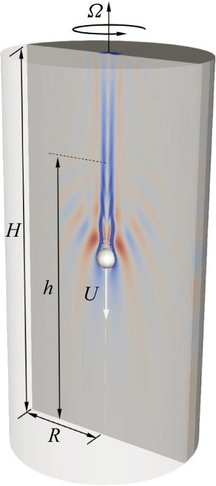
A circular cylinder of radius
 $R$
and height
 $H$
, filled with a fluid of kinematic viscosity
 $\nu$
and density
 $\rho$
, rotates about its axis at a constant angular rate
 $\varOmega$
. A small sphere of radius
 $a$
, co-rotating with the cylinder, is placed on the axis at distance
 $h$
from the bottom of the cylinder. The sphere impulsively starts to travel down the axis at a constant speed
 $U$
until it reaches the bottom endwall and then remains static. Figure 1 shows a schematic of the flow.
The ratios of the cylinder radius and height to the radius of the sphere are
 \begin{equation} a_R={R}/{a} \quad \textrm {and}\quad a_H={H}/{a}. \end{equation}
The ratio of the rotation time scale,
 $\tau _\varOmega =1/\varOmega$
, and the sphere translation time scale,
 $\tau _U=a/U$
, gives the Rossby number:
 \begin{equation} \textit{Ro}=\frac {U}{a\varOmega }. \end{equation}
The ratio of the viscous time scale based on the sphere’s radius,
 $\tau _\nu =a^2/\nu$
, and the rotation time scale,
 $\tau _\varOmega$
, gives the Taylor number:
 \begin{equation} \textit{Ta}=\frac {a^2\varOmega }{\nu }. \end{equation}
The Reynolds number, the ratio of
 $\tau _\nu$
and
 $\tau _\varOmega$
,
 \begin{equation} \textit{Re} = \textit{RoTa} = \frac {aU}{\nu }, \end{equation}
is also used to characterise these flows.
Schematic of the flow set-up, showing the sphere of radius
 $a$
travelling down the axis at constant speed
 $U$
and contours of the azimuthal vorticity
 $\eta$
for
 $\textit{Ta}=300$
and
 $\textit{Ro}=0.834$
at some time after the sphere was released a distance
 $h$
from the bottom endwall.

Using
 $a$
as the length scale,
 $a/U$
as the time scale, so that
 $U$
is the velocity scale, and
 $\rho a \varOmega U$
as the pressure scale, the non-dimensional Navier–Stokes equations in the rotating reference frame are
 \begin{equation} \textit{Ro}\left [ {\boldsymbol u}_t + (\boldsymbol{u \boldsymbol{\cdot }\boldsymbol{\nabla }}) \boldsymbol{u}\right ] = -\boldsymbol{\nabla }\! p -2{\boldsymbol e}_z \times \boldsymbol{u} +\frac {1}{Ta}{\nabla} ^2\boldsymbol{u}, \quad \boldsymbol{\nabla \boldsymbol{\cdot }u} = 0, \end{equation}
where
 $p$
is the reduced pressure incorporating the centrifugal term,
 $\boldsymbol{u}=(u,v,w)$
is the velocity in cylindrical coordinates
 ${\boldsymbol r}=(r,\theta ,z) \in [0,a_R]\times [0,2\pi ]\times [0, a_H]$
and
 ${\boldsymbol e}_z$
is the unit vector in the axial direction
 $z$
.
The velocity boundary conditions are no slip, i.e.
 ${\boldsymbol u}={\boldsymbol 0}$
on the cylinder walls and the surface of the sphere, except for the axial component of
 $\boldsymbol u$
on the sphere which is
 $w=-1$
for
 $0\leqslant t\lt z_0$
(prior to impact) and
 $w=0$
for
 $t \geqslant z_0$
(perfect inelastic collision). The axial location from which the sphere is released at
 $t=0$
is denoted
 $z_0=h/a$
.
Formally taking the limit
 $\textit{Ro}\to 0$
allows for the study of the quasi-steady linear dynamics (Tanzosh & Stone Reference Tanzosh and Stone1994; Bush et al. Reference Bush, Stone and Bloxham1995; Ungarish Reference Ungarish1996). This linearisation is quite different from simply taking
 $(\boldsymbol{u \boldsymbol{\cdot }\boldsymbol{\nabla }}) \boldsymbol{u}={\boldsymbol 0}$
whilst retaining
 ${\boldsymbol u}_t$
. We also solve such an unsteady linear system and compare with the corresponding nonlinear system to highlight the regions where nonlinear effects are small or large over wide ranges of
 $\textit{Ro}$
and
 $\textit{Ta}$
.
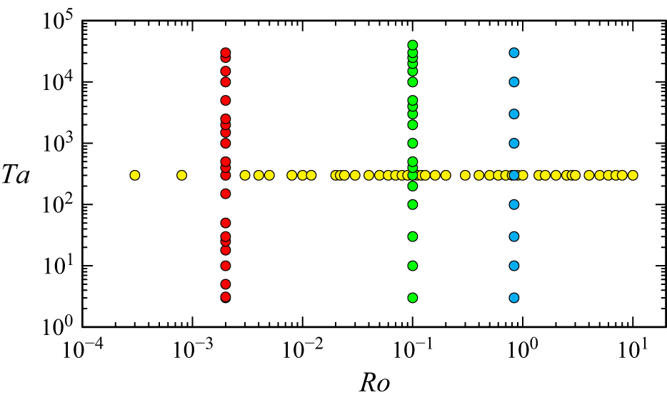
Loci in
 $(\textit{Ro},\textit{Ta})$
parameter space of the cases simulated in this study.

We use the same geometry as in the experiments of Pritchard (Reference Pritchard1969), whose cylinder had radius
 $R={15.24}\,\textrm {cm}$
and length
 $H={60.96}\,\textrm {cm}$
and the sphere had radius
 $a={1.5875}\,\textrm {cm}$
. This corresponds to
 $a_R=9.6$
and
 $a_H=38.4$
. In the experiments, the sphere co-rotating with the cylinder was released from
 $z_0=30$
and towed at a constant speed; our simulations also enforce these conditions. All the experiments were reported to have
 $\textit{Re}\gtrsim 250$
and
 $\textit{Ro} \in [0.1,2]$
. However, the individual results did not specify exact values of these parameters. Considering experiment B of Pritchard (Reference Pritchard1969) with
 $\textit{Ro}=0.834$
and assuming
 $\textit{Re}=250$
suggests that
 $\textit{Ta}=300$
. For
 $\textit{Ta}=300$
we consider a detailed sweep in Rossby number, with
 ${3\times {10}^{-4}}\leqslant \textit{Ro}\leqslant 10$
and for a few values of
 $\textit{Ro}$
we consider detailed sweeps with
 $3\leqslant Ta\leqslant {3\times 10^4}$
; the parameter sweeps are illustrated in figure 2.
In this study, we restrict our attention to axisymmetric flows, for which it is convenient to present the solutions in terms of a streamfunction
 $\psi$
, angular momentum
 $\gamma$
and azimuthal component of vorticity
 $\eta$
, where the velocity and vorticity in the rotating reference frame are
 \begin{equation} {\boldsymbol u}=(u,v,w)=\frac {1}{r}(-\psi _z, \gamma , \psi _r) \quad \textrm {and} \quad {\boldsymbol \omega }=(\xi ,\eta ,\zeta )=\frac {1}{r}(-\gamma _z, r\eta , \gamma _r), \end{equation}
where
 \begin{equation} \eta = u_z -w_r = -\frac {1}{r}\left(\psi _{zz} +\psi _{rr}-\frac {1}{r}\psi _r\right)\!. \end{equation}
The static frame velocity and vorticity are
 ${\boldsymbol u}+(0,r,0)$
and
 ${\boldsymbol \omega }+(0,0,2)$
. It is also convenient to introduce a streamfunction relative to the axially translating sphere,
 $\psi ^s=\psi +0.5r^2$
; this will facilitate comparisons with others who present their result in such a reference frame. Note that the pressure and the vorticity remain the same in the rotating cylinder frame and the rotating frame translating with the sphere.
2.1. Numerics
The governing equations (2.5) are discretised on a staggered grid with the velocity components at the faces and the pressure in the centre of the computational cells. The resulting system of equations is solved using a fractional-step method. The finite-difference solver is based on that described by Verzicco & Orlandi (Reference Verzicco and Orlandi1996) and has been tested in a wide variety of enclosed cylindrical flows (Verzicco & Camussi Reference Verzicco and Camussi1997; Verzicco et al. Reference Verzicco, Lalli and Campana1997; Pacheco et al. Reference Pacheco, Ruiz–Angulo, Zenit and Verzicco2011), establishing resolution requirements over a wide range of parameters. An immersed boundary method (Fadlun et al. Reference Fadlun, Verzicco, Orlandi and Mohd-Yusof2000) is used for the motion of the sphere, and solved with the governing equations using interpolations at every time step. Each time step is self-starting and thus the geometric conservation laws are preserved as long as the grid is frozen while computing the third-order Runge–Kutta steps. After these steps are completed, the velocity components and pressure quantities can be interpolated onto the new grid, guaranteeing conservation of volume or mass.
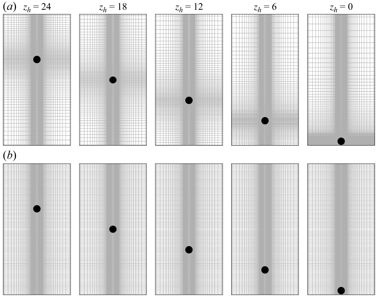
Snapshots of the moving grid (a), with
 $n_r\times n_z=151\times 351$
, and of the static axially uniform grid (b) with
 $n_r\times n_z=151\times 751$
(plotting only every fifth grid line for each set) at various times when the sphere is at axial location
 $z=z_h$
as indicated.

The same solver was used in a related study considering small axial oscillations of a sphere at the centre of a rotating cylinder (Pacheco et al. Reference Pacheco, Lopez and Verzicco2025). The grid is clustered about the sphere in the
 $r$
and
 $z$
directions, and since in that earlier study the sphere displacements were small, a static grid was used. In the current problem the sphere traverses along the axis and a moving grid that follows the sphere has been used. Snapshots of the moving grid as the sphere travels down the axis are illustrated in figure 3(a), while figure 3(b) shows an example of a static grid, uniformly distributed in the axial direction but with the same radial clustering as in the moving grid. A sequence of such static grids with increasing resolution is used to test the accuracy and efficiency of using the moving grid. The moving grid with axial clustering about the sphere maintains high spatial resolution in the vicinity of the sphere, necessary for resolving the thin boundary layers, while avoiding unnecessary refinement in the far field. This approach enhances the standard immersed boundary method by coupling it with a body-following grid, similar to overset techniques, but without the computational overhead of generating separate foreground and background grids. Note that this methodology necessitates the interpolation of flow variables at each grid movement step.
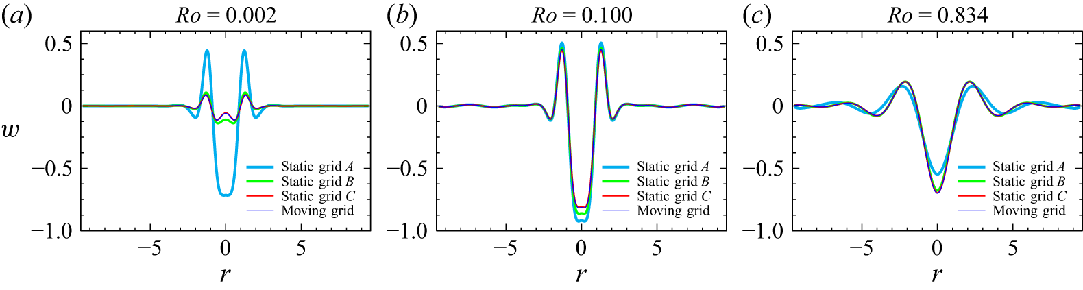
Radial profiles of
 $w$
at
 $z=18$
and
 $t=12$
with the sphere initially at
 $z=30$
for
 $\textit{Ta}=300$
and (a–c)
 $\textit{Ro}$
as indicated, computed using the moving grid with
 $n_r\times n_z=151\times 351$
and three static grids with
 $n_r=151$
and
 $n_z=551$
, 651 and 751 for grids
 $A$
,
 $B$
and
 $C$
, respectively.

To verify solution accuracy with respect to both the grid motion and density, results from the
 $n_r\times n_z=151\times 351$
moving grid are compared against three static grids, denoted
 $A$
,
 $B$
and
 $C$
, all with
 $n_r=151$
and
 $n_z=551$
, 651 and 751, respectively. Figure 4 demonstrates the convergence of the solutions, using radial profiles of the axial velocity
 $w$
at
 $z=18$
and
 $t=12$
with the sphere initially at
 $z=30$
for
 $\textit{Ta}=300$
and three representative Rossby numbers,
 $\textit{Ro}=0.002$
,
 $0.100$
and
 $0.834$
. All simulations maintained a Courant–Friedrichs–Lewy condition of
 $1$
with a maximum time step of
 $\delta _t=0.0005$
. The results confirm that static grid solutions converge as
 $n_z\to 751$
to the moving grid solution with
 $n_z=351$
. The moving grid maintains a high resolution clustered around the sphere and yields results equivalent to those of much finer axial grids at a significantly lower computational cost. This efficiency facilitates the extensive parametric studies conducted in this work.
As part of the flow diagnostics, displacements of passive tracers were tracked over the flow evolution. The tracers were initially placed on horizontal lines extending from the axis to the cylinder sidewall at various axial locations. Their subsequent positions
 $(r_p,z_p)$
were determined by solving
 $(\dot {r}_p,\dot {z}_p)=(u,w)$
using the velocities at the cells surrounding the position of each particle interpolated (using a three-point upstream-weighted quadratic spatial interpolation) to the particle position using a third-order Runge–Kutta (RK3) method consistent with the overall time-integration scheme of the Navier–Stokes solver.
3. Results
3.1. Pritchard’s experiment
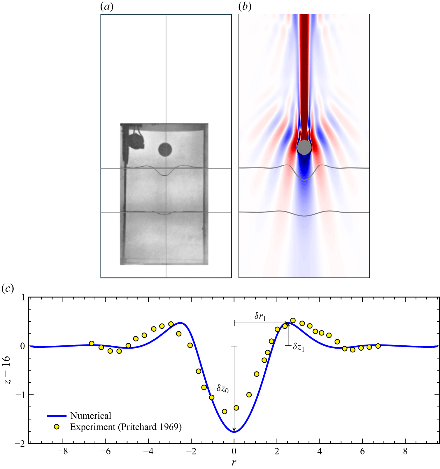
We begin by simulating the flow corresponding to experiment B from Pritchard (Reference Pritchard1969), described in § 2. In that experiment, a pair of thin platinum wires were stretched orthogonal to the cylinder axis, at axial locations
 $z=16$
and
 $10$
, well below the location
 $z=z_0=30$
from where the sphere begun its traverse down the axis. The water contained Thymol Blue, and when a small voltage was applied across the wires, dyelines were produced. These were displaced as the travelling sphere approached them. A snapshot of the experiment at non-dimensional time
 $t=12$
is reproduced in figure 5
 $(a)$
, where the cropped experimental image is placed within the outline of the whole cylinder. Figure 5
 $(b)$
shows a snapshot from our numerical simulation at the same time for the parameters corresponding to the experiment, showing contours of the axial component of vorticity
 $\zeta$
and the distorted numerical dyelines. Figure 5
 $(c)$
compares at
 $t=12$
the numerical dyeline (blue) that was initially a straight line at
 $z=16$
with the experimental results (yellow symbols), determined using measurements from the photograph shown in figure 5
 $(a)$
. The agreement is very reasonable, considering how sensitive dye transport is to small imperfections in initial position in unsteady flows (Lopez & Perry Reference Lopez and Perry1992). The shape of the distorted dyeline has much in common with the radial profile of the axial velocity ahead of a translating body in a linear inviscid setting (Morgan Reference Morgan1951, figure 3), and it is also very similar to the hydrogen bubble distributions ahead of the sphere shown in Maxworthy (Reference Maxworthy1970, figure 14), whose experiment corresponded to
 $\textit{Ta}=83$
,
 $\textit{Ro}\sim 1$
,
 $a_H=156$
and
 $a_R=15.6$
. We characterise the dyeline distortion by
 $\delta z_0$
, the axial distance the dye is displaced on the axis, and the displacement in the axial direction
 $\delta z_1$
at the radial location
 $\delta r_1$
of the maximum off-axis displacement, at time
 $t=12$
for the dyeline initially at
 $z=16$
; these displacements are indicated in figure 5
 $(c)$
.
 $(a)$
Flow visualisation of Pritchard (Reference Pritchard1969, experiment B, figure 2), with the cropped image placed inside the outlined rotating cylinder.
 $(b)$
Snapshot of the simulated axial vorticity
 $\zeta$
at
 $t=12$
with
 $z=30$
,
 $\textit{Ro}=0.834$
and
 $\textit{Ta}=300$
(corresponding to the experimental parameters).
 $(c)$
Comparison between our numerical result and the experiment of Pritchard (Reference Pritchard1969) of the displacement of passive tracers due to the motion of the sphere. At
 $t=0$
, the experimental dye and the numerical tracers are flat at
 $z=16$
. The dye displacement on the axis
 $\delta z_0$
and the displacement in the axial direction
 $\delta z_1$
at the radial location
 $\delta r_1$
of the maximum off-axis displacement are indicated.

3.2.
Effects of varying
 $\textit{Ro}$
at
$\textit{Ta}=300$


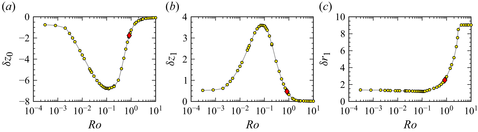
Figure 6 summarises how the upstream influence depends on
 $\textit{Ro}$
for
 $\textit{Ta}=300$
,
 $a_R=9.6$
and
 $a_H=38.4$
(corresponding to experiment B of Pritchard (Reference Pritchard1969)), quantified by
 $\delta z_0$
,
 $\delta z_1$
and
 $\delta r_1$
at
 $t=12$
for dyelines initially at
 $z=16$
. The most striking result is that the upstream influence is greatest at
 $\textit{Ro}\sim 0.1$
, and diminishes with increasing and decreasing
 $\textit{Ro}$
. The results indicate that as
 $\textit{Ro}\to 0$
, the dye axial displacement asymptotes to
 $\delta z_0\sim -0.7$
and
 $\delta z_1\sim 0.5$
, which are small, but perhaps more significant is that
 $\delta r_1\to \sim 1.4$
, indicating that at small
 $\textit{Ro}$
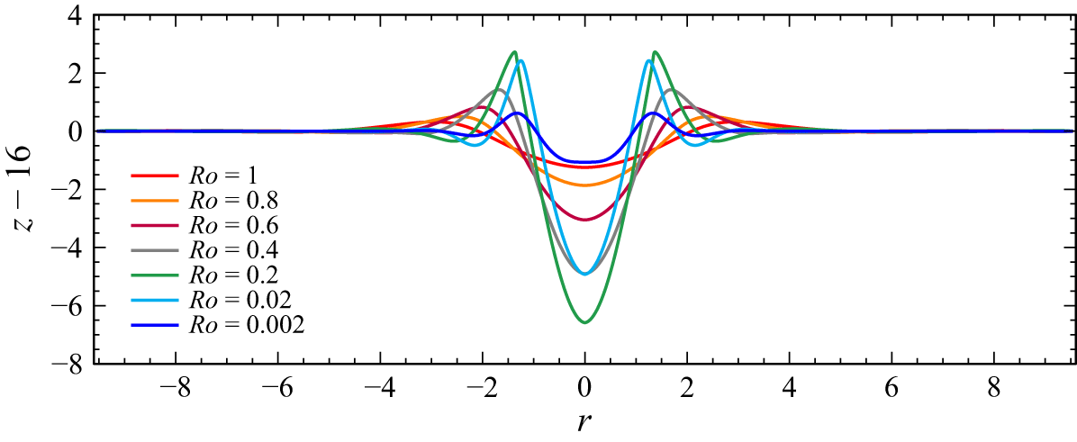
, upstream influence is associated with the Stewartson shear layer emitted in the axial direction (both fore and aft) from the equator of the slowly translating sphere. The dyelines are shown in figure 7 for a selection of
 $\textit{Ro}$
values. For
 $\textit{Ro}$
increasing beyond
 $\sim \kern-1pt 2$
, there is a rapid transition with
 $\delta z_0\to 0$
,
 $\delta z_1\to 0$
and
 $\delta r_1\to a_H$
, indicating no upstream influence. For
 $\textit{Ro}\gtrsim 2$
, the effects of background rotation are greatly diminished and the flow is essentially the same as that of the non-rotating
 $\textit{Ro}\to \infty$
situation, considered in detail in Pacheco et al. (Reference Pacheco, Ruiz–Angulo, Zenit and Verzicco2011).
Variation with
 $\textit{Ro}$
of the displacement
 $\delta z_0$
of dye, initially at
 $z=16$
, in the axial direction at the axis, and the displacement in the axial direction
 $\delta z_1$
at the radial location
 $\delta r_1$
of the maximum off-axis displacement, for
 $\textit{Ta}=300$
at
 $t=12$
. The red diamonds at
 $\textit{Ro}=0.834$
correspond to the
 $\textit{Ro}$
value in experiment B of Pritchard (Reference Pritchard1969).

Numerical dyelines, initially flat at
 $z=16$
, shown at
 $t=12$
for
 $\textit{Ta}=300$
and
 $\textit{Ro}$
as indicated.

Snapshots of the azimuthal vorticity
 $\eta$
at
 $t=12$
, for
 $\textit{Ta}=300$
and
 $\textit{Ro}$
as indicated. The initial axial positions of the tracers are
 $z=4$
,
 $9.6$
,
 $16$
,
 $24$
,
 $28$
and
 $32.5$
. Supplementary movie 1 animates these from
 $t=0$
to
 $t=35$
. The animations also include a view in the reference frame translating with the sphere.

Figure 8. Long description
A series of heat maps showing azimuthal vorticity around a sphere at different Rossby numbers. Each heat map represents a snapshot of the vorticity field at a specific Rossby number, ranging from 0.002 to 2.0. The heat maps are arranged in a grid layout with two rows and four columns. Each heat map shows the distribution of vorticity around a central sphere, with color intensity indicating the magnitude of vorticity. The color scale ranges from blue, indicating lower vorticity, to red, indicating higher vorticity. The Rossby numbers are labeled above each heat map. The heat maps show the evolution of vorticity patterns as the Rossby number increases, with more complex and intense vorticity structures appearing at higher Rossby numbers.
Figure 8 shows snapshots of the azimuthal vorticity
 $\eta$
at
 $t=12$
, for a selection of
 $\textit{Ro}$
from the cases in figure 6. Supplementary movie 1 available at https://doi.org/10.1017/jfm.2026.11927 animates these from
 $t=0$
to
 $t=35$
, showing how the dye is displaced over time. The figure and the movie include several additional dyelines in order to provide additional information on how they are displaced as the sphere approaches them and translates past their original positions. The movie also includes a windowed view of
 $\eta$
as seen by an observer moving with the sphere. In this view, it is clear that after a short transient (which grows longer with increasing
 $\textit{Ro}$
), the flow relative to the translating sphere is essentially steady within several radii of the sphere, until it comes close to the bottom endwall (this distance to the bottom increases with
 $\textit{Ro}$
). For all
 $\textit{Ro}$
considered, the animations show that
 $t=12$
is roughly when the start-up transients have diminished and the unsteadiness due to the approach to the bottom is small; this is very likely why Pritchard (Reference Pritchard1969) chose this time to take snapshots of the experimental flow. At this time, the sphere is approximately half-way between the top and bottom of the cylinder (the sphere is at
 $z=18$
while the centre of the cylinder is at
 $z=a_H/2=19.2$
). The time when an axially translating body is at the mid-way location is when Ungarish (Reference Ungarish1996, Reference Ungarish2024) conducts steady-state analyses of the flows.
Snapshots at time
 $t=12$
for
 $\textit{Ta}=300$
and
 $\textit{Ro}$
as indicated of the axial vorticity
 $\zeta$
, the azimuthal vorticity
 $\eta$
, the reduced pressure
 $p$
, the instantaneous streamfunction
 $\psi$
and the instantaneous streamfunction relative to the travelling sphere
 $\psi ^s=\psi +0.5r^2$
(uniformly spaced contour levels with
 $\psi ^s\in [0,50]$
).

Figure 9 considers three cases at
 $\textit{Ta}=300$
. One is the weakly nonlinear case with
 $\textit{Ro}=0.002$
, the second is
 $\textit{Ro}=0.100$
which has maximal upstream influence (using displacement at
 $t=12$
of the dyeline at
 $z=16$
as a metric) and the third is
 $\textit{Ro}=0.834$
corresponding to Pritchard’s experiment B. The figure shows snapshots at
 $t=12$
of the axial vorticity
 $\zeta$
, the azimuthal vorticity
 $\eta$
, the reduced pressure
 $p$
, the instantaneous streamfunction
 $\psi$
and the instantaneous streamfunction relative to the travelling sphere
 $\psi ^s=\psi +0.5r^2$
. For
 $\textit{Ro}=0.002$
at this time with the sphere close to the centre of the cylinder, the flow close to the sphere is essentially steady relative to the moving sphere, except in the viscous boundary layer which oscillates at this
 $\textit{Ta}$
(as is evident in supplementary movie 1). The flow is very nearly fore–aft symmetric about the equator of the sphere at this time, with
 $\zeta$
and
 $p$
anti-symmetric in
 $z$
while
 $\eta$
and the two streamfunctions are symmetric in
 $z$
. The anti-symmetry in
 $\zeta$
corresponds to the vortex lines in the column ahead of the travelling sphere being compressed as the distance to the upstream endwall is reduced, resulting in the observed negative relative axial vorticity, while in the wake the distance between the aft endwall and the sphere is increasing, stretching the vortex lines and producing positive relative axial vorticity. This is in accord with the theoretical analysis of confinement effects in Moore & Saffman (Reference Moore and Saffman1968). Outside of the Taylor column (
 $r\gtrsim \delta r_1\sim 1.5$
), the flow is essentially in solid-body rotation (
 $\boldsymbol{u}\approx 0$
and
 $\boldsymbol{\omega }\approx 0$
); Moore & Saffman (Reference Moore and Saffman1968) refer to the flow in this outer region as geostrophic. The instantaneous streamlines in the cylinder frame,
 $\psi$
, indicate that the instantaneous flow ahead of the sphere from the sphere’s forward polar region is directed down the axis, slows down as it approaches the upstream endwall and turns around, returning to the equatorial region of the sphere which it passes towards the aft endwall, slows down and turns back towards the rear polar region of the sphere. Surrounding this columnar region of flow associated with the negative (blue) streamlines just described is a sheath of positive (red) streamlines with counter meridional flow. The streamlines relative to the translating sphere
 $\psi ^s$
instead are everywhere positive for this small
 $\textit{Ro}$
, indicative of the nearly uniform axial flow past the sphere which slows down as it is diverted around the sphere and then is accelerated past it.
The flow at
 $\textit{Ro}=0.100$
(second row of figure 9) has similar features to the lower-
 $\textit{Ro}$
flow described above, but the fore–aft symmetry is more strongly broken. This asymmetry is evidenced by the formation of an inertial wave pattern emitted upstream from the back end of the sphere. The usual linear inviscid dispersion relation for inertial waves (Greenspan Reference Greenspan1968) needs to be corrected by a Doppler shift due to the travelling source, i.e. the translating sphere (Taylor Reference Taylor1922; Lighthill Reference Lighthill1967; Aurégan et al. Reference Aurégan, Bonometti and Magnaudet2023). This pattern of standing waves moves steadily with the sphere (see supplementary movie 1) and fans out radially with increasing
 $\textit{Ro}$
(as can be appreciated in figure 8 illustrating this effect for various
 $\textit{Ro}$
).
By
 $\textit{Ro}=0.834$
(third row of figure 9), the inertial wave pattern fills a considerable portion of the entire cylinder, so that the region outside the Taylor column is no longer in solid-body rotation. The streamfunction
 $\psi$
is largest in the upstream region (bottom half of the cylinder) and correlates very well with the azimuthal vorticity. On the other hand, the streamlines relative to the sphere,
 $\psi ^s$
, only exhibit waviness aft of the sphere. Similar flow features of the streamlines in the cylinder and the sphere frames of reference were reported by Wang et al. (Reference Wang, Lu and Zhang2004), who simulated the flow past a sphere in a rotating pipe with steady uniform axial and angular velocity upstream of the sphere.
The waviness in
 $\psi ^s$
being only present aft of the sphere for the larger
 $\textit{Ro}$
is a flow feature much like that in the dye images of Long (Reference Long1953), on which the hypothesis of no upstream influence was based for
 $\textit{Ro}\gtrsim 0.2$
. Those experiments were conducted in a rotating cylinder of radius
 $R={29}\,\textrm {cm}$
, height
 $H={90}\,\textrm {cm}$
and rotating at
 $\varOmega ={1.047}\,\rm {rad\,s}^{-1}$
. The axisymmetric body consisted of a leading hemisphere of radius
 $a={3.8}\,\textrm {cm}$
with a trailing tapered cone having total length
 $2.95a$
; the purpose of the tapering was to minimise effects of boundary-layer separation. Using the radius of the body, the experiments correspond to
 $a_R=7.3$
and
 $a_H=23.7$
, so potentially suffered more radial and axial confinement effects than in Pritchard’s experiments. It was not explicitly stated, but it seems that the body was towed at constant speeds corresponding to
 $\textit{Ro}\in [0.16,0.34]$
. Assuming
 $\nu ={0.01}{\,\textrm {cm}^2\,\textrm {s}^{-1}}$
(the experiments used water, but the temperature was not specified) gives a Taylor number
 $\textit{Ta}={1.5\times 10^3}$
. The experiments used dye flow visualisation (the dye was produced by a dissolving pellet of potassium permanganate that was dropped into the cylinder just before the body started to translate along the axis), that displayed waviness near the translating body and decaying in the outer aft wake. No waviness in the dye was evident ahead of the body, leading to the hypothesis of no upstream influence. But these unsteady dye visualisations are very difficult to interpret, even beyond their erratic behaviour due to the pellets being dropped. Long’s dye streaks resemble the wavy instantaneous streamfunction relative to the translating sphere
 $\psi ^s$
which has no waviness ahead of the sphere, rather than
 $\psi$
. The structure of
 $\psi$
correlates very well with that of
 $\eta$
, which is the same in the two reference frames, and does indicate a strong upstream influence.
Variation with
 $\textit{Ro}$
of the wavelength
 $\varLambda$
of the emitted inertial waves at
 $t=12$
for
 $\textit{Ta}=300$
, determined using the azimuthal vorticity,
 $\varLambda _\eta$
, and the pressure,
 $\varLambda _p$
.

The pressure and vorticity are the same in the rotating frame with the sphere translating and in the rotating frame translating with the sphere. For
 $0.1\lesssim Ro\lesssim 2$
, the inertial wave pattern emitted upstream from the back end of the sphere has a wavelength
 $\varLambda$
that varies with
 $\textit{Ro}$
. Taylor (Reference Taylor1922) estimated this wavelength from the steady inviscid equations and accounting for the Doppler shift in their frequency due to the moving sphere in an unbounded rotating ambient to be
 $\varLambda =\pi \textit{Ro}$
. Aurégan et al. (Reference Aurégan, Bonometti and Magnaudet2023) estimated the wavelength in their system determined by the minimum distance separating two successive crests in the pressure at steady state. At
 $t=12$
, we also use this method to obtain the wavelength based on the pressure,
 $\varLambda _p$
, as well as the azimuthal vorticity taking
 $\varLambda _{\eta }$
to be the distance between the extrema in the first and second bands of negative
 $\eta$
emitted from the sphere (compare the snapshots of
 $\eta$
and
 $p$
for
 $\textit{Ro}=0.834$
in figure 9). Figure 10 shows how
 $\varLambda _\eta$
and
 $\varLambda _p$
vary with
 $\textit{Ro}$
for
 $\textit{Ta}=300$
at
 $t=12$
. The two measures of
 $\varLambda$
agree fairly well given the numerical difficulties in determining the positions of the extrema in variables that vary slowly along the bands. The figure includes a (blue) line corresponding to Taylor’s estimate; this does not agree with our data, except perhaps as
 $\textit{Ro}\to 0$
where
 $\varLambda$
appears to vary linearly with
 $\textit{Ro}$
. Another (red) line corresponding to the fit
 $\varLambda =2\pi \textit{Ro}^2$
better captures our data for
 $\textit{Ro}\gtrsim 0.4$
; this is simply an ‘eyeball’ fit to the data. The discrepancy with Taylor’s estimate is most likely due to our flow being confined inside a cylinder with the sphere travelling along the axis. Aurégan et al. (Reference Aurégan, Bonometti and Magnaudet2023) find good agreement between their wavelength measurements and Taylor’s estimate; this is most likely due to both considering a uniform flow past a stationary sphere at steady state.
As noted earlier, the regions of negative and positive instantaneous streamlines
 $\psi$
correlate quite well with the regions of negative and positive azimuthal vorticity
 $\eta$
. If the flow was steady and inviscid, and well upstream of the sphere the flow had uniform axial and angular velocity components, then
 $\psi ^s$
would satisfy a linear equation (Long Reference Long1953; Stewartson Reference Stewartson1968; Benjamin Reference Benjamin1970; Stewartson Reference Stewartson1970):
 \begin{equation} \psi ^s_{zz}+\psi ^s_{rr}-r^{-1}\psi ^s_r+4\textit{Ro}^{-2}\psi ^s=F(r), \end{equation}
where
 $F(r)$
is an arbitrary function determined by boundary and/or far-field conditions. Attempts to reconcile this with physical arguments and experimental observation led Benjamin (Reference Benjamin1970) and Stewartson (Reference Stewartson1970) to question the underlying assumptions necessary for the no upstream hypothesis of Long (Reference Long1953), namely that the flow is steady and inviscid with uniform axial and angular velocity components far upstream. The upstream conditions are by definition not applicable to the axially confined case considered here. Further, note that for the flows we consider, we have
 \begin{equation} \psi ^s_{zz}+\psi ^s_{rr}-r^{-1}\psi ^s_r=\psi _{zz}+\psi _{rr}-r^{-1}\psi _r=-r\eta . \end{equation}
It is unclear how all of this is inter-related as all attempts to tie down a form for
 $F(r)$
whilst retaining the underlying assumptions that introduce it have failed. Relaxing the steady inviscid flow idealisations introduces
 $\textit{Ta}$
effects in the flows, which we consider in the following subsection.
3.3.
Effects of varying
$\textit{Ta}$

For the three representative Rossby numbers used in the previous subsection,
 $\textit{Ro}=0.002$
,
 $0.100$
and
 $0.834$
, we now consider how the flows at these
 $\textit{Ro}$
vary with
 $\textit{Ta}$
. Figure 11 shows the flow-distorted numerical dyelines at
 $t=12$
, which were initially horizontal at
 $z=16$
, for those
 $\textit{Ro}$
and various Taylor numbers ranging from
 $\textit{Ta}=3$
to
 $3\times 10^4$
. For the largest
 $\textit{Ro}=0.834$
, there is a smooth and mild variation in the dyelines with
 $\textit{Ta}$
, but for the two smaller
 $\textit{Ro}$
, there is a qualitative change in behaviour at
 $\textit{Ta}\sim 300$
. For smaller
 $\textit{Ta}$
, the dyelines are qualitatively the same as at
 $\textit{Ta}=300$
, with a large upstream displacement of the dye on the axis and a relatively smaller deflection back towards the sphere at a radial distance a little beyond the radius of the sphere.
Numerical dyelines, initially flat at
 $z=16$
, shown at
 $t=12$
for
 $\textit{Ro}$
and
 $\textit{Ta}$
as indicated.

Figure 11. Long description
Three line graphs depict the effects of axial confinement on fluid dynamics. Panel A: The line graph shows the relationship between the radial position (r) and the axial vorticity at a fixed depth (z = -16) for a Rossby number (Ro) of 0.002. The graph includes multiple lines representing different Taylor numbers (Ta = 3, 30, 300, 3000, 30000). The lines exhibit varying patterns of axial vorticity, with notable peaks and troughs around the center (r = 0). Panel B: The line graph illustrates the same relationship for a Rossby number (Ro) of 0.100. The patterns are more pronounced with higher peaks and deeper troughs compared to Panel A. Panel C: The line graph shows the relationship for a Rossby number (Ro) of 0.834. The lines are smoother with less pronounced peaks and troughs, indicating a different dynamic behavior at higher Rossby numbers. Each graph includes a legend indicating the Taylor numbers and their corresponding lines.
For both
 $\textit{Ro}=0.100$
and
 $0.002$
, we see that for
 $\textit{Ta}\gtrsim 300$
the dyeline distortions show large radial oscillations within
 $r\lesssim 1$
. This is consistent with the speculative ideas put forward by Pritchard (Reference Pritchard1969). In his figure 15, Pritchard presents sketches of conjectured flow patterns for various
 $\textit{Ro}$
ranges that follow what our simulations reveal. However, he does not indicate the ranges of
 $\textit{Ta}$
that these are for and he notes that his experimental apparatus could not be used at low values of
 $\textit{Ro}$
.
Variation with
 $\textit{Ta}$
of the displacement
 $\delta z_0$
of dye, initially at
 $z=16$
, in the axial direction at the axis, and the displacement in the axial direction
 $\delta z_1$
at the radial location
 $\delta r_1$
of the maximum off-axis displacement, at
 $t=12$
and for
 $\textit{Ro}$
as indicated.

As was done earlier for
 $\textit{Ta}=300$
, we characterise the dyeline distortions using
 $\delta z_0$
,
 $\delta z_1$
and
 $\delta r_1$
(see figure 5). These are summarised in figure 12. For
 $\textit{Ro}=0.834$
, the dyeline displacements are essentially independent of
 $\textit{Ta}$
for
 $\textit{Ta}\gtrsim {10^2}$
, so that even though Pritchard does not state precisely the value of
 $\textit{Ta}$
for his experiment B, this is not a major problem. For the two smaller
 $\textit{Ro}$
values,
 $\delta r_1 \to 1$
with increasing
 $\textit{Ta}$
, with the maximal off-axis displacement
 $\delta z_1$
growing with
 $\textit{Ta}$
and this grows fastest for
 $\textit{Ro}=0.100$
. For
 $\textit{Ro}=0.100$
this indicates that the dye well upstream of the sphere is sucked up and pushed back towards the aft wake through the thin Stewartson layer at
 $r\approx 1$
. At time
 $t=12$
, the sphere is at
 $z=18$
which is one sphere diameter above the initial location of the dyeline at
 $z=16$
; for flows with
 $\delta z_1\gt 2$
some of the dyeline has been advected back past the equator of the sphere. Figure 12
 $(b)$
indicates that for
 $\textit{Ro}=0.002$
and
 $\textit{Ro}=0.100$
this happens for
 $\textit{Ta}\gtrsim 100$
, but for
 $\textit{Ro}=0.834$
this does not occur for any
 $\textit{Ta}$
.
Snapshots at time
 $t=12$
for
 $\textit{Ro}=0.002$
and
 $\textit{Ta}$
as indicated of
 $(a)$
 $\eta$
,
 $\eta _0$
and their difference and of
 $(b)$
 $2v$
,
 $\partial p/\partial r$
and their difference. Supplementary movie 2 animates
 $\eta$
from
 $t=0$
to
 $t=35$
, in both the cylinder frame and a windowed frame moving with the sphere.

Figure 13. Long description
The image contains multiple panels of graphs depicting the motion of a small body moving along the axis of a rotating fluid. Each panel shows different parameters and their differences over time. Panel A: This panel contains three rows of graphs. The first row shows the parameter η for different values of Ta (3, 30, 300, 3000, and 30000). The second row shows the parameter η0 for the same values of Ta. The third row shows the difference between η and η0 for the same values of Ta. Each graph has a vertical axis labeled with the parameter and a horizontal axis labeled with the position along the axis of rotation. The color scale at the bottom indicates the range of values from -2 to 2. Panel B: This panel also contains three rows of graphs. The first row shows the parameter 2v for different values of Ta. The second row shows the parameter ∂p/∂r for the same values of Ta. The third row shows the difference between 2v and ∂p/∂r for the same values of Ta. Each graph has a vertical axis labeled with the parameter and a horizontal axis labeled with the position along the axis of rotation. The color scale at the bottom indicates the range of values from -2 to 2. The graphs show the evolution of these parameters over time and their differences, providing insights into the fluid dynamics of the system.
Snapshots at time
 $t=12$
for
 $\textit{Ro}=0.100$
and
 $\textit{Ta}$
as indicated of
 $(a)$
 $\eta$
,
 $\eta _0$
and their difference and of
 $(b)$
 $2v$
,
 $\partial p/\partial r$
and their difference. Supplementary movie 3 animates
 $\eta$
from
 $t=0$
to
 $t=30.8$
, in both the cylinder frame and a windowed frame moving with the sphere.

Snapshots at time
 $t=12$
for
 $\textit{Ro}=0.834$
and
 $\textit{Ta}$
as indicated of
 $(a)$
 $\eta$
,
 $\eta _0$
and their difference and of
 $(b)$
 $2v$
,
 $\partial p/\partial r$
and their difference. Supplementary movie 4 animates
 $\eta$
from
 $t=0$
to
 $t=30.8$
, in both the cylinder frame and a windowed frame moving with the sphere.

Figure 15. Long description
Panel A: This panel contains three rows of heat maps. The first row shows the parameter eta for different values of Ta (3, 30, 300, 3000, 30000). The second row shows the parameter eta0 for the same values of Ta. The third row shows the difference between eta and eta0 for the same values of Ta. Each heat map uses a color scale ranging from -2 to 2, with blue indicating lower values and red indicating higher values. The heat maps show the formation and evolution of Taylor columns ahead of and behind the moving body. Panel B: This panel contains three rows of heat maps. The first row shows the parameter 2v for different values of Ta (3, 30, 300, 3000, 30000). The second row shows the parameter partial derivative p/partial derivative r for the same values of Ta. The third row shows the difference between 2v and partial derivative p/partial derivative r for the same values of Ta. Each heat map uses a color scale ranging from -2 to 2, with blue indicating lower values and red indicating higher values. The heat maps show the distribution and changes in velocity and pressure gradients around the moving body.
Supplementary movie 2 animates the azimuthal vorticity
 $\eta$
from
 $t=0$
to
 $t=35$
, in both the cylinder frame and a windowed frame moving with the sphere, for
 $\textit{Ro}=0.002$
and
 $\textit{Ta}=3$
,
 $30$
,
 $300$
,
 $3\times {10}^3$
and
 $3\times 10^4$
. As in supplementary movie 1, it shows how dyelines at various axial locations are distorted as the sphere traverses down the axis. For the smallest
 $\textit{Ta}=3$
and
 $30$
, the movie shows that
 $\eta$
quickly becomes steady relative to the moving sphere until the sphere is within a few radii of the bottom endwall. With increasing
 $\textit{Ta}$
, the
 $\eta$
distribution sharpens into a Stewartson layer distribution, and this structure is steady relative to the sphere until the sphere is close to the bottom endwall. However, as was noted earlier for
 $\textit{Ta}=300$
, the boundary layer on the sphere has temporal and spatial oscillations throughout the entire trajectory of the sphere. By
 $\textit{Ta}={3\times 10^3}$
these oscillations extend several sphere radii both upstream and downstream of the sphere and their radial extents fill the entire column
 $0\lt r\lt 1$
. These oscillations are responsible for the more complicated dyeline distortions noted earlier. At
 $\textit{Ta}={3\times 10^4}$
the amplitudes of these oscillations are sufficiently large that they cause inertial oscillations throughout the entire cylinder.
The first row of figure 13
 $(a)$
shows snapshots from supplementary movie 2 at
 $t=12$
. That figure also shows snapshots at the same time of the azimuthal vorticity
 $\eta _0$
computed at the same
 $\textit{Ro}$
and
 $\textit{Ta}$
but formally setting
 $(\boldsymbol{u \boldsymbol{\cdot }\boldsymbol{\nabla }}) \boldsymbol{u}={\boldsymbol 0}$
in (2.5). In this linear unsteady problem, the vortex line bending term
 $r^{-1}\partial v^2/\partial z$
is absent. In axisymmetric rotating flows with walls not having a component of motion in their normal directions, flows having any initial condition with
 $\eta =0$
only develop non-zero
 $\eta$
as a result of this vortex line bending term (Brown & Lopez Reference Brown and Lopez1990). In the flows under consideration, the translating sphere drives most of the azimuthal vorticity, especially for small
 $\textit{Ro}$
and
 $\textit{Ta}$
. The difference between
 $\eta$
and
 $\eta _0$
provides an indication of where the nonlinear advection terms are non-negligible. Perhaps surprisingly, the nonlinear
 $(\boldsymbol{u \boldsymbol{\cdot }\boldsymbol{\nabla }}) \boldsymbol{u}$
contributions are only significant at the very largest
 $\textit{Ta}={3\times 10^4}$
and the spatio-temporal oscillations are virtually indistinguishable between
 $\eta$
and
 $\eta _0$
for all
 $\textit{Ta}$
. Figure 13
 $(b)$
shows twice the azimuthal velocity
 $2v$
and the radial pressure gradient
 $\partial p/\partial r$
for the same flows as in figure 13
 $(a)$
. Geostrophic flow requires
 $2v=\partial p/\partial r$
, and the theoretical estimates of the drag on the sphere from Moore & Saffman (Reference Moore and Saffman1969) rely on
 $2v=\partial p/\partial r$
everywhere for large Taylor numbers (their equation (7.13)). This is not realised in the viscous boundary layer of the sphere (particularly for the smallest
 $\textit{Ta}$
) and inside the Taylor column for the larger
 $\textit{Ta}$
.
Figure 14 shows the same quantities as figure 13 but for
 $\textit{Ro}=0.100$
. The nonlinear and ageostrophic aspects of the flows are very evident for
 $\textit{Ta}\gtrsim 300$
and rapidly increase with increasing
 $\textit{Ta}$
. Supplementary movie 3 shows that the flow relative to the translating sphere quickly becomes steady for
 $\textit{Ta}\lesssim 300$
, with the start-up transients persisting longer for larger
 $\textit{Ta}$
, but the
 $\textit{Ta}={3\times 10^3}$
and
 $\textit{Ta}={3\times 10^4}$
flows relative to the sphere are never steady throughout the entire trajectory of the sphere. The oscillations are pronounced in the forward and aft Taylor column regions, with those in the aft being strongest, and these oscillations lead to inertial waves radiating throughout the cylinder. As the sphere approaches the bottom endwall, the oscillations in the aft wake intensify and emit a broad conical region of inertial waves backwards. These types of oscillations are present in both
 $\eta$
and
 $\eta _0$
, but their differences are of order one, so that nonlinearity influences them but is not necessary for their existence. The flows at
 $\textit{Ro}=0.002$
and
 $\textit{Ro}=0.100$
are very similar for
 $\textit{Ta}\lesssim 30$
, consistent with the dyeline deformation metrics reported in figure 12.
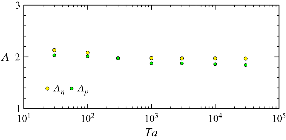
Variation with
 $\textit{Ta}$
of the wavelength
 $\varLambda$
of the emitted inertial waves at
 $t=12$
for
 $\textit{Ro}=0.834$
, determined using the azimuthal vorticity,
 $\varLambda _\eta$
, and the pressure,
 $\varLambda _p$
.

Figure 15 shows the same quantities as figures 13 and 14, but for
 $\textit{Ro}=0.834$
. The upstream influence at this larger
 $\textit{Ro}$
is due to the inertial waves rather than a Taylor column or Stewartson layers. The inertial waves are more intense with increasing
 $\textit{Ta}$
(or rather, with decreasing
 $\textit{Ta}$
they are viscously dissipated), but their wavelength is invariant with
 $\textit{Ta}$
for
 $\textit{Ta}\gtrsim 100$
; see figure 16. As with the
 $\textit{Ro}=0.100$
flows, the nonlinear contribution from
 $(\boldsymbol{u \boldsymbol{\cdot }\boldsymbol{\nabla }}){\boldsymbol u}$
increases with
 $\textit{Ta}$
, but this is primarily in the aft wake of the sphere. There are some nonlinear contributions in the inertial waves, but these quickly diminish upstream of the sphere, i.e. upstream of the sphere the inertial waves are essentially linear, even for the largest
 $\textit{Ta}={3\times 10^4}$
. The same is true for the ageostrophic aspects of the flows. Supplementary movie 4 animates
 $\eta$
from
 $t=0$
to
 $t=30.8$
, in both the cylinder frame and a windowed frame moving with the sphere, for the cases shown in figure 15. As with the
 $\textit{Ro}=0.100$
cases, the lowest
 $\textit{Ta}$
flows become steady relative to the sphere, but for
 $\textit{Ta}\gtrsim 300$
the flow relative to the sphere is never steady. However, the unsteadiness at
 $\textit{Ro}=0.834$
is considerably milder than for
 $\textit{Ro}=0.100$
at the same
 $\textit{Ta}$
values. A forward Taylor column with a Stewartson layer surrounding it never forms at
 $\textit{Ro}=0.834$
for any
 $\textit{Ta}$
considered; the more feeble upstream influence is due to the inertial wave pattern emitted to the fore of the sphere.
4. Discussion and conclusion
The numerical simulations have reproduced key features of Pritchard (Reference Pritchard1969) experiment B under similar geometric configurations and boundary conditions, showing quantitative agreement between simulated and experimental dyeline displacements despite the uncertainty in the experimental parameters and the sensitivity of dye transport in unsteady flows. The upstream influence, characterised by the formation of inertial waves, of a sphere translating along the axis of an enclosed rotating cylinder depends strongly on the Rossby number
 $\textit{Ro}$
. For the experimental value of the Taylor number,
 $\textit{Ta}=300$
, the upstream influence is maximal at
 $\textit{Ro} \approx 0.1$
and weakens for both smaller and larger
 $\textit{Ro}$
. At small
 $\textit{Ro}$
, the upstream effect is associated with a Taylor column bounded by Stewartson shear layers, while for
 $\textit{Ro}\gtrsim 2$
the influence is reduced as the flow approaches the non-rotating limit. For intermediate Rossby numbers,
 $0.1\lesssim \textit{Ro}\lesssim 2$
, the upstream influence is mediated by inertial waves emitted from the rear of the sphere. The wavelength of these inertial waves scales approximately as
 $\varLambda \sim 2\pi \textit{Ro}^2$
, differing from the classical estimate
 $\varLambda \sim \pi \textit{Ro}$
of Taylor (Reference Taylor1922) for the steady flow in an unbounded rotating inviscid ambient. Varying the Taylor number reveals two different flow patterns on either side of
 $\textit{Ta}\sim 300$
; for
 $\textit{Ta}\gtrsim 300$
, strong oscillatory Stewartson-layer dynamics and inertial-wave radiation lead to enhanced and more complex dyeline distortions, which are absent for
 $\textit{Ta}\lt 300$
mainly due to viscous effects. Nonlinear effects intensify with increasing
 $\textit{Ta}$
but are not essential for the existence of these oscillations, i.e. inertial waves are ubiquitous in both the linearised and nonlinear systems, but their details vary considerably with
 $\textit{Ro}$
and
 $\textit{Ta}$
. Furthermore,
 $\textit{Ro}$
has to be reduced considerably with increasing
 $\textit{Ta}$
to keep nonlinear effects small, as increasing
 $\textit{Ta}$
leads to reduced viscous effects and thinner more intense boundary and shear layers. These results help clarify how rotation and viscosity jointly control upstream influence in rotating axial confined flows.
With regards to confinement effects, we have only looked at fixed ratios of the cylinder height and radius to the sphere radius,
 $a_H$
and
 $a_R$
. One way that theoretical approaches have proceeded is to consider the axially and/or radially unbounded problems, which in some sense would correspond to
 $a_H\to \infty$
and/or
 $a_R\to \infty$
. This leads to several dilemmas in deciding how to replace the no-slip boundary conditions on the container with appropriate far-field conditions if the sphere is to have a finite radius
 $a\ne 0$
. Also, the Ekman number associated with the rotating cylinder is
 $E=1/(a_H^2Ta)$
, so that for a fixed
 $a$
, taking
 $a_H\to \infty$
quickly makes the experiment physically unrealisable. Stewartson (Reference Stewartson1968) grappled with these issues, noting that ‘the notion of a source in an unbounded fluid is unrealistic – but so is the notion of a rotating fluid unbounded in the radial direction!’
While it may be tempting to interpret the present problem of a sphere translating along the axis at a constant speed as the zero-frequency limit of a sphere oscillating on the axis of the cylinder, taking the limit of the oscillation frequency to zero is degenerate in the sense that the outcome depends on the phase of the oscillation when the limit is taken: is the sphere moving up or down the axis and at what speed when the frequency is taken to be zero? In the oscillating sphere case, the Rossby number measures the amplitude of the forced oscillations and the frequency is an independent parameter. In the present problem the Rossby number is also a measure of the amplitude of the forcing – how fast the sphere is travelling compared with the background rotation rate, and there is no independent frequency; the flow from the time when the sphere starts to move until it reaches the endwall of the cylinder is a transient, followed by viscous decay to solid-body rotation throughout the container.
The simulations have been restricted to being axisymmetric. An obvious question is how stable are the flows to symmetry breaking. This is not a straightforward issue to address. On the one hand, one could consider the cylinder and sphere to be perfectly axisymmetric and the sphere to be exactly traversing along the axis of the cylinder, as we have done, and allow for three-dimensional instabilities to naturally grow from very small perturbations to the initial ambient solid-body rotation. Then, depending on to what extent (how quickly) three-dimensional perturbations are viscously damped or nonlinearly amplified compared with how fast the sphere travels to the endwall determines whether three-dimensional instabilities affect the axisymmetric results. This all depends on a delicate balance between the values of
 $\textit{Ta}$
and
 $\textit{Ro}$
for a fixed geometry (
 $a_H$
and
 $a_R$
) and initial position of the sphere
 $z_0$
. At a naive level, viscous effects are expected to diminish with increasing
 $\textit{Ta}$
and nonlinear effects are expected to diminish with decreasing
 $\textit{Ro}$
, but the two limits
 $\textit{Ro}\to 0$
and
 $\textit{Ta}\to \infty$
are not interchangeable. We have seen that as
 $\textit{Ta}$
is increased for a small fixed
 $\textit{Ro}$
, the flows become increasingly nonlinear with large-amplitude erratic temporal oscillations. When these oscillations are present, the flow is very likely to spontaneously break axisymmetry.
What happens when the sphere’s original position is slightly off the axis? Will this initial azimuthal wavenumber
 $m=1$
flow grow or decay? This is a much more difficult, but in many ways more practically relevant, question to address as in addition to the five governing parameters in the axisymmetric problem (
 $\textit{Ro}$
,
 $\textit{Ta}$
,
 $z_0$
,
 $a_H$
and
 $a_R$
), there is not only the initial radial location of the sphere to consider, but also the differential rotation between the sphere and the cylinder (the initial condition can no longer be solid-body rotation). These are all issues which no doubt affect experimental flows to some extent, and warrant future numerical investigation, albeit in select slices of the multi-dimensional parameter space governing the flows.
Supplementary movies
Supplementary movies are available at https://doi.org/10.1017/jfm.2026.11927.
Funding
This work was supported in part by a grant of computer time from the Department of Defense High Performance Computing Modernization Program (HPCMP) at the Navy DoD Supercomputing Resource Center (DSRC).
Declaration of interests
The authors report no conflict of interest. NAVAIR Public Release 2026-0025. Distribution A – ‘Approved for public release; distribution is unlimited’.
 a
 U
 η
 Ta=300
 Ro=0.834
 h
 (Ro,Ta)
 nr×nz=151×351
 nr×nz=151×751
 z=zh
 w
 z=18
 t=12
 z=30
 Ta=300
 Ro
 nr×nz=151×351
 nr=151
 nz=551
 A
 B
 C
 (a)
 (b)
 ζ
 t=12
 z=30
 Ro=0.834
 Ta=300
 (c)
 t=0
 z=16
 δz0
 δz1
 δr1
 Ro
 δz0
 z=16
 δz1
 δr1
 Ta=300
 t=12
 Ro=0.834
 Ro
 z=16
 t=12
 Ta=300
 Ro

 η
 t=12
 Ta=300
 Ro
 z=4
 9.6
 16
 24
 28
 32.5
 t=0
 t=35

 t=12
 Ta=300
 Ro
 ζ
 η
 p
 ψ
 ψs=ψ+0.5r2
 ψs∈[0,50]

 Ro
 Λ
 t=12
 Ta=300
 Λη
 Λp

 z=16
 t=12
 Ro
 Ta

 Ta
 δz0
 z=16
 δz1
 δr1
 t=12
 Ro

 t=12
 Ro=0.002
 Ta
 (a)
 η
 η0
 (b)
 2v
 ∂p/∂r
 η
 t=0
 t=35

 t=12
 Ro=0.100
 Ta
 (a)
 η
 η0
 (b)
 2v
 ∂p/∂r
 η
 t=0
 t=30.8

 t=12
 Ro=0.834
 Ta
 (a)
 η
 η0
 (b)
 2v
 ∂p/∂r
 η
 t=0
 t=30.8
 Ta
 Λ
 t=12
 Ro=0.834
 Λη
 Λp


 Open access

