

Introduction
Mapping of the current state of the vegetation of the forest-tundra interface, or ecotone, and its dynamics is very important because it is a sensitive long term indicator of global climate changes. The forest-tundra ecotone stretches for more than 13,400 km around the northern hemisphere, separating the boreal forest to the south from treeless tundra to the north (Callaghan and others Reference Callaghan, Werkman and Crawford2002). These large and remote areas have great potential to be surveyed by remote sensing methods (Rees and others Reference Rees, Brown, Mikkola, Virtanen and Werkman2002). The most common way of remotely sensed data processing is image classifications which form the basis of subsequent land cover maps.
In areas that are relatively homogeneous at the level of the minimum mapping unit (MMU) resolved by moderate resolution sensors, single land cover labels may be appropriate. The tundra-taiga ecotone is one of the most heterogeneous landscapes which consist of gradients in tree density and/or cover (Callaghan and others Reference Callaghan, Werkman and Crawford2002). When these diverse landscapes are remotely monitored the individual image pixels may portray multiple cover classes. The degree of mixing is related to the resolution of the sensor (Tiruveedhula and others Reference Tiruveedhula, Fan, Sadasivuni, Durbha and Evans2009). For example in the tundra-taiga ecotone objects such as shrubs are small relative to the MMU provided by moderate resolution sensors and shrub distribution tends to be governed by microclimate and microtopography, generally leading to mixed pixels (Olthof and Fraser Reference Olthof and Fraser2007).
Mixture modelling aims at finding the mixed reflectance from a set of pure endmember spectra (Meer Reference Meer, Stein, Meer and Gorte1999). This is based on work by Hapke (Reference Hapke1981) and Johnson and others (Reference Johnson, Smith, Taylor–George and Adams1983) on the analysis of radiative transfer in particulate media with different albedos (that is overall reflectivity) and reflectances by converting reflectance spectra to single-scattering albedos (Meer Reference Meer, Stein, Meer and Gorte1999). The mean single-scattering albedo of a mixture (W) is a linear combination of the single-scattering albedos of the endmember components weighted by their relative fraction as
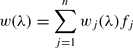
where λ is spectral waveband, n is number of endmembers and fj is relative fraction of component j.
The nonlinear effect in quantifying vegetation spectral reflectance was noticed and sometimes addressed in the spectral mixture analysis (Guan and others Reference Guan, Xie and Zhu2008). Borel and Gerstl showed that nonlinear spectral mixing occurs due to multiple reflection and transmission from surfaces (Borel and Gerstl Reference Borel and Gerstl1994).
Spectral unmixing is a deconvolution technique that aims at estimating the surface fractions of a number of spectral components or endmembers together causing the observed mixed spectral signature of the pixel. A linear combination of spectral endmembers is chosen to decompose the mixed reflectance spectrum of each pixel, R i, into fractions f i of its endmembers j in i bands, Re ji (Meer Reference Meer, Stein, Meer and Gorte1999).
The spectral unmixing model requires a number of spectrally pure endmembers. The tundra-taiga ecotone consists of spectrally very similar vegetation which can be confused even in very high resolution imagery. As different plant species respond differently to energy in the electromagnetic spectrum (Verbyla Reference Verbyla1995), remotely sensed data of high spectral resolution can in theory be used to distinguish between these species. However, Price (Reference Price1994) and Portigal and others (Reference Portigal, Holasek, Mooradian, Owensby, Dicksion, Fene, Elliot, Hall and Driggett1997) demonstrate that the leaf reflectances of different species are highly correlated because of their similar chemical composition, and hence are not unique. Moreover the reflectance spectrum of green vegetation is well known and overall is very similar from species to species (Cipar and others; Sobhan Reference Sobhan2007).
But in spite of this the linear spectral unmixing model is often applied to medium-resolution multispectral data from sensors such as Landsat TM/ETM+ or Terra ASTER for mapping large spatial extents (Mezned and others Reference Mezned, Abdeljaoued and Boussema2010; Yang and Ren Reference Yang and Ren2008; Olthof and Fraser Reference Olthof and Fraser2007). This method does not provide high accuracy of endmember extraction and has certain applicability limits. Due to the shortage of spectral information (only several relatively wide spectral bands present in the imagery) and similarity of endmember reflectances it can lead to the same summary reflectance originating from mixtures of different spectral endmembers with different abundances.
To move towards understanding how accurately we can decompose mixtures in satellite imagery and in order to understand possibilities of spectral unmixing for imagery of the tundra-taiga ecotone we started from the most detailed information at the largest possible scale (ground spectroradiometry data collected in the field). We carried out a field experiment with a portable spectroradiometer to provide many controlled mixtures of typical objects in the tundra-taiga ecotone, to research their spectral properties and to determine what are the implications for unmixing satellite imagery of ecotone areas.
The main goals of this study are: i) to describe the interrelation between mixture spectra and pure spectra composed from specific endmembers present in mixtures; ii) to define threshold values for discernability of endmembers in a spectral mixture on the basis of spectral signatures and mixture colour modelling; iii) to estimate results of linear decomposition of spectral mixtures; iv) on the basis of the obtained results to suggest threshold values and number of classes for vegetation mapping based on the method of spectral unmixing.
Study area
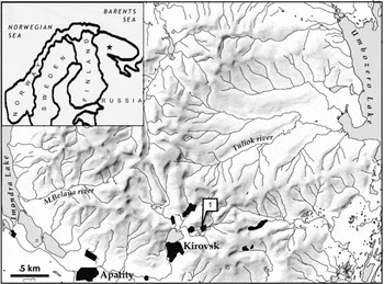
The Khibiny Mountains were chosen for the experiment as being a territory of typical tundra-taiga conditions where the authors have been conducting field research of vegetation for a number of years. The Khibiny Mountains are situated in the centre of the Kola Peninsula in northwestern Russia, 150 km to the north of the Arctic Circle (Fig. 1). The highest peaks lie between 900–1200 m a.s.l. The climatic features and the considerable elevation in comparison with the surrounding plain provide many gradients typical for the tundra-taiga ecotone on the territory of this mountain mass (ca. 2,500 km2). Dense forest dominated by Picea abies, Betula pubescens, with dwarf shrub and moss cover is situated in the bottom parts of valleys and in the foothills. The trees in the forest are usually 5–15 m tall. Mainly at heights from 350 to 450–500 m a.s.l., these forests are replaced with birch krummholz (Betula tortuosa) which sometimes forms a continuous belt but often breaks up into separate spots alternating with mountain tundra vegetation. The mountain tundra belt is typically found from 350–450 m a.s.l. to 600–850 m a.s.l. on slopes and tops of mountains. It consists of patchy tundra, in places dominated by grasses, dwarf shrubs, mosses and lichens depending on microclimate, with significant altitudinal gradient from mostly dwarf shrub tundra (with Betula nana, Empetrum nigrum) to dwarf shrub-lichen tundra, then to lichen-dominated tundra (Cetraria nivalis) and to stony tundra (partial cover of crustose lichens on nepheline syenite rocks which are weathered to different degree). Typical kinds of vegetation for all belts are often similar, but are in different spatially dependent abundance that defines various mixtures.
Region of research. Khibiny research and education station of MSU.

Experiment design
In our experiment we used a Skye Instruments SpectroSense2+ ground spectroradiometer (serial numbers of the sensors 1007 33216, up looking; 1007 33217 down-looking) with the following spectral bands: channel 1 – 449–501nm (central wavelength 475nm, Blue), channel 2 – 497–599nm (546nm, Green), channel 3 – 647–707nm (677nm, Red), channel 4 – 774–900 nm (837 nm, NIR. These spectral bands are similar (though not identical) to the corresponding bands of the popular orbital sensors, such as QuickBird, Landsat TM, Terra ASTER. The SpectroSense2+ instrument has a down looking sensor measuring reflected light within a 25o field of view (FOV) and an up looking sensor fitted with a cosine correcting light acceptance head and simultaneously measuring down welling light within a hemisphere.
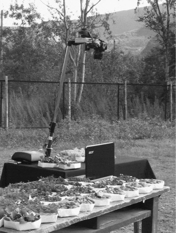
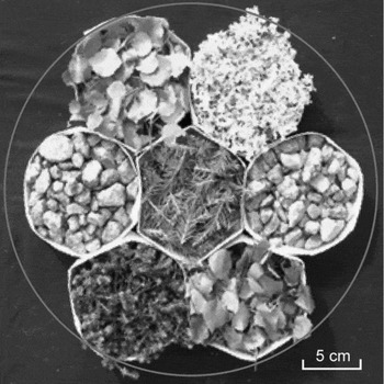
We have collected samples of typical arctic landscape components such as: Cetraria nivalis (white fruticose lichen), birch (Betula tortuosa), dwarf shrubs (Empetrum nigrum, commonly known as crowberry, and Betula nana, or dwarf Arctic birch), Norway spruce (Picea abies) and rocks (nepheline syenite). We have constructed mixed samples with controlled percentages of these components in situ. All samples were harvested and prepared on the same day one hour before the experiment: we have placed them in adjacent paper hexagonal frames 3 cm high (Fig. 2). Samples filled the frames entirely so that paper edges were almost invisible; dwarf shrubs, birch and spruce samples were sliced by scissors. Frames were placed close to each other on the black cloth, filling the circular FOV of the spectroradiometer. We composed hexagonal mixtures within the field-of-view using 7 frames each time, each frame filling almost 12% of the FOV, and black cloth filling 17%. Seven samples of each component type have been prepared, so we were able to construct ‘pure’ samples with all seven frames filled by the same component, and mixtures of different components with the step of about 12% area of the FOV, using various combinations of the frames. Reflectance factors of 299 combinations of frames have been measured. The reflectance of black cloth which participated in all measurements was subtracted in later analyses and areas occupied by the studied components were rescaled to 0–100% range (this was required, in particular, to reduce the number of components to consider in unmixing).
Experiment design: the spectroradiometer is installed above the table covered by black cloth, and samples are moved in specific combinations into the FOV; in addition to the two sensors, a down looking camera is attached to the top of the pole for documentation.

An arrangement of samples as placed in the spectroradiometer's field-of-view (marked with white circle).

The spectroradiometer was established motionlessly, thus, its height was fixed, and the angle between the direction on the sun and on the sample changed only because of the sun movement. The samples were composed to be as flat as possible (height variations of the sample surface generally well below 1 cm) in order to avoid any significant shading inside the sample. The observed shadows were semi-transparent, occupied less than 6.5% of the total area within the FOV and varied by less than 5% of this area.
The experiment took place on 12 August 2010 on a day with partially cloudy sky (providing diffused illumination much of the time) between 14:40 and 18:20 local summer time, in the courtyard of Khibiny teaching and research station of the Moscow State University, Murmansk region, Russia. The station is located near the key sites of the PPS Arctic project of the International Polar Year in which the structure and dynamics of the forest-tundra ecotone has been studied since 2007.
The calibration of the spectroradiometer did not allow making measurements in absolute reflectance units or in reflectance factor at the scale of 0 to 1 due to different geometric setup and calibration of up looking and down looking sensors (B.Trotter, personal communication, November 2010). Raw measurements of all mixtures were recalculated into reflectance factors in nominal (arbitrary) units by simply dividing down looking sensor measurements by up looking sensor measurements. This compensated for temporal variations in solar illumination during the experiment.
Methods
Statistical analysis
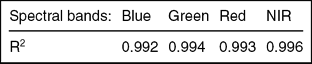
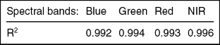
The spectroradiometry data set (299 samples) was analysed statistically. We used multiple linear regression to determine whether a mixture spectrum depended on abundance of several endmembers linearly (see Table 1). Data from each spectral channel were analysed separately; the reflectance factor values were taken as the dependent variable, and percent areas of the six studied components in each sample as independent variables.
Multiple linear regression results between spectra of mixtures and endmember abundances.
Spectral analysis
At first we analysed mixtures of two endmembers then mixtures of three and four endmembers. The combinations most often met in tundra-taiga transition zone were considered (see Table 2). In mixtures 1 to 9 we used two endmembers whose abundance were consistently changed with a step in one hexagonal frame (12 % of the area of the original sample, and just over 14% of the area without the background black cloth). From three- and four- component mixtures we chose those resembling typical heterogeneous landscapes of the tundra-taiga ecotone: transition from dwarf shrub tundra to lichen tundra (No.10) and sparse spruce and birch forest, or transition from forest to dwarf shrubs (No. 11 and 12). Four endmembers are presented in mixture No.10: B. nana, and E. nigrum (this combination is further termed ‘dwarf shrubs’), and lichens and stones (this combination is further termed ‘non-green’). In mixture No. 11 there are three endmembers: B. nana and E. nigrum (collectively dwarf shrubs) and P. abies, while in mixture No.12 there are B. nana and E. nigrum (dwarf shrubs), and B. tortuosa. For three- and four-component mixtures we had to vary the number of frames occupied by different species. For example when there was an even number of frames with dwarf shrubs (B. nana and E. nigrum) that is, to form 28%, 57%, 86% of the mixture, we used equal number of frames for each species. When the number of the frames was odd, we have used one frame more for one of the species, in a random way (it did not influence the result much as these dwarf shrubs have similar reflectance). In the same way we formed mixture No. 10 varying, when necessary, the number of frames with lichens and stones.
Typical mixtures for tundra-taiga ecotone analysed in this research.

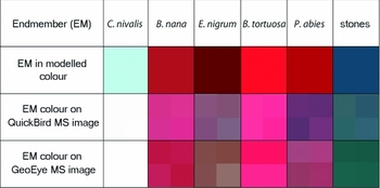
We analysed the separability of mixtures by examining the changes of the mixture reflectance while varying proportions of different endmembers. Since much vegetation mapping is based on analysis of false colour infrared image composites, we have modelled the colour that a particular mixture would have if measured reflectance factors in the near infrared (NIR), red and green band values were plotted as a red-green-blue (RGB) colour composite. To the minimum measured values in each spectroradiometer band we assigned the value of 0, and to the maximum value we assigned 255, while all the intermediate values were stretched linearly. Thus we have modelled the colour that the same object should have in a pixel of a multispectral satellite image (with similar spectral bands) on the computer screen. To check the overall correctness of the approach we have compared the colour of pure ground endmember spectra to the colour of the same endmembers on the extracts of very high resolution multispectral images: QuickBird (spatial resolution is 2.4 m) and GeoEye (spatial resolution 2 m) as shown in Figs. 3a and 3b. The extracts were selected from very small subsets of these images for the Tuliok river valley in Khibiny mountains (where authors have conducted detailed field research). The subsets were stretched linearly. The stretch was done individually for each image to account for radiometric differences, but the identical geographic coverage ensures that the colours are comparable. It was assumed that the temporal differences between the images are small (although the QuickBird image was acquired on 28 June 2006, and the GeoEye image on 20 August 2009), because the endmember extracts were selected far from transition zones which could be influenced by phenology, and the Tuliok area has not experienced any noticeable long term change between 2006 and 2009. Satellite imagery has been converted to reflectance, but atmospheric correction has not been performed. The comparison of image-and ground-measurements derived colour has shown good correspondence of colours and so this approach was adopted.
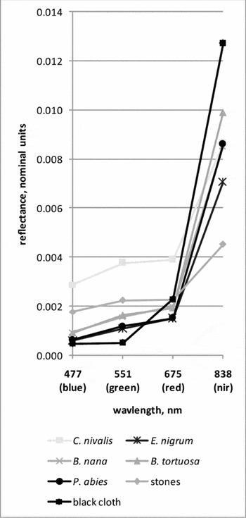
Pure endmember spectra as derived from ground spectroradiometric measurements. Each signature corresponds to seven hexagonal frames filled with the same component. The signature for the background black cloth (measured without frames) is also given for reference (reflectance factor of this cloth has been subtracted from all measurements before processing).

Modelled colour of endmembers (NIR, red, green bands in the RGB 432 model) in comparison with extracts of very high resolution imagery for the same components.

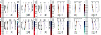
The simulated colours for all mixtures were analysed consistently as components were added and subtracted with a step of 14% abundance (by area) (Fig. 4). The visual threshold of colour change (that is, a change of colour tone appreciable to human eye) was perceived as a signal that the mixture has changed. We intended to find maximum 3 significant colour changes that corresponds to three logical classes of abundance value: ‘endmember (EM) added in small quantity’, ‘EM definitely present’, ‘EM predominates’. Values of abundance for each endmember, causing this change were thus fixed.
Spectral graphs of mixtures depending on component abundance. Under the graphs we show percentages of the components used and simulated colours for false-colour infrared composites.

These thresholds were checked numerically on the basis of the shape of spectral graphs as they changed with addition of various endmembers (Fig. 4). Significant breaks of the green, red and NIR spectral graphs were considered as confirming the visual thresholds; we considered as significant changes of reflectance factor by at least 5% per one 14% step in area abundance of mixture components. The 5% change corresponds to the accuracy of sensor calibration. If changes of the reflectance factors in at least one channel of three (green, red and NIR) were over the 5% of the whole measurements range the visual thresholds were confirmed as significant. Otherwise the visual thresholds were excluded (see Table 3).
End member abundance thresholds (on the basis of mixture colour changes).

Indices: C– C. nivalis, E – E. nigrum, S – stones, BT – B. tortuosa, BN – B. nana, P – P. abies, D – dwarf shrubs, NG – non-green class.
* - thresholds are barely noticeable visually
** - change of reflectance factor is less than 5% of the measurements range
Linear unmixing
Linear spectral unmixing (LSU) was also applied to the set of 299 spectral measurements in order to estimate errors that occur when we try to calculate abundances for typical classes of forest-tundra ecosystems using 4-channel sensor data. This part of the experiment leads to further estimation of the threshold values for abundances in order to classify them further in satellite imagery products. We used some constraints for the unmixing model: 1) abundances are positive or equal to zero; 2) abundances follow in steps of 1/7, 2/7, 7/7 area to form a measurement prediction; 3) the sum of predicted abundances is 100%. Similar to all other analyses, the reflectance factors of the background black cloth was subtracted prior to unmixing from each measurement and then abundances (areas) were rescaled, so that frames with components were assumed to occupy 100% of the measured area. We calculated predicted spectra for all possible mixtures of endmembers using pure endmember spectra and real abundances. Then a spectral distance in 4D space (according to the number of bands) was calculated between each of the predicted spectra and real measured spectra. The equation for the distance calculation is

where B, G, R, NIR are reflectance factor values in blue, green, red and near infrared bands accordingly.
For each predicted spectrum the combination with the least distance was chosen as an estimate of the predicted abundances.
Then we calculated standard deviations (SD) for errors (expected mean for them equals 0) of abundance prediction in unmixing for 6 endmembers and also for 3 group endmembers: trees (B. tortuosa and P. abies), dwarf shrubs (E. nigrum, B. nana) and non-green (C. nivalis and stones). As all classifications of remotely sensed data have errors, but some level of accuracy can be considered acceptable, these deviations allow us to apply an additional assessment to our measurements. For example, if we have 50% of fully correct measurements, but still have the rest of them with high errors the SD value will be high, but if we have 10% of fully correct measurements, and 70% of ‘good’ measurements with errors of 1/7, the SD value will be low. We have then compared SD values with the ranges of abundance derived for each endmember by spectral analysis, in order to define thresholds, describing how many classes of components by abundance we can discern on the basis of linear unmixing.
Results
The obtained spectral data has shown that the spectrum of a mixture is approximately the linear sum of spectra of the constituent endmembers multiplied by their abundances. The determination coefficients (R2) of the regression are high in all channels (see Table 1). We conclude that it is possible to suppose an approximately linear sum of spectral components when scaling up from detailed to less detailed multispectral data.
The results of T-statistic tests show that stones and lichen have the most significant statistical influence on the mixture spectra in most spectral bands, while green plants have significant influence in the NIR and green bands (see Table 2). Thresholds for endmembers defined by mixture colour changes and checked by spectral graphs breaks are presented in Table 3. Some conclusions about endmembers can be made from this analysis:
1. Adding green vegetation into a stone mixture causes considerable changes in the reflectance factor in the visible range when the vegetation occupies 28–43% of the sample area. In the NIR band the values smoothly grow as vegetation is added.
2. Adding C. nivalis into mixtures also causes growing reflectance factors in the NIR band, especially after 57% by area is added. This lichen can be recognised in the mixtures after 14–28% areal abundance.
3. Dwarf shrubs and non-green (lichen and stone) mixtures differ well from each other.
4. Stones predominate by reflectance factor in the stone and lichen mixture if they occupy at least 86% of the area. In mixture with green vegetation, stones have a dominating influence on the reflectance factor if they occupy 71% of the area and in this case they cause a rather sharp colour difference in the false colour infrared composite.
5. The mixtures consisting from green vegetation only cannot be separated well by components. Significant changes occur only in the NIR band and they are rather small to be seen well in the composite colour change and spectral graphs. It is very difficult to find significant thresholds in B. nana and P. abies mixtures. Differences in reflectance factors are less than 5%. On the other hand, dwarf shrubs and B. tortuosa mixtures differ significantly.
We note for spectral graphs of all mixtures that values of reflectance factor in the blue channel are similar and slightly lower than those in the green channel. The blue channel could therefore be considered redundant.
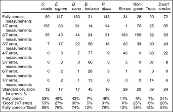
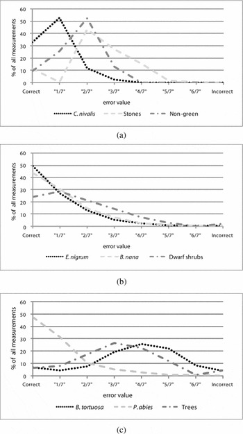
The LSU results are shown in Table 4 and graphically in Fig. 5. When we analysed the accuracy of LSU results we used several definitions: fully correct measurement of endmember; a correct match of predicted and real abundance. A good measurement is when we have a 1/7 error (1 incorrectly identified sample frame out of 7). Overall the LSU analysis shows large errors. B. nana, P. abies and E. nigrum are defined correctly in 40–50% of cases. C. nivalis has a high percentage of ‘good’ definitions by LSU in comparison with the rest of the endmembers.
Linear unmixing results (299 measurements in total).

Evaluation of unmixing results. a. Non-green classes. b. Dwarf shrubs. c. Trees.

Group endmembers were considered as correctly measured only when both of the components were defined correctly. For the ‘non-green’ (lichen and stones) class and dwarf shrubs we have some measurements that were correctly unmixed and the major part of measurements had errors of less than 3/7 (Fig. 5). For most of the measurements (except B. tortuosa) the unmixing errors are within error limits of 2/7 to 3/7, so the threshold value for abundance classification is between 29–42% that basically corresponds to two or three classes of components by abundance discernible in the dataset. But a many results have inaccurate abundances, especially for B. tortuosa and stones. The reason of this could be that we have only 4 channels of data for 6 classes, but actually mixtures of 4 or fewer classes were also unmixed incorrectly. B. tortuosa was confused with E. nigrum, P. abies and with B. nana in combination with the ‘non-green’ class. Therefore trees were unmixed not so well, mainly because of incorrect estimation of B. tortuosa.
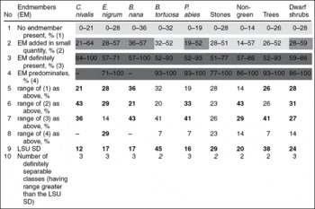
In Table 5 we compare the endmember abundances thresholds from Table 3 (received from colour change and spectral graphs analyses) with standard deviations for errors for the same endmembers received from unmixing. In rows 1–4 there are 4 classes for each endmember that were defined from mixture colour change and spectral graph analyses. The boundaries of classes for each endmember are mean threshold % area values from all mixtures containing this endmember (see Table 3). The ranges of these classes are calculated in rows 5–8. In row 9 we display the standard deviation value (SD) for each endmember from the LSU results. Comparing ranges of classes and the SD we can conclude which classes could be defined correctly through linear unmixing (their range should exceed the SD). Almost all mixtures could be definitely separated into 2 or 3 classes with some indication of abundance. For example abundance of B. tortuosa and also abundance of all trees (because of the B. tortuosa) can be defined in only 2 classes: ‘few birches/trees’ and ‘many birch/trees’. If the range for a class is less than SD from the LSU analysis, we aggregated this class to the next by abundance. If SD is higher than every range of classes defined in the threshold analysis, we assume that a maximum of 2 classes may be separated, that is, presence of a component without indication of abundance, and its absence. Discernible classes in Table 5 are marked with shading in the cells. If classes are aggregated, they are shown with the same shading.
Mean abundance ranges for discernible endmembers (EM), in comparison with standard deviation of abundance derived through linear spectral unmixing LSU SD (as given in Table 4). Ranges that exceed the LSU SD are in bold. When all ranges are less than SD, the discernible number of classes is shown in italics (only absence/presence of a class can be indicated). Aggregation of abundance classes derived from this comparison is shown by grey shading of the class cells (in each column, the same shading corresponds to one class).

Discussion
We make several further observations from the results of this study:
1. The multiple regression analysis shows that spectral mixtures of components typical for the forest-tundra ecotone can be analysed qualitatively using the linear mixing model. Quantitative analysis could be difficult due to insufficiently high R2. This subsequently shows up in the large errors of linear decomposition of our set of 299 samples.
2. Lichens are shown as having most influence on the spectral mixtures, which is also the phenomenon we noted in interpreting Terra ASTER and Landsat TM and ETM+ imagery of the tundra-taiga ecotone areas. They are subsequently showing the best results in linear unmixing. The high errors of linear spectral unmixing experiment are most possibly caused by the small number of spectral channels and high correlation between them especially in visible range as indicated in Fig. 4. Similar spectral signatures of the endmembers also negatively affect the results. Additional difficulties are caused by presence of 6 components (although in combinations of not more than 4) in the data, while only 4 spectral channels are available in the data.
3. In our experiment, we did not considered the influence of drying on reflectance of the samples. This could be significant for B. tortuosa leaf samples which are most prone to drying out of the six surface types we examined. However, the whole experiment lasted only for three hours. Besides, the most prominent effects of drying on reflectance would be observed in the water absorption bands in the near infrared part of the spectrum (Ollinger 2010), which is outside our measurement range. For lichen samples dried over 2–3 days, Rees and others (Reference Rees, Brown, Mikkola, Virtanen and Werkman2004) indicated 5–10% change in reflectance. We suppose that possible change of reflectance over the duration of the experiment was small in comparison to influence of particular components on reflectance.
4. The abundance thresholds of the studied components, allowing the separation of up to 3 classes can be used for interpretation of high and medium resolution multispectral satellite imagery and to guide spectral unmixing of such imagery. However, this will require atmospheric correction of the imagery and consideration of scaling effects. For example Zeng and others (Reference Zeng, Schaepman, Wu, Clevers and Bregt2007) note only partial correspondence (R2 = 0.60) between forest crown closures derived by linear spectral unmixing from EO-1 Hyperion images using QuickBird images to estimate endmember abundances, and ground data.
5. Obviously additional channels will help linear spectral unmixing. As many studies show, the most informative spectral region is the SWIR which indicates the strong potential for using this spectral region in mixture decomposition (for example Asner and Lobell Reference Asner and Lobell2000). Such channels are present in Landsat ETM+, SPOT HRVIR, and Terra ASTER imagery and thus are widely applicable. We intend to continue this experiment in summer 2011 (when we hope to obtain a ground hyperspectroradiometer), and to develop this work further and work on the upscaling of these results to analysis of satellite imagery of various resolutions.
6. Further investigation will be also focused on testing statistical approaches that may possibly perform better than a physical unmixing approach when few channels are available and the problem is underdetermined.
7. We should note that when unmixing satellite imagery, the results will be further complicated by natural variability of endmember reflectance for various vegetation species and rock types met in the real forest-tundra ecotone.
Conclusions
1. The linear model of mixing is applicable to mixtures in the experiment, with R2 over 0.99. This considerably simplifies consideration of influence of components and allows the use of linear unmixing.
2. Stones and lichens can be recognised in the mixtures when they occupy 86% and 57% respectively, green vegetation of the experiment is recognisable after 43% abundance. These are the most accurate area thresholds that can be defined with the available ground spectroradiometry data and we assume that they are more accurate than thresholds discernible from satellite multispectral imagery such as ASTER, TM, ETM+. Almost all green vegetation hardly differs in 4 spectral bands except mixtures with B. tortuosa, but it differs much better from the non-green (stones + lichen) group.
3. The real definition of most components (except B. tortuosa) in the linear unmixing experiment based on ground data is not very successful. In most cases it is within error limits of 3/7 and C. nivalis has the highest percentage of good definitions by LSU in comparison with the other endmembers. P. abies, E. nigrum and B. nana also have applicable result if we consider ‘good’ measurements as applicable.
4. In comparing ranges of abundance discernible for component classes, defined from analysis of measured spectroradiometry data, and standard deviations of linear unmixing carried out for the same data, we conclude that most components in the mixtures could be separated into 2 or 3 classes by abundance (including the absence class).
Acknowledgements
We thank Belinda Trotter of Skye Instruments Ltd. for help with spectral data calibration and an anonymous reviewer for useful comments on this manuscript. This research is part of PPS Arctic, the IPY project which investigates current status and past changes in the circum-arctic tree-line zone, as well as associated social and natural factors. The study is carried out in the Laboratory of Aerospace Methods of the Faculty of Geography, Lomonosov Moscow State University, Moscow. The authors are financially supported by the Benefits Russo-Norwegian project of the Norwegian Research Council to Dr Annika Hofgaard (OST 185023/S50), by the Leading Science Schools programme of Russian Federation, grant no. 3405.2010.5171 and Russian Scientific Educational Centres programme grant no. 14.740.11.0200.