1. INTRODUCTION
Unmanned surface vehicles (USVs) have great potential for application in both military and civilian fields. The technology of automatic collision avoidance is one of the key technologies needed to realise the automatic navigation of USVs (Statheros et al., Reference Statheros, Howells and Maier2008; Park and Yoo, Reference Park and Yoo2019). Much progress has been made in research into collision avoidance under static and known environments, while dynamic collision avoidance under unknown environments is becoming a hot topic in the field of USVs (Fan and Li, Reference Fan and Li2017; Chu and Zhu, Reference Chu and Zhu2018). Cheng et al. (Reference Cheng, Sun, Huang and Zhang2019) introduced fuzzy logic into the USV control system, and a deep reinforcement learning framework based on expert experience was established. Wang et al. (Reference Wang, Zhang, Sun, Cao, Wan, Sheng and Liu2019) proposed an optimal weight distribution algorithm for collision avoidance by the dynamic path planning method. Tam et al. (Reference Tam, Bucknall and Greig2009) and Fişkin et al. (Reference Fişkin, Kişi and Nasibov2018) also adopted this method. The problem of avoiding collision by path-following control has been widely studied (Xargay et al., Reference Xargay, Kaminer, Pascoal, Hovakimyan, Dobrokhodov, Cichella and Ghabcheloo2013; Lu et al., Reference Lu, Zhang, Sun and Zhang2018; Zhang et al., Reference Zhang, Deng, Zhang and Huang2018a, Reference Zhang, Huang, Zhang and Zhang2018b; Qin et al., Reference Qin, Wu, Sun and Sun2019; Xu et al., Reference Xu, Rong and Soares2019). The neural network method has been successfully used in dynamic collision avoidance with low real-time requirements (Liu et al., Reference Liu, Wang, Peng, Chen and Li2019; Huang et al., Reference Huang, Chen, Chen, Negenborn and van Gelder2020). The velocity obstacle method ingeniously transforms the collision avoidance problem in position space into the velocity space (Fiorini and Shiller, Reference Fiorini and Shiller1998).
When navigating in complex and changeable dynamic environments, USVs are not always equipped to meet the complex control laws produced by analytic algorithms (Cheng et al., Reference Cheng, Sun, Huang and Zhang2019). Therefore, practical and simple collision avoidance algorithms in complex environments still need to be studied.
The artificial potential field (APF) method has the advantages of being simple, safe and reliable (Khatib, Reference Khatib1986). It can quickly plan a global path for the known environment with only static obstacles. For the unknown environment with dynamic obstacles, however, it is difficult for the algorithm to play a role. By using the resultant force as the driving force of the USV, dynamic navigation control based on the APF method can be realised. The APF method has sensitive hazard perception ability; as the distance between the USV and an obstacle decreases, the repulsive field tends to grow exponentially and far exceeds the ultimate dynamic performance of the USV. At the same time, the APF method only judges the risk of obstacles by distance, that is, as long as the USV passes through the vicinity of the obstacle, it will make meaningless detours, which increases the length of the path. Therefore few scholars apply the APF method to the dynamic collision avoidance of USVs. Yao et al. (Reference Yao, Zhou, Zhang and Dong2010) improved the traditional APF method by introducing a repulsive constant fuzzy controller for the UAV to avoid dynamic obstacles. Song et al. (Reference Song, Su, Dong, Shen, Xiang and Mao2018) improved the repulsive field on the basis of traditional APF, which was composed of repulsive potential field and centrifugal potential field. The improved APF algorithm was applied to dynamic obstacle avoidance by USVs.
The APF method can solve the path planning problem well in a static environment. For the real-time collision avoidance problem of dynamic obstacles, however, APF usually only considers the relative distance between the USV and the obstacle and ignores the effect of relative speed on the collision risk. The APF method has good risk sensitivity and can be used to evaluate the risk. The collision cone has the ability of risk identification. These two characteristics can be combined well. In this algorithm, collision risk is related not only to the relative distance, but also to the relative speed. The main features of the proposed LAPF-CC algorithm are summarised as follows:
1. A new improved APF method is proposed to improve the attractive force. The relative effects of attractive force and repulsive force are not affected by the distance between USV and target, and the unexpected component of the repulsive force is avoided.
2. The driving force and torque of the USV are controlled separately. By applying this strategy, the APF method can be applied to the dynamic collision avoidance control of the underactuated USV. The deviation between the current heading and the ideal heading is used as the input of control.
3. In order to prevent the relative velocity from causing the USV to enter and leave the collision cone frequently, the velocity locking state is designed, which improves the stability of control and the safety of collision avoidance over a short distance.
4. According to the risk factors of collision, the innovation of speed torque is introduced to realise the smooth control of torque.
5. Based on the APF algorithm, the potential field is layered, which can identify the risk level more accurately, choose the appropriate collision avoidance strategy better, and avoid unnecessary collision avoidance actions.
This paper is organised as follows. Section 2 presents the motion model, Section 3 presents the LAPF-CC algorithm. In Section 4, the strategy of the LAPF-CC algorithm is designed, and the simulation results are presented in Section 5. This paper is completed with some concluding remarks in Section 6.
2. MOTION MODEL OF THE USV
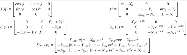
This paper mainly studies the movement in the horizontal plane (Fossen, Reference Fossen2011; Zhang et al., Reference Zhang, Deng, Zhang and Huang2018a, Reference Zhang, Huang, Zhang and Zhang2018b). The main motion variables are the surge velocity u, the sway velocity υ, and the yaw velocity r in the body-fitted frame, as shown in Figure 1. The ship motion equation is simplified as follows.
 $$\begin{align} \dot{\eta} &= J( \eta) \nu\\ M\dot{\nu} + N( \nu ) \nu &= \tau + {\tau_w} \end{align}$$
with the position vector  $\eta \stackrel{\rm def}{=}\, [ x\ y\ \psi] ^{T}$, and the velocity vector
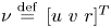 $\nu \stackrel{\rm def}{=}\, [ u\ v\ r] ^{T}$. (x y) is the trajectory coordinates and ψ is the heading angle. J(η) is the transformation matrix, all parameters are shown in Table 1.
 ${\rm M}\dot{\nu}$ is used to describe the inertia force, M is the inertia matrix (Perez, Reference Perez2006), m is the mass of the USV, I z is the rotary inertia of the z-axis for the USV.
 $X_{\dot{u}}$,
 $Y_{\dot{\nu}}, \; Y_{\dot{r}}, \; N_{\dot{\nu}}, \; N_{\dot{r}}$ are coefficients of additional mass.
 ${\rm N}( \nu ) \nu$ is used to describe hydrodynamic and hydrostatic forces. The effects of Coriolis centripetal force and fluid damping force are considered,
 $N( \nu) \nu =C( \nu) \nu +D( \nu) $. The damping force includes two parts (Zhang et al., Reference Zhang, Huang, Zhang and Tian2019): linear damping and nonlinear damping, i.e.,
 $D( \nu) =D_{L} ( \nu) \nu +D_{NL} ( \nu) $; among them
 $X_{u}, \; Y_{v}, \; Y_{r}, \; \ldots, \; N_{vvr}, \; N_{rrr}$ are the hydrodynamic coefficient.
 $\kappa \in \mathbb{R}^+$.
 $\tau =[ \tau_{u} \quad \tau_{\nu} \quad {\tau_{r}}] ^{T}\in \mathbb{R}^{3}$, which represents the control force or torque provided by the servo system. τu represents the thrust generated by the propeller to drive the USV forwards and backwards. τr represents the moment that drives the USV to turn. For the underactuated USV, τν = 0. τw represents the disturbing forces or moments generated by the ocean, including the impacts of wind, waves and currents,
 $\tau_{w} =\tau _{{\rm wind}} +\tau_{{\rm wave}} +\tau_{{\rm current}} \in \mathbb{R}^{3}$. In order to simplify the problem, the influence of τw is ignored;
 $\tau_{w} \, \stackrel{\rm def}{=}\, 0$.
Description of variables for ship motion.

Parameters of the model.

3. ALGORITHM DESCRIPTIONS
3.1. Layering of dangerous situations
Both the USV and the obstacle are simplified as circles, and their radii are respectively R USV,  $R_{\textit{ObstB}_{i}}$. The USV is considered as a particle, whose radius is expanded to the size of the obstacle ship Bi,
 $R_{B_{i}} =R_{\textit{USV}}+R_{\textit{ObstB}_{i}} + d$.
 $R_{B_{i}}$ is the radius of obstacle Bi after expansion, d is the safety distance.
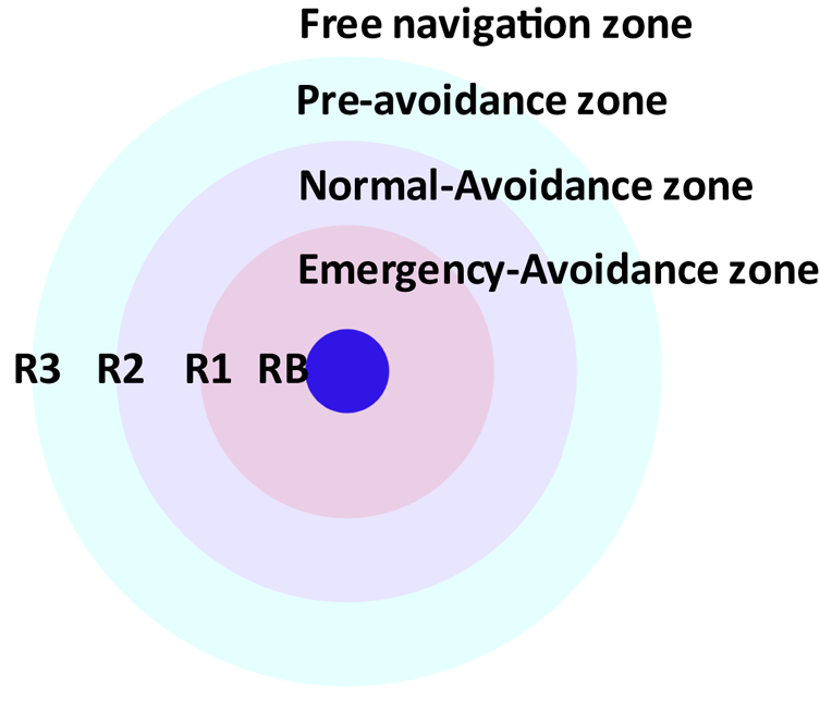
The impact range of the repulsive potential field is divided into four layers from the outside to the inside, whose boundaries are circles with radii of R 3i, R 2i, R 1i, R Bi, as shown in Figure 2.
Layering for the artificial potential field (APF).

In the free navigation layer (d AB > R 3i), since the USV is far enough from the obstacle, the impact of the obstacle does not need to be considered, and the USV only needs to consider the task of navigating to the target. In the pre-avoidance layer  $(R_{2i} \lt d_{AB} \le R_{3i}) $, the USV has entered the impact range of the obstacle, however, it is still far away from the obstacle. There is a possibility that the obstacle ship will suddenly change course, so it is unnecessary to take excessive actions for collision avoidance. Two tasks (collision avoidance and navigating to the target) should be considered comprehensively. In the normal avoidance layer
 $(R_{1i} \lt d_{AB} \le R_{2i})$. Although it is still possible to consider both tasks, the USV should take enhanced collision control actions as it moves into a more dangerous area. In the emergency avoidance layer
 $(R_{Bi} \le d_{AB} \le R_{1i})$, which is a high-risk situation, the USV should ignore the task of navigating to the target and turn quickly to avoid the obstacle.
3.2. APF with collision cone
In the classical APF method, as long as the USV enters the range of the potential field of the obstacle, it will be affected and start to avoid the obstacle, which is sometimes unnecessary. This kind of influence may even cause the algorithm to fall into local optimisation. This paper introduces a collision cone, which can be used to determine whether there is a collision threat. The positions of the USV and the obstacle boat B i are respectively P A (t), P Bi(t) at time t, the velocities are respectively  $v_{A} ( {\rm t}), \; v_{Bi} ( {\rm t}) $, and their angles to the x axis are respectively
 $\alpha, \; \beta$. The relative velocity is
 $v_{BiA} =v_{A} -v_{Bi}$. The angle between v BiA and the x axis is θBiA, and the angle between v BiA and AB is θ, as shown in Figure 3.
Collision cone.

The angles between tangent  ${\rm T}_{L}, \; {\rm T}_{R}$ and x axis are respectively
 ${\lambda}_{1}, \; {\lambda}_{2}$. Based on the x axis, it is positive in the counterclockwise direction and negative in the clockwise direction. This can be seen from the calculation
 $$\theta =\theta_{BiA} -\frac{\lambda_1 -\lambda_2}{2}-\lambda_2$$
The cone area enclosed by two tangent lines TL, TR and circle B is the collision cone. If the ray λBiA from point A along the v BiA direction falls into the cone area  $( v_{BiA} \in {\rm CC}) $, that is to say, when
 ${\lambda}_{2} \le \theta_{BiA} \le {\lambda}_{1}$, it can be considered that the USV will collide with the obstacle at some time in the future. As shown in Figure 3, the area obtained by translating the collision cone by v A is called the absolute collision cone (ACC). Since the end point of v A in ACC is equivalent to
 $v_{BiA} \in {\rm CC}$, in the environment of multiple obstacles, ACC plays a very important role. If the end point of v A is adjusted beyond
 ${\rm ACC}_{1}, \; {\rm ACC}_{2}\ldots$, the USV can avoid all obstacles. By introducing the collision cone into the APF, the following situations are obtained.
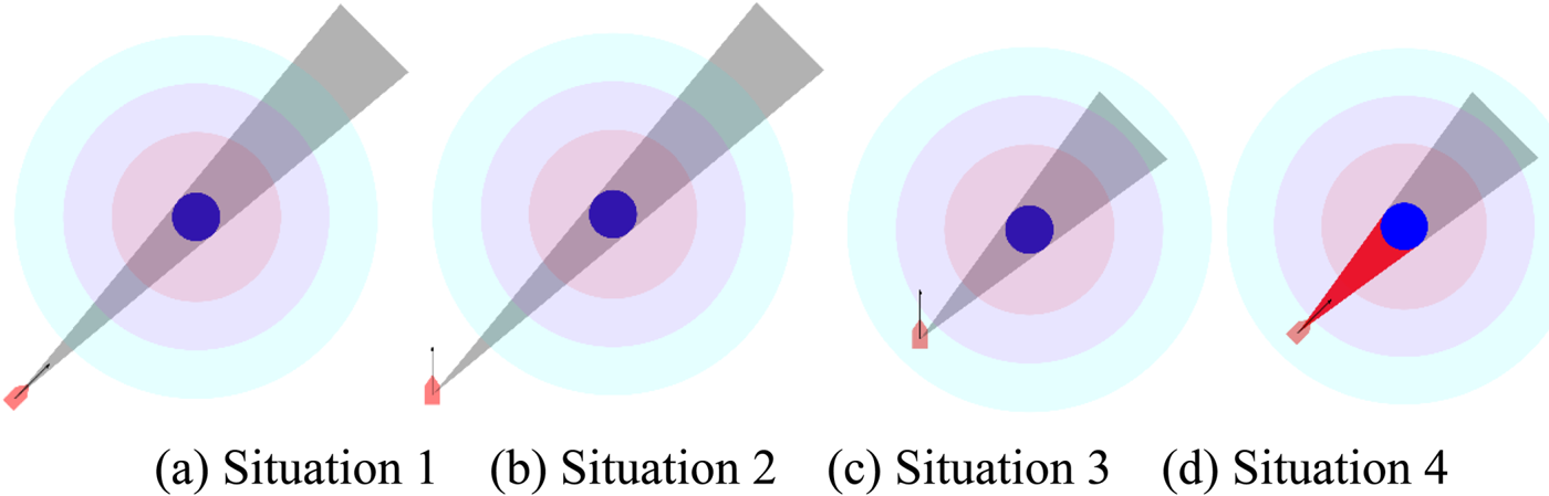
In Figure 4(a) and (b), the USV is beyond the range of the repulsive potential field, that is to say, Equation (3) is satisfied
Artificial potential field with the collision cone: (a) Situation 1, (b) Situation 2, (c) Situation 3, (d) Situation 4.

 $$\mathcal{L}_1 :{\rrho}( {P_A, P_{Bi}} ) >R_3$$
The repulsive potential field will not affect the USV.
In Figure 4(c), the USV is within the range of the repulsive potential field, but v BA is outside the collision cone, which satisfies Equation (4)
 $$\mathcal{L}_2 : \left\{\left[{\rrho}({P_A, P_{Bi}})\le R_3 \right]\wedge \left[\lambda ( {A,v_{BiA}} )\cap \odot Bi=\emptyset \right]\right\}$$
The USV only navigates under the effect of the attractive potential field.
In Figure 4(d), when the USV is in the range of the repulsive potential field and v BA is in the collision cone, Equation (5) is satisfied
 $$\mathcal{L}_3 :\left\{\left[{\rrho}({P_A, P_{Bi}})\le R_3 \right]\wedge \left[\lambda ( {A,v_{BiA}} )\cap \odot Bi\ne \emptyset \right]\right\}$$
There is a risk of collision, so the repulsive force comes into play.
3.3. Potential function model of the LAPF-CC
In the traditional APF method, the effect of the attractive force of the target on the USV will decrease as they approach each other, but the repulsive force is not affected by this, which will lead to the imbalance of the relative influence of repulsive force and attractive force. This is why many scholars multiply the repulsive potential field by the distance between the USV and the target in their work to improve the APF. But after doing that, a component of the repulsive force will appear after derivation, which is not a desired outcome. In this paper, an innovative way of dividing attractive force by distance is proposed, so that the relative effect of attractive force and repulsive force will not be affected by the distance between USV and the target, and the generation of an unexpected repulsive component is avoided. The improved attractive force is
 $$F_{att} ({P_A})=-\frac{\nabla U_{att} ({P_A})}{{\rrho}( {P_A, P_G}) }=\xi \mathop{\to}\limits_{n_{AG}}$$
In the LAPF-CC algorithm, the attractive force of the target to the USV is as follows
 $$F_{att} ({P_A})=\begin{cases} 0, & [ {R_{Bi} \le {\rrho}( {P_A, P_{Bi}} ) \le R_{1i}} ] \wedge [ {\lambda ( {A,v_{BiA}}) \cap \odot Bi\ne \emptyset} ] \\ \xi \mathop{\to}\limits_{n_{AG}}, & {{\rm others}}\\ \end{cases}$$
The repulsive force of the obstacle B i to the USV is as follows
 $$\begin{align}\label{eq8} & F_{repi} ({P_A})\nonumber\\ &\enspace =\begin{cases} 0, & {{\rm others}} \\ \mu \left(\frac{1}{\rho_{( {P_A, P_{Bi}}) }}-\frac{1}{R_{3i}}\right)\frac{1}{\rho^2( {P_A, P_{Bi}}) }\mathop{\to}\limits_{n_{BiA}}, & [ {R_{Bi} \le {\rho}( {P_A, P_{Bi}}) \le R_{3i}} ] \wedge [ {\lambda( {A,v_{BiA}}) \cap \odot Bi\ne \emptyset}] \\ \end{cases} \end{align}$$
The intensities of the potential fields are adjusted accordingly in Equations (7) and (8), so the USV can take specific avoidance actions.
3.4. The model of risk factors for collision
θBiA is the basis for judging whether there is a collision risk. However, it is necessary not only to judge whether there is a risk but also to study the risk quantitatively. As can be seen in Figure 3, the collision depends on two variables: v BiA and  $\rho( {P_{A}, \; P_{Bi}}) $. We define two relevant elements of the model: risk factor of relative velocity and risk factor of relative distance.
When the value of v BiA is fixed, the smaller the value of θ, the greater the collision risk. When the value θ is fixed, the greater the value of v BiA, the greater the collision risk, so we call the projection of v BAi on AB ‘the risk of relative velocity’. The normalised risk factor of relative velocity is  $R_{v_{BiA}}$
 $$R_{v_{BiA}} =\frac{v_{BiA}}{v_{BiAmax}}cos\left( {\theta_{BiA} -\frac{\lambda_1 +\lambda_2}{2}} \right)$$
where v BiAmax is the maximum relative velocity,  $v_{BiAmax} =\vert {v_{A}}\vert +\vert {v_{Bi}}\vert $.
When  $\rho ( P_{A}, \; P_{Bi}) \ge R_{3i}$, there is no collision risk, while as the distance decreases the risk of collision increases. So
 $\rho ( {P_{A}, \; P_{Bi}}) $ can be used to indicate the current risk, which is called ‘the risk of relative distance’. After normalisation, the risk factor of relative distance can be obtained that,
 $$R_{\rho({P_A, P_{Bi}})} =\begin{cases} \left({\frac{1}{\rho ( {P_A, P_{Bi}} ) }-\frac{1}{R_{3i}}}\right)\rho ( {P_A, P_{Bi}}), & {\rho ( {P_A,P_{Bi}} ) \le R_{3i}} \\ 0, & {\rho ( {P_A, P_{Bi}} ) >R_{3i}} \\ \end{cases}$$
Based on the above discussion, the risk factor of obstacle Bi on the USV is R BiA,
 $$R_{BiA} = R_{v_{BiA}} R_{\rho ({P_A,P_{Bi}})} = \begin{cases} \left(\frac{1}{\rho( {P_A, P_{Bi}}) }-\frac{1}{R_{3i}}\right)\rho ( {P_A, P_{Bi}}) \frac{v_{BiA}}{v_{BiAmax}} {\rm cos}\,\theta, & {\rho ( {P_A, P_{Bi}} ) \le R_{3i}}\\ 0, & {\rho ( P_A, P_{Bi} ) >R_{3i}}\\ \end{cases}$$
The torque produced by relative velocity is called ‘speed torque’. Under the effect of R BiA, speed torque drives the USV to turn, where,
 $$M_{BiAr} =M_{max} R_{BiA}$$
M max is the maximum torque of the USV. The direction can be determined by the relationship between θBiA and λ1, λ2. If  $( \lambda_{1} +\lambda_{2} ) /2\lt\theta_{BiA} \lt\lambda_{1}$ then speed torque drives the USV to TL side. If
 $\lambda_{2} \lt\theta_{BiA} \lt( \lambda_{1} +\lambda_{2} ) /2$ then speed torque drives the USV to TR side.
3.5. Action scope of LAPF-CC
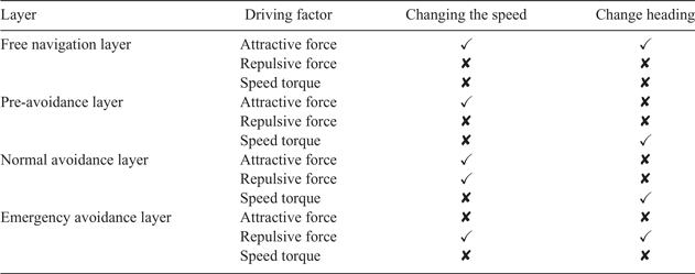
We stipulate that attractive force and repulsive force can change the speed and heading angle of the USV, and speed torque can only change the heading angle. The action scope of LAPF-CC is defined, as shown in Table 2. In the free navigation layer, only attractive force works, which affects both the speed and heading. When the bow direction is exactly the same as the attractive force, the USV navigates towards the target with maximum horsepower. Otherwise, the USV will turn under the attractive force. In the pre-avoidance layer, attractive force changes the speed and speed torque changes the heading angle. In the normal avoidance layer, the USV should adjust v BA out of the collision cone (move the end point of v A out of the ACC) as soon as possible, it should change the speed under the impact of attractive force and repulsive force, and change the heading angle under the action of speed torque. In the emergency avoidance layer, repulsive force is responsible for adjusting the speed and heading angle.
The action scope.

When the USV is at point A, the resultant force is
 $$F_{{\rm total}} ( P_A) =\chi F_{att} ( {P_A} ) +\sum\limits_{i=1}^n {{\rm {\rm K}}_i F_{repi} ( {P_A} ) }$$
χ and Ki are the decision coefficients of the layer, if the USV is in the emergency avoidance layer, χ = 0, otherwise χ = 1. If the USV is located in the range of the repulsive force generated by obstacle B i, then Ki = 1, otherwise Ki = 0.
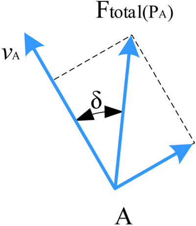
The speed and heading angle should be controlled separately, the speed should be adjusted by driving force, and the heading angle should be adjusted by torque. As shown in Figure 5, δ is the angle between v A and resultant force  $F_{{\rm total}} ( P_{A}) $, and
 $\delta \le \pi$. The factor of driving force is defined as λd, and the factor of torque is λt, then
Analysis of force and velocity.

 $$\begin{align} {\lambda}_d &=\cos {\delta}\label{eq14} \end{align}$$
 $$\begin{align} {\lambda}_t &=\frac{{\delta}}{\pi}\label{eq15} \end{align}$$
In this paper, the maximum driving force of the USV is F max, and the maximum torque is M max. The driving force in the direction of resultant force in the potential field could be defined as,
 $$F_{{\rm LAPF}-{\rm CC}} =F_{{\rm max}} {\lambda}_d =F_{{\rm max}}\cos {\delta}$$
The torque of the potential field could be defined as,
 $$M_{{\rm LAPF}-{\rm CC}} =M_{{\rm max}} {\lambda}_t =M_{{\rm max}}\frac{{\delta}}{\pi}$$
4. LAPF-CC STRATEGY
4.1. Definition of navigation state
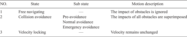
According to the state of the USV and the obstacle, we define three states, as shown in Table 3.
Navigation state of the USV.

Note:‘—’ means there is no sub state.
Free navigating state means that the only task for the USV is to navigate to the target. In the collision avoidance state, when multiple obstacles pose threats to the USV, the impacts of these threats should be considered simultaneously. When the collision risk is cancelled, in order to prevent the USV from entering the collision avoidance state again, the USV is in the velocity locking state, the speed and heading are constant.
4.2. Locking factor
When the relative velocity v BiA of the USV and the obstacle moves out of the collision cone, under the impact of attractive potential field, v BiA is likely to re-enter the collision cone and create a new collision risk. In order to prevent v BiA from entering and leaving the collision cone frequently, when v BiA moves out of the collision cone, while it has the risk of re-entering the collision cone, the navigation state of the USV is set as the velocity locking state, which improves the control stability and the safety of collision avoidance over a short distance. Whether the USV is in the velocity locking state is determined by the locking factor. As long as there is a locking factor, the USV is in the velocity locking state. When all the locking factor disappears, the USV exits the velocity locking state. The generation and cancellation conditions are as follows.
4.2.1. Generation of locking factor
If obstacle i was a threat at the last moment, that is  $[ R_{B} \le d_{ABi} \le R_{3i}] \wedge [ \lambda ( {A, \; v_{BiA}}) \cap \odot Bi\ne \emptyset] $. After taking actions for collision avoidance, they meet
 $[ R_{B} \le d_{ABi} \le R_{1i}] \wedge [ \lambda ( {A, \; v_{BiA}}) \cap \odot Bi=\emptyset] $. In order to prevent the USV from entering the dangerous area again under the impact of attractive potential field, the speed of the USV needs to be locked. We define the obstacle i as the locking factor Υ i.
4.2.2. Cancellation of locking factor
The locking factor will be cancelled if any of the following cases occurs:
(a) when the distance between them is greater than R 3i,
(b) when the USV in the locking state is threatened by an obstacle j, condition
 $[R_{B} \le d_{ABj} \le R_{3j}] \wedge [\lambda ({A, \; v_{BjA}}) \cap \odot B_{j} \ne \emptyset ]$ is met, the locking factor should be cancelled,
(c) when the USV starts to move away from obstacle i.

4.2.3. Switch strategy of navigation state
To simplify the description of switching strategies, we first define the switch conditions, as shown in Table 4:
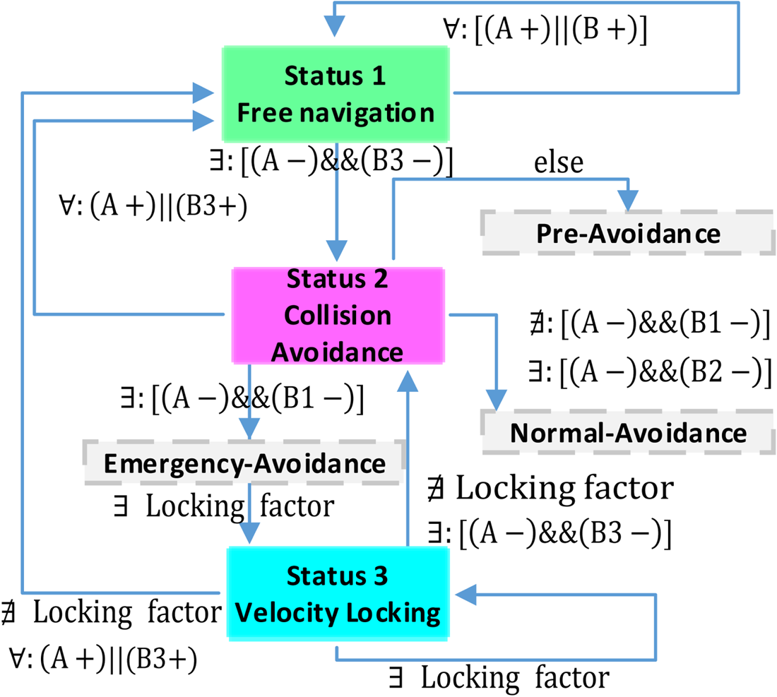
1. When the following condition is met, the USV needs to be switched to free navigating state. The condition
$( A+) \parallel ( {\rm B}3+) $ is satisfied for any obstacle when there is no locking factor.2. When one of the following conditions is met, the USV switches to collision avoidance state.
(a) The USV was in free navigating state or collision avoidance state at the last moment, while there is an obstacle at the current moment, which satisfies the condition
$( {A-}) \& \& ( {B3-} ) $.(b) The USV was in velocity locking state at the last moment, but there is no locking factor at the current time, while there is an obstacle at the current moment, which satisfies the condition
$( A-) {\&}{\&}( B3-) $. In the collision avoidance state, if there is an obstacle that meets the condition $( {A-}) \& \& ( {B1-}) $, the USV switches to the emergency avoidance state. If there is no obstacle that satisfies condition $( {A-}) \& \& ( {B1-}) $, but there is at least one obstacle that satisfies condition $( {A-} ) \& \& ( {B2-} ) $, the USV switches to the normal avoidance state. In other cases, the USV switches to the pre-collision avoidance state.(c) When the following condition is met, the USV needs to be switched to velocity locking state. The USV was in collision avoidance state or velocity locking state at the last moment, while there is a locking factor at the current moment.


The switching diagram of the state is set out in Figure 6.
Switching diagram of the navigation state of the USV.

Switch condition.

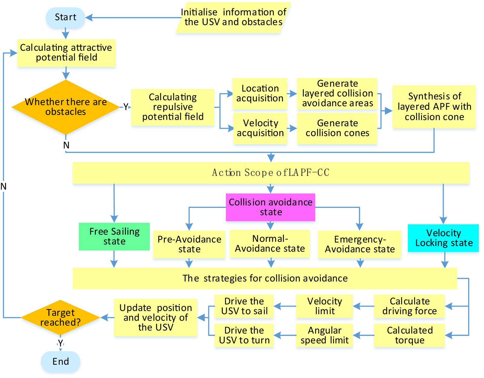
4.3. The process of the strategy for collision avoidance
The process of the strategy for collision avoidance is shown in Figure 7.
Flow chart of collision avoidance.

Assume that the USV detects N obstacles by radar  ${\rm Obst} (N) = [{B_{1}, B_{2}, \cdots, B_{N}}]$. The information of obstacle B i includes the position
 $P_{B_{i}}$, the radius
 $R_{\textit{ObstB}_{i}}$, the speed
 $v_{B_{i}}$ and the heading angle of obstacles
 $\beta_{B_{i}}$.
 ${\rm Info}(B_{i}) = [{P_{B_{i}}, \; R_{ObstB_{i}}, \; v_{B_{i}}, \; \beta_{B_{i}}}]$. The pseudo code of LAPF-CC is shown in the following ‘LAPF-CC algorithm’
5 SIMULATION RESULTS AND ANALYSIS
The study was programmed by C{#} script which linked the MATLAB calculation with the 3D development software Unity by dynamic link library. The computer configuration is as follows: Intel Core i7-9750H six core processor, NVIDIA GTX1660Ti 6 GB graphics card, 16 GB DDR3L memory. The dynamic performance data is measured by the USV platform of IPAC (Information Processing and Advanced Control Group) of Shanghai Jiaotong University. The dynamic performance of the USV is within its limit power range, and its motion ability is controllable.
5.1 Collision avoidance case for single obstacle
5.1.1 Two ships meet on parallel course at low speed
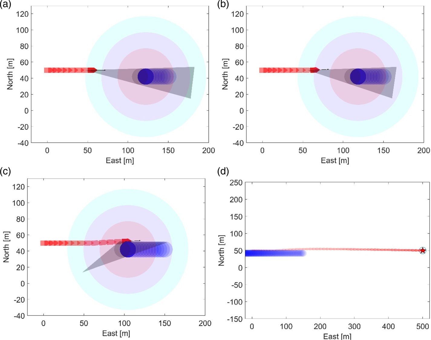
In Figure 8, the obstacle boat is the blue circle, the USV is the red boat. The grey triangle shadow area is the ACC at the current time. The unit of length is m, and the unit of velocity is m/s. The initial position of the USV is (0, 50) and the initial speed is (5, 0). The initial position of the obstacle boat is (150, 42) and the initial speed is (−3·5, 0).
The whole process of collision avoidance at low speed: (a) step 9, (b) step 10, (c) step 14, (d) track of the whole process.


As shown in Figure 8(a), when the USV is in the pre-avoidance layer with the end point of v A in the ACC, attractive force changes the speed of the USV, and speed torque changes the heading angle. As shown in Figure 8(b), the USV entered the normal avoidance layer; in order to prevent it from entering the ACC again, the USV is set to the velocity locking state. The USV enters the emergency avoidance layer, but it remains in the velocity locking state, as shown in Figure 8(c). As the USV begins to move away from the obstacle boat, the velocity locking state is cancelled. As shown in Figure 8(d), the USV successfully avoids the obstacle and takes a smooth path.
It can be seen from Figure 8 that the USV avoided the obstacle by simply changing heading and speed slightly in the pre-avoidance layer at low speed.
5.1.2. Two boats meet on encounter scene at high speed
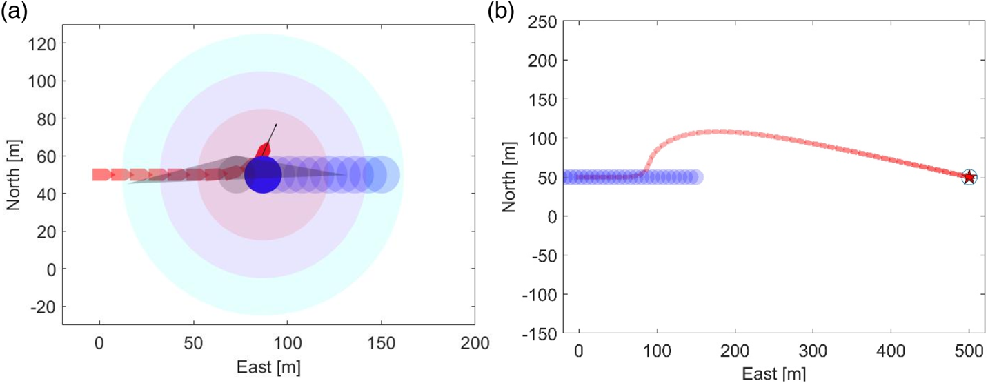
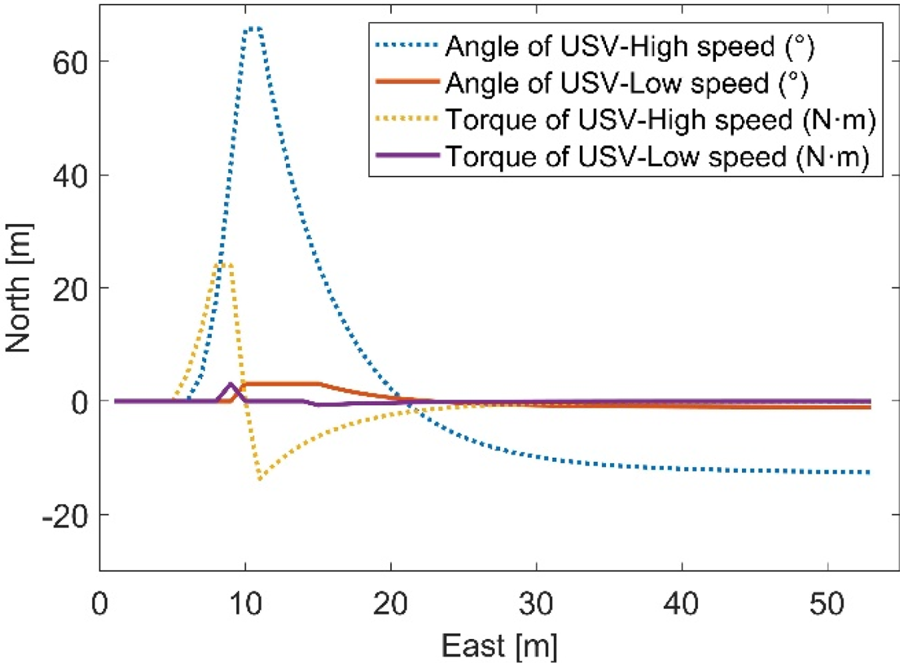
The initial speed of the USV is (10, 0), the initial speed of the obstacle is (−7, 0). It is obvious that they are sailing on the same route. Since the two boats are running at high speed, the end point of v A does not escape the ACC after passing through the pre-avoidance layer and the normal avoidance layer, which leads to the USV entering the emergency layer, then the end point of v A escapes the ACC under the impact of repulsive force. The USV is then set to the velocity locking state, as shown in Figure 9(a). The tracks are shown in Figure 9(b). As shown in Figure 10, the heading angle changes more gently in the low speed encounter scene, while the angular velocity increases faster in the high speed encounter scene. It can be seen from the above simulation that the algorithm shows good collision avoidance performance at different speeds.
The whole process of collision avoidance at high speed: (a) step 10, (b) track of the whole process.

Heading angle and torque.

5.2. Common emergency situation
The actual navigation environment is changing rapidly. In this section, we verify the effectiveness of the algorithm in dealing with an emergency situation.
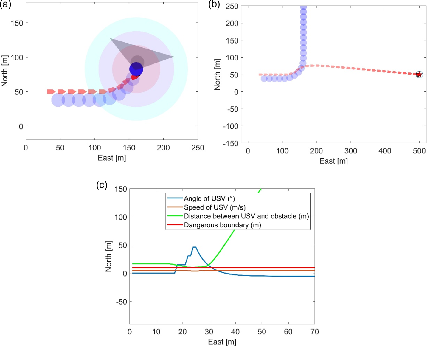
5.2.1. Emergency scenario 1: The obstacle boat turns sharply at close range
The initial position of the USV is (30, 50) and the speed is 5 m/s. The initial position of the obstacle boat is (42, 38), the speed is 5 m/s. Their initial heading angles are the same. The USV is in the free navigating state. Then the obstacle boat suddenly turns left, the USV changes its speed and heading angle under the impact of repulsive force, and the USV passes behind the obstacle boat, as shown in Figure 11(a). The track is shown in Figure 11(b). The heading angle and distance are shown in Figure 11(c).
The whole process of emergency scenario 1: (a) step 29, (b) track of the whole process, (c) the distance, speed and heading angle.

5.2.2. Emergency scenario 2: Two boats meet passing an island
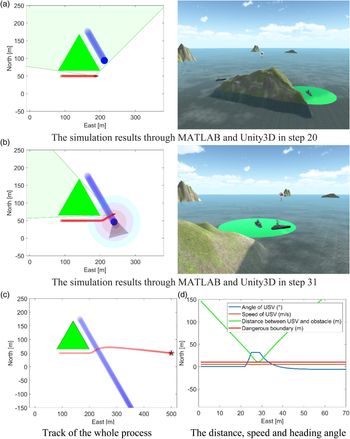
When the USV is navigating past the island (green triangle), the electromagnetic waves from its radar are blocked by the island; the green shaded area is the blind spot of radar. The initial state of the USV is free navigating, as shown in Figure 12(a). A 3D navigation environment is established in Unity. When the USV reaches the intersection (step 22), it suddenly detects an obstacle boat from the port side, it decelerates and turns left; the USV enters the emergency avoidance layer. Under the action of repulsive force, the end point of v A leaves the ACC, then the USV is set to velocity locking state, as shown in Figure 12(b). When the USV starts to move away from the obstacle boat, the locking state is cancelled, as shown in Figure 12(c). The velocity and angular velocity of USV are relatively gentle, as shown in Figure 12(d).
The whole process of emergency scenario 2: (a) simulation results through MATLAB and Unity3D in step 20, (b) simulation results through MATLAB and Unity3D in step 31, (c) track of the whole process, (d) distance, speed and heading angle.

The collision avoidance is realised by a small deceleration action in the emergency situations, which shows a good energy economy.
5.3. Contrast verification
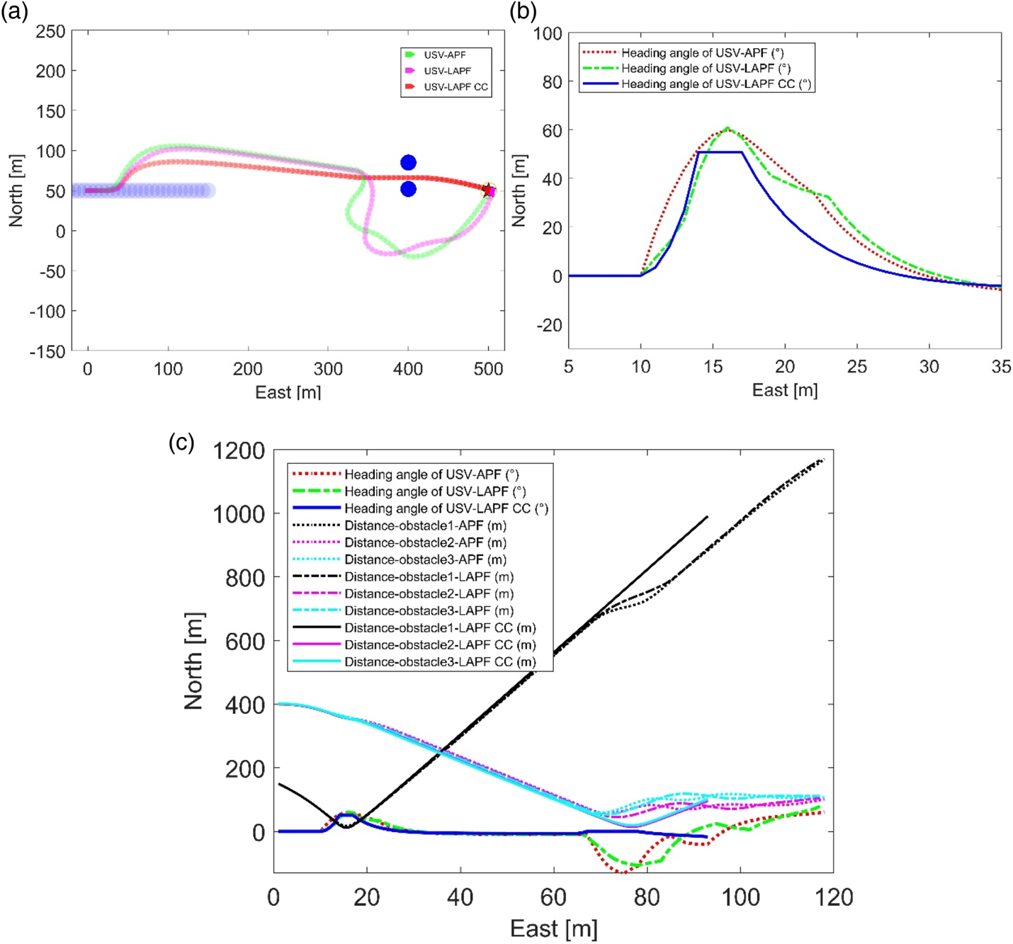
In this section, the APF, LAPF and LAPF-CC methods are compared. Dynamic and static obstacles are set up in the environment. It can be seen from Figure 13(b) that when the USV enters the influence boundary of the repulsive field for the obstacle, it will be affected in the APF algorithm. The heading angle changes suddenly. In the LAPF, the angular velocity is relatively gentle compared with the APF algorithm. The LAPF-CC algorithm has the smallest turning range.
Contrast verification for three algorithms: (a) collision avoidance path, (b) local enlarged drawing of heading angle for avoiding dynamic obstacle, (c) heading angle and distance.

Two static obstacles (blue circles) are set on both sides of the route. Since the LAPF-CC algorithm has the detection ability for collision, the USV is not affected and it can navigate through the middle of the two obstacles and reach the target safely. It can be seen from Figure 13(c) that the LAPF-CC algorithm has the ability to avoid obstacles more narrowly than the other two algorithms.
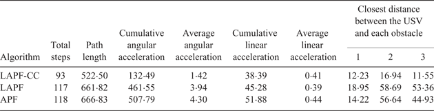
In Table 5, the LAPF-CC algorithm has the fewest total steps, and its path length is 21·64% shorter than that of APF. The LAPF-CC algorithm obtained the best results in terms of cumulative angular acceleration, average angular acceleration and cumulative linear acceleration. With the LAPF-CC algorithm, the USV has the ability to avoid a collision safely in a short distance. The above comparison shows that the LAPF-CC algorithm can significantly reduce the energy consumption and enhance the control stability of the USV.
Comparison of three algorithms.

5.4. Dynamic avoidance of multiple obstacles
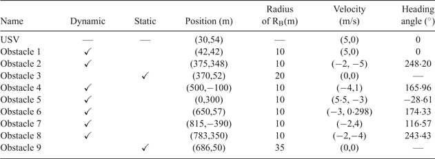
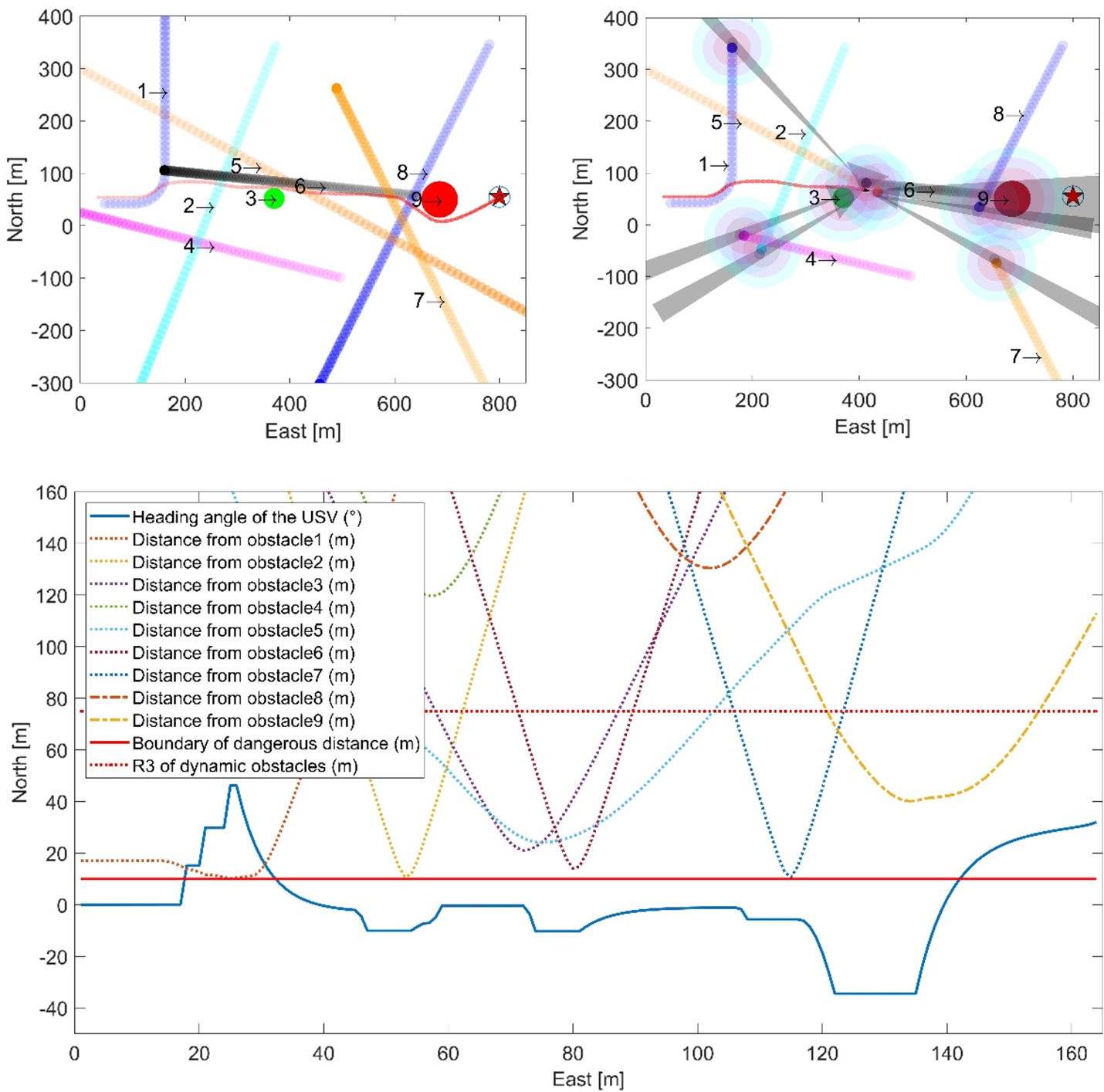
The situation with multiple obstacles is simulated. The initial conditions are shown in Table 6. The total number of simulation steps is 160, the status of the USV and obstacles is output every two steps.
Initial parameters of the USV and the obstacles.

Note:‘—’ means it is not related to the parameter.
The USV is navigating in the same direction as the obstacle boat 1 at the beginning. In step 17, boat 1 suddenly made a sharp turn to the left, which caused the USV to enter the emergency avoidance state. The USV completes the task for collision avoidance in step 24 and successfully passes behind boat 1. The USV then detects boat 2. After the end point of v A escapes from the ACC, the USV enters the velocity locking state in step 47. The USV enters the pre-avoidance layer of obstacle 3 (an island) in step 56, and the velocity locking state is cancelled. v A escapes from the ACC of obstacle 3 in step 59 and the USV enters the velocity locking state. The USV then detects boat 6 approaching head-on. After taking pre-avoidance actions, the USV enters the velocity locking state in step 74 and keeps it until step 80. As shown in Figure 14(c), although the distances between the USV and obstacle 3, boat 5 and boat 6 are very close at this time, the end point of v A does not fall into the ACC of any obstacle, the USV is not affected by their repulsive field. In step 81, the USV begins to move away from boat 6 and enters the free navigating state. Then the USV detects boat 7 coming from starboard; after taking the pre-avoidance actions, the USV enters the velocity locking state in step 108. In step 116, the USV enters the pre-avoidance layer of obstacle 9. After taking actions, the USV does not escape the impact of obstacle 9, and then it enters the normal avoidance layer. The USV escapes from the dangerous area and enters the velocity locking state in step 122. After step 134, the USV begins to move away from obstacle 9. Under the influence of the attractive force of the target, the USV adjusts its heading and finally reaches the target safely.
Dynamic collision avoidance of multiple obstacles: (a) track of the whole process, (b) collision avoidance in high-risk area, (c) heading angle of the USV and distance from obstacles.

Simulation results show that the USV has the ability to handle sharp turns, port encounters, starboard encounters, head-on encounters, static obstacles, and high hazard situations. It can be seen from Figure 14(c) that the heading angle changes smoothly during the whole process. The locking state improves the safety of the USV over a short distance for collision avoidance, and at the same time it avoids the behavior of detour, which plays an important role in the complex environment with multiple obstacles.
6. CONCLUSION
In this paper, a dynamic collision avoidance algorithm via LAPF-CC is proposed. The potential field is divided into four layers according to the danger of the situation. A collision cone with collision risk assessment capability is introduced, and the potential function model of the LAPF-CC is established. The relative distance and relative velocity are used to establish the model of the risk factors for collision, and then the speed torque is constructed. The driving force and torque of the USV are controlled separately. In order to prevent the relative velocity from causing the USV to enter and leave the collision cone frequently, the locking factor is defined. The switch strategy of navigation state is defined. The simulation results show that the algorithm can overcome the adverse effects of the potential field of unrelated obstacles, and achieve better results in avoiding static and dynamic obstacles, especially in dealing with emergency situations in the navigation process.
This paper explores a new collision avoidance method that realises the application of the APF method in dynamic collision avoidance. The next research direction is to integrate more complex dynamic threats into the function of potential field to deal with complex and changeable dynamic environments.
ACKNOWLEDGEMENTS
The research presented in is paper is partly supported by the National Science Foundation of China (61473183, U1509211, 61627810), and National Key R&D Program of China (2017YFE0128500).