







1. Introduction
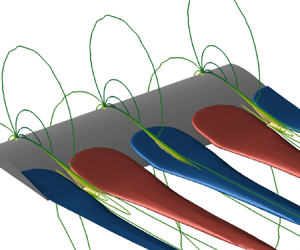
The design of lifting surfaces, such as aeroplane wings, helicopter blades and engine or wind turbine blades, is strongly impacted by the so-called stall phenomenon. It is classically described as the sudden drop of lift that is experienced by the lifting surface when the angle of attack goes beyond a critical value. Appearing for airfoil flows that are characterized by chord-based Reynolds number  ${Re}>10^4$, airfoil stall is associated with the detachment of the laminar or turbulent boundary layer on the suction side of the airfoil, resulting in massive flow separation. The numerical simulation of such high-Reynolds-number flows is still nowadays a challenge when modelling the turbulent flow with the Reynolds-averaged Navier–Stokes (RANS) equations mainly because they are known to fail at reproducing massive flow separation (Spalart Reference Spalart1997). From a more fundamental perspective, there are also complex nonlinear flow phenomena occurring near stalling conditions such as flow hysteresis (Mueller Reference Mueller1985; Hristov & Ansell Reference Hristov and Ansell2018), low-frequency oscillations (Zaman, McKinzie & Rumsey Reference Zaman, McKinzie and Rumsey1989; Broeren & Bragg Reference Broeren and Bragg2001) and three-dimensional stall cells (Winkelman & Barlow Reference Winkelman and Barlow1980; Schewe Reference Schewe2001). This paper aims at investigating the onset of stall cells on an unswept airfoil based on wind-tunnel experimental results, high- and low-fidelity numerical simulations, their merging through data assimilation and global stability analyses.
1.1. Experimental and numerical studies and stability analysis of stall cells
Stall cells, also referred to as owl-faced structures, are three-dimensional cellular patterns that appear on the suction side of airfoils in a narrow range of angles of attack near stalling conditions. Initiated by the flow separation near the trailing edge, stall cells result in a spanwise modulation of the separation line, while the three-dimensional separated flow is organized into counter-rotating vortices concentrating around focal points. Such structures were first observed by Gregory et al. (Reference Gregory, Quincey, O'Reilly and Hall1971) and Moss & Murdin (Reference Moss and Murdin1971) through the use of oil and smoke visualization. In these early experimental studies, the wingspan occupied the entire width of the wind tunnel and the authors suggested that the phenomenon might be caused by the wind tunnel's sidewalls. Later experimental studies performed on finite-aspect-ratio wings with free wing tips by Winkelman & Barlow (Reference Winkelman and Barlow1980) and Schewe (Reference Schewe2001) also reported the formation of stall cells, thus disproving the sidewall effect hypothesis. The wing's aspect ratio still plays a role in the selection of stall cell numbers since they observed that the latter decreases as the aspect ratio of the model decreases. The effects of Reynolds number and wing aspect ratio on the formation of stall cells was investigated by Manolesos & Voutsinas (Reference Manolesos and Voutsinas2013). They showed that the critical angle of attack at which stall cells appear does not depend on the aspect ratio but rather on the airfoil's profile. A linear relationship between the critical angle and the Reynolds number was also established.
Three-dimensional numerical simulations based on RANS models have proven able to capture stall cells. We refer the reader to Manni, Nishino & Delafin (Reference Manni, Nishino and Delafin2016) for a review of early studies performed on several airfoil geometries at chord-based Reynolds number in the range  $3\times 10^4 \leqslant {Re} \leqslant 5\times 10^6$. Those authors specifically investigated the formation of stall cells around a NACA0012 airfoil at
 ${Re}=10^6$ using a large computational domain in the spanwise direction of length
 $L_z=10$ (made non-dimensional with the chord) so as to minimize the influence of the periodic spanwise boundary conditions. For angles of attack
 $17^{\circ } \leqslant \alpha \leqslant 19^{\circ }$, they reported the existence of stall cells characterized by (non-dimensional) spanwise lengths varying in the range
 $1.4 \leqslant \lambda _{z} \leqslant 1.8$ when changing the angle of attack. Liu & Nishino (Reference Liu and Nishino2018) also reported the unsteady behaviour of such stall cells for some angles of attack for the same airfoil. More recently, Plante et al. (Reference Plante, Dandois, Beneddine, Laurendeau and Sipp2021) investigated the formation of stall cells around a NACA4412 airfoil at
 ${Re}=350\,000$ and at
 $\alpha =15^{\circ }$ of size
 $\lambda _{z}=1.5$, considering computational domains with a spanwise extent of
 $L_z=6$ or
 $L_z=12$. While those studies demonstrated the capability of capturing stall cells within the RANS framework, none of them carefully investigated the accuracy of the RANS simulations to determine the onset of stall cells, and in particular the critical angle of attack for a given Reynolds number. One reason is that comparison with results from turbulence-resolving simulations such as large-eddy simulations (LES) or direct numerical simulations (DNS) is still nowadays difficult due to the significant computational cost of these simulations. Indeed, computational domains extending on several chords in the spanwise direction are needed to capture large-scale stall cells while fine grid resolutions are required to resolve the finest flow structures in the turbulent boundary layers. Direct numerical simulations of the turbulent flow around a NACA4412 airfoil at Reynolds number
 $350\,000 \leqslant {Re} \leqslant 400\,000$ have been performed by Hosseini et al. (Reference Hosseini, Vinuesa, Schlatter, Hanifi and Henningson2016) and Gleize, Costes & Mary (Reference Gleize, Costes and Mary2022) with computational domains of short extent in the spanwise direction (
 $L_z=0.1$ and
 $L_z=0.4$, respectively), therefore preventing the appearance of stall cells. More recently, Bouchard et al. (Reference Bouchard, Marty, Deck and Costes2022) performed hybrid RANS/LES simulations of the turbulent flow around an OA209 airfoil at
 ${Re}=10^6$ using a computational domain with
 $L_z=c$ to investigate the dynamics of three-dimensional stall cells. As these studies are very seldom reported in the literature, limits of RANS models in predicting the occurrence of stall cells can be mainly discussed by comparison with experimental results. The first objective of this paper is therefore to identify and characterize deficiencies in RANS modelling that preclude it from accurately capturing the onset of stall cells on a NACA4412 airfoil by comparing experimental and simulation results.
Aside from experimental and direct numerical analyses, the onset of stall has also been investigated through stability analyses. Early theoretical investigations on the physical mechanism for the appearance of stall cells are based on inviscid theory. Weihs & Katz (Reference Weihs and Katz1983) proposed that a Crow instability is responsible for the three-dimensional modulation of the vortex filament associated with the recirculation region on the suction side of the airfoil. Later, Spalart (Reference Spalart2014) derived a simple criterion based on the lifting line theory stating that stall cells appear when the lift curve  $C_{L}(\alpha )$ exhibits a negative slope. Gross, Fasel & Gaster (Reference Gross, Fasel and Gaster2015) also derived a simple formula to determine the wavelength of such stall cells. More recently, Plante, Laurendeau & Dandois (Reference Plante, Laurendeau and Dandois2022) extended such an inviscid analysis using a lifting surface model. At the same time, global stability analyses of two-dimensional steady flows, that are solutions of the Navier–Stokes equations, were successfully applied to identify the existence of three-dimensional stationary global modes in laminar recirculation flows (Theofilis Reference Theofilis2003). Such three-dimensional modes were found to be the primary instability in laminar recirculation flows behind a backward-facing step (Barkley, Gomes & Henderson Reference Barkley, Gomes and Henderson2000; Lanzerstorfer & Kuhlmann Reference Lanzerstorfer and Kuhlmann2012), a bump (Gallaire, Marquillie & Ehrenstein Reference Gallaire, Marquillie and Ehrenstein2007), a curved duct (Marquet et al. Reference Marquet, Lombardi, Chomaz, Sipp and Jacquin2009) or on a flat plate (Rodriguez & Theofilis Reference Rodriguez and Theofilis2010). Based on such encouraging results, Rodríguez & Theofilis (Reference Rodríguez and Theofilis2011) performed a global stability analysis of the flow around a Joukowski airfoil at
 ${Re}=200$ and identified a three-dimensional stationary mode that, once superimposed to the steady flow, gives surface streamlines that are similar to stall cells observed at higher Reynolds numbers. This motivated other studies (Zhang & Samtaney Reference Zhang and Samtaney2016; He et al. Reference He, Gioria, Pérez and Theofilis2017; Nastro et al. Reference Nastro, Robinet, Loiseau, Passaggia and Mazellier2023) on the global stability analysis of airfoil flows at low Reynolds numbers (
 ${Re}\leqslant 1000$). They all showed that this mode is not the primary instability, which is rather a two-dimensional oscillatory mode that leads to the classical von Kármán vortex shedding in the airfoil's wake. To tackle the linear stability analysis of turbulent mean flows for typical values of the Reynolds number
 ${Re}\sim 10^5$ where stall cells are observed experimentally, Plante et al. (Reference Plante, Dandois, Beneddine, Laurendeau and Sipp2021) recently performed a global stability analysis in the framework of the RANS equations. Investigating the turbulent flow around a NACA4412 airfoil at
 $Re = 350\,000$, they showed not only that a three-dimensional stationary mode is the primary instability appearing for
 $\alpha \sim 15^\circ$, but also that its nonlinear evolution leads to the formation of stall cells around the wing. However, global stability analysis performed with RANS equations is likely to suffer from well-known deficiencies of turbulent models in accurately simulating massive flow separation (Spalart Reference Spalart1997), as further discussed in the following.
1.2. Frozen and perturbed eddy-viscosity approaches in linear mean-flow analyses
The reconstruction of coherent fluctuations from linear analysis around a turbulent mean flow has received a lot of attention in the past decade. Most of the recent studies can be classified into three different approaches depending on the considered linearized operator. In the no eddy-viscosity approach (or  $\nu$-model according to Morra et al. (Reference Morra, Semeraro, Henningson and Cossu2019)), the flow variables are simply decomposed into time-averaged and fluctuating components. The exact governing equations for the latter are the linearized Navier–Stokes equations forced by nonlinear terms. In the quasi-laminar stability approach proposed by Mettot, Sipp & Bézard (Reference Mettot, Sipp and Bézard2014), the nonlinear terms are simply neglected and an eigenvalue analysis of the Navier–Stokes operator linearized around the turbulent mean flow is performed to retrieve the turbulent fluctuations. The authors applied such an analysis to reconstruct the low-frequency oscillations in the turbulent wake of a D-shaped cylinder. Instead of neglecting the nonlinear terms, McKeon & Sharma (Reference McKeon and Sharma2010) first proposed to treat them as an exogenous forcing leading to the classical resolvent analysis of the mean flow. The conditions for validity of this linear mean-flow analysis have been discussed by Beneddine et al. (Reference Beneddine, Sipp, Arnault, Dandois and Lesshafft2016) in the case of broadband-frequency turbulent fluctuations developing over a high-Reynolds-number backward-facing step flow. This simple approach is appealing since it is based on the linearized Navier–Stokes operator based solely on the molecular viscosity that can be constructed using mean-flow velocity fields obtained from various numerical simulations (DNS, LES, RANS, etc.). However, it does not discriminate the effects of coherent and non-coherent fluctuations, unlike the two following approaches that are derived from a triple decomposition of the flow variables (Reynolds & Hussain Reference Reynolds and Hussain1972), where fluctuations are further decomposed into the sum of coherent and non-coherent components.
The frozen eddy-viscosity approach is usually derived by considering the exact (but non-closed) governing equations for the coherent fluctuations. While nonlinear interactions between coherent fluctuations are neglected, the effect of the non-coherent fluctuations on the dynamics of the coherent ones is retained by modelling the corresponding Reynolds stress tensor using linear eddy-viscosity models. Such an assumption allows one to simply replace the molecular viscosity of the linearized Navier–Stokes operator with an effective eddy-viscosity field that is the sum of the molecular and turbulent eddy viscosity, hence the name  $\nu _{T}$-model proposed by Morra et al. (Reference Morra, Semeraro, Henningson and Cossu2019). In this approach, the eddy-viscosity field is time-independent, hence the name frozen eddy-viscosity approach. This field may be obtained through several means, such as algebraic models (Reau & Tumin Reference Reau and Tumin2002), more elaborate turbulence models that involve transport equations (Rukes, Paschereit & Oberleithner Reference Rukes, Paschereit and Oberleithner2016), from Reynolds-stress data (Tammisola & Juniper Reference Tammisola and Juniper2016) or through optimization techniques that allow one to retrieve an eddy viscosity that is consistent with the RANS equations (Pickering et al. Reference Pickering, Rigas, Schmidt, Sipp and Colonius2021).
The last and more complex perturbed eddy-viscosity approach is also derived by considering the equations governing the phase-averaged (or ensemble-averaged) component of the flow (defined as the sum of the mean and coherent fluctuations). A phase-averaged eddy-viscosity field can be introduced to express the Reynolds stress tensor as a function of the phase-averaged strain velocity tensor, leading to the (unsteady) RANS equations, which are finally closed by introducing a model for this phase-averaged turbulent eddy viscosity. In this approach, the phase-averaged eddy viscosity is thus decomposed as the sum of time-averaged and infinitesimal coherent fluctuating components, leading to the so-called perturbed eddy-viscosity approach. Crouch, Garbaruk & Magidov (Reference Crouch, Garbaruk and Magidov2007) and Crouch et al. (Reference Crouch, Garbaruk, Magidov and Travin2009) first proposed this approach to predict the onset of transonic buffet on airfoils. Meliga, Pujals & Serre (Reference Meliga, Pujals and Serre2012) considered it to identify the low-frequency oscillations behind a D-shaped cylinder. In both cases, they considered the RANS equations supplemented with the Spalart–Allmaras model (Spalart & Allmaras Reference Spalart and Allmaras1992) to determine the turbulent eddy-viscosity field. The complexity of this perturbed eddy-viscosity approach strongly depends on the complexity of the considered turbulence model. A single supplementary transport equation arises in the linearized operator when considering the one-equation Spalart–Allmaras model, but additional equations would arise if other models were considered such as the  $k$–
 $\omega$ model (Wilcox Reference Wilcox1988). Note that algebraic linear eddy-viscosity models have been considered by Viola et al. (Reference Viola, Iungo, Camarri, Porté-Agel and Gallaire2014) to investigate the coherent fluctuations developing in a wind turbine wake. Such simpler models allow one to reduce the complexity of this approach since the perturbed eddy viscosity can be simply replaced by its analytical expression. The global stability analysis performed by Plante et al. (Reference Plante, Dandois, Beneddine, Laurendeau and Sipp2021) to determine the onset of stall cells around a NACA4412 airfoil belongs to the perturbed eddy-viscosity approach. Not to mention its added complexity, the main drawback of this perturbed eddy-viscosity approach comes from its accuracy. Indeed, as mentioned above, turbulence models are known to have deficiencies in accurately simulating massive flow separation that occurs in particular near stall. As a striking example previously investigated by one of the authors (Busquet et al. Reference Busquet, Marquet, Richez, Juniper and Sipp2021), the global stability analysis of the turbulent flow around an OA209 airfoil near stalling conditions at
 $Re \sim 10^6$ reveals the destabilization of a two-dimensional low-frequency mode at the origin of low-frequency lift oscillation. However, a comparison of the lift coefficient with experimental data showed that the stall angle is overpredicted by a few degrees. Such deficiency in the mean-flow estimation prevents the global stability analysis of baseline RANS equations to quantitatively predict the onset of low-frequency oscillations. For this reason, the no eddy-viscosity and frozen eddy-viscosity approaches are often favoured when mean-flow velocity fields obtained from high-fidelity simulations are available. In the present study, it is shown by comparison with experimental results that the approach of Plante et al. (Reference Plante, Dandois, Beneddine, Laurendeau and Sipp2021) similarly suffers from deficiencies in the underlying turbulence model that prevent it from accurately simulating the mean-flow solution and therefore the onset of stall cells at the correct angle through stability analysis.
1.3. Data assimilation in the RANS framework
The main novelty of the present paper is to propose a systematic method allowing the improvement of the perturbed eddy-viscosity approach. It relies on a better estimation of the mean-flow velocity obtained with a data-consistent RANS model. The latter is defined by introducing a corrective term in the turbulence model that is determined with a data-assimilation method. While data-assimilation methods have a long history of development and application in meteorology and oceanography for reconstructing unsteady flows based on sparse measurements (Kalnay Reference Kalnay2003), such methods have only been recently applied to the reconstruction of time-averaged or (and) spatially averaged flows, also called mean flows. Foures et al. (Reference Foures, Dovetta, Sipp and Schmid2014) used a variational method for estimating the laminar mean flow around a cylinder at Reynolds number  ${Re}=150$. In their approach, a forcing is introduced in the momentum Navier–Stokes equations to mimic the effect of the Reynolds stress tensor induced by the periodic flow fluctuation. This forcing is then determined with an adjoint-based gradient-descent method that aims to minimize the differences between the modelled mean-flow velocity and full (or partial) measurements of a reference mean-flow velocity field. Symon et al. (Reference Symon, Dovetta, McKeon, Sipp and Schmid2017) used a similar methodology to reconstruct the turbulent mean flow around an idealized airfoil at
 ${Re}=13\,500$ using velocity measurements obtained with particle image velocimetry. To overcome the numerical difficulties in solving the time-averaged Navier–Stokes equations at high Reynolds number, Franceschini, Sipp & Marquet (Reference Franceschini, Sipp and Marquet2020) performed the data assimilation of turbulent mean flow modelled with RANS equations. They investigated corrections of the turbulence model (Spalart & Allmaras Reference Spalart and Allmaras1992) as well as corrections of the Boussinesq assumption to estimate the turbulent mean flow behind a backward-facing step at
 ${Re}\sim 30\,000$. Recently, this variational approach was used by Brenner, Piroozmand & Jenny (Reference Brenner, Piroozmand and Jenny2022) to determine a correction of the eddy-viscosity field deduced from the
 $k$–
 $\epsilon$ turbulence model. Cato et al. (Reference Cato, Volpiani, Mons, Marquet and Sipp2023) investigated and compared several correction strategies for the reconstruction of turbulent mean flows around a periodic hill and in the wake of a square cylinder.
The idea of using data assimilation to infer a mean-flow velocity field and applying a linear analysis around the mean flow to reconstruct flow fluctuations has already been proposed by a few authors in the past, mainly using partial experimental measurements to reconstruct the full mean-flow velocity. To investigate the control of vortex shedding in the wake of a thick plate at Reynolds number  ${Re}\sim 10^4$, Camarri, Trip & Fransson (Reference Camarri, Trip and Fransson2017) used the Navier–Stokes equations including a frozen eddy-viscosity field that was calibrated with time-averaged velocity data from particle image velocimetry. The stability analysis of the reconstructed full mean-flow velocity was then performed with the frozen eddy-viscosity approach and substantially improved the estimation of the frequency of the vortex-shedding mode. Symon, Sipp & McKeon (Reference Symon, Sipp and McKeon2019) investigated the flow fluctuations around a NACA0018 airfoil at Reynolds number
 $Re=10^4$ and two angles of attack
 $\alpha =0^{\circ }$ and
 $\alpha =10^{\circ }$. The approach was similar to that proposed by Camarri et al. (Reference Camarri, Trip and Fransson2017) but a forcing vector representing the effect of the Reynolds stress tensor on the mean flow was inferred by data assimilation. A resolvent analysis (McKeon & Sharma Reference McKeon and Sharma2010; Sipp & Marquet Reference Sipp and Marquet2013) of the mean flow with the no eddy-viscosity approach was then performed to retrieve the flow fluctuations. None of these studies described the turbulent mean flow with the RANS equations supplemented with a turbulence model. Very recently, Mons, Vervynck & Marquet (Reference Mons, Vervynck and Marquet2024) used particle image velocimetry data to calibrate a correction of the turbulence model supplementing the RANS equations. With a resolvent analysis performed around the assimilated mean flow in the perturbed eddy-viscosity approach, they successfully predicted the two-dimensional low-frequency oscillation that was observed experimentally around an airfoil at
 ${Re}\simeq 5 \times 10^4$ near stalling conditions.
1.4. Objectives and outline
In this paper, we develop a similar two-fold strategy that is applied to the prediction of stall cells around a NACA4412 airfoil at Reynolds number  $Re = 3.5 \times 10^5$ (Plante, Dandois & Laurendeau Reference Plante, Dandois and Laurendeau2020). Firstly, an adjoint-based data-assimilation method is proposed to correct the baseline RANS model and improve the estimation of mean flows using high-fidelity data that are extracted from DNS (Gleize et al. Reference Gleize, Costes and Mary2022). Several corrections to the turbulence model are considered to improve the mean-flow estimation. Secondly, the temporal evolution of three-dimensional coherent perturbations around the thus-obtained improved mean flows and model is investigated based on global stability analysis and considering frozen and perturbed eddy-viscosity approaches. Results of these stability analyses are assessed through comparison with results of wind-tunnel experiments that are also described in this paper. The paper is organized as follows. The theoretical formulation is detailed in § 2 where we introduce the baseline RANS model, the data-assimilation method with the investigated corrections to the turbulence model and the various approaches (frozen and perturbed eddy viscosity) for global stability analysis around turbulent mean flows. The experimental characterization is described in § 3 where experimental results are compared with those obtained with the baseline RANS model and DNS. Finally, results of mean-flow data assimilation and stability analyses around assimilated mean flows are detailed in § 4. This section includes an assessment of the residual error in the mean-flow velocity obtained with data assimilation and its impact on the stability analysis results based on sensitivity analysis to base flow modifications. It ends with a discussion on the effect of the various corrections of the turbulence model on the results of the stability analysis.
2. Theoretical formulation
2.1. Triple decomposition and closed equations governing the coherent flow
The flow is described by the three-dimensional instantaneous velocity  $\boldsymbol {u}=(u,v,w)^{\rm T}$ and pressure
 $p$ fields that satisfy the non-dimensional incompressible Navier–Stokes equations:
 \begin{equation} \partial_t \boldsymbol{u} + \boldsymbol{\nabla} \boldsymbol{\cdot} \left( \boldsymbol{u} \otimes \boldsymbol{u} \right) + \boldsymbol{\nabla} p - \frac{2}{Re} \boldsymbol{\nabla} \boldsymbol{\cdot} \boldsymbol{S}(\boldsymbol{u}) = \boldsymbol{0} ,\quad \boldsymbol{\nabla}\boldsymbol{\cdot} \boldsymbol{u} = 0, \end{equation}
where  $\boldsymbol {\nabla }=(\partial _x,\partial _y,\partial _z)^{\rm T}$ and
 $\boldsymbol {S}(\boldsymbol {u})$ is the strain rate tensor. The Reynolds number is here defined as
 ${Re}=u_{\infty } c / \nu$, where
 $c$ and
 $u_{\infty }$ are characteristic length and velocity for the specific configuration considered. They are used to make the above velocity and pressure fields non-dimensional. Equations (2.1a,b) are exact but computing their solution requires heavy computational resources when considering turbulent flow configurations. As an alternative to directly solving (2.1a,b), the flow variables can be decomposed according to the triple decomposition (Reynolds & Hussain Reference Reynolds and Hussain1972), which is written for the velocity field as
 \begin{equation} \boldsymbol{u} = \left\langle \boldsymbol{u}\right\rangle+\boldsymbol{u}'' , \quad \left\langle \boldsymbol{u}\right\rangle = \boldsymbol{\bar{u}}+ \boldsymbol{u}', \end{equation}
where  $\left \langle \cdot \right \rangle$ refers to a phase or ensemble average that allows one to extract the coherent part of the flow, while
 $(\cdot )''$ denotes the remaining non-coherent, turbulent part. The coherent part may be further decomposed as the sum of a steady component that is obtained by time-averaging
 $\bar {\cdot }$ and an unsteady coherent fluctuation denoted by
 $\boldsymbol {u}'$. By introducing the above decomposition into the Navier–Stokes equations (2.1a,b) and taking the ensemble average of the latter, we obtain the following exact governing equations for the coherent component of the flow:
 \begin{equation} \left.\begin{gathered}\partial_t \left\langle \boldsymbol{u}\right\rangle + \boldsymbol{\nabla} \boldsymbol{\cdot} \left( \left\langle \boldsymbol{u}\right\rangle \otimes \left\langle \boldsymbol{u}\right\rangle \right) + \boldsymbol{\nabla} \left\langle p \right\rangle - \frac{2}{Re} \boldsymbol{\nabla} \boldsymbol{\cdot} \boldsymbol{S}(\left\langle \boldsymbol{u}\right\rangle ) ={-} \boldsymbol{\nabla} \boldsymbol{\cdot} \left\langle \boldsymbol{u}'' \otimes \boldsymbol{u}'' \right\rangle , \\ \boldsymbol{\nabla}\boldsymbol{\cdot}\left\langle \boldsymbol{u} \right\rangle = 0, \end{gathered}\right\} \end{equation}
where  $\left \langle \boldsymbol {u}'' \otimes \boldsymbol {u}'' \right \rangle$ refers to the Reynolds stress tensor. To obtain a closed set of equations for the coherent part of the flow, we first assume that the anisotropic part of the Reynolds stress tensor
 $\boldsymbol {R}^{a}$ is linearly proportional to the mean strain rate tensor according to
 \begin{equation} \boldsymbol{R}^{a}=\left\langle \boldsymbol{u}'' \otimes \boldsymbol{u}'' \right\rangle - \tfrac{2}{3} k \boldsymbol{I}={-}2 \left\langle \nu_{t}\right\rangle \boldsymbol{S}(\left\langle \boldsymbol{u}\right\rangle ), \end{equation}
where  $k$ and
 $\left \langle \nu _{t}\right \rangle$ are the turbulent kinetic energy and eddy-viscosity fields, respectively. Introducing the Boussinesq approximation into the exact equations (2.3), we obtain
 \begin{equation} \partial_t \left\langle \boldsymbol{u}\right\rangle + \boldsymbol{R}_{\boldsymbol{u}}( \left\langle \boldsymbol{u}\right\rangle , \left\langle P \right\rangle , \left\langle \nu_t \right\rangle ) = \boldsymbol{0} ,\quad \boldsymbol{\nabla}\boldsymbol{\cdot} \left\langle \boldsymbol{u} \right\rangle = 0, \end{equation}
where the momentum residual  $\boldsymbol {R}_{\boldsymbol {u}}$ of the RANS equations is defined as
 \begin{equation} \boldsymbol{R}_{\boldsymbol{u}}( \left\langle \boldsymbol{u}\right\rangle , \left\langle P \right\rangle , \left\langle \nu_t \right\rangle ) = \boldsymbol{\nabla} \boldsymbol{\cdot} \left( \left\langle \boldsymbol{u}\right\rangle \otimes \left\langle \boldsymbol{u}\right\rangle \right) + \boldsymbol{\nabla} \left\langle P \right\rangle - \boldsymbol{\nabla} \boldsymbol{\cdot} \left[ 2 \left( \frac{1}{Re} + \left\langle \nu_t \right\rangle \right) \boldsymbol{S}(\left\langle \boldsymbol{u}\right\rangle ) \right]. \end{equation}
This residual vector is similar to the Navier–Stokes one, except for the molecular viscosity  $1/Re$ which is replaced by the effective eddy-viscosity field
 $(1/Re+\left \langle \nu _t \right \rangle )$. Note that the definition of the pressure is also modified as
 $\left \langle P \right \rangle =\left \langle p \right \rangle +\frac {2}{3}k$. The turbulent eddy viscosity
 $\left \langle \nu _t \right \rangle$ is then determined with a turbulence model. In previous studies about linear analysis around turbulent flows such as that of Viola et al. (Reference Viola, Iungo, Camarri, Porté-Agel and Gallaire2014), algebraic turbulence models (Prandtl's mixing length) have been considered, allowing easy computation of the eddy viscosity from the flow variables. However, such models do not account for history effects on the turbulence, such as convection and diffusion of turbulence kinetic energy. More elaborate models relying on the transport of one or several turbulent variables have been proposed to account for such effects in turbulent flows around airfoils. In the following, we derive the formalism for any one-equation turbulence model (Spalart & Allmaras Reference Spalart and Allmaras1992; Fares & Schröder Reference Fares and Schröder2005; Han, Rahman & Agarwal Reference Han, Rahman and Agarwal2018). We use in §§ 3 and 4 the classical Spalart–Allmaras turbulence model (Spalart & Allmaras Reference Spalart and Allmaras1992) to compute the turbulent eddy viscosity around the present airfoil flow configuration. Note that the methodology is not restricted to one-equation turbulent models. Considering two-equation turbulence models such as the
 $k$–
 $\omega$ model (Wilcox Reference Wilcox1988) is feasible but more tedious and out of the scope of the present paper. Now, any one-equation turbulence model is based on the transport of a turbulent quantity, denoted here
 $\tilde {\nu }$, that is a scalar field related to the turbulent eddy viscosity
 $\left \langle \nu _{t} \right \rangle$ by an analytical relation of the form
 \begin{equation} \left\langle \nu_{t} \right\rangle = f_{\nu_t} (\left\langle \tilde{\nu} \right\rangle ), \end{equation}
where the definition of the function  $f_{\nu _t}$ depends on the considered one-equation model. The latter can be generally written as a transport equation for the turbulent field
 $\tilde {\nu }$ as
 \begin{equation} \partial_{t} \left\langle \tilde{\nu} \right\rangle + T \left( \left\langle \boldsymbol{u}\right\rangle ,\left\langle \tilde{\nu} \right\rangle \right) = \left\langle\,f_n \right\rangle , \end{equation}
where the nonlinear operator  $T( \left \langle \boldsymbol {u}\right \rangle,\left \langle \tilde {\nu } \right \rangle )$ defines the one-equation turbulence model. The latter is specified for the employed Spalart–Allmaras model in Appendix A. All of the existing one-equation turbulence models suffer from deficiencies leading to poor estimation of the coherent velocity
 $\left \langle \boldsymbol {u}\right \rangle$, in particular for massively separated turbulent flows. To address the limitations of the turbulence model and improve the estimation of the coherent component, we follow Parish & Duraisamy (Reference Parish and Duraisamy2016), Singh & Duraisamy (Reference Singh and Duraisamy2016) and Franceschini et al. (Reference Franceschini, Sipp and Marquet2020) by introducing a corrective term in the turbulence model. Several corrections have been proposed in the literature and we refer the reader to Cato et al. (Reference Cato, Volpiani, Mons, Marquet and Sipp2023) for a comparison between these different corrections. For the flow configuration investigated in the present study, the laminar–turbulence flow transition is triggered at some specific locations on the pressure and suction sides of the airfoil. The correction field
 $\left \langle\,f_n \right \rangle$ is chosen as a multiplicative correction term to prevent the appearance of non-zero corrections in the laminar flow regions. The determination of this spatially dependent correction is explained in § 2.3.
2.2. Three-dimensional perturbation of two-dimensional mean flow
The coherent part of the turbulent flow is governed by the closed set of (2.5a,b), (2.6), (2.7) and (2.8). For the three-dimensional turbulent flow around the two-dimensional airfoil considered in the present study, Plante et al. (Reference Plante, Dandois, Beneddine, Laurendeau and Sipp2021) showed that cellular patterns exhibiting a modulation in transverse direction  $z$ are visible in time-independent three-dimensional solutions of this closed set of equations, considering the uncorrected Spalart–Allmaras model (
 $\left \langle g \right \rangle =0$). Rather than solving these three-dimensional equations, we rely on a linearized approach that is more computationally tractable. Since the transverse direction
 $z$ is a homogeneous direction, the average operator
 $\bar {\cdot }$ can be here defined as
 \begin{equation} \overline{({\cdot})}(\boldsymbol{x}) = \frac{1}{T} \frac{1}{L_z} \int_{0}^{L_z} \int_{t_0}^{t_0+T} (\cdot)(\boldsymbol{x},z,t) \,{\rm d}z \, {\rm d}t, \end{equation}
where  $\boldsymbol {x}=(x,y)^{\textrm {T}}$ corresponds to the two-dimensional coordinate while the length
 $L_z$ and time
 $T$ that are used for averaging are specified later. The decomposition (2.1a,b) of the coherent part as the sum of steady and coherent fluctuations can thus be more specifically written as
 \begin{equation} \left.\begin{gathered}
\left\langle \boldsymbol{u}\right\rangle
(\boldsymbol{x},z,t)=\boldsymbol{\bar{u}}(\boldsymbol{x})+
\epsilon \boldsymbol{u}'(\boldsymbol{x},z,t) , \quad
\left\langle P \right\rangle (\boldsymbol{x},z,t) =
\bar{P}(\boldsymbol{x})+ \epsilon p'(\boldsymbol{x},z,t),
\\ \left\langle \tilde{\nu} \right\rangle
(\boldsymbol{x},z,t) = \bar{\nu}(\boldsymbol{x})+ \epsilon
\nu'(\boldsymbol{x},z,t) , \end{gathered}\right\}
\end{equation}
where  $\boldsymbol {\bar {u}}=(\bar {u},\bar {v},0)^{\textrm {T}}$,
 $\bar {P}$ and
 $\bar {\nu }$ are the velocity, pressure and eddy viscosity of the two-dimensional mean flow, while
 $\boldsymbol {u}'(\boldsymbol {x},z,t)$,
 $p'(\boldsymbol {x},z,t)$ and
 $\nu '(\boldsymbol {x},z,t)$ denote the three-dimensional perturbations of the velocity, pressure and eddy-viscosity fields. Moreover, we assume that the amplitude of these perturbations is infinitesimally small, i.e.
 $\epsilon \ll 1$. By introducing the above decomposition (2.10) into the three-dimensional equations (2.5a,b), (2.6), (2.7) and (2.8), we obtain at leading order the time-independent two-dimensional mean-flow equations where the correction is found by a data-assimilation method as explained in § 2.3. At order
 $\epsilon$, we obtain the linearized equations governing the temporal evolution of the three-dimensional perturbations, which are detailed in § 2.4.
2.3. Data-consistent two-dimensional mean-flow equations
The steady two-dimensional equations governing the turbulent mean flow are
 \begin{equation} \boldsymbol{R}_{\boldsymbol{u}}^{0}( \boldsymbol{\bar{u}} , \bar{P}, \bar{\nu}_t ) = \boldsymbol{0} ,\quad \boldsymbol{\nabla} \boldsymbol{\cdot} \boldsymbol{\bar{u}} = 0 ,\quad \bar{ \nu}_{t} = f_{\nu_t} (\bar{\nu} ) ,\quad T^{0} \left( \boldsymbol{\bar{u}},\bar{\nu} \right) = \bar{f}_{n}, \end{equation}
where the two-dimensional residual RANS  $\boldsymbol {R}_{\boldsymbol {u}}^{0}$ and Spalart–Allmaras turbulent model
 $T^{0}$ are defined in (B1) of Appendix B. The effective correction field
 $\bar {f}_n(\boldsymbol {x})$ introduced in the turbulence model is defined as a multiplicative source term, i.e.
 \begin{equation} \bar{f}_n(\boldsymbol{x}) = \bar{\nu}^{n} \bar{g}_{n}, \end{equation}
where  $\bar {g}_{n}(\boldsymbol {x})$ is the corrective field determined by data assimilation and
 $n$ is here a positive integer. For
 $n=0$, we retrieve the correction
 $\bar {f}_{0}=\bar {g}_{0}$ introduced by Franceschini et al. (Reference Franceschini, Sipp and Marquet2020) to correct the fully turbulent mean flow over a backward-facing step. For
 $n>0$, the effective correction
 $\bar {f}_{n}$ will tend to vanish in laminar flow regions since the eddy-viscosity variable
 $\bar {\nu }$ tends towards zero in those regions. More specifically, the correction
 $\bar {f}_2 = \bar {\nu }^2 \bar {g}_{2}$ was recently proposed by Mons et al. (Reference Mons, Vervynck and Marquet2024) to correct the mean-flow velocity around an airfoil near stalling conditions at Reynolds number
 ${Re}\simeq 5 \times 10^4$. For such a flow configuration, the laminar–turbulent flow transition occurs naturally in a laminar separation bubble. To avoid introducing correction of the turbulence model in laminar or transitional flow regions, they introduced the multiplicative correction
 $\bar {f}_{2}$. In the present study dedicated to the turbulent flow around an airfoil where the laminar–turbulence transition is triggered at some specific locations, we additionally investigate the effective corrective field
 $\bar {f}_1 = \bar {\nu } \bar {g}_{1}$ and compare results obtained with these different corrections.
The objective of the data-assimilation method is to determine the two-dimensional correction  $\bar {g}_{n}(\boldsymbol {x})$ that allows one to minimize the differences between the solution of the RANS equations (2.11a–d) and reference data. In the present study, these reference data are time-independent two-dimensional velocity fields
 $\boldsymbol {\bar {u}}_{d}(\boldsymbol {x})$. They are obtained by applying first the average operator (2.9) to three-dimensional instantaneous velocity fields
 $\boldsymbol {u}_{\tiny {DNS}}(\boldsymbol {x},z,t)$ that are computed with DNS (Gleize et al. Reference Gleize, Costes and Mary2022) and, in a second step, a projection operator
 $\mathcal {P}$, further detailed in § 3.3, that maps the space of the DNS to the space of the RANS model. The reference data
 $\boldsymbol {\bar {u}}_d = \mathcal {P} \overline {\boldsymbol {u}_{\tiny {DNS}}}$ are thus defined in the model space. In a least-squares variational framework, the correction
 $\bar {g}_{n}$ is determined by minimizing the following objective function
 $\mathcal {J}$, which is defined as the sum of a data term
 $\mathcal {J}^{u}$ and a penalization term
 $\mathcal {J}^{g_{n}}$:
 \begin{equation} \mathcal{J}(\boldsymbol{\bar{u}}(\bar{g}_{n}))= \underbrace{\int_{\varOmega_m} \left( \boldsymbol{\bar{u}}(\bar{g}_{n}) - \boldsymbol{\bar{u}}_{d} \right)\boldsymbol{\cdot} \left( \boldsymbol{\bar{u}}(\bar{g}_{n}) - \boldsymbol{\bar{u}}_{d} \right) {\rm d}\varOmega}_{\mathcal{J}^{u}} + m \underbrace{\int_{\varOmega} \bar{g}_{n}^2 \,{\rm d}\varOmega}_{\mathcal{J}^{g_{n}}} , \end{equation}
where  $\boldsymbol {\bar {u}}(\bar {g}_{n})$ is a short notation used to indicate that the mean-flow velocity is a solution of the corrected mean-flow equations (2.11a–d). The data term
 $\mathcal {J}^{u}$ is thus the primary objective to minimize in the data-assimilation procedure. It quantifies the discrepancies between the velocity field
 $\boldsymbol {\bar {u}}(\bar {g}_n)$ and the reference one
 $\boldsymbol {\bar {u}}_{d}$ in the restricted domain
 $\varOmega _{m}$ that is part of the computation domain
 $\varOmega$ where (2.11a–d) are satisfied. These domains are specified in §§ 3.2 and 4.1. Note that, since the reference data are in the model space as explained above, we do not introduce a measurement operator in the definition of
 $\mathcal {J}^{u}$ as classically done when the dimensions of the data and model spaces are different. In order to avoid overfitting and restrict the intensity of the corrective field
 $\bar {g}_n$, we also consider the addition of the penalty term, denoted
 $\mathcal {J}^{g_n}$ in (2.13), which is weighted by the positive real number
 $m$. A penalization of the effective correction
 $\bar {f}_{n} =\bar {\nu }^{n}\bar {g}_{n}$ may also be considered. In the present study, it did not lead to corrections that are so different from those obtained with the penalization of the correction
 $\bar {g}_{n}$. The latter is thus favoured hereinafter. The benefits of penalization along with the identification of an appropriate value for
 $m$ are illustrated in § 4.1. The minimization of the objective function (2.13) under the constraint (2.11a–d) is performed with an adjoint-based gradient-descent method. The descent direction is the opposite of the gradient of the objective function with respect to the correction
 $\bar {g}_n$. The latter is defined as
 \begin{equation} \frac{{\rm d}\mathcal{J}}{{\rm d}\bar{g}_{n} }= \bar{\nu}^{{\dagger}} \bar{\nu}^{n} + 2 m \bar{g}_{n}, \end{equation}
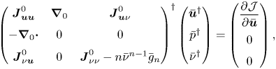
where  $\bar {\nu }^{{\dagger} }$ is the turbulent component of the adjoint variable. The latter is a solution of the following two-dimensional adjoint problem:
 \begin{equation} \left(\begin{array}{@{}ccc@{}} \boldsymbol{J}_{\boldsymbol{u} \boldsymbol{u}}^{0} & \boldsymbol{\nabla}_{0} & \boldsymbol{J}_{\boldsymbol{u} \nu}^{0} \\ -\boldsymbol{\nabla}_{0}\boldsymbol{\cdot} & 0 & 0 \\ \boldsymbol{J}_{\nu \boldsymbol{u}}^{0} & 0 & \boldsymbol{J}_{\nu \nu}^{0} - n \bar{\nu}^{n-1} \bar{g}_{n} \end{array}\right)^{{{\dagger}}} \left(\begin{array}{@{}c@{}} \boldsymbol{\bar{u}}^{{\dagger}} \\ \bar{p}^{{\dagger}} \\ \bar{\nu}^{{\dagger}} \end{array}\right) = \left(\begin{array}{@{}c@{}} \dfrac{\partial \mathcal{J}}{\partial \boldsymbol{\bar{u}}} \\ 0 \\ 0 \end{array} \right) , \end{equation}
where  $(\cdot )^{{\dagger} }$ refers to the adjoint of the operator in (2.15) whose blocks are given in Appendix B. The forcing term (on the right-hand side) of the adjoint RANS equations is the gradient of the objective function with respect to the mean-flow velocity, which is here given by
 \begin{equation} \frac{\partial \mathcal{J} }{\partial \boldsymbol{\bar{u}} } =2 \left( \boldsymbol{\bar{u}} - \boldsymbol{\bar{u}}_{d} \right)\mathbb{1}_{\varOmega_m} . \end{equation}
It is simply the difference between the modelled mean-flow velocity and DNS velocity data in the domain  $\varOmega _{m}$,
 $\mathbb {1}_{\varOmega _m}$ being an indicator function for that domain.
The data-assimilation algorithm is similar to that described by Franceschini et al. (Reference Franceschini, Sipp and Marquet2020), Mons & Marquet (Reference Mons and Marquet2021) and Mons et al. (Reference Mons, Marquet, Leclaire, Cornic and Champagnat2022). We rely on the low-memory Broyden–Fletcher–Goldfarb–Shanno (L-BFGS) descent method (Nocedal Reference Nocedal1980) to perform the minimization of the cost function in (2.13). The latter requires successive inversions of the RANS (2.11a–d) and adjoint (2.15) equations to evaluate the cost function and its gradient in (2.14).
2.4. Linear stability analysis for the identification of coherent perturbations
The linear stability analysis of three-dimensional perturbations to two-dimensional mean flows is now considered, starting with the perturbed eddy-viscosity approach and following with two different frozen eddy-viscosity approaches.
2.4.1. Perturbed eddy-viscosity approach
In the perturbed eddy-viscosity approach, linear perturbations of the eddy viscosity are considered, in addition to the velocity and pressure perturbations, as shown in (2.10). Since the transverse direction  $z$ is homogeneous, the three-dimensional perturbations can be further decomposed as
 \begin{equation} \left.\begin{gathered}\boldsymbol{u}'(\boldsymbol{x},z,t) = \left( \boldsymbol{\hat{u}}(\boldsymbol{x}) {\rm e}^{\lambda t} {\rm e}^{\rm{i} \beta z} + \mbox{c.c.} \right) ,\quad p'(\boldsymbol{x},z,t) = \left( \hat{p}(\boldsymbol{x}) {\rm e}^{\lambda t} {\rm e}^{\rm{i} \beta z} + \mbox{c.c.} \right) ,\\ \tilde{\nu}' (\boldsymbol{x},z,t) = \left( \hat{\nu}(\boldsymbol{x}) {\rm e}^{\lambda t} {\rm e}^{\rm{i} \beta z} + \mbox{c.c.} \right) , \end{gathered}\right\} \end{equation}
where the transverse (real) wavenumber is  $\beta =2{\rm \pi} / \lambda _z$ and
 $\lambda _z$ is the corresponding wavelength. Unlike the discrete approach followed by Plante et al. (Reference Plante, Dandois, Beneddine, Laurendeau and Sipp2021) where values of the wavenumber
 $\beta$ are selected by the length of the computational domain in the transverse direction,
 $\beta$ is here a real parameter that can be arbitrarily chosen since it does not depend on a spatial discretization in the transverse direction. The temporal behaviour is assumed to be exponential with a complex value
 $\lambda = \sigma + \textrm {i}\omega$ that indicates the growth rate
 $\sigma$ (real part) and the frequency
 $\omega$ (imaginary part) of the spatial structure
 $( \boldsymbol {\hat {u}},\hat {p},\hat {\nu })$ that only depends on the two-dimensional coordinate
 $\boldsymbol {x}$. These spatial structures are eigenmodes of the following eigenvalue problem:
 \begin{align} \lambda \left(\begin{array}{@{}ccc@{}} \boldsymbol{I}_{\boldsymbol{u}} & 0 & 0 \\ 0 & 0 & 0 \\ 0 & 0 & 1 \end{array}\right) \left(\begin{array}{@{}c@{}} \boldsymbol{\hat{u}} \\ \hat{p} \\ \hat{\nu} \end{array}\right) + \left(\begin{array}{@{}ccc@{}} \boldsymbol{J}_{\boldsymbol{u} \boldsymbol{u}}^{\beta} & \boldsymbol{\nabla}_{\beta} & \boldsymbol{J}_{u \nu}^{\beta}\\ -\boldsymbol{\nabla}_{\beta}\boldsymbol{\cdot} & 0 & 0 \\ \boldsymbol{J}_{\nu u}^{\beta} & 0 & \boldsymbol{J}_{\nu \nu}^{\beta} - n \bar{\nu}^{n-1} \bar{g}_n \end{array}\right) \left(\begin{array}{@{}c@{}} \boldsymbol{\hat{u}} \\ \hat{p} \\ \hat{\nu} \end{array} \right) = \left( \begin{array}{@{}c@{}} \boldsymbol{0} \\ 0 \\ 0 \end{array} \right), \end{align}
where the velocity vector is defined as  $\boldsymbol {\hat {u}}=(\hat {u},\hat {v},\hat {w})^{\textrm {T}}$ and
 $\boldsymbol {I}_{\boldsymbol {u}}$ is an identity matrix of corresponding size. The other block operators are defined in Appendix B. The first and second lines correspond to the linearization of the RANS equations while the third one corresponds to that of the turbulence model. The linearization of the correction in the turbulence model (2.8) induces the new term
 $-n \bar {\nu }^{n-1} \bar {g}_{n}$ in the
 $(3,3)$ block of the Jacobian matrix in (2.18). For the investigated cases
 $n=1$ and
 $n=2$, the Jacobian matrix is thus structurally modified compared with the baseline model, while for
 $n=0$, this term disappears and the structure of the Jacobian matrix is not altered by the correction of the mean-flow equations. It should be recalled that, whatever the value of
 $n$, the other blocks of the Jacobian matrix are indirectly impacted by the correction. Indeed these blocks correspond to the linearization of the governing equation around the corrected turbulent mean-flow velocity
 $\boldsymbol {\bar {u}}$ and turbulent viscosity
 $\bar {\nu }$, solutions of (2.11a–d). In the present paper, the choice of the correction (i.e the value of
 $n$) is mainly driven by the efficiency of the data-assimilation algorithm to match the reference mean-flow velocity field. The more general impact of the correction term on the results of the stability analysis is discussed in § 4.4 by comparing results obtained with the different corrections
 $n=0$,
 $n=1$ and
 $n=2$. Note finally that the stability analysis around the turbulent mean flow obtained with the baseline turbulence model is simply recovered here by setting
 $\bar {g}_n=0$ in (2.11a–d) and (2.18).
2.4.2. Frozen eddy-viscosity approaches
The frozen eddy-viscosity approach is a simpler analysis that does not require the linearization of a turbulence model. Indeed, the perturbation of the eddy viscosity is neglected  $(\tilde {\nu }'=0)$ and the eigenvalue problem (2.18) is simplified as
 \begin{equation} \lambda\left(\begin{array}{@{}cc@{}} \boldsymbol{I}_{\boldsymbol{u}} & 0 \\ 0 & 0 \end{array} \right)\left(\begin{array}{@{}c@{}} \boldsymbol{\hat{u}} \\ \hat{p} \end{array} \right) + \left(\begin{array}{@{}ccc@{}} \boldsymbol{J}_{\boldsymbol{u} \boldsymbol{u}}^{\beta}(\boldsymbol{\bar{u}},\bar{\nu}) & \boldsymbol{\nabla}_{\beta} \\ -\boldsymbol{\nabla}_{\beta}\boldsymbol{\cdot} & 0 \end{array} \right) \left(\begin{array}{@{}c@{}} \boldsymbol{\hat{u}} \\ \hat{p} \end{array} \right) = \left( \begin{array}{@{}c@{}} \boldsymbol{0} \\ 0 \end{array} \right). \end{equation}
Similarly to the perturbed eddy-viscosity approach, the Jacobian operator  $\boldsymbol {J}_{\boldsymbol {u} \boldsymbol {u}}^{\beta }$ depends on the mean-flow velocity
 $\boldsymbol {\bar {u}}$ and turbulent viscosity
 $\bar {\nu }$ obtained with the data-assimilation method described in § 2.3.
A second frozen eddy-viscosity approach, that does not rely on any data-assimilation process or any turbulence modelling, consists of performing the stability analysis around the reference mean-flow velocity obtained from DNS, i.e.  $\boldsymbol {\bar {u}}_{d}$. To determine a mean eddy viscosity that is consistent with the reference mean-flow velocity, Pickering et al. (Reference Pickering, Rigas, Schmidt, Sipp and Colonius2021) recently proposed a method that is based on the minimization of the RANS residual. This method is revisited in Appendix D. For the second frozen-eddy viscosity approach, the eigenvalue problem can thus be written
 \begin{equation} \lambda \left( \begin{array}{@{}cc@{}} \boldsymbol{I}_{\boldsymbol{u}} & 0 \\ 0 & 0 \end{array}\right) \left(\begin{array}{@{}c@{}} \boldsymbol{\hat{u}} \\ \hat{p} \end{array} \right) + \left(\begin{array}{@{}ccc@{}} \boldsymbol{J}_{\boldsymbol{u} \boldsymbol{u}}^{\beta}(\boldsymbol{\bar{u}}_{d},\bar{\nu}_{t}^{c}) & \boldsymbol{\nabla}_{\beta} \\ -\boldsymbol{\nabla}_{\beta}\boldsymbol{\cdot} & 0 \end{array} \right) \left(\begin{array}{@{}c@{}} \boldsymbol{\hat{u}} \\ \hat{p} \end{array} \right) = \left(\begin{array}{@{}c@{}} \boldsymbol{0} \\ 0 \end{array} \right), \end{equation}
where the Jacobian block operator  $\boldsymbol {J}_{\boldsymbol {u} \boldsymbol {u}}^{\beta }$ now depends on the reference mean-flow velocity
 $\boldsymbol {\bar {u}}_{d}$ and consistent eddy-viscosity field
 $\bar {\nu }_{t}^{c}$, rather than on the assimilated mean flow as in (2.19).
2.5. Sensitivity of eigenvalues to residual error in the assimilated mean-flow velocity
The data-assimilation method described in § 2.3 allows the determination of the correction  $\bar {g}_{n}$ of the turbulent mean-flow equation by minimizing the cost function (2.13). It may be worth noting that the velocity error
 $\delta \boldsymbol {\bar {u}}=\boldsymbol {\bar {u}}_{d}- \boldsymbol {\bar {u}}(\bar {g}_n)$ is not necessarily strictly zero at convergence of the minimization algorithm. We propose here to investigate the uncertainty in the leading eigenvalue that is induced by the uncertainty in the assimilated mean-flow velocity. To that aim, we consider a sensitivity analysis of the eigenvalue to modifications of the mean-flow velocity. Such sensitivity analysis was originally developed for eigenvalues of the Orr–Sommerfeld equations by Bottaro, Corbett & Luchini (Reference Bottaro, Corbett and Luchini2003), later derived by Marquet, Sipp & Jacquin (Reference Marquet, Sipp and Jacquin2008b) for the linearized Navier–Stokes equations and extended by Meliga et al. (Reference Meliga, Pujals and Serre2012) to the RANS equations with the Spalart–Allmaras model. In the latter study, the authors derived the eigenvalue sensitivity to modifications of both velocity and eddy-viscosity mean fields. Here, we restrict ourselves to the sensitivity of the eigenvalue to mean-flow velocity modifications.
Since the residual velocity error  $\delta \boldsymbol {\bar {u}}$ is expected to be small, we consider that it is a small modification of the assimilated mean-flow velocity, i.e.
 $\boldsymbol {\bar {u}} +\delta \boldsymbol {\bar {u}}$, that perturbs the eigenvalue problem (2.18). Following Marquet et al. (Reference Marquet, Sipp and Jacquin2008b) and Meliga et al. (Reference Meliga, Pujals and Serre2012), we can show that the eigenvalue variation
 $\delta \lambda$ that is induced by the mean-flow variation
 $\delta \boldsymbol {\bar {u}}$ is given by
 \begin{equation} \delta \lambda = \int_{\varOmega} \boldsymbol{\nabla}_{\boldsymbol{\bar{u}}} \lambda \boldsymbol{\cdot} \delta \boldsymbol{\bar{u}} \, {\rm d}\varOmega, \end{equation}
where the sensitivity of the eigenvalue  $\lambda$ to mean-flow variations,
 $\boldsymbol {\nabla }_{\boldsymbol {\bar {u}}} \lambda$, is the sum of two contributions:
 \begin{equation} \boldsymbol{\nabla}_{\boldsymbol{\bar{u}}} \lambda = (\boldsymbol{\nabla}_{\boldsymbol{\bar{u}}} \lambda )_{R} + (\boldsymbol{\nabla}_{\boldsymbol{\bar{u}}} \lambda )_{T} . \end{equation}
The first contribution in (2.22), that accounts for the mean-velocity modification in the RANS momentum equations, is defined as
 \begin{equation} (\boldsymbol{\nabla}_{\boldsymbol{\bar{u}}} \lambda )_{R} ={-}( \boldsymbol{\nabla}_{\beta} \boldsymbol{\hat{u}} )^{{\rm T}} \boldsymbol{\hat{u}}^{{\dagger} *} + ( \boldsymbol{\nabla}_{\beta}\boldsymbol{\hat{u}}^{{\dagger} *} ) \boldsymbol{\hat{u}} + \boldsymbol{\nabla}_{0} \boldsymbol{\cdot} \left( \hat{\nu}_{t} (\boldsymbol{\nabla}_{\beta} \boldsymbol{\hat{u}}^{{\dagger} *} + {\boldsymbol{\nabla}_{\beta} \boldsymbol{\hat{u}}^{{\dagger} *}}^{\rm T}) \right), \end{equation}
where we recall that  $\boldsymbol {\hat {u}}$ and
 $\hat {\nu }_{t}$ are the velocity and turbulent eddy viscosity of the direct mode corresponding to the eigenvalue
 $\lambda$ according to (2.18). On the other hand,
 $\boldsymbol {\hat {u}}^{{\dagger} }$ is the velocity component of the adjoint mode, which is a solution of the following eigenvalue problem:
 \begin{equation} \lambda^{*} \left(\begin{array}{@{}ccc@{}} \boldsymbol{I}_{\boldsymbol{u}} & 0 & 0 \\ 0 & 0 & 0 \\ 0 & 0 & 1 \end{array}\right)\left(\begin{array}{@{}c@{}} \boldsymbol{\hat{u}}^{{\dagger}} \\ \hat{p}^{{\dagger}} \\ \hat{\nu}^{{\dagger}} \end{array} \right) +\left(\begin{array}{@{}ccc@{}} \boldsymbol{J}_{\boldsymbol{u} \boldsymbol{u}}^{\beta} & \boldsymbol{\nabla}_{\beta} & \boldsymbol{J}_{u \nu}^{\beta} \\ -\boldsymbol{\nabla}_{\beta}\boldsymbol{\cdot} & 0 & 0 \\ \boldsymbol{J}_{\nu u}^{\beta} & 0 & \boldsymbol{J}_{\nu \nu}^{\beta} - n \bar{\nu}^{n-1} \bar{g}_{n} \end{array} \right)^{{{\dagger}}} \left(\begin{array}{@{}c@{}} \boldsymbol{\hat{u}}^{{\dagger}} \\ \hat{p}^{{\dagger}} \\ \hat{\nu}^{{\dagger}} \end{array} \right) = \left(\begin{array}{@{}c@{}} \boldsymbol{0} \\ 0 \\ 0 \end{array} \right), \end{equation}
where  $(\cdot )^{*}$ denotes complex conjugate. The first two terms on the right-hand side of (2.23) are similar to the sensitivity function for Navier–Stokes equations (Marquet et al. Reference Marquet, Sipp, Chomaz and Jacquin2008a,Reference Marquet, Sipp and Jacquinb), while the last term arises from the added diffusion by the perturbed eddy viscosity. The second contribution on the right-hand side of (2.22) is the eigenvalue sensitivity to mean-velocity modifications in the turbulent model. We refer the reader to Meliga et al. (Reference Meliga, Pujals and Serre2012) for a detailed definition. Once the sensitivity functions are determined, we can assess the variation in the eigenvalue that is induced by the residual mean-flow velocity errors according to (2.21).
2.6. Numerical methods
The two-dimensional mean-flow (2.11a–d) and adjoint (2.15) equations as well as the eigenvalue problems (2.18), (2.19)–(2.20) and (2.24) are spatially discretized using a stabilized Galerkin finite-element method. First, note that the nonlinear terms written in a conservative form in the continuous equations are spatially discretized using a convective form. There are many methods developed over the last 40 years to prevent the appearance of spurious numerical oscillations arising in the simulation of the Navier–Stokes equations at high Reynolds number with classical Galerkin methods. Among the broad class of variational multiscale methods (Hughes et al. Reference Hughes, Feijóo, Mazzei and Quincy1998; Ahmed et al. Reference Ahmed, Chacon Rebollo, John and Rubino2017), we rely here on the classical streamlines upwind Petrov Galerkin (SUPG) method (Tezduyar Reference Tezduyar1991), but other stabilized finite-element methods such as the orthogonal subscale method (Codina Reference Codina2002), the local projection stabilization (Braack & Burman Reference Braack and Burman2006) or the continuous interior penalty method (Burman, Fernández & Hansbo Reference Burman, Fernández and Hansbo2006) could be considered. These methods are mainly developed to overcome some undesirable features of the SUPG methods such as the appearance of artificial boundary conditions on the velocity and pressure or artificial non-symmetric terms (see Burman et al. (Reference Burman, Fernández and Hansbo2006) for others). However, most of these modern stabilized finite-element techniques are applied to the Navier–Stokes equations and not to the RANS equations with turbulence models investigated here. In addition, a recent study by Ahmed & Rubino (Reference Ahmed and Rubino2019) on the simulation of vortex flows at high Reynolds number showed that the accuracy of the standard SUPG method is comparable to that obtained with other stabilization methods. In our formulation, a Grad-Div stabilization term is also included in the discretization of the RANS equations to improve the mass conservation and stabilize the pressure. For the coefficient of the Grad-Div stabilization, we adopt the form proposed by Codina (Reference Codina2000) and also used by Hachem et al. (Reference Hachem, Rivaux, Kloczko, Digonnet and Coupez2010). The Spalart–Allmaras turbulence model is also discretized with the SUPG method as in Sari et al. (Reference Sari, Cremonesi, Khalloufi, Cauneau, Meliga, Mesri and Hachem2018).
An Inf-Sup stable finite-element pair is used to discretize the velocity and pressure fields. Second-order ( $P_2$) Lagrange elements are used for the velocity components while first-order (
 $P_1$) Lagrange elements are used for the pressure and the turbulent viscosity variable. This stabilized finite-element method is implemented in the open-source software FreeFEM (Hecht Reference Hecht2012) using the parallelization strategy based on domain decomposition to assemble the sparse matrices and the interface with the PETSc library (Balay et al. Reference Balay2023) to solve linear problems. We refer the reader to Moulin, Jolivet & Marquet (Reference Moulin, Jolivet and Marquet2019) for a detailed explanation on the parallel implementation of the Navier–Stokes equations in FreeFEM. A quasi-Newton method is implemented to solve the nonlinear RANS equations (2.11a–d). The nonlinear equations are first discretized and then linearized. In particular, all the additional terms arising from the SUPG and Grad-Div stabilization are linearized. The method is viewed as as quasi-Newton method as a real coefficient
 $0 < \gamma \leqslant 1$ is introduced to weight the update field and ensure the convergence of this iterative algorithm. To speed up the latter, a criterion based on the slope of the residual convergence is introduced to avoid the assembly and LU factorization of the Jacobian matrix at each iteration.
To determine dominant eigenvalues that correspond to the largest growth rates in eigenvalue problems such as (2.18), we rely on a shift-and-invert strategy and the Krylov–Schur subspace method implemented in the SLEPc library (Hernandez, Roman & Vidal Reference Hernandez, Roman and Vidal2005). Although the adjoint problems (2.15) and (2.24) are written in a continuous form, their numerical discretization relies on a discrete approach (Peter & Dwight Reference Peter and Dwight2010). The stabilized forms of the direct problems are first implemented and the adjoint matrices are then obtained by taking the transpose (or transconjugate) of the direct matrices. The discrete adjoint is preferred over the continuous adjoint (Papoutsis-Kiachagias & Giannakoglou Reference Papoutsis-Kiachagias and Giannakoglou2016) not only due to its ease of implementation, but also because the eigenvalue spectra of the direct and adjoint matrices are exactly the same. Some numerical artefact might be observed in the adjoint eigenmodes near the inlet of the boundary domain, as discussed by Chandler et al. (Reference Chandler, Juniper, Nichols and Schmid2012), but it did not impact any of the present results.
3. Experimental and numerical characterization of stall cells with the baseline RANS model
We investigate the onset of stall cells around a three-dimensional unswept wing for angles of attack  $\alpha$ near stalling conditions. The constant wing section is a NACA4412 airfoil of chord
 $c=20\ \mathrm {cm}$ and the incoming uniform velocity is close to
 $u_{\infty }= 25 \ \mathrm {m} \mathrm {s}^{-1}$. This characteristic length and velocity are used in the following to make all variables non-dimensional, unless otherwise stated. The air flow is thus characterized by the Reynolds number
 ${Re}=350\,000$ and a low Mach number
 $M<0.1$ so that it is considered as incompressible. For that Reynolds number, the boundary layer developing near the leading edge of the airfoil is laminar. To avoid the formation of any laminar separation bubbles on the suction (upper) side of the airfoil, the laminar–turbulent transition is triggered at chordwise location
 $x^t_{c,u} = 0.05$. On the pressure (lower) side, it is also triggered but further downstream at midchord, i.e.
 $x^t_{c,l} = 0.5$.
The experimental investigation of the onset of stall cells around the wing near stalling conditions is reported in § 3.1. Results of the numerical investigation relying on a baseline RANS model are described in § 3.2, starting by describing the steady mean flow and identifying the critical angle of attack for the appearance of stall cells based on global stability analysis, as in Plante et al. (Reference Plante, Dandois, Beneddine, Laurendeau and Sipp2021). Finally, results of DNS are described and compared with the baseline RANS results in § 3.3.
3.1. Experimental identification of stall cells
Experiments are conducted in the low-speed wind tunnel S2L of ONERA in Chalais-Meudon. The velocity in this Eiffel-type wind tunnel can be varied in the range  $5\ \mathrm {m}\ \mathrm {s}^{-1} \leqslant u_{\infty } \leqslant 40\ \mathrm {m}\ \mathrm {s}^{-1}$. The wing is installed horizontally in the test section so that the wingspan corresponds to the width of the test section. The wingspan made non-dimensional with the chord is thus
 $L_z^{\tiny {exp}} = 4.65$. The transition to turbulence is tripped on the suction and pressure sides of the wing, using zz-shaped ribbons of thickness
 $0.125 \mathrm {mm}$ and length
 $6 \ \mathrm {mm}$ that are positioned along the wingspan at the chordwise locations indicated above, i.e.
 $x^t_{c,u}= 0.05$ and
 $x^t_{c,l} = 0.5$. The wind tunnel's velocity is fixed to
 $u_{\infty } \sim 25\ \mathrm {m}\ \mathrm {s}^{-1}$ so as to obtain a Reynolds number close to
 ${Re}=350\,000$ for air temperature
 $T=10\,^{\circ }\mathrm {C}$. The emergence of structures on the suction side of the wing is characterized using oil visualizations. The oil is a mixture made of paraffin oil, titanium dioxide, oleic acid and blue-coloured pigment. Before any experimental run during which the angle of attack is fixed, this mixture is painted on the entire upper surface of the wing. A camera is located around
 $1\ \mathrm {m}$ above the wing to view its suction side through the glass window that equips the top wall of the test section. During a transient phase, the paint around the leading edge of the wing is driven by the flow towards the trailing edge until a stationary pattern emerges after a few minutes. This pattern approximates the time-averaged wall skin friction over the suction side. In particular, it allows one to distinguish between positive and negative skin-friction areas. Indeed, the paint is almost removed from positive skin-friction areas because it is driven downstream by the flow. Due to the inclination of the wing, gravity also plays a role in driving the paint downstream. On the other hand, in negative skin-friction areas, the paint is driven upstream by the recirculating flow but is counteracted by gravity. Therefore, the paint tends to accumulate in the negative skin-friction area. This accumulation is even more pronounced at the separation line that delimits the negative from positive skin-friction area. The experiments are repeated for each angle of attack which is varied in the range
 $10^{\circ } \leqslant \alpha \leqslant 20^{\circ }$ by steps of
 $1^{\circ }$.
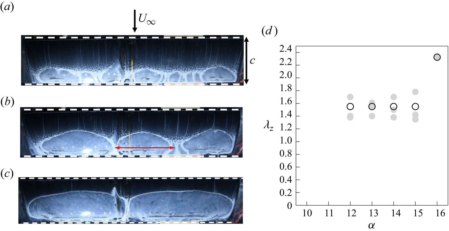
Figures 1(a)–1(c) display typical images acquired during the experimental campaign for angles  $\alpha =10^{\circ }$,
 $12^{\circ }$ and
 $16^{\circ }$. The arrow in figure 1(a) indicates the direction of the incoming flow. The wingspan is thus along the horizontal direction. For angle
 $\alpha = 10^{\circ }$, a spanwise variation of the separation line is visible at the junction of the wing with the sidewalls of the wind tunnel, showing the existence of three-dimensional corner flows. The variation of the separation line is, however, much weaker in the symmetry plane of the test section. Such a pattern, which is not associated with stall cells, is also obtained for all angles below
 $10^{\circ }$. For
 $\alpha = 12^{\circ }$ (figure 1b), a clear spanwise oscillation of the separation line emerges, with three stall cells appearing along the transverse direction. The non-dimensional wavelength of individual stall cells is approximated by considering the ratio between the length of the red arrow displayed in figure 1(b) and the chord of the wing estimated here as the distance between the leading and trailing edges as visible on the images with horizontal dashed lines. This method does not account for the optical distortion of the image. The wavelength of these individual cells is reported with grey circles in figure 1(d) as a function of the angle of attack. It lies in the range
 $1.4 \leqslant \lambda _{z} \leqslant 1.8$ for angles
 $12^{\circ } \leqslant \alpha \leqslant 15^{\circ }$. A unique value of the wavelength, reported with open circles in the figure, can also be obtained by defining
 $\lambda _z= L_z^{\tiny {exp}} / n_{c}$, where
 $n_{c}$ is the number of cells and we recall that
 $L_z^{\tiny {exp}} = 4.65$. Patterns of
 $n_c=3$ cells are observed for
 $12^{\circ } \leqslant \alpha \leqslant 15^{\circ }$, which correspond to the fixed wavelength
 $\lambda _z = 1.55$. Around
 $\alpha = 16^{\circ }$, a transition occurs to a pattern of
 $n_c=2$ cells that is shown in 1(c). For larger values of
 $\alpha$, a clear pattern of stall cells is no longer observed. In conclusion of this experimental investigation, the critical angle of attack for the onset of stall cells is
 $\alpha _{c}^{\tiny {exp}}=12^{\circ }$ with an accuracy of
 $1^{\circ }$ and the wavelength of the corresponding stall cells is
 $\lambda _{z}^{\tiny {exp}}=1.55$.
Experimental evidence of stall cells on the suction side of a NACA4412 wing for  $Re = 350\,000$ using oil flow visualization at (a)
 $\alpha = 10^{\circ }$, (b)
 $\alpha = 12^{\circ }$ and (c)
 $\alpha = 16^{\circ }$ angles of attack. The black arrow in (a) indicates the direction of the incoming flow. Positions of the leading and trailing edges are delimited with horizontal white dashed lines. (d) Non-dimensional wavelength of stall cells
 $\lambda _z$ as a function of the angle of attack. Grey circles show the wavelengths extracted from the images while open black circles indicate the wavelength based on the number
 $n_c$ of observed cells, i.e.
 $\lambda _z = L_z^{\tiny {exp}}/n_c$, where the (non-dimensional) wingspan is
 ${L^{\tiny {exp}}_z=4.65}$.
3.2. Mean flow and global stability analysis with the baseline RANS model
Following an approach similar to that in Plante et al. (Reference Plante, Dandois, Beneddine, Laurendeau and Sipp2021), we here numerically investigate the onset of stall cells on the same NACA4412 airfoil in the same conditions. Neglecting the effect of the sidewalls in the wind-tunnel test section, we may assume that the spanwise direction is a homogeneous direction. Therefore, the mean-flow velocity field around the NACA4412 airfoil can be estimated with the two-dimensional RANS equations, which are here closed with the Spalart–Allmaras model, i.e. (2.11a–d). When the turbulence model is not corrected ( $\bar {g}=0$), this set of equations is referred to as the baseline RANS model. The
 $f_{t2}$ tripping function of the Spalart–Allmaras model (see Appendix A) is used to trigger transition to turbulence at the same locations as in the experiments, i.e.
 $x^t_{c,u} = 0.05$ and
 $x^t_{c,l} = 0.5$ on the suction and pressure sides of the airfoil, respectively.
The mean-flow equations and eigenvalue problems are discretized on a C H computational domain, with the leading edge of the airfoil located at the centre of the half-circle (C) whose radius is  $R=29$. The outlet is located at
 $L_{x}^{o}=30$ of the airfoil's leading edge, while the upper (lower) boundary is located at
 $L_{y}^{u}= 30$ (
 $L_{y}^{l}= 30$). An unstructured mesh made of triangular elements is then obtained with a Delaunay triangulation. The RANS equations (2.11a–d) are spatially discretized on this mesh with the stabilized finite-element method that is described in § 2.6 and using the following boundary conditions. At the inlet, we impose Dirichlet boundary conditions on the non-dimensional velocity, i.e.
 $\bar {u}=\cos (\alpha {\rm \pi}/180),\bar {v}=\sin (\alpha {\rm \pi}/180)$, where
 $\alpha$ is the angle of attack expressed in degrees, while
 $\bar {\nu }=3/ Re$ is set for the eddy-viscosity variable. Therefore, the angle of attack is imposed via the direction of the inlet flow in the numerical simulations. All results are, however, presented in the rotated axis of the coordinates where the inflow velocity is
 $(\bar {u}=1,\bar {v}=0)$ so that the angle of attack is visible on the airfoil position. At the outlet of the computation domain, a stress-free boundary condition is imposed. Finally, symmetry conditions
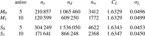
 $\partial _y \bar {u}=0, \bar {v}=0, \partial _y \bar {\nu }=0$ are imposed on the upper and lower lateral boundaries. The eigenvalue problem (2.18) is discretized on the same mesh with boundary conditions corresponding to those imposed for the steady solution. Homogeneous Dirichlet boundary conditions on the velocity and eddy viscosity are imposed on the inlet, upper and lower lateral walls, while the stress-free boundary conditions are also applied at the outlet. Table 1 reports results of mean-flow and eigenvalue computations that are obtained for meshes with different resolutions. The meshes labelled
 $M_0$ and
 $M_1$ are obtained using a metric-based anisotropic mesh adaptation where the parameter aniso (first column) controls the maximum anisotropy (aspect ratio) of the triangles. The metric is computed automatically from mean-flow velocity, pressure and turbulent viscosity fields that are obtained from a preliminary computation. The meshes labelled
 $S_0$ and
 $S_1$ are obtained using a second metric-based anisotropic mesh adaptation, where the metric is now determined from the endogeneity function in addition to the mean-flow solutions that are computed with meshes
 $M_0$ and
 $M_1$, respectively. This endogeneity function, which is introduced later in the paper to identify the flow region where destabilizing physical mechanisms are at play (Marquet & Lesshafft Reference Marquet and Lesshafft2015; Paladini et al. Reference Paladini, Marquet, Sipp, Robinet and Dandois2019), is rather used here to refine the mesh in regions where the direct and adjoint global modes overlap so as to ensure mesh convergence of the stability results, as proposed by Fabre et al. (Reference Fabre, Citro, Ferreira Sabino, Bonnefis, Sierra, Giannetti and Pigou2018). The effect of the mesh resolution on the mean flow is reported by examining the lift coefficient
 $C_L$ that exhibits variations that are lower than
 $0.1\,\%$ among all cases. The effect of the mesh resolution on the eigenvalue problem is reported by examining the growth rate of the leading zero-frequency mode at wavenumber
 $\beta =5$ which will be of interest later. Decreasing the anisotropy coefficient by
 $2$ has also a negligible effect on the growth rate, so the anisotropy coefficient
 $10$ is selected since it leads to coarser meshes. The refinement of the mesh in regions of large endogeneity (meshes
 $S_k$) induces larger variations of the growth rate around
 $10\,\%$ compared with meshes
 $M_k$, showing the interest in adopting this strategy. For the next results, we thus adopt the following mesh adaption procedure for each value of the angle of attack that will be considered, where a mesh of type
 $M_1$ is first built, followed by the construction of a mesh of type
 $S_1$.
Effect of the mesh resolution on mean-flow and global stability analysis results with the baseline RANS model at  $\alpha =16^{\circ }$. Different meshes
 $M_k$ (adapted to mean-flow results only) and
 $S_k$ (adapted to both mean-flow and endogeneity results) are considered that correspond to different values of the parameter aniso that is a measure of the mesh anisotropy, while
 $n_e$ is the number of elements (triangles),
 $n_{d}$ is the total number of degrees of freedom and
 $n_{w}$ is the number of nodes on the airfoil's wall. Parameter
 $C_L$ is the lift coefficient of the mean flow and
 $\sigma _L$ is the growth rate of the leading zero-frequency eigenvalue for
 $\beta =5$.
The streamwise component  $\bar {u}$ of the mean-flow velocity and the turbulent eddy viscosity
 $\bar {\nu }_{t}$ are shown in figures 2(a) and 2(b), respectively, for angle of attack
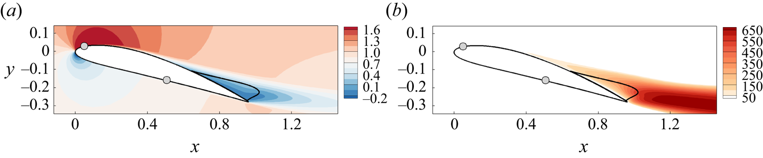
 $\alpha =16^{\circ }$. The grey circles indicate the locations for triggering laminar–turbulent transition. On the pressure side of the airfoil, the boundary layer remains attached. On the suction of the airfoil, the turbulent boundary layer separates at
 $x_{c,u}=0.54$ forming a recirculation region around the trailing edge. An increase of the turbulent eddy-viscosity field is noticeable from the flow separation, with the largest magnitude reached downstream of the recirculation region.
(a) Streamwise velocity  $\bar {u}$ and (b) turbulent eddy viscosity
 $\bar {\nu }_{t}$ normalized by the kinematic viscosity of the baseline RANS model for
 $\alpha =16^{\circ }$. Solid curves are the dividing streamlines of the separated flow at the trailing edge. Grey circles indicate the positions for triggering the laminar–turbulent transition on the upper and lower surfaces.
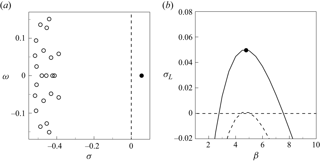
The global stability of this mean flow is investigated by considering the perturbed eddy-viscosity approach described in § 2.4.1. The temporal evolution of linear three-dimensional perturbations is considered for several spanwise wavenumbers  $\beta$. A typical eigenvalue spectrum obtained after solving the eigenvalue problem (2.18) is shown in figure 3(a) for the transverse wavenumber
 $\beta =5$. The horizontal axis corresponds to the growth rate
 $\sigma$ and the vertical axis to angular frequency
 $\omega$ of the eigenmodes. The mean flow is globally unstable since there is a steady eigenvalue (
 $\omega = 0$) emphasized with the black filled circle that has a positive growth rate (
 $\sigma >0$). Its spatial structure, which is analysed in the next section, corresponds to stall cells. Figure 3(b) shows how the growth rate of this leading steady mode, which is denoted by
 $\sigma _{L}$, varies with the wavenumber
 $\beta$. It is unstable in the range
 $4 \leqslant \beta \leqslant 6$ and the maximum growth rate is reached for
 $\beta =4.8$. By repeating the analysis for lower values of the angle of attack, we determine the critical angle to be
 $\alpha _{c}^{\tiny {RANS}}=15.65^{\circ }$ and the critical wavelength
 $\lambda _z^{\tiny {RANS}} = 2 {\rm \pi}/ \beta = 1.30$.
Global stability analysis in the perturbed eddy-viscosity approach of the mean flow estimated with the baseline RANS model at  $\alpha =16^{\circ }$. (a) Eigenvalue spectrum for spanwise wavenumber
 $\beta =5$, with
 $\sigma$ the growth rate and
 $\omega$ the angular frequency. The black filled circle highlights the leading (unstable) eigenvalue. (b) Growth rate
 $\sigma _{L}$ of the leading steady mode versus the wavenumber
 $\beta$ (solid curve). The dashed curve shows the leading eigenvalue growth rate for the critical angle of attack
 $\alpha _c=15.65^{\circ }$.
The global stability analysis of the mean flow around the same NACA4412 airfoil at  ${Re} = 350\,000$ has been recently performed by Plante et al. (Reference Plante, Dandois, Beneddine, Laurendeau and Sipp2021) using a perturbed eddy-viscosity approach of the compressible RANS equations for Mach number
 $M=0.2$. The Spalart–Allmaras turbulence model was also considered but using the modification proposed by Edwards & Chandra (Reference Edwards and Chandra1996). They found that the stall cell mode becomes first unstable at
 $\alpha _{c} \sim 15^{\circ }$ for the wavenumber
 $\beta _c \sim 4.4$ (
 $\lambda _{z} \sim 1.4$). Our results are thus in good agreement with these previously published results for the exact same airfoil, Reynolds number and triggering locations. The slight discrepancies might be attributed either to flow modelling differences, such as the compressibility of the RANS equations or the version of the Spalart–Allmaras turbulent model, or to the different spatial discretization used in the two studies (finite volume versus stabilized finite element). Plante et al. (Reference Plante, Dandois, Beneddine, Laurendeau and Sipp2021) also performed three-dimensional RANS computations using periodicity conditions in the spanwise direction with a wingspan equal to a multiple of the wavelength
 $\lambda _z = 2 {\rm \pi}/ \beta _c$. Thus, they could determine the nonlinear three-dimensional steady solutions that emerge from the linear stall cell mode. These nonlinear solutions exhibited cellular patterns, whose number depends on the wingspan, and which have characteristics of stall cells as reported in previous experiments for other airfoils (Schewe Reference Schewe2001). Thus, they confirmed that the linear stall cell mode is responsible for the emergence of stall cells.
The critical wavelength obtained from linear stability analysis  $\lambda _{z}^{\tiny {RANS}} =1.30$ is in rather good agreement with the wavelength of stall cells
 $\lambda _z^{\tiny {exp}} = 1.55$ observed in the experiments. However, the critical angle of attack
 $\alpha _{c}^{\tiny {exp}}=12^{\circ }$ is much lower than the critical angle of attack
 $\alpha _{c}^{\tiny {RANS}}=15.65^{\circ }$ determined by the stability analysis of the mean flow with the baseline RANS model. To analyse the origin of that discrepancy, we compare in the next section the mean flow estimated using the baseline model with that computed using DNS.
3.3. Comparison with mean flows extracted from DNS
High-fidelity simulations of this transitional turbulent flow were recently performed by Gleize et al. (Reference Gleize, Costes and Mary2022) with the in-house compressible flow solver FastS. The structured mesh is made of  $1.68 \times 10^9$ cells. With the mesh resolution detailed in Gleize et al. (Reference Gleize, Costes and Mary2022), the accuracy of that numerical simulation lies between that of a DNS and of an implicit LES. The authors thus considered that they performed quasi-DNS but we will refer to them as DNS in the following. To trigger the laminar–turbulent transition, small cylindrical roughness elements were equidistantly distributed in the spanwise direction at the same locations as in the experiments on the pressure and suction sides of the airfoil. Hairpin vortex structures are thus generated in the wake of these cylindrical roughness elements, thus leading to a rapid transition to turbulence. Periodic boundary conditions are applied on the side planes of the mesh. Therefore, these simulations do not aim at reproducing the three-dimensional sidewall effect occurring in the experiments. On the other hand, they allow one to accurately determine turbulent flow statistics. For the two angles of attack
 $\alpha =10^{\circ }$ and
 $\alpha = 11^{\circ }$ for which DNS have been performed, it is important to note that the extension of the wing along the span is
 $L_{z}^{\tiny {DNS}}=0.4$ in the simulations. This is much smaller than the experimental wingspan
 $L_{z}^{\tiny {exp}}=4.65$ and too small to observe the stall cells of wavelength
 $\lambda _{z}^{\tiny {exp}}=1.55$. The mean flows that are obtained from DNS can therefore be used as reference for the mean flows estimated with the two-dimensional RANS simulations.
The reference mean-flow velocity data are precisely defined as  $\boldsymbol {\bar {u}}_{d} = \mathcal {P} \bar {\boldsymbol {u}}_{\tiny {DNS}}$ where the unsteady flow solution
 $\boldsymbol {u}_{\tiny {DNS}}$ is first averaged over time and space along the spanwise direction, in accordance with (2.9). Five convective times, excluding initial transients, are used for the time averaging. Secondly, the mean-flow statistics computed on the fine structured grid used for the DNS are then projected onto the coarser unstructured grid used to discretize the RANS equations. This spatial projection, which is defined by the operator
 $\mathcal {P}$, is more precisely composed of two steps. In the first step, a very fine unstructured mesh is obtained by using a Delaunay triangulation from all the points of the fine structured grid used for the DNS. On this fine unstructured mesh, the mean-flow velocity field is discretized with linear Lagrange elements such that all the nodes of the solution correspond exactly to the points of the structured grid used for DNS. Therefore, there is no interpolation error in this first step. In a second step, a coarser unstructured mesh is generated using a Hessian-based mesh adaptation where the metric is computed from the mean-flow velocity and pressure fields. On this coarser unstructured mesh, the mean-flow velocity is discretized with quadratic Lagrange elements. An interpolation from the space spanned by linear Lagrange elements defined on the fine mesh to the space spanned by quadratic Lagrange elements defined on the coarser mesh is finally performed to obtain the reference velocity data
 $\boldsymbol {\bar {u}}_{d}$. Several tests, not reported here, have been performed to ensure that the interpolation errors that arise during this second step are negligible.
The streamwise velocity  $\bar {u}_d$ of the mean flow extracted from DNS is displayed in figures 4(a) and 4(b) for angles
 $\alpha =10^{\circ }$ and
 $\alpha = 11^{\circ }$, respectively. A turbulent trailing-edge separation is observed for both angles of attack, leading to a recirculation region that is delimited with the black solid curve in the figure. The turbulent separation occurs at
 $x_{c,u} = 0.866$ and
 $x_{c,u} = 0.816$ and the maximum back-flow velocities are
 $\bar {u}_d = -0.14$ and
 $\bar {u}_d = - 0.16$ for angles
 $\alpha =10^{\circ }$ and
 $\alpha = 11^{\circ }$, respectively. The turbulent flow separation is similar to that obtained with the baseline RANS model (figure 2a) but at a much larger angle of attack (
 $\alpha =16^{\circ }$). For comparison, the mean-flow velocity fields obtained with the baseline RANS model at the same angles of attack
 $\alpha =10^{\circ }$ and
 $11^{\circ }$ are shown in figures 4(c) and 4(d), respectively. The turbulent boundary layer is now fully attached on the suction side of the airfoil. There is no turbulent separation near the trailing edge, unlike what is observed for the DNS mean flow (figure 4a,b). These discrepancies between baseline RANS and DNS are also apparent when comparing the turbulent eddy viscosity. While the eddy-viscosity field
 $\bar {\nu }_{t}^{{\tiny RANS}}$ is naturally retrieved from the Spalart–Allmaras model, we use the approach described in Appendix D to extract an eddy-viscosity field
 $\bar {\nu }_t^c$ that is consistent with the DNS mean velocity. Figure 5 displays both eddy-viscosity fields for angle
 $\alpha =11^{\circ }$. They are divided by the kinematic viscosity, or, when considering non-dimensional variables, multiplied by the Reynolds number. The DNS-consistent eddy viscosity (figure 5b) is much larger in the wake of the airfoil. This results from the trailing-edge flow separation that induces a larger production of turbulence. That striking discrepancy results from, rather than explains, the inability of the baseline RANS model to capture the turbulent flow separation. We will see in the following that the overproduction of eddy viscosity in the turbulent boundary layer upstream of the flow separation (i.e.
 $x_{c,u} < 0.8$) is responsible for the failure of the baseline RANS model.
Streamwise component of the mean-flow velocity obtained from (a,b) DNS and (c,d) baseline RANS simulations for angles of attack (a,c)  $\alpha =10^{\circ }$ and (b,d)
 $\alpha =11^{\circ }$.

Turbulent eddy viscosity normalized by the kinematic viscosity obtained with (a) baseline RANS ( $\bar {\nu }_{t}^{{\tiny RANS}}$) and (b) DNS (
 $\bar {\nu }_t^c$). The latter is extracted from DNS data as described in Appendix D. The angle of attack is
 $\alpha =11^\circ$.

A comparison between experimental results and numerical results obtained with the baseline RANS model and DNS is reported in figure 6 by displaying the lift coefficient  $C_L$ as a function of the angle of attack. The baseline RANS model (solid curve) clearly overpredicts the lift coefficient obtained from DNS (crosses) and measured experimentally (circles). The latter is obtained by integrating static wall-pressure measurements that are available in the symmetry plane of the wing at several locations on the suction and pressure sides of the airfoil. At angle
 $16^{\circ }$, where the presence of stall cells is predicted by linear stability analysis of the baseline RANS model, the discrepancy in the lift coefficient is around
 $30\,\%$ between RANS and experiments. That discrepancy in the mean-flow solution is associated with an error of
 $4^{\circ }$ in the critical angle
 $\alpha _{c}$ for the onset of stall cells as estimated by baseline RANS, which is clearly visible in the figure. Interestingly, we observe that, for the two angles
 $10^{\circ }$ and
 $11^{\circ }$ where stall cells are not observed in the experiments (open circles), the lift predicted with DNS is close to that measured experimentally. In the next section, the mean-velocity fields obtained from DNS are used as reference data to improve the baseline RANS model and better predict the onset of stall cells with stability analysis.
Time-averaged lift coefficient  $C_L$ as a function of the angle of attack
 $\alpha$ for the baseline RANS model (curves), DNS (crosses) and experiments (circles). Stable and unstable RANS solutions are shown with solid and dashed curves, respectively. Filled and open circles indicate the existence or not of stall cells in the experiments. The critical angles of attack
 $\alpha _{c}^{\tiny {RANS}}=15.68^\circ$ and
 $\alpha _{c}^{\tiny {exp}}=12^\circ$ are also indicated.
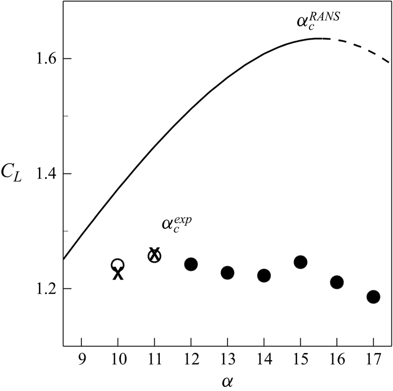
4. Prediction of stall cells based on linear analyses of DNS-consistent mean flows
To improve the prediction of stall cells based on linear stability analysis, we report in § 4.1 results of the data-assimilation method where the baseline RANS model is corrected using the above-discussed reference mean-flow velocity fields from DNS. Linear stability analysis around the assimilated mean flows is then performed in § 4.2 starting with results of the perturbed eddy-viscosity approach. These results are compared not only with experimental results, but also with those obtained with simpler frozen eddy-viscosity approaches. The impact of the residual velocity error in the assimilated mean flow on the stall cell eigenvalue is assessed in § 4.3 using sensitivity analysis. Finally, the influence of the model correction on the stability analysis results is discussed in § 4.4.
4.1. Data-assimilation results
The data-assimilation method introduced in § 2.3 is first applied in § 4.1.1 relying on the correction  $\bar {f}_{1}$ in the turbulence model. The choice of the model correction (
 $\,\bar {f}_{k}$) and its influence on the estimation of the mean-flow velocity are then further investigated in § 4.1.2.
4.1.1. Results with the correction  $\bar {f}_{1}$

The data-assimilation method using the correction  $\bar {f}_{1}=\bar {\nu } \bar {g}_{1}$ in the turbulence model in (2.11a–d) is first applied to the estimation of the mean-flow velocity at
 $\alpha =11^{\circ }$.
We recall that the objective function  $\mathcal {J}$, defined in (2.13), is the sum of two terms. The first term
 $\mathcal {J}^u$ accounts for the velocity error in the domain
 $\varOmega _m$ that is restricted here to
 $-0.5< x<1.5$ and
 $-0.3< y<0.2$. The second term
 $\mathcal {J}^{g_n}$ penalizes the correction field
 $\bar {g}_{n}$ in the full computational domain so as to improve the well-posedness of the minimization problem and also to avoid non-physical large-amplitude correction fields. These two terms are weighted by the penalty parameter
 $m$. The evolution of the two terms defining the cost function is shown in figure 7(a) during the iterative process of the data-assimilation algorithm, for the penalty parameter
 $m=10^{-4}$. The cost function
 $\mathcal {J}$ (dashed curve) decreases by almost two orders of magnitude in
 $100$ iterations. The decrease is sharp during the first
 $20$ iterations and quite slow for the remaining
 $80$ iterations. The velocity error (solid curve) follows the same evolution while the penalization term (dash-dotted curve) increases strongly during the first
 $20$ iterations before stagnating close to a value below
 $10^{-2}$. To better understand the effect of the penalization parameter, figure 7(b) reports the value of the cost function at convergence for several values of the penalty parameter in the space
 $(\mathcal {J}^{u}/\mathcal {J}_{0},\mathcal{J}^{g_n}/\mathcal {J}_{0})$. The arrow indicates increasing values of the penalization parameter indicated in the caption of the figure. For small values of the penalty parameter, the velocity error
 $\mathcal {J}^{u}/\mathcal {J}_{0}$ is around
 $5\times 10^{-3}$, smaller than the velocity error reached in figure 7(a). However, the correction field (not shown here) then exhibits large peaks localized in space that induce strong values of
 $\mathcal{J}^{g_n}/\mathcal {J}_0$. The penalty parameter
 $m$ is thus increased so as to avoid such strong localized peaks. Following the L-shaped curve in figure 7(b), we can strongly decrease the value of
 $\mathcal{J}^{g_n}/\mathcal {J}_0$ without much deteriorating the velocity error, as for the value
 $m=10^{-4}$ which is emphasized with the black circle. This is the optimal penalty parameter since, by further increasing
 $m$, the penalization term no longer decreases while the velocity error strongly increases. Interestingly, it is shown in Appendix C that the difference in the components of the Reynolds stress tensor modelled or computed from DNS is also minimal close to
 $m=10^{-4}$.
(a) Evolution of the cost function  $\mathcal {J}=\mathcal {J}^{u}+ m \mathcal{J}^{g_n}$ (dashed curve), the velocity error
 $\mathcal {J}^u$ (solid curve) and the penalization term
 $m \mathcal{J}^{g_n}$ (dash-dotted curve) as a function of
 $i$, the iteration of the data-assimilation algorithm. Results are normalized by the initial cost function
 $\mathcal {J}_0$ and shown for the penalization coefficient
 $m=10^{-4}$. (b) Values of the converged cost function for values of the penalization parameter
 $m = [10^{-2},5\times 10^{-3},10^{-3},3 \times 10^{-4}, 10^{-4}, 5 \times 10^{-5}, 10^{-5}, 10^{-6}]$ shown in the space
 $\mathcal{J}^{g_n}/\mathcal {J}_{0}$ versus
 $\mathcal {J}^{u}/\mathcal {J}_{0}$. The filled circle highlights the solution for
 $m=10^{-4}$. Results are shown for
 $\alpha =11^{\circ }$ using the correction
 $\bar {f}_{1}$.

The streamwise component of the assimilated velocity field at  $\alpha =11^\circ$ is displayed in figure 8(a). Unlike for the solution obtained with the baseline RANS model (figure 4d), the turbulent boundary layer on the suction side of the airfoil separates and a recirculation flow region appears near the trailing edge, similar to that observed in the DNS (figure 4b). The maximum back-flow velocity is
 $\bar {u} \approx -0.16$, very close to that obtained for the DNS. To better quantify the residual velocity error between the assimilated mean velocity and DNS, the magnitude of the velocity error is shown in figure 8(c). The largest velocity error, close to
 $0.1$ and barely visible in the figure, is reached very close to the trailing edge. Otherwise, the remaining error is smaller than
 $0.05$ and distributed in the turbulent boundary layer on the suction side as well as in the two turbulent shear layers on the wake. The impact of this residual velocity error on the stability analysis is assessed later. The turbulent eddy viscosity corresponding to the assimilated solution is shown in figure 8(b). Compared with the baseline eddy viscosity shown in figure 5(a), the turbulent eddy viscosity is much larger in the wake, around
 $600$ times the non-dimensional molecular viscosity. This is a consequence of the turbulent boundary layer separation, whose origin is explained later by analysing the subtle difference in the attached turbulent boundary layer. For completeness, we also display in figure 8(d) the difference of the assimilated eddy viscosity from that extracted from the DNS. The largest discrepancies lie in the wake and are still significant. This does not question the accuracy of the assimilated solution. Indeed, the eddy viscosity that is extracted from DNS is not really a ground-truth variable since it also results from an optimization problem as described in Appendix D. Those discrepancies rather highlight the remaining differences between the eddy viscosity as predicted with the corrected Spalart–Allmaras model and that extracted from DNS according to Pickering et al. (Reference Pickering, Rigas, Schmidt, Sipp and Colonius2021).
(a) Streamwise velocity  $\bar {u}$ and (b) turbulent eddy viscosity
 $\bar {\nu }_t {Re}$ of the assimilated mean flow for
 $\alpha = 11^\circ$. Differences in (c) velocity
 $\sqrt {( \boldsymbol {\bar {u}}-\boldsymbol {\bar {u}}_{d})\boldsymbol {\cdot }(\boldsymbol {\bar {u}}-\boldsymbol {\bar {u}}_{d} )}$ and (d) eddy-viscosity fields
 $( \bar {\nu }_t - \bar {\nu }_t^{c} ){Re}$ between the assimilated solution and the DNS data.

Let us now examine the turbulent correction found by the data-assimilation algorithm that allows us to obtain the assimilated solution described above. The effective turbulent correction field  $\bar {f}_{1} = \bar {\nu } \bar {g}_{1}$, multiplied by the Reynolds number, is shown in figure 9(a). Two flow regions, where the turbulent correction is active, are easily identified in this figure. The first region corresponds to the wake of the airfoil, downstream of the recirculation region. There, the positive turbulent correction acts as a source term in the turbulence model, which contributes to increase the turbulent eddy viscosity. This is confirmed by examining, in figure 9(b), the difference
 $(\bar {\nu }_t - \bar {\nu }_t^{{\tiny RANS}})$ between the assimilated and baseline eddy-viscosity fields, which is large and positive in the wake of the airfoil. The second region in figure 9(a) corresponds to negative turbulence corrections (blue) that act as a sink term in the turbulence model. The correction is of very small amplitude in the attached turbulent boundary layer on the suction side of the airfoil (
 $x_{c,u}<0.8$) but its magnitude increases in the shear layers of the recirculation region (
 $x\sim 1$). Such negative corrections contribute to decrease the turbulent eddy viscosity and thus favour the separation of the turbulent boundary layer. To confirm that effect, we now examine eddy-viscosity and velocity profiles at the station
 $x_{c,u}=0.6$ (dashed lines in figure 9a,b) where the boundary layer thickness is
 $\delta =0.035$. More specifically, the turbulence correction is plotted in figure 9(c) as a function of the wall-normal distance
 $d/\delta$. The turbulent correction acts only inside the turbulent boundary layer (
 $d/\delta <1)$. Apart from a very small positive correction close to the wall, the turbulent correction is negative, with a peak around
 $d/\delta =0.4$ located in the log-law region of the turbulent boundary layer. The difference between assimilated and baseline eddy viscosities (velocities) is displayed in figure 9(d) (figure 9e). The negative turbulent correction clearly contributes to a destruction of
 $\bar {\nu }_t$, as seen in figure 9(d), where a deficit of eddy viscosity is observed for
 $d / \delta \leqslant 0.78$. Such a deficit is associated with a decrease of wall-tangential velocity in the assimilated solution compared with the baseline solution. This is confirmed by examining figure 9(e) where the deficit of velocity is about
 $0.2$ in the near-wall region. To conclude, even if the negative turbulent correction is of relatively small amplitude in the attached turbulent boundary layer compared with that observed further downstream in the wake, it induces a velocity deficit that is large enough to explain the flow separation in the assimilated solution.
(a) Effective turbulent correction  $\bar {f}_1=\bar {\nu } \bar {g}_1$ (normalized by
 $\nu =1/{Re}$) obtained by the data-assimilation algorithm for
 $\alpha = 11^\circ$. (b) Difference
 $(\bar {\nu }_t - \bar {\nu }_t^{{\tiny RANS}}) \textit {Re}$ between the assimilated and baseline eddy-viscosity fields. Wall-normal profiles at
 $x_{c,u} = 0.6$ as indicated with dashed lines in (a,b) of (c) the turbulent correction, (d) the eddy-viscosity difference and (e) the wall-tangential velocity difference
 $(\bar {u}_{t}-\bar {u}_{t}^{{\tiny RANS}})$. They are displayed as a function of the wall-normal distance
 $d$ that is normalized by the boundary layer thickness
 $\delta =0.035$.

The data-assimilation method is also applied using the DNS velocity field at angle  $\alpha =10^{\circ }$, allowing one to retrieve the small recirculation region at the trailing edge that is illustrated in figure 4(a). An obvious prerequisite for the data-assimilation procedure is to have access to reference data. In order to compute two-dimensional mean flows with the corrected model at angles of attack other than
 $\alpha =10^{\circ }$ and
 $\alpha =11^{\circ }$ and for which no data are available, we here rely on a simple approach that is based on the extrapolation of the previously obtained turbulent corrections. Let us assume that two turbulent correction fields, which are denoted by
 $\bar {g}_{1}(\boldsymbol {x},\alpha _0)$ and
 $\bar {g}_{1}(\boldsymbol {x},\alpha _1)$, have been determined through data assimilation for two angles of attack
 $\alpha _0$ and
 $\alpha _1$. The corrective field
 $\bar {g}_{1}(\boldsymbol {x},\alpha )$ for an angle of attack
 $\alpha$ for which no reference data are available may be evaluated through the following first-order approximation, assuming that
 $\alpha _0$,
 $\alpha _1$ and
 $\alpha$ are sufficiently close:
 \begin{equation} \bar{g}_{1}(\boldsymbol{x},\alpha) = \bar{g}_{1}(\boldsymbol{x},\alpha_{0})\left( \frac{\alpha_1-\alpha}{\alpha_1-\alpha_0}\right) + \bar{g}_{1}(\boldsymbol{x},\alpha_{1}) \left( \frac{\alpha-\alpha_0}{\alpha_1-\alpha_0}\right). \end{equation}
The extrapolated correction field is computed with this expression using  $\alpha _0=10^{\circ }$ and
 $\alpha _1=11^{\circ }$. It can then be used to solve the RANS equations (2.11a–d) at any value of
 $\alpha$, and in particular at
 $\alpha =12^{\circ }$ where stall cells are observed in the experiments. Figure 10 shows the lift coefficient
 $C_L$ as a function of the angle of attack for the mean-flow solutions obtained with the RANS model using this extrapolated correction (black curve). It is compared with the lift coefficients computed with the baseline RANS model (grey curve) and DNS (crosses) and measured in the experiments (circles). This linear interpolation of the corrective fields seems to yield meaningful results for angles of attack in the range
 $10^{\circ } \leqslant \alpha \leqslant 11^{\circ }$. Its ability to extrapolate the solutions, for instance at the higher angle
 $\alpha =12^{\circ }$, is more disputable. The lift coefficient is indeed higher than the experimental one but the latter also corresponds to a case where stall cells are observed experimentally. The corrective term in the turbulence model obtained by data assimilation is thus specific to the parameters, data and flow configuration that are considered to determine it. It obviously does not provide a new model that could be used for other values of the parameters such as the angle of attack or the Reynolds number. To that aim, it could be tempting to recalibrate the coefficients of the turbulence model using the same data-assimilation method, as for instance performed by Shirzadi, Mirzaei & Naghashzadegan (Reference Shirzadi, Mirzaei and Naghashzadegan2017) for a
 $k$–
 $\epsilon$ turbulence model. However, the variability of the flow solution is probably too constrained by this set of coefficients, as discussed by Ben Ali et al. (Reference Ben Ali, Tissot, Aguinaga, Heitz and Mémin2022). Therefore, we would rather recommend in future studies to use the modelling paradigm field inversion and machine learning proposed by Parish & Duraisamy (Reference Parish and Duraisamy2016), for which a neural network is trained to learn the relationship between a corrective field and input features of the flow state.
Comparison between the lift coefficient  $C_L$ of the mean flows obtained with the baseline RANS model (solid grey line), DNS (crosses), experiments (circles) and data assimilation with extrapolation of the turbulent correction (solid black line) for various angles of attack. Filled and open circles indicate the existence or not of stall cells in the experiments.

4.1.2. Influence of the turbulence model correction $\bar {f}_{n}$ on the assimilated mean flow

The influence of the correction  $\bar {f}_{n} = \bar {\nu }^n \bar {g}_{n}$, introduced in the turbulence model (2.11a–d), on the assimilated mean flow is now investigated for the case
 $\alpha =11^{\circ }$, considering the supplementary cases
 $n=0$ and
 $n=2$. We perform L-curve analyses to identify optimal values for the penalization parameter
 $m$ as for the previously discussed case
 $n=1$ in figure 7(b). In all cases, the data-assimilation algorithm converges in about
 $100$ iterations. The values of the different terms in the cost function at the end of the data-assimilation procedures are given in table 2 with the corresponding value of the optimal penalization parameter. They are normalized by the initial cost function
 $\mathcal {J}_{0}$ that corresponds to the total velocity error of the baseline RANS solution compared with the reference DNS solution. In all cases, a strong reduction of the cost function
 $\mathcal {J}$ is thus achieved since the ratio is always smaller than
 $0.1$. The smallest values of the cost function and total velocity error
 $\mathcal {J}^{u}$ are obtained for the correction
 $\bar {f}_{1}$ previously discussed. The total velocity error is around twice larger with the correction
 $\bar {f}_{2}$ and three times larger with the correction
 $\bar {f}_{0}$. The spatial distribution of the velocity error for the assimilated solutions is displayed in figure 11(a,c,e) for the three effective corrections that are shown in figure 11(b,d,f). For the correction
 $\bar {f}_0$, the largest local error is observed close to the trailing edge of the airfoil. Being around
 $10\,\%$ of the free-stream velocity, it occurs in the thin shear layer immediately downstream of the recirculation region, where a negative correction
 $\bar {f}_{0}$, corresponding to a destruction of eddy viscosity, is also observed in figure 11(b). The correction
 $\bar {f}_1 = \bar {\nu } \bar {g}_{1}$ displayed in figure 11(d) is much larger in this region, in particular because the eddy viscosity
 $\bar {\nu }$ is large in separated flow regions. The assimilated solution in the near wake of the airfoil is thus noticeably improved. The velocity error shown in 11(c) is around ten times smaller in this near-wake region than with the correction
 $\bar {f}_{0}$. Interestingly, on the suction side where the turbulent boundary layer is attached, the corrections
 $\bar {f}_0$ and
 $\bar {f}_{1}$ are of similar magnitude, leading to similar velocity errors. Near the separation point, the correction
 $\bar {f}_{1}$ is slightly larger and the velocity error is therefore slightly smaller. In the present case, choosing the multiplicative correction
 $\bar {f}_{1}$ instead of the classical correction
 $\bar {f}_0$ allows one to shift the effective correction of the turbulence model towards the trailing edge of the airfoil where flow separation occurs. Another noticeable difference between the corrections
 $\bar {f}_{0}$ and
 $\bar {f}_{1}$ is the significant action of the former close to the leading edge in regions upstream of the laminar–turbulence transition locations, while the magnitude of the latter correction is much smaller in these regions. If one considers that it is not physically sound to introduce turbulence model corrections in laminar or transitional flow regions, as discussed in § 2.3, this validates a posteriori the consideration of
 $\bar {f}_{1}$ (or more generally
 $n>0$) over
 $\overline {f_0}$ in that regard. The multiplicative correction
 $\bar {f}_{2} = \bar {\nu }^2 \bar {g}_{2}$ recently proposed by Mons et al. (Reference Mons, Vervynck and Marquet2024) is of similar magnitude to the two other corrections in the region of attached turbulent boundary layer and extremely large in the wake of the airfoil because it is now proportional to the square of the eddy-viscosity variable. The spatial distribution of the velocity error is very similar to that obtained with the correction
 $\bar {f}_1$ but around twice larger. To conclude, the assimilated mean-flow velocity is slightly impacted by the choice of the correction in the turbulence model. For the present flow configuration, the best correction is achieved with
 $\bar {f}_{1}$ and, for that reason, stability analyses of the corresponding assimilated mean-flow velocity are first performed in § 4.2. However, as discussed in § 2.4.1, multiplicative corrections (
 $n\neq >0$) change the form of the linearized equations in the perturbed eddy-viscosity approach. The impact of these corrections on the results of the stability analysis is assessed in § 4.4.
Spatial distribution of (a,c,e) the velocity error of the assimilated solution  $| \boldsymbol {\bar {u}} - \boldsymbol {\bar {u}}_d |$ and (b,d,f) the corresponding effective corrections
 $\bar {f}_{n}=\bar {\nu }^{n} \bar {g}_{n}$ for (a,b)
 $n=0$, (c,d)
 $n=1$ and (e,f)
 $n=2$.

Influence of the choice of the correction  $\bar {f}_{n}$ (
 $n=0,1,2$) on the assimilated mean flow for
 $\alpha =11^{\circ }$. The first four rows indicate the values of the cost function
 $\mathcal {J}$, the velocity error
 $\mathcal {J}^{u}$ and the penalization term
 $m \mathcal {J}^{g_n}$ at the final iteration of the data-assimilation algorithm, along with the value of the penalization parameter
 $m$. Results are normalized by the the error of the baseline RANS solution
 $\mathcal {J}_0=\mathcal {J}_{0}^{u}=2.29964 \times 10^{-3}$. The lift coefficient of the assimilated solution is given in the last row and should be compared with
 $C_{L}^{\tiny {DNS}}=1.25973$.

4.2. Stall cell prediction from linear analyses around assimilated mean flows
To determine the onset of stall cells, we now investigate the linear stability to three-dimensional perturbations of the two-dimensional assimilated mean flow that has been obtained with the effective correction  $\bar {f}_{1}=\bar {\nu }\bar {g}_1$. Results obtained with the perturbed and frozen eddy-viscosity approaches are reported in §§ 4.2.1 and 4.2.2, respectively, which are further compared in § 4.2.3.
4.2.1. Perturbed eddy-viscosity approach
In the perturbed eddy-viscosity approach, perturbations of the velocity, pressure and eddy viscosity are superimposed to the mean flow, so that the turbulence model is linearized, as explained in § 2.4.1. The generalized eigenvalue problem (2.18) (with  $n=1$) is considered and the eigenvalues of largest growth rate are determined, similarly to that performed with the baseline RANS model in § 3.2.
Figure 12 displays stability analysis results around the assimilated mean flow at  $\alpha =11^{\circ }$ (see figure 8a,b). The leading eigenvalues computed around the frequency
 $\omega =0$ are shown in figure 12(a) for the transverse wavenumber
 $\beta =5$. Apart from the stable modes, which are depicted with open circles, we distinguish a zero-frequency eigenvalue (black circle) that has a positive growth rate (
 $\sigma >0$). The assimilated mean flow is therefore unstable at this angle, unlike the mean flow of the baseline RANS model, which is stable for this angle of attack and becomes unstable only at
 $\alpha \sim 16^{\circ }$. The growth rate of this zero-frequency eigenvalue is shown in figure 12(b) as a function of the transverse wavenumber
 $\beta$. The low-wavenumber eigenmode, which is labelled A in the figure and corresponds to the stall cell mode as discussed in § 3.2, is unstable in the range
 $4\leqslant \beta \leqslant 6$, with a maximal value for
 $\beta =5.5$. For higher wavenumbers, the eigenvalue is stabilized but we also distinguish a bump around
 $\beta =18$, labelled B in the figure. The three-dimensional structure of the corresponding eigenmodes A and B is shown in figures 13(a,c,e) and 13(b,d,f), respectively. The spatial extent of the illustrated domain in the transverse direction is
 $L_z = 2\lambda _z^A$, i.e. twice the wavelength of eigenmode A,
 $\lambda _z^A = 2{\rm \pi} /\beta ^A$ with
 $\beta ^A=5$. The most striking difference between eigenmodes A and B is their characteristic wavelength. Otherwise, for both modes, the isosurfaces of the streamwise velocity component that are displayed in figure 13(a,b) look like streamwise-elongated streaky structures of alternating sign in the spanwise direction. These streaky structures emerge from the recirculation region at the trailing edge of the airfoil and elongate further downstream. The isosurfaces of the spanwise velocity that are shown in figure 13(c,d) are more localized in the recirculation region. These spatial structures suggest that streamwise vortices induce low- and high-speed streaks similarly to the lift-up mechanism that is discussed by Marquet et al. (Reference Marquet, Lombardi, Chomaz, Sipp and Jacquin2009) for zero-frequency unstable modes in laminar recirculation regions. More generally, three-dimensional zero-frequency global modes with similar spatial structures have been found in various low-Reynolds-number flow configurations, as discussed in § 1.1, while Plante et al. (Reference Plante, Dandois, Beneddine, Laurendeau and Sipp2021) first demonstrated, to the best of our knowledge, the destabilization of such modes (i.e. stall cell mode, present mode A) in a high-Reynolds-number turbulent flow. Isosurfaces of the eddy-viscosity component of eigenmodes A and B are also reported in figure 13(e,f). These fluctuations are more concentrated in the wake, beyond the recirculation region, similarly to that for the base turbulent eddy viscosity in figure 8(b).
Global stability analysis in the perturbed eddy-viscosity approach of the assimilated flow at  ${\alpha =11^{\circ }}$ obtained with the correction
 $\bar {f}_1$. (a) Eigenvalue spectrum for the spanwise wavenumber
 $\beta = 5$. The black filled circle highlights the leading (unstable) eigenvalue. (b) Growth rate
 $\sigma _{L}$ of the leading steady mode versus the wavenumber
 $\beta$. Letters ‘A’ and ‘B’ distinguish between the two peaks of maximum amplification.

Three-dimensional views of the zero-frequency (a,c,e) eigenmode A at wavenumber  $\beta ^A=5$ and (b,d,f) eigenmode B at wavenumber
 $\beta ^B=20$. Isosurfaces of positive (red) and negative (blue) values of (a,b) the streamwise velocity (
 $u'=\pm 0.5$), (c,d) the transverse velocity (
 $w' =\pm 0.6$) and (e,f) the turbulent variable (
 $\nu '/\nu =\pm 1000$). The spatial extent of the domain in the transverse direction is
 $L_z = 2 \lambda _z^A= 4{\rm \pi} /\beta ^A$.

In order to further analyse the differences between the spatial structure of eigenmodes A and B, their streamwise velocity component in the plane  $z=0$ is reported in figures 14(a) and 14(b), respectively. Although both modes display large magnitude of the velocity close to the recirculation region, subtle differences are still noticeable. The spatial structure of mode A is large predominantly outside of the recirculation region (figure 14a), while the high-wavenumber mode B is of much large magnitude inside the recirculation region (figure 14b). Moreover, the streamwise velocity of eigenmode A has non-negligible amplitude upstream of the turbulent flow separation, unlike what is observed for mode B. All of this suggests that the physical mechanisms that are responsible for the destabilization of these two three-dimensional modes are of different nature. This may be further investigated through structural sensitivity (Giannetti & Luchini Reference Giannetti and Luchini2007) or endogeneity (Marquet & Lesshafft Reference Marquet and Lesshafft2015; Paladini et al. Reference Paladini, Marquet, Sipp, Robinet and Dandois2019) analyses which aim to identify the flow regions where physical mechanisms are at play to destabilize a global mode. These analyses were originally developed for eigenmodes of the linearized Navier–Stokes equations, but sensitivity analyses were also developed by Meliga et al. (Reference Meliga, Pujals and Serre2012) for the linearized RANS equations with the Spalart–Allmaras turbulence model. Here, we define the endogeneity
 $E_{\lambda }$ of an eigenvalue
 $\lambda$, solution of the generalized eigenvalue problem (2.18), as the complex field
 \begin{equation} E_{\lambda}(\boldsymbol{x}) = \lambda \left( \boldsymbol{\hat{u}}^{{\dagger} *}(\boldsymbol{x}) \boldsymbol{\cdot} \boldsymbol{\hat{u}}(\boldsymbol{x}) + \hat{\nu}^{{\dagger} *}(\boldsymbol{x}) \hat{\nu}(\boldsymbol{x}) \right), \end{equation}
where  $\boldsymbol {\hat {u}}$ and
 $\hat {\nu }$ are the velocity and eddy-viscosity components of the direct eigenmode, respectively, while
 $\boldsymbol {\hat {u}^{\dagger} }$ and
 $\hat {\nu }^{\dagger}$ are the velocity and eddy-viscosity components of the corresponding adjoint mode which are solutions of the adjoint eigenvalue problem (2.24). They are normalized such that
 $\int _\varOmega (\boldsymbol {\hat {u}}^{{\dagger} *} \boldsymbol {\cdot } \boldsymbol {\hat {u}} + \hat {\nu }^{{\dagger} *} \hat {\nu }) \, \textrm {d} \varOmega = 1$. Therefore, the integration over space of the endogeneity field
 $E_\lambda$ gives the eigenvalue, i.e.
 $\int _{\varOmega } E_{\lambda } \, \textrm {d} \varOmega = \lambda$. The value of the endogeneity at a spatial location
 $\boldsymbol {x}$ is a conservative estimation of the local contribution to the eigenvalue variation induced by a generic local structural perturbation of the stability operator. Regions where endogeneity is large correspond to those where physical mechanisms are at play.
Two-dimensional view of the streamwise velocity  $u'$ in the symmetry plane
 $z=0$ for eigenmode (a) A and (b) B. Real part of the endogeneity field scaled by the value of the growth rate
 $\textrm {Re}(E_\lambda )(\boldsymbol {x})/\sigma$ (see 4.2) for eigenmode (c) A and (d) B.

The endogeneity function (4.2) is determined for the three-dimensional modes A and B after computing the corresponding adjoint modes. Since these are zero-frequency modes, only the real part of the corresponding endogeneity fields is displayed in figures 14(c) and 14(d), respectively. We recall that mode A is unstable ( $\sigma ^A = 0.005$) while mode B is stable (
 $\sigma ^B = -0.11$). For the sake of comparison, the endogeneity fields are scaled by the value of the corresponding growth rate. These fields clearly point to different flow regions. For mode A (figure 14c), the endogeneity is large in the attached turbulent boundary layer upstream of the separation point, with a peak that is reached around
 $x_{c,u} =0.75$. Since the streamlines of the mean flow are concave near the separation point, it may be associated with a Görtler instability (Görtler Reference Görtler1954). Such a region, slightly upstream of the flow separation, was also identified by Beaudoin, Cadot & Aider (Reference Beaudoin, Cadot, Aider and Wesfreid2004) as responsible for the onset of three-dimensional structures in laminar backward-facing step flows. Now examining the endogeneity of mode B in figure 14(d), it exhibits two peaks inside the mean-flow recirculation region, a dominant one close to the airfoil's wall and a second one at the rear of the recirculation region. The two peaks suggest that both centrifugal and elliptical instabilities are at play (Gallaire et al. Reference Gallaire, Marquillie and Ehrenstein2007; Griffith et al. Reference Griffith, Thompson, Leweke, Hourigan and Anderson2007).
The linear stability analysis of the assimilated mean flow based on the perturbed eddy-viscosity approach is also performed for other angles of attack. Figure 15(a) shows the local maximum growth rate  $\sigma _{m} = \max _{\beta } \sigma _L(\beta )$ as a function of
 $\alpha$ for modes A and B. Filled circles are results obtained with the assimilated mean flows while open circles correspond to mean flows that are computed through extrapolation of the assimilated turbulent corrections as performed in § 4.1. When increasing the angle of attack, mode A becomes first unstable for
 $\alpha \geqslant \alpha _c$, where the critical angle is precisely determined to be
 $\alpha _{c} = 10.95^\circ$. Mode B is much less amplified than mode A and remains stable for all angles of attack that are investigated here. In figure 15(a), we also note that, for both modes, the increase in the growth rate is linear for
 $10^{\circ } \leqslant \alpha \leqslant 11^{\circ }$, while it tends to saturate for larger angles. The saturation of the growth rate and a re-stabilization of the eigenmode are expected at much higher angles of attack. Indeed, stall cells are observed in experiments up to
 $\alpha =16^{\circ }$. The saturation observed in figure 15(a) is probably due a lack of accuracy in the mean flows that are obtained through extrapolation of the turbulent correction, as discussed before. A machine-learning-based approach such as discussed in Volpiani et al. (Reference Volpiani, Meyer, Franceschini, Dandois, Renac, Martin, Marquet and Sipp2021) could be a better strategy for extrapolating the turbulent correction than the present linear scheme (4.1), in particular for angles of attack that correspond to larger deviations from the angles
 $\alpha _0=10^{\circ }$ and
 $\alpha _1=11^{\circ }$. In any case, it is worth mentioning that mode A is unstable at the critical angle
 $\alpha _{c}^{\tiny {exp}}=12^{\circ }$ where stalls cells have been observed in the experiments, while mode B remains stable. The wavenumbers that are associated with the maximum growth rates
 $\sigma _m$ in figure 15(a) are shown in figure 15(b) for both modes. Vertical grey bars report the range of unstable wavenumbers, i.e. wavenumbers with
 $\sigma \geqslant 0$. The wavenumber of mode A is quite independent of the angle of attack and close to
 $\beta =5$. The wavenumber of mode B tends to decrease with the angle of attack, with a value close to
 $\beta =17$ for
 $\alpha =12^{\circ }$. This corresponds to a wavelength
 $\lambda _z=0.37$, which is four times smaller than the experimental wavelength
 $\lambda _{z}^{\tiny {exp}}=1.55$ (see § 3.1). The wavelength of mode A (
 $\lambda _z=1.25$) is in much better agreement.
(a) Maximum growth rate  $\sigma _{m}=\max _{\beta }(\sigma _{L})$ for modes A and B as a function of the angle of attack
 $\alpha$ in the perturbed eddy-viscosity approach. (b) The corresponding wavenumbers
 $\beta$. Filled and open circles distinguish between results that correspond to assimilated mean flows and mean flows that are computed through extrapolation of the turbulence correction, respectively. Vertical grey bars in (b) report the range of unstable wavenumbers.

We now further investigate stability results at angle  $\alpha =12^{\circ }$ and relate them to the experimental observations. It is first worth recalling that the wavenumber
 $\beta$ of three-dimensional perturbations developing on a homogeneous two-dimensional mean flow is a real parameter that can take any values in the linear stability analysis. In the comparison done so far, we selected the wavelength of the three-dimensional structures by considering that the perturbations of maximum growth rate will ultimately grow and dominate the others. When considering the experimental set-up, there is, however, another mechanism of wavelength selection that is related to the finite size
 $L_z^{\tiny {exp}}$ of the wing that crosses the test section. Neglecting the effect of the boundary layer developing on the sidewalls of the test section (thus assuming periodicity in the transverse direction), the wavelength of the stall cells should satisfy the relation
 $\lambda _{z} = L_z^{\tiny {exp}} / n_{c}$, where
 $n_{c}$ is the (integer) number of cells, as already considered in § 3.1. Consequently, the admissible values for the wavenumbers are
 $\beta = n_{c} 2 {\rm \pi}/ L_z^{\tiny {exp}}$. The solid curve in figure 16(a) shows the growth rate of the leading eigenvalue as a function of
 $\beta$ for
 $\alpha =12^{\circ }$. The discrete admissible values for the wavenumber, obtained for the finite wingspan
 $L_z^{\tiny {exp}}= 4.65$, are shown in the figure through circles and the corresponding number of cells. The growth rates corresponding to three and four cells are both positive and very similar. Although the maximum growth rate is obtained for three cells (
 $\beta =4.05$) as in the experiments, the slight difference in the growth rate cannot solely explain the wavenumber selection. In the experiments, other effects such as the development of boundary layers on the sidewalls of the wind tunnel may play a role in the number of observed stall cells, but they cannot be captured with the present linear approach.
Comparison between perturbed eddy-viscosity linear stability and experimental results at  $\alpha =12^{\circ }$. (a) Growth rate
 $\sigma _L$ of the leading steady mode versus the wavenumber
 $\beta$. Circles identify admissible values
 $\beta = n_{c} 2 {\rm \pi}/ L_z^{\tiny {exp}}$ that take into account the finite spanwise extent of the wing in the experiments. The corresponding number of cells
 $n_c$ is also reported, distinguishing between unstable (filled circles) and stable (open circles) modes. (b) Skin-friction lines of the reconstructed three-dimensional flow
 $\left \langle \boldsymbol {u} \right \rangle$ (sum of the two-dimensional mean flow and the most unstable admissible three-dimensional steady mode (
 $n_c=3$); see text). (c) Skin-friction lines of the experimental oil-flow visualization.

To better show that the destabilization of this three-dimensional global mode is related to the onset of stall cells as witnessed in the experiments, we propose to approximate the three-dimensional flow  $\left \langle \boldsymbol {u} \right \rangle$ by prescribing a finite amplitude
 $A$ to the zero-frequency stationary global mode
 $\boldsymbol {\hat {u}}$ and superimpose the latter on the two-dimensional mean flow
 $\boldsymbol {\bar {u}}$, i.e.
 $\left \langle \boldsymbol {u} \right \rangle (\boldsymbol {x},z) = \boldsymbol {\bar {u}} (\boldsymbol {x}) + A ( \boldsymbol {\hat {u}}(\boldsymbol {x}) \textrm {e}^{\textrm{i} \beta \textrm{z}} + \mbox {c.c.} )$. This corresponds to a linear approximation of the nonlinear flow that neglects the generation of higher harmonics as well as their effect of the spanwise-averaged flow. The reconstructed flow that is obtained with amplitude
 $A=0.3$ and wavenumber
 $\beta =4.05$ is shown in figure 16(b) by plotting the skin-friction lines (or surface streamlines) on the suction side of the airfoil. They are isovalues of the skin-friction vector defined as
 $\boldsymbol {\tau } = ({2}/{Re}) \boldsymbol {P}_{t} \boldsymbol {\cdot } (\boldsymbol {S}(\left \langle \boldsymbol {u}\right \rangle ) \boldsymbol {\cdot } \boldsymbol {n}$), where
 $\boldsymbol {n}$ and
 $\boldsymbol {P}_{t}$ refer to the normal vector to the solid walls and to the projection operator onto the tangential plane, respectively. Such a representation allows for a direct comparison with the experimental oil visualization that is reproduced in figure 16(c). The friction lines of the reconstructed flow form cellular patterns and, in the separated region, reveal counter-rotating vortex pairs that concentrate around focal points connecting the cells and exhibit the ‘mushroom’ or ‘owl face’ shape reported in the literature (Winkelman & Barlow Reference Winkelman and Barlow1980; Schewe Reference Schewe2001). A spanwise modulation of the separation line is clearly visible and similar to that observed in the experiments.
To conclude, the global stability analysis of the assimilated mean flows performed with the perturbed eddy-viscosity approach shows that the low-wavenumber mode A, related to a Görler instability that is at play upstream of the turbulent flow separation, is responsible for the onset of stall cells that are observed in the experiments.
4.2.2. Frozen eddy-viscosity approaches
We now turn to results of global stability analyses that are performed with the frozen eddy-viscosity approach introduced in § 2.4.2, where only perturbations of the velocity and pressure fields are considered. Two different mean flows are here considered for solving the generalized eigenvalue problem in this approach.
In the first case, the RANS equations are linearized around the mean-flow velocity and eddy viscosity that are obtained by the data-assimilation method, which corresponds to the eigenvalue problem (2.19). Figure 17(a) displays with the dashed curve the growth rate  $\sigma _L$ of the leading zero-frequency mode as a function of the transverse wavenumber
 $\beta$ for angle
 $\alpha =10^{\circ }$. The low-wavenumber mode A and high-wavenumber mode B are both unstable with that approach, mode B being even more unstable than mode
 $A$. When considering the perturbed eddy-viscosity approach (solid line), the modes are both stable for that angle of attack. Therefore, including the perturbation of the eddy viscosity in the linear analysis has a stabilizing effect on the two considered modes. Figure 18(a) shows the maximum growth rate
 $\sigma _m$ for both modes A and B as a function of
 $\alpha$. Mode B is first destabilized at the critical angle
 $\alpha _c=9.65^{\circ }$ while mode A is destabilized for a slightly larger value
 $\alpha _c=9.90^{\circ }$. The wavenumbers
 $\beta$ that are associated with these maximum growth rates are reported in figure 18(b). Grey vertical bars highlight the range of unstable
 $\beta$ values. The two modes being destabilized for almost the same angle of attack, the range of unstable wavenumbers is very large.
Growth rate  $\sigma _{L}$ of the leading steady mode versus the wavenumber
 $\beta$ at
 $\alpha =10^{\circ }$. Stability results are reported following the perturbed (solid curves) and frozen (dashed curves) eddy-viscosity approaches, the latter relying either on (a) the assimilated mean-flow velocity and eddy viscosity (see (2.19)) or (b) the DNS mean-flow velocity with a consistent eddy viscosity (see (2.20)).

Stability analysis results with the frozen eddy-viscosity approach based on data-assimilation results (see (2.19)). (a) Maximum growth rate  $\sigma _m$ for modes A and B as a function of angle of attack
 $\alpha$. (b) The corresponding wavenumbers
 $\beta$. Filled and open circles distinguish between results that correspond to assimilated mean flows and mean flows that are computed through extrapolation of the turbulence correction, respectively. Vertical grey bars in (b) report the range of unstable wavenumbers.

The second frozen eddy-viscosity approach is somehow simpler to implement since it does not require one to perform data assimilation. Indeed, we directly use the the DNS mean-flow velocity with a consistent eddy viscosity  $\bar {\nu }_t^c$ (determined as explained in Appendix D) to assemble the Jacobian matrix in the eigenvalue problem (2.20). Figure 17(b) displays with the dashed curve the growth rate
 $\sigma _L$ of the leading zero-frequency mode obtained with that approach. Now, only the high-wavenumber mode B is unstable, while the growth rate of mode A is much more similar to that obtained with the perturbed eddy-viscosity approach (solid curve). This stability analysis can also be performed at angle of attack
 $\alpha =11^{\circ }$ since DNS data are available for that angle. A linear interpolation of the growth rates obtained for each mode at these two angles allows one to estimate that the critical angle of attack is
 $\alpha _c = 9.7^\circ$ for mode B (
 $\alpha _c = 10.7^\circ$ for mode A) with critical wavenumber
 $\beta _c=22$ (
 $\beta _c=5.5$).
The major drawback of these two frozen-eddy stability approaches is that they both overpredict the growth rate of the high-wavenumber mode B, such that this high-wavenumber mode becomes first unstable when increasing the angle of attack, as further discussed in the following.
4.2.3. Comparison between various approaches
In order to summarize the prediction of the various stability analyses investigated here and compare them with the experimental results, we report in table 3 the critical angle of attack  $\alpha _c$, wavenumber
 $\beta _c$ and corresponding wavelength
 $\lambda _z$ and number of structures
 $n_c$ that are obtained with the different approaches. The reference values are given in the first column where the experimental results are reported (see § 3.1), while the other columns show results obtained with the stability analyses. The latter all take into account the finite spanwise extent of the wing in the experiments which restricts admissible wavenumbers, as discussed in § 4.2.1. The second column corresponds to stability analysis results with the baseline RANS model, following the perturbed eddy-viscosity approach (see § 3.2). The third column corresponds to the perturbed eddy-viscosity approach based on assimilated mean flows (see § 4.2.1). The fourth and fifth columns report results for the frozen eddy-viscosity approach (see § 4.2.2) around either assimilated mean flows (fourth column) or DNS mean flows with consistent eddy viscosities (fifth column). Stability results based on the baseline RANS model provide a relatively correct estimation of the wavelength of the stall cells that are experimentally observed. However, the value of the critical angle of attack
 $\alpha _c$ for their onset is largely overestimated. All the other types of stability analysis, which rely on better estimations of the two-dimensional mean flow (obtained either through data assimilation or from DNS), better predict the critical angle of attack. Still, the perturbed eddy-viscosity approach based on assimilated mean flows provides a value for
 $\alpha _c$ that is the closest to the experimental results. However, the superiority of this latter approach over the frozen eddy-viscosity ones mainly lies in its ability in also correctly estimating the wavelength of the stall cells, while the frozen approaches predict that B modes, whose wavenumbers are largely superior to what is experimentally observed, become first unstable. Finally, it may be worth recalling that, while the perturbed eddy-viscosity approach based on assimilated mean flows predicts the development of four stall cells (
 $\lambda _z=1.16$) at
 $\alpha _c=10.95^{\circ }$, it predicts the onset of three stall cells (
 $\lambda _z=1.55$) at
 $\alpha =12^{\circ }$, as in the experimental results at the same angle that are reported in first column, and as illustrated in figure 16.
Comparison of the critical angle of attack  $\alpha _c$ and wavenumber
 $\beta _c$, along with the corresponding wavelength
 $\lambda _z$ and number of structures
 $n_c$, as observed experimentally or predicted by the various types of stability analyses in this study. The type of critical mode (A or B) is indicated in parentheses for the numerical results.

From this comparison, we conclude that the stability of the assimilated mean flows including perturbed eddy viscosity is the best approach since (i) it determines the critical angle of attack with greater accuracy and (ii) it is much more selective in terms of the predicted unstable wavelengths, which come in good agreement with those measured in the experiments. Figure 19 summarizes the benefit of the present approach for predicting the onset of stall cells around a NACA4412 airfoil.
Lift coefficient  $C_L$ as a function of the angle of attack
 $\alpha$ as in figure 6, for the baseline RANS model (grey curves), data assimilation (black curves) and experiments (circles). Solid and dashed curves show now the stable and unstable data-assimilation solutions based on the perturbed eddy-viscosity approach, yielding a critical angle of attack
 $\alpha _{c}^{\tiny {DA}}=10.95^{\circ }$.

4.3. Sensitivity of the stall cell mode to residual errors in the assimilated mean-flow velocity
As shown in § 4.1, the error between the assimilated and reference mean-flow velocities does not strictly converge to zero. This residual velocity error is displayed in figure 8(c) for the angle  $\alpha =11^{\circ }$. We propose here to assess how such residual velocity error affects the eigenvalue of the stall cell mode as predicted by the perturbed eddy-viscosity approach using the sensitivity analysis developed in § 2.5.
The eigenvalue sensitivities to mean-flow modifications in the RANS and turbulence models (see (2.22)–(2.23)) are computed for mode A at angle of attack  $\alpha =11^{\circ }$ and wavenumber
 $\beta =5$ which has been discussed in § 4.2.1, in particular through figures 13 and 14. The streamwise components of these sensitivity fields are displayed in figures 20(a) and 20(b), respectively. In both cases, the largest magnitudes are observed near the airfoil's wall. Interestingly, the sensitivity to mean-flow modifications in the RANS equation (figure 20a) is negative, indicating that a positive mean-flow velocity variation will induce a decrease in the growth rate. On the other hand, the opposite will happen when considering the sensitivity to mean-flow modifications in the turbulence model (figure 20b), since it is positive. However, that contribution is of much smaller magnitude; therefore we can mainly focus on the sensitivity to mean-flow modifications in the RANS equations in the following. The corresponding sensitivity field is of largest amplitude close to the airfoil's wall, inside the recirculation region but also upstream of the separation point in the attached turbulence boundary layer. Its maximal value is indeed reached at
 $x_{c,u}=0.75$, i.e. the same location as identified with the endogeneity field (figure 14c). To better visualize the localization of the sensitivity field inside the turbulent boundary layer, figure 21(b) displays the absolute value of the streamwise component
 $|\boldsymbol {\nabla }_{\bar {u}}\lambda |$ at the station
 $x_{c,u}=0.75$, as a function of the normalized distance to the wall
 $d/\delta$, where
 $\delta$ is the boundary layer thickness at this station. The sensitivity is very large in the viscous sublayer of the boundary layer, in close proximity to the wall. A good estimation of the mean flow in this region is therefore important to correctly predict the growth rate of the stall cell mode.
(a,b) Sensitivity  $\boldsymbol {\nabla }_{\boldsymbol {\bar {u}}} \lambda =(\boldsymbol {\nabla }_{\boldsymbol {\bar {u}}} \lambda )_{R} + (\boldsymbol {\nabla }_{\boldsymbol {\bar {u}}} \lambda )_{T}$ of mode A at
 $\alpha = 11^\circ$ and
 $\beta =5$ to mean-velocity modifications in the perturbed eddy-viscosity approach around the assimilated flow. Streamwise components (a)
 $(\boldsymbol {\nabla }_{{\bar {u}}} \lambda )_R$ and (b)
 $(\boldsymbol {\nabla }_{{\bar {u}}} \lambda )_T$, which account for modifications in the RANS momentum equations and in the turbulence model equation, respectively. (c) Difference in the streamwise velocity field
 $\delta \bar {u} = \bar {u}_{d} - \bar {u}$. (d) Local contribution to the induced eigenvalue variation, i.e.
 $\boldsymbol {\nabla }_{\boldsymbol {\bar {u}}} \lambda \boldsymbol {\cdot } \delta \boldsymbol {\bar {u}}$.
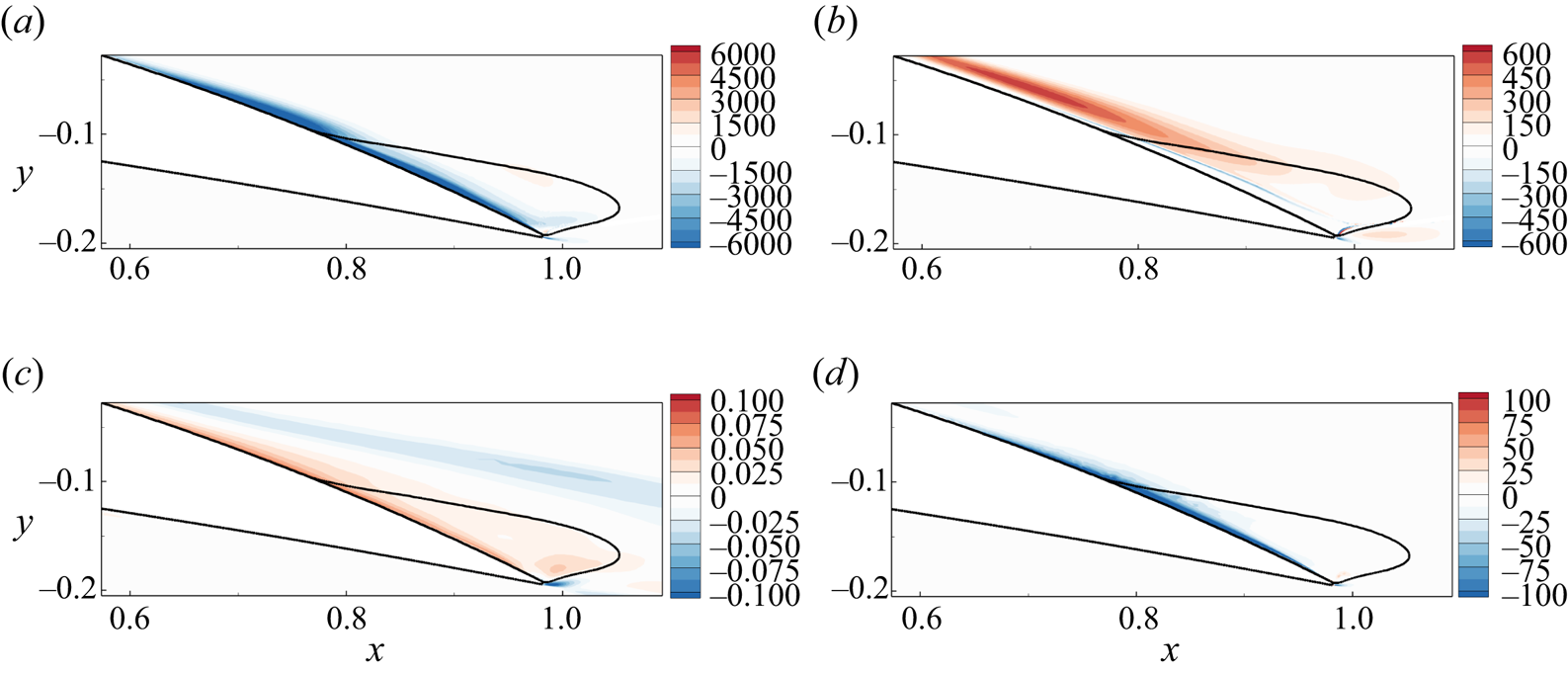
Wall-normal profiles at  $x_{c,u}=0.75$ of various quantities in figure 20 (solid curves): (a) streamwise mean-velocity error
 $|\delta \bar {u} | = | \bar {u}_{d} - \bar {u}|$, (b) streamwise component of the sensitivity function
 $|\boldsymbol {\nabla }_{{\bar {u}}} \lambda |$ and (c) local contribution to the eigenvalue variation
 $|\boldsymbol {\nabla }_{\boldsymbol {\bar {u}}} \lambda \boldsymbol {\cdot } \delta \boldsymbol {\bar {u}}|$. The dashed curve in (a) shows the profile of
 $1-\rho _{RS}$, where
 $\rho _{RS}$ is the correlation between the anisotropic Reynolds stress and mean strain rate tensors as evaluated from DNS (see (4.3)).

The residual difference between the DNS and assimilated mean-flow velocities  $\delta \boldsymbol {\bar {u}}=\boldsymbol {\bar {u}}_{d} - \boldsymbol {\bar {u}}$, which has been minimized during the data-assimilation procedure, is displayed in figure 20(c) for the streamwise component. As evoked in § 4.1, this error is small but non-negligible. The largest values are obtained near the airfoil's wall (red region) as well as in the upper part of the shear layer (blue region). Examining more carefully the velocity error in the attached turbulent boundary layer as displayed in figure 21(a) at station
 $x_{c,u}=0.75$, we identify two regions of significant residual velocity error (solid curve). The dominant one is very close to the walls (
 $d/\delta \leqslant 0.05$) while the subdominant one is near the edge of the boundary layer (
 $d/\delta \geqslant 0.85$).
Using the sensitivity function  $\boldsymbol {\nabla }_{\boldsymbol {\bar {u}}} \lambda$, we can now estimate the uncertainty/variation in the eigenvalue that is induced by such residual mean-flow velocity error according to (2.21). The scalar field
 $\boldsymbol {\nabla }_{\boldsymbol {\bar {u}}} \lambda \boldsymbol {\cdot } ( \boldsymbol {\bar {u}}_{d} - \boldsymbol {\bar {u}} )$ quantifies the uncertainty in the eigenvalue that is induced by the local mean-flow velocity error. It is displayed in figure 20(d). The spatial integration of this field yields the global uncertainty in the eigenvalue, which is around
 $\delta \lambda \approx -0.1$ for the present mode A. This eigenvalue variation is non-negligible in comparison with the maximum growth rate of mode A which is shown in figure 15(a). We would thus obtain that mode A is stable for the angle
 $\alpha =11^{\circ }$, which is not in disagreement with the experimental observation since stall cells are observed for
 $\alpha \geqslant 12^{\circ }$. However, it may be worth keeping in mind that, in addition to being restricted to a linearity assumption, the present uncertainty quantification does not take into account the impact of residual errors in the assimilated turbulent eddy viscosity, the latter being difficult to accurately evaluate by lack of a reliable reference eddy viscosity, so that the present value of
 $\delta \lambda$ should be considered as only an estimate.
Coming back to figure 20(d) and comparing it with 20(c), it is interesting to note that the residual mean-velocity errors close to the airfoil's wall and near the separation point are mainly responsible for the eigenvalue uncertainty. The residual errors in the shear layer are thus of minor importance for predicting the growth rate of mode A. Examining more carefully the contribution to  $\delta \lambda$ in the attached turbulent boundary layer (figure 21c), we see that only the mean-flow velocity errors in the viscous sublayer induce uncertainties in the eigenvalue. These residual mean-velocity errors and subsequent eigenvalue uncertainty can be attributed to the Boussinesq hypothesis on which is based the present turbulent model, as illustrated in the following. In this hypothesis, the anisotropic part of the Reynolds stress tensor is assumed to be linearly proportional to the strain rate tensor, as stated by (2.4). The validity of that hypothesis can be here quantified through the DNS results (still at
 $\alpha =11^{\circ }$), from which are extracted a time- and spanwise-averaged reference anisotropic Reynolds stress tensor
 $\boldsymbol {\bar {R}}^{a}_{d}$ and strain rate tensor
 $\boldsymbol {S}(\boldsymbol {\bar {u}}_{d})$. The correlation, or alignment
 $\rho _{RS}$ between these two tensors may be evaluated according to
 \begin{equation} \rho_{RS} = \frac{|
\boldsymbol{\bar{R}}^{a}_{d} :
\boldsymbol{S}(\boldsymbol{\bar{u}}_{d}) |}{ ||
\boldsymbol{\bar{R}}^{a}_{d} ||
||\boldsymbol{S}(\boldsymbol{\bar{u}}_{d}) ||},
\end{equation}
where  $|| \boldsymbol {\cdot } ||$ here denotes the tensor norm defined as
 $|| \boldsymbol {\cdot } ||^2 = \boldsymbol {\cdot } : \boldsymbol {\cdot }$, while
 $:$ denotes the tensor contraction. For
 $\rho _{RS}=1$ (
 $\rho _{RS}=0$), the tensors are fully aligned (orthogonal) and therefore the hypothesis is valid (invalid). The dashed curve in figure 21(a) displays the quantity
 $1-\rho _{RS}$ in the attached turbulent boundary layer at station
 $x_{c,u}=0.75$. Near the outer edge of the boundary layer, that quantity is close to 0 and the Boussinesq hypothesis is then valid in that region. On the other hand, it gets very close to 1 when approaching the airfoil's wall, which coincides with the region where the residual mean-velocity errors are maximum (solid curve). This demonstrates that the Boussinesq hypothesis is not valid in the viscous sublayer of that turbulent boundary layer, thus explaining the inability of the data-assimilation algorithm to further reduce the mean-velocity error in that region. The accuracy in the prediction of the stall cells using the present combination of data assimilation and linear stability analysis is therefore limited here by the choice of a linear eddy-viscosity turbulence model. The use of nonlinear eddy-viscosity models, as in Kitsios et al. (Reference Kitsios, Cordier, Bonnet, Ooi and Soria2010), based on the expansion of the Reynolds stress tensor proposed by Pope (Reference Pope1975), is a recommended approach for improving the present results in future studies.
4.4. Influence of the correction on the stability analyses of the assimilated mean flows
Since the correction  $\bar {f}_{1}=\bar {\nu } \bar {g}_{1}$ leads to the best estimation of the mean-flow velocity field, as recalled in the first row of table 4, the stability of the latter has been preferentially investigated so far. We now investigate the stability of the assimilated mean flows that have been obtained with the other corrections,
 $\bar {f}_{0}= \bar {g}_{0}$ and
 $\bar {f}_{2}=\bar {\nu }^2 \bar {g}_{2}$, so as to investigate the influence of the choice of the correction on the results of stability analysis. Figure 22 shows the growth rate of the leading eigenvalue as a function of the wavenumber, computed with the perturbed eddy-viscosity approach and the assimilated mean-flow velocities obtained with the corrections
 $\bar {f}_0$ (dash-dotted curve),
 $\bar {f}_1$ (solid curve) and
 $\bar {f}_2$ (dashed curve). First of all, we clearly observe a variation in the growth rate that is of similar order of magnitude to that when comparing frozen and perturbed eddy-viscosity approaches around the assimilated flow for the correction
 $\bar {f}_1$ (see figure 17a). Results obtained with the two multiplicative corrections (solid and dashed curves) are very similar for
 $\beta \leqslant 5$. For larger values, the growth rate obtained with the correction
 $\bar {f}_{2}$ is systematically larger and is unstable in the range
 $5 \leqslant \beta \leqslant 20$. Recalling that the stall cells are observed in the experiments for
 $\beta \sim 4$, we can conclude that results obtained with the correction
 $\bar {f}_{2}$ lack selectivity in the transverse wavenumber. Interestingly, the stability analysis of the mean flow corrected with
 $\bar {f}_{0}$ (dash-dotted curve) better selects the wavenumber since the maximal value of the growth rate is obtained for
 $\beta \sim 5$ and the growth rate for larger wavenumbers is strongly damped. Therefore, the selectivity in the wavenumber is better with the correction
 $\bar {f}_0$. Examining now the value of this growth rate, it is significantly lower for the correction
 $\bar {f}_{0}$ than for
 $\bar {f}_{1}$. It is difficult to determine which correction gives the best estimation, since there is no reference value for the growth rate. Recalling that no stall cells are observed for angle of attack
 $\alpha =11^{\circ }$, the stable or marginally stable eigenvalues obtained with the two corrections are both possible.
Growth rate of the leading eigenvalue  $\sigma _L$ as a function of the wavenumber
 $\beta$ (computed with the perturbed eddy-viscosity approach) for assimilated mean flows at
 $\alpha =11^{\circ }$ obtained with the correction
 $\bar {f}_{0}$ (dash-dotted curve),
 $\bar {f}_{1}$ (solid curve) and
 $\bar {f}_{2}$ (dashed curve).

Influence of the choice of the correction  $\bar {f}_{n}$ (
 $n=0,1,2$) on the stability of the assimilated mean flows (in the perturbed eddy-viscosity approach). The first row recalls the decrease in the discrepancies between the assimilated flows obtained with the different corrections and the reference DNS mean-flow velocity compared with baseline RANS. The second and third rows show the growth rate of the eigenvalue computed at
 $\beta =5$ and its variation
 $\Delta \sigma = \sigma (\bar {f}_n)-\sigma (\bar {f}_1)$. The fourth and fifth rows show the
 $L_2$ norm of the mean-flow velocity variation
 $\Delta \boldsymbol {\bar {u}}(\bar {f}_n)=\boldsymbol {\bar {u}}(\bar {f}_{n})-\boldsymbol {\bar {u}}(\bar {f}_{1})$ and the corresponding variation of the growth rate
 $(\delta \sigma )_{\boldsymbol {\bar {u}}}$ computed with (4.4).
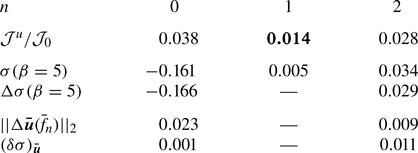
The variations in the growth rate between the different cases seen in figure 22 are due either to variations in the assimilated mean-flow velocity  $\boldsymbol {\bar {u}}(\bar {f}_{n})$, to variations in the assimilated eddy-viscosity variable
 $\bar {\nu }(\bar {f}_{n})$ or to the structural perturbation of the eigenvalue problem. For multiplicative corrections (i.e.
 $n>0$), the term
 $\bar {h}_{n} = n \bar {\nu }^{n-1} \bar {g}_{n}$ indeed appears in the Jacobian operator (2.18) so that the correction
 $\bar {g}_{n}$ directly impacts the stability analysis. In this regard, the correction
 $\bar {f}_{0}$ should possibly be preferred over multiplicative corrections to avoid that additional complexity. As a first step to disentangle the above-mentioned various factors to variations in the stability results, we estimate, based on a sensitivity analysis, the growth rate variation for the leading mode at
 $\beta =5$ that is specifically induced by velocity variations between the assimilated mean flows. This analysis is similar to that developed in § 4.3. Since the error between the assimilated and reference DNS mean-flow velocities is minimal for the correction
 $\bar {f}_{1}$, we use the corresponding mean-flow velocity
 $\boldsymbol {\bar {u}}(\bar {f}_{1})$ as reference in this subsection. The difference in mean-flow velocities is thus here defined as
 $\Delta \boldsymbol {\bar {u}}(\bar {f}_{n})= \boldsymbol {\bar {u}}(\bar {f}_{n})-\boldsymbol {\bar {u}}(\bar {f}_{1})$ where
 $n=0$ or
 $n=2$. In table 4, we report the
 $L_2$ norm of this difference, defined as
 $|| \Delta \boldsymbol {\bar {u}}(\bar {f}_{n}) ||_2 = ( \int _\varOmega \Delta \boldsymbol {\bar {u}} \boldsymbol {\cdot }\Delta \boldsymbol {\bar {u}} \,\textrm {d}\varOmega )^{1/2}$. This global measure of the velocity variation is very small for the correction
 $\bar {f}_{2}$ and around three times larger for
 $\bar {f}_{0}$. However, it appears that these velocity variations do not fully explain the variations in the growth rate
 $\Delta \sigma$ seen in figure 22 (black circles) and also reported in table 4 (third row). Indeed, the variation in the eigenvalue induced by these velocity variations may be evaluated as
 \begin{equation} (\delta \lambda)_{\boldsymbol{\bar{u}}} = \int_{\varOmega} \boldsymbol{\nabla}_{\boldsymbol{\bar{u}}} \lambda \boldsymbol{\cdot}\Delta \boldsymbol{\bar{u}}(\bar{f}_{n}), \end{equation}
i.e. the integral over space of the local product between the velocity variation and  $\boldsymbol {\nabla }_{\boldsymbol {\bar {u}}} \lambda$, the sensitivity of the eigenvalue to mean-flow variation, computed here for the assimilated mean flow with the correction
 $\bar {f}_{1}$ as already performed in § 4.3. Figure 23(a,c) displays the spatial distribution of the velocity difference, defined as
 $|\Delta \boldsymbol {\bar {u}}(\bar {f}_{n})| = ( \Delta \boldsymbol {\bar {u}}\boldsymbol {\cdot }\Delta \boldsymbol {\bar {u}} )^{1/2}$, for the corrections
 $n=0$ and
 $n=2$. Figure 23(b,d) reports the local contribution to the eigenvalue variation, i.e.
 $\boldsymbol {\nabla }_{\boldsymbol {\bar {u}}} \lambda \boldsymbol {\cdot }\Delta \boldsymbol {\bar {u}}(\bar {f}_{n})$, for
 $n=0$ and
 $n=2$. Starting with the correction
 $\bar {f}_{2}$, the difference of the assimilated mean flow from that obtained for
 $\bar {f}_{1}$ is non-negligible in the attached boundary layer, inside the recirculation region and close to the trailing edge, as seen in figure 23(c). Due to the spatial distribution of the eigenvalue sensitivity displayed in figure 20, the velocity differences close to the separation point and inside the recirculation region induce non-negligible positive variation of the eigenvalue, as seen in figure 23(d). After integration over space, we obtain that
 $(\delta \sigma )_{\boldsymbol {\bar {u}}}=0.011$, showing that the actual eigenvalue variation
 $\Delta \sigma = 0.029$ observed in figure 22 for
 $\beta =5$ (black circles) can be only partially explained by the velocity differences between the corrections. Examining now results for the correction
 $\bar {f}_{0}$, the difference of the assimilated mean flow from that obtained for
 $\bar {f}_{1}$ is very small in the attached boundary layer and inside the recirculation region close to the separation point, while a much larger difference is observed close to the trailing edge (see figure 23a). This larger velocity difference does not induce any variation of the eigenvalue, as seen in figure 23(b), except very close to the trailing edge. The variation of the eigenvalue induced by the velocity variation is eventually very small (
 $\delta \sigma )_{\bar {u}}=0.001$ and cannot explain the large variation of the eigenvalue
 $\Delta \sigma = -0.166$ observed in figure 22. In that case, the impact of velocity differences on the eigenvalue variation seems secondary compared with differences in the eddy-viscosity field or in the structure of the Jacobian matrix.
Influence of the assimilated mean-flow velocity  $\boldsymbol {\bar {u}}(\bar {f}_{n})$ on the stability analysis. (a,c) Norm of the difference between the assimilated velocity fields
 $\Delta \boldsymbol {\bar {u}}(\bar {f}_{n})=\boldsymbol {\bar {u}}(\bar {f}_{n})-\boldsymbol {\bar {u}}(\bar {f}_{1})$ and (b,d) local contribution to the growth rate of the eigenvalue induced by such differences determined with (4.4) for (a,b)
 $n=0$ and (c,d)
 $n=2$.

These results clearly indicate that a small difference in the mean-flow velocities, which is the objective of the data-assimilation algorithm proposed here, is not always sufficient to guarantee the convergence of the leading eigenvalue, because the impact of the correction or of the assimilated mean eddy-viscosity on results of the stability analysis is not negligible. In future studies, the mean-flow estimation with data assimilation and its stability analysis should be more intertwined, so as to provide a better estimation of the leading eigenvalues. The eigenvalue sensitivity field to mean-flow velocity variations could be used as a weight function in the definition  $\mathcal {J}^{u}$ of the cost function (2.13) so as to minimize the velocity difference preferentially in mean-flow regions of interest for the stability analysis. To further investigate the impact of the correction on the eigenvalue, it might also be interesting to determine the sensitivity of the eigenvalue to the correction
 $\bar {g}_{n}$ so as to determine sensitive mean-flow regions. Such information could then be used to weight the penalization term
 $\mathcal {J}^{g_n}$ in the cost function so as to reduce the impact of the correction on the eigenvalue. We should also remark that the effective correction is partially linearized in the present study. Indeed, the correction
 $\bar {g}_{n}$ is somehow frozen as it is independent of the mean-flow state. The neural-network-augmented turbulence model as proposed by Singh & Duraisamy (Reference Singh and Duraisamy2016) would be interesting to obtain a correction that depends on input features depending on the flow state. A proper linearization of the correction term in the turbulence model could thus be achieved and would probably change results of the eigenvalue analysis for the present flow configuration. Finally, the influence of the turbulence model on the present results should be addressed in future studies.
5. Conclusion
In this paper we investigated the formation of three-dimensional cellular structures, known as stall cells, on the suction side of a NACA4412 airfoil at Reynolds number  $Re=350\,000$ for angles of attack in the range
 $10^{\circ } \leqslant \alpha \leqslant 12^{\circ }$. In the framework of a triple decomposition of the flow, the turbulent flow may be described with the RANS equations with a linear eddy-viscosity assumption for modelling the Reynolds stress tensor. The turbulent eddy viscosity is here described with the Spalart–Allmaras model, resulting in closed form of the equations governing the turbulent flow.
First, we showed that the baseline RANS model fails to determine the critical angle of attack for the onset of stall cells. The two-dimensional mean-flow velocity field does not capture the trailing-edge flow separation that occurs in the DNS performed by Gleize et al. (Reference Gleize, Costes and Mary2022) for angles in pre-stall conditions. A global stability analysis of the two-dimensional turbulent mean flow then predicts the destabilization of a three-dimensional stall cell mode, in agreement with previous results by Plante et al. (Reference Plante, Dandois, Beneddine, Laurendeau and Sipp2021). However, the critical angle of attack is largely superior to that observed in the experiments performed for the same airfoil, angles of attack and Reynolds number in a subsonic wind tunnel at ONERA, Chalais Meudon. This disagreement is preferentially attributed to the inability of the RANS simulations in correctly capturing the trailing-edge mean-flow separation.
In order to improve the predictive capability of a global stability analysis around a turbulent mean flow estimated with RANS equations, we proposed an adjoint-based data-assimilation method that aims at determining corrective fields in the model equation so as to minimize the discrepancies between the RANS-estimated and DNS-reference mean-flow velocities. Several types of correction fields defined as source terms in the turbulence model have been shown to strongly improve the estimation of the full mean-flow velocity while giving a consistent eddy-viscosity field and model. For the flow configuration investigated here, a multiplicative source term is the correction field yielding the best estimation of the two-dimensional mean flow. To predict the onset of stall cells, two approaches of the linear stability analysis around this best estimation of the mean flow were then considered and compared. In the perturbed eddy-viscosity approach, perturbations of the velocity, pressure and turbulence model's variables are considered. The latter are neglected in the frozen eddy-viscosity approach that is most commonly used for the linear analyses of turbulent wall-bounded and jet flows. The two approaches could be investigated in this framework of data-consistent RANS model, since the turbulence model has been linearized in addition to the RANS equations. Both approaches could identify stationary low-wavenumber and high-wavenumber modes, which were referred to as modes A and B, respectively, whose structures correspond to streaks of streamwise velocity and strong transverse velocities. Through comparisons with the experimental results, we have shown that the perturbed eddy-viscosity approach yields a significantly better prediction of the onset of stall cells compared with the other investigated approaches as (i) it predicts the critical angle of attack more precisely and (ii) it is much more accurate and selective in terms of the unstable transverse wavelengths. Concerning this latter aspect, it was indeed shown that the frozen eddy-viscosity approach predicts that B modes become first unstable, while the corresponding wavelengths are far smaller than the experimental observations. This was observed no matter if the frozen approach was performed around assimilated mean flows or DNS ones with consistent eddy-viscosity fields in the sense of Pickering et al. (Reference Pickering, Rigas, Schmidt, Sipp and Colonius2021).
The aforementioned results therefore demonstrate (i) the benefits of relying on data assimilation to get accurate mean-flow descriptions that are solutions of a calibrated turbulence model and (ii) the need to not only include an eddy-viscosity field but to also account for its linear perturbations using this calibrated model in stability analyses for the prediction of stall cells. More generally, the present methodology appears as a promising approach for the accurate and yet computationally tractable estimation of coherent flow phenomena in turbulent configurations.
Several aspects of the method that deserve further investigations have been briefly addressed. Firstly, the influence of the residual error in the velocity of the assimilated mean flow was investigated using sensitivity analysis of the stall cell modes. The corresponding eigenvalue was shown to be sensitive in flow regions where the Boussinesq hypothesis is not valid and the residual velocity errors thus remain non-negligible. Such results clearly indicate that a more sophisticated turbulent flow model might be considered in future studies. In future studies, information on the eigenvalue sensitivity might also be included in the data-assimilation method used to obtain the mean flow so as to favour the convergence of the stability analysis results and better constrain the chosen model correction. Secondly, we have shown that the different correction fields used in the mean-flow equations have a non-negligible influence on the results of stability analysis. The selection in the transverse wavelength of the stall cell mode was notably different. Interestingly, we have shown that differences in the growth rate are not necessarily due to differences in the mean-flow velocity but also to the correction itself. To better investigate the influence of the correction that has been frozen in the present study, we recommend obtaining a data-consistent turbulent model using the paradigm of machine learning field inversion proposed by Singh & Duraisamy (Reference Singh and Duraisamy2016). By linearizing also the correction field, we may better assess its influence on the stability results and hopefully reduce it. Additionally, such neural network turbulence models have promising extrapolation capability that could be used for cases where no reference data are available, facilitating parametric studies and the identification of critical stability conditions. Finally, we should say that the data-consistent RANS model approach presented here is not limited to the use of full mean-flow velocity data, as done in the present study. As a perspective to the present work, we could use sparse data, such as wall pressure or wall skin-friction measurements around the airfoil, to better estimate the mean flow and its stability. By doing so, we could extend the method to more complex flow configurations for which generating full mean-flow velocity with high-fidelity simulations is still not feasible nowadays.
Acknowledgements
The authors are grateful to M. Costes, V. Gleize, I. Mary and F. Richez for the generation and processing of the DNS results. The authors also thank F. Bouvier and V. Brion for producing the experimental data.
Funding
This project received funding from the European Union's Horizon 2020 research and innovation programme under Marie Sklodowska-Curie grant agreement no. 955923.
Declaration of interests
The authors report no conflict of interest.
Appendix A. Spalart–Allmaras turbulent model
The Spalart–Allmaras turbulence model introduced in § 2.1 corresponds to a transport equation for a turbulent viscosity variable denoted  $\left \langle \tilde {\nu }\right \rangle$. The eddy-viscosity variable
 $\left \langle \nu _{t}\right \rangle$ depends on that turbulent viscosity variable according to
 \begin{equation} \left\langle \nu_{t}\right\rangle (\left\langle \tilde{\nu}\right\rangle ) = \left\langle \tilde{\nu}\right\rangle f_{v1} ( \chi ) , \quad f_{v1} = \frac{\chi^3}{\chi^3 + c_{v1}^3} , \end{equation}
where  $\chi = \left \langle \tilde {\nu }\right \rangle Re$ and
 $c_{v1}=7.1$. The equation governing
 $\left \langle \tilde {\nu }\right \rangle$ is
 \begin{equation} \partial_{t} \left\langle \tilde{\nu} \right\rangle + T(\left\langle \boldsymbol{u} \right\rangle ,\left\langle \tilde{\nu} \right\rangle ) = 0 , \end{equation}
where the nonlinear operator  $T$ is defined as
 \begin{equation} T(\left\langle \boldsymbol{u} \right\rangle ,\left\langle \tilde{\nu} \right\rangle ) = (\left\langle \boldsymbol{u}\right\rangle \boldsymbol{\cdot} \boldsymbol{\nabla}) \left\langle \tilde{\nu} \right\rangle -\boldsymbol{\nabla} \boldsymbol{\cdot} (\eta(\left\langle \tilde{\nu} \right\rangle ) \boldsymbol{\nabla} \left\langle \tilde{\nu} \right\rangle ) - s(\left\langle \tilde{\nu}\right\rangle ,\boldsymbol{\nabla} \left\langle \tilde{\nu}\right\rangle ,\boldsymbol{\nabla} \left\langle \boldsymbol{u}\right\rangle ). \end{equation}
The first two terms correspond to convection and diffusion, respectively. In the latter, the effective viscosity is  $\eta (\left \langle \tilde {\nu }\right \rangle ) = \sigma ^{-1} (1/Re + \left \langle \tilde {\nu }\right \rangle )$, where
 $\sigma =2/3$. The third term in (A3) is a nonlinear source term
 $s$ defined as the sum of cross-diffusion
 $\mathcal {C}$, production
 $\mathcal {P}$ and destruction
 $\mathcal {D}$ terms, according to
 \begin{equation} s = (1 - f_{t2}) \boldsymbol{\cdot} \underbrace{c_{b1} \tilde{S} \left\langle \tilde{\nu}\right\rangle }_{\mathcal{P}} +\underbrace{\sigma^{{-}1} c_{b2} \lvert \boldsymbol{\nabla} \left\langle \tilde{\nu}\right\rangle \lvert^2}_{\mathcal{C}} - \underbrace{c_{w1} f_{w} \frac{\left\langle \tilde{\nu}\right\rangle }{d^2} }_{\mathcal{D}}, \end{equation}
where the exact definition of each term can be found in Spalart & Allmaras (Reference Spalart and Allmaras1992). The term  $f_{t2}$ which multiplies the turbulence production term is known as the tripping term. This scalar field allows one to trigger transition to turbulence, in particular at the locations defined in § 3.2. When
 $f_{t2}=1$, the production term is set to zero and the boundary layer stays laminar while when we transition to
 $f_{t2}=0$ at the prescribed locations on the upper and lower surface, we initiate the production of turbulence.
Appendix B. Definitions of operators used in RANS and turbulence model equations
The two-dimensional turbulent base flow satisfies the governing equation (2.11a–d) where the residual vectors for the RANS and turbulent model equations are defined as
 \begin{equation} \left.\begin{gathered}\boldsymbol{R}_{\boldsymbol{u}}^{0}(\boldsymbol{\bar{u}},\bar{P},\bar{\nu}_t(\bar{\nu})) =\boldsymbol{\nabla}_{0} \boldsymbol{\cdot} \left( \boldsymbol{\bar{u}} \otimes \boldsymbol{\bar{u}} \right) + \boldsymbol{\nabla}_{0} \bar{P} - \boldsymbol{\nabla}_{0} \boldsymbol{\cdot} \left[ 2 \left( \frac{1}{Re} + \overline{\nu_t}(\bar{\nu}) \right) \boldsymbol{S}_{0}(\boldsymbol{\bar{u}}) \right], \\ T^{0}(\boldsymbol{\bar{u}},\bar{\nu}) = (\boldsymbol{\bar{u}}\boldsymbol{\cdot} \boldsymbol{\nabla}_{0}) \bar{\nu} - \boldsymbol{\nabla}_0 \boldsymbol{\cdot} (\eta(\bar{\nu}) \boldsymbol{\nabla}_0 \bar{\nu}) - s(\bar{\nu},\boldsymbol{\nabla}_{0} \bar{\nu}, \boldsymbol{\nabla}_{0} \boldsymbol{\bar{u}}), \end{gathered}\right\} \end{equation}
where the spatial operator  $\boldsymbol {\nabla }_{0}=(\partial _{x},\partial _{y},0)^{\textrm {T}}$ denotes the two-dimensional gradient and
 $\boldsymbol {S}_{0}(\boldsymbol {\bar {u}})=1/2 ( \boldsymbol {\nabla }_{0} \boldsymbol {\bar {u}} + \boldsymbol {\nabla }_{0} \boldsymbol {\bar {u}}^{T} )$.
In the perturbed eddy-viscosity approach, the three-dimensional perturbations are investigated by computing the leading eigenvalues/eigenmodes of the eigenproblem (2.18) where the blocks in the Jacobian operator are defined as
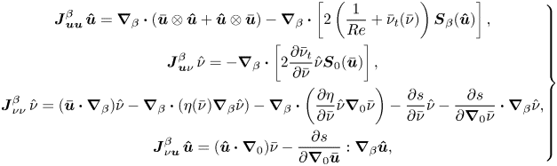 \begin{align} \left.\begin{gathered} \boldsymbol{J}_{\boldsymbol{u} \boldsymbol{u}}^{\beta} \, \boldsymbol{\hat{u}} = \boldsymbol{\nabla}_{\beta} \boldsymbol{\cdot} \left( \boldsymbol{\bar{u}} \otimes \boldsymbol{\hat{u}} + \boldsymbol{\hat{u}} \otimes \boldsymbol{\bar{u}} \right) - \boldsymbol{\nabla}_{\beta} \boldsymbol{\cdot} \left[ 2 \left( \frac{1}{Re} + \bar{\nu}_t(\bar{\nu}) \right) \boldsymbol{S}_{\beta}( \boldsymbol{\hat{u}}) \right], \\ \boldsymbol{J}_{\boldsymbol{u} \nu}^{\beta} \, \hat{\nu} ={-} \boldsymbol{\nabla}_{\beta} \boldsymbol{\cdot} \left[ 2 \frac{\partial \bar{\nu}_t }{\partial \bar{\nu}} \hat{\nu}\boldsymbol{S}_{0}( \boldsymbol{\bar{u}}) \right], \\ \boldsymbol{J}_{\nu \nu}^{\beta} \, \hat{\nu} = (\boldsymbol{\bar{u}}\boldsymbol{\cdot} \boldsymbol{\nabla}_{\beta}) \hat{\nu} - \boldsymbol{\nabla}_{\beta} \boldsymbol{\cdot} (\eta(\bar{\nu})\boldsymbol{\nabla}_\beta \hat{\nu}) -\boldsymbol{\nabla}_{\beta} \boldsymbol{\cdot} \left(\frac{\partial\eta}{\partial \bar{\nu}}\hat{\nu}\boldsymbol{\nabla}_0 \bar{\nu}\right) - \frac{\partial s}{\partial \bar{\nu}} \hat{\nu} - \frac{\partial s}{\partial \boldsymbol{\nabla}_{0} \bar{\nu}} \boldsymbol{\cdot} \boldsymbol{\nabla}_{\beta}\hat{\nu}, \\ \boldsymbol{J}_{\nu \boldsymbol{u} }^{\beta} \, \boldsymbol{\hat{u}} = (\boldsymbol{\hat{u}}\boldsymbol{\cdot} \boldsymbol{\nabla}_{0}) \bar{\nu} - \frac{\partial s}{\partial \boldsymbol{\nabla}_{0} \boldsymbol{\bar{u}}} : \boldsymbol{\nabla}_{\beta}\boldsymbol{\hat{u}} , \end{gathered}\right\} \end{align}
where  $\boldsymbol {\nabla }_\beta = (\partial _x, \partial _y, \textrm {i}\beta )$ is the gradient operator in three dimensions and
 $\boldsymbol {S}_{\beta }(\boldsymbol {\hat {u}})=1/2 ( \boldsymbol {\nabla }_{\beta } \boldsymbol {\hat {u}} + (\boldsymbol {\nabla }_{\beta } \boldsymbol {\hat {u}})^{\textrm {T}})$, where
 $\boldsymbol {\hat {u}}=(\hat {u},\hat {v},\hat {w})^{\textrm {T}}$. Note that the two-dimensional operators that are involved
 $\boldsymbol {J}_{\boldsymbol {u} \boldsymbol {u}}^{0}$,
 $\boldsymbol {J}_{\boldsymbol {u} \nu }^{0}$,
 $\boldsymbol {J}_{\nu \nu }^{0}$ and
 $\boldsymbol {J}_{\nu \boldsymbol {u} }^{0}$ involved when solving the two-dimensional mean-flow equations (2.11a–d) (through a quasi-Newton method; see § 2.6) and the adjoint problem (2.15) are obtained from the above definition by considering
 $\beta =0$.
Appendix C. Effect of the penalization parameter on the assimilated Reynolds stress tensor
As detailed in § 2.3, the cost function  $\mathcal {J}$ in (2.13) involves the parameter
 $m$ which weights a penalty term that prevents from overfitting. The optimal value for this parameter is determined in § 4.1.1 for the correction
 $\bar {f}_1$ through an L-curve analysis, as illustrated in figure 7(b). In this appendix, it is shown that the thus-obtained value for
 $m$ is also almost optimal to model the Reynolds stress tensor. Figure 24(a) reports the following metric that quantifies the discrepancies between the anisotropic part of the mean Reynolds stress tensor as evaluated by DNS
 $\boldsymbol {\bar {R}}^{a}_{d}$ or for assimilated mean flows
 $\boldsymbol {\bar {R}}^{a}$ (according to (2.4)) at
 $\alpha =11^{\circ }$ for different values of the penalization parameter:
 \begin{equation} E^{RST}=\int_{\varOmega_m} \Delta \boldsymbol{\bar{R}}^{a} : \Delta \boldsymbol{\bar{R}}^{a} \, {\rm d}\varOmega_m , \quad \Delta \boldsymbol{\bar{R}}^{a}=\boldsymbol{\bar{R}}^{a} - \boldsymbol{\bar{R}}^{a}_{d}. \end{equation}
It appears that the value of  $E^{RST}$ is close to be minimum for
 $m=10^{-4}$ (filled circle), i.e. the value that was identified through the L-curve analysis. Significantly increasing or decreasing
 $m$ would thus induce a deterioration in the modelled Reynolds stress tensor. The improvement with respect to baseline RANS results is appreciable and is illustrated through figures 24(b)–24(d), which report the Reynolds stress
 $\overline {u''v''}$ as obtained from DNS results, from baseline RANS results and for the assimilated mean flow that corresponds to
 $m=10^{-4}$, respectively. The baseline RANS results significantly underestimate the magnitude of
 $\overline {u''v''}$ near the trailing edge and in the recirculation region, which is satisfactorily corrected through the data-assimilation procedure.
(a) Error on the Reynolds stress tensor  $E^{RST}$ (see (C1a,b)) normalized by its value for baseline RANS
 $E^{RST}_0$ for the assimilated flows at
 $\alpha =11^{\circ }$ that are obtained with different values of the penalization coefficient
 $m$ (see (2.13)). Reynolds stress
 $\overline {u''v''}$ as estimated (b) by DNS, (c) by baseline RANS and (d) for the assimilated flow with
 $m=10^{-4}$ (filled circle in a).

Appendix D. Determination of eddy viscosity consistent with the reference mean flow from DNS
To perform resolvent analyses of turbulent mean flows in isothermal jets, Pickering et al. (Reference Pickering, Rigas, Schmidt, Sipp and Colonius2021) proposed to determine an eddy-viscosity field, denoted  $\bar {\nu }_{t}^{c}$, that is consistent with the reference mean flow by minimizing the residual of the momentum equations. In order to consider a well-posed problem, this is here formulated by minimizing the following cost function:
 \begin{equation} \mathcal{G} (\bar{\nu}_{t}^{c}) = \int_{\varOmega_{m}} \left\|\boldsymbol{R}^{0}_{\boldsymbol{u}}(\boldsymbol{\bar{u}}_d,\bar{P}_d,\bar{\nu}_t^{c}) \right\|^{2} \,{\rm d}\varOmega_{m}, \end{equation}
where  $\boldsymbol {R}^{0}_{\boldsymbol {u}}(\boldsymbol {\bar {u}}_d,\bar {P}_d,\bar {\nu }_t^{c})$ refers to the residual of the RANS momentum equations in (B1). Assuming that both
 $\boldsymbol {\bar {u}}_d$ and
 $\bar {P}_d$ are known through DNS, the minimizing consistent eddy viscosity is obtained through inverting the following linear system:
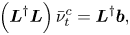 \begin{equation} \left(\boldsymbol{L}^{{{\dagger}}} \boldsymbol{L} \right) \bar{\nu}_t^{c} = \boldsymbol{L}^{{{\dagger}}} \boldsymbol{b}, \end{equation}
where
 \begin{equation} \left.\begin{gathered}
\boldsymbol{L} \left(\star \right) =
\boldsymbol{\nabla}_{0} \boldsymbol{\cdot} \left[ 2
\left(\star\right)
\boldsymbol{S}_{0}(\boldsymbol{\bar{u}}_{d})\right],\\
\boldsymbol{b} = \boldsymbol{\nabla}_{0} \boldsymbol{\cdot}
\left( \boldsymbol{\bar{u}}_{d} \otimes
\boldsymbol{\bar{u}}_{d} \right) + \boldsymbol{\nabla}_{0}
\bar{P}_{d} - \boldsymbol{\nabla}_{0} \boldsymbol{\cdot}
\left[ \frac{2}{Re}
\boldsymbol{S}_{0}(\boldsymbol{\bar{u}}_{d}) \right],
\end{gathered}\right\}
\end{equation}
and where  $\boldsymbol {L}^{{\dagger} }$ refers to the adjoint of the operator
 $\boldsymbol {L}$.


 Open access

