1. Introduction

The “likelihoodist,” or “evidentialist,” school of thought in statistics is well known among philosophers, more so perhaps than among scientists or even statisticians, in large part due to Hacking (Reference Hacking1965). One way to distinguish evidentialism from the other major schools—frequentism and Bayesianism—is to note that evidentialism alone focuses on the assessment of statistical evidence as its principal task, rather than decision making or the rank-ordering of beliefs.Footnote ¹

It might be thought, therefore, that evidentialism would be the predominant approach to statistical inference in science, where quantifying evidence is usually the main objective. (If you do not agree, try getting scientists to stop using the p-value as a measure of the strength of the evidence.) But frequentism, and to a lesser extent Bayesianism, predominate in the scientific literature, while evidentialism is virtually unseen. Why is this? I argue here that the fault lies with evidentialism’s failure thus far to address the problem of calibrating the units in which evidence is to be measured. Since meaningful calibration is the sine qua non of scientific measurement, this turns out to be the loose thread that causes the cloth to unravel when we pull on it.

Before proceeding, it may be worth noting some things I will and will not be talking about. First, I am concerned only with statistical evidence and will not be considering the concept of evidence as it appears in other contexts (e.g., in legal proceedings). Second, I will treat statistical evidence as a relationship between data and hypotheses under a model that can be expressed in the form of a likelihood (as defined below). On this view, data do not possess inherent evidential meaning on their own but only take on evidential meaning in the context of their relationships to particular hypotheses, with the nature of those relationships governed by the form of the likelihood. I will not be concerned here with measurement problems associated with the data themselves.Footnote ² Third, I am interested here solely in addressing the question of whether this relationship between data and hypotheses can be rigorously quantified. If the answer is yes, then presumably the degree of evidence could play a role in decision making (deciding how strong is strong enough when it comes to evidence) or in guiding belief, but I will not be addressing these topics here. It is one hallmark of evidentialist reasoning that statistical evidence is treated independently of these matters.

The remainder of the article is organized as follows. In section 2, I articulate the central evidence calibration problem (ECP) and suggest reframing it in measurement terms. In section 3, I consider ways in which evidentialism’s preoccupation with so-called simple hypotheses (as defined below) has constricted the theory, masking the true nature of the underlying measurement problem and also obscuring the solution. In section 4, I illustrate a methodology for beginning to address the ECP once the restriction to simple hypotheses is relaxed. In section 5, I briefly consider what changes would be required to axiomatic foundations in order to accommodate this methodology while remaining true to the spirit of evidentialism’s original motivating arguments.

2. The Evidence Calibration Problem (ECP)

At the heart of evidentialism is Hacking’s (Reference Hacking1965) familiar Law of Likelihood, which says in essence that data support one statistical hypothesis H₁ over another hypothesis H₂ whenever the likelihood ratio (LR) for H₁ over H₂ exceeds 1. But Hacking pointed out a problem in assigning any particular interpretation to the magnitude of the LR. In his review of Edwards (Reference Edwards1972/1992), Hacking (Reference Hacking1972, 136) says: “Now suppose the actual log-likelihood ratio between the two hypotheses is r, and suppose this is also the ratio between two other hypotheses, in a quite different model, with some evidence altogether unrelated to [the original data]. I know of no compelling argument that the ratio r ‘means the same’ in these two contexts.”Footnote ³

Thus we can say that, for one experiment, data support hypothesis H₁ over hypothesis H₂ with $\mathrm{LR}=2$ and, for another experiment, that a different set of data support H₃ over H₄ with $\mathrm{LR}=20$, but we cannot say anything definite about how much more the second set of data supports H₃ over H₄ relative to the amount by which the first set supports H₁ over H₂. Edwards (Reference Edwards1972/1992, 10) was well aware of this problem, saying expressly that “we shall not be attempting to make an absolute comparison of different hypotheses on different data.” But Hacking’s point cuts deep. If the numerical value of the LR cannot be meaningfully compared across applications, in what sense is it meaningful in any one application?

Hacking’s criticism points to a fundamental problem for evidentialists, who appear to be able to say whether given data support H₁ over H₂ but not by how much they support H₁.Footnote ⁴ This is on the face of it metaphysically perplexing, but also, it leaves a gap between support, as Hacking’s Law defines it, and a truly quantitative weight of evidence, which would be far more useful scientifically if only we could work out how to evaluate it.

Following the core arguments in Barnard (Reference Barnard1949), Hacking (Reference Hacking1965), and Edwards (Reference Edwards1972/1992), I will assume that the LR is the key quantity in any cogent theory of statistical evidence. But the Law of Likelihood is more specific than this assumption: it assigns a particular importance to one very narrowly conceived aspect of the LR, a fact that is obscured by evidentialism’s focus on simple hypotheses, to which I turn next.

Before doing so, I note that resolving Hacking’s problem requires unpacking his phrase ‘means the same’. I think that this must be understood as ‘means the same with respect to the underlying evidence’, a locution that lands us solidly in measurement territory. We must be able to think in terms of the underlying evidence, as something we can—at least in the abstract—conceive of independently of how we measure it. The question then becomes: How do we establish meaningful measurement units for evidence, so that a given measurement value always ‘means the same’ with respect to the evidence? This is the ECP.

And here, in a nutshell, is the evidentialist’s difficulty in addressing the ECP. The LR for a simple hypothesis comparison (see below) is a single number; thus, the evidentialist is lured into the claim that “the LR is the evidence.” To see the danger here, consider a mercury thermometer reading 80°F. We might say, “the temperature is 80°,” but this is a circumlocution for “80 is the numerical value we assign, on the Fahrenheit scale, to the underlying temperature.” Now suppose that rather than degrees, only units of volume V are annotated on the sides of the glass. We might be tempted to say “V is the temperature,” but now this statement is not merely a circumlocution, it is also an error. Volume V alone does not tell us the temperature; we must, at the least, also take into account the pressure. To insist that temperature can be represented by volume alone, or by pressure alone, or by any other single thing that can be readily and directly measured, is to mistake the nature of temperature. Just so, I am going to argue that the simple LR mistakes the nature of evidence by obscuring the fact that the evidence itself is not a number and, moreover, that the evidence is not any single thing that can be readily and directly measured. Rather, it is a function of (at least) two measurable things.

3. The Insidiousness of Simple Hypotheses

To begin with, we need to define likelihood: “The likelihood, $L\left(H|R\right)$, of the hypothesis H given data R, and a specific model, is proportional to $P\left(R|H\right)$, the constant of proportionality being arbitrary” (Edwards Reference Edwards1972/1992, 9). Two key points are familiar: (i) likelihood represents a feature of a hypothesis given data, not the other way around, and (ii) likelihood is related to but not the same as probability since it is defined only up to an arbitrary multiplicative factor and therefore does not follow the Kolmogorov axioms. I will not rehearse the advantages of likelihood in spelling out a theory of statistical evidence, but suffice it to say that likelihood enables inferences to proceed independently of what are, arguably, extraneous features of study design, including the sampling distribution of all those observations that might have occurred but did not.

There is a third important feature of this definition as well, and this regards the nature of the hypotheses to which the definition is intended to apply. Edwards is, as always, explicit: “An essential feature of a statistical hypothesis is that its consequences may be described by an exhaustive set of mutually-exclusive outcomes, to each of which a definite probability is attached” (Reference Edwards1972/1992, 4). This precludes consideration of likelihoods involving composite hypotheses. For instance, in the context of a coin-tossing experiment in which x independent tosses have landed heads and y have landed tails, and letting θ = P(heads), one can write the likelihood $L\left(\theta =0.1|x,y\right)$, or $L\left(\theta =0.2|x,y\right)$. These likelihoods involve “simple” hypotheses, in which θ is assigned a single numerical value, so that the corresponding probability $P\left(x,y|\theta \right)$ returns a single number on the probability scale for each possible outcome (x, y). But one cannot write $L\left(\theta =0.1\text{or}\theta =0.2|x,y\right)$ because the latter involves a “composite” hypothesis, which does not assign a definite probability to the observed outcome. To know the probability of observing (x, y) under the hypothesis “$\theta =0.1$ or $\theta =0.2$,” we would not only need to know the probability of (x, y) for each θ, but also, we would need to know the prior probabilities of $\theta =0.1$ and $\theta =0.2$. As these prior probabilities lie outside the likelihood, they are not admissible on the evidentialist view.

But even the simplest examples of statistical reasoning generally involve hypotheses that appear on the face of things to be composite; for example, we might be interested in whether the coin is biased toward tails or fair, which would appear to involve the improperly formed hypothesis θ < 0.5. This situation is handled by treating composite hypotheses “solely on the merits of their component parts” (Edwards Reference Edwards1972/1992, 5). Thus in forming the LR corresponding to ‘coin is biased toward tails’ versus ‘coin is fair’, we would need to consider separately the (infinitely many) simple LRs in the form $L\left(\theta ={\theta }_i|x,y\right)/L\left(\theta =0.5|x,y\right)$, for each possible ith value of $\theta \le 0.5$. 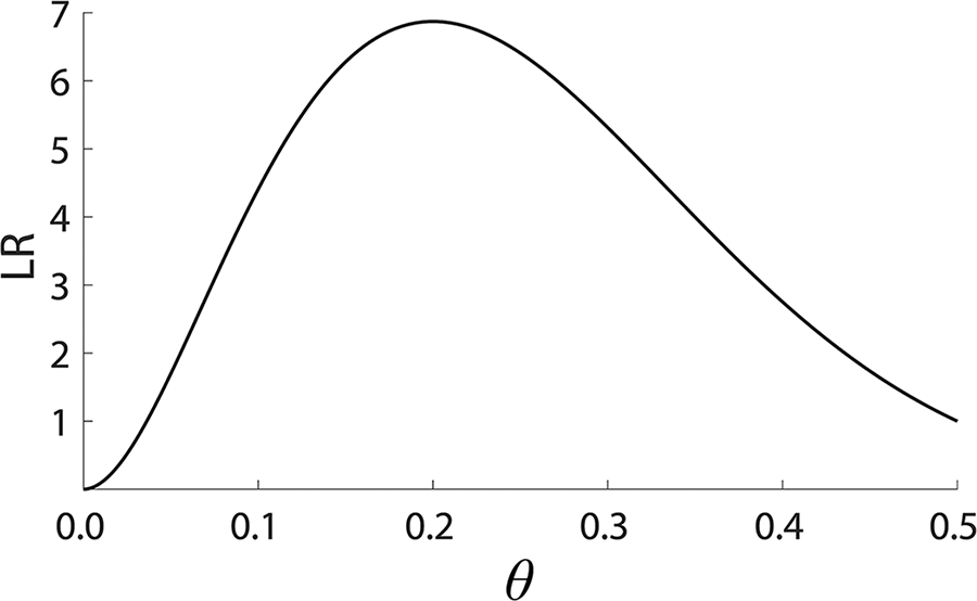Now the LR is a function of θ, not a single number (fig. 1).

Figure 1.

LR as a function of θ for $x=2$, $y=8$.

In practice it seems that what is important is not so much the proscription against composite hypotheses but rather the prescription for how they may be interpreted. We can graph the LR as a function of θ, as if we were admitting composite hypotheses, but we can only make statements like “$\theta =0.2$ is supported over $\theta =0.5$, on given data, by $\mathrm{LR}=6.9$,” while “$\theta =0.1$ is supported over $\theta =0.5$, on those same data, by $\mathrm{LR}=4.4$.”Footnote ⁵ But as a practical matter, the graph is not a sufficiently concise summary for general scientific applications. We still need some way to reduce the function LR(θ) to a single number summarizing the strength of the evidence.

And this is where we get into trouble because focus shifts naturally to the maximum LR (MLR), which occurs over the best supported value—the maximum likelihood estimate (MLE)—of θ. Indeed, given that we are only allowed to make statements about one simple hypothesis comparison at a time, the MLR, itself a ratio of two simple likelihoods, appears as the best single constituent LR to use as a summary feature of the LR graph. (Below I consider how relaxing the requirement that hypotheses must be simple frees us up to consider other features.) We have now successfully summarized the function LR(θ) as a single number, the MLR, but this summary is tethered to the MLE. We appear to have answered the question: How well supported is the MLE compared to (one or more individual) alternative values of θ? But that is not the question we asked initially, which was about the evidence.Footnote ⁶

The MLE of θ arrives on the scene as a seemingly innocuous point of special interest, the value that corresponds to the maximum support, but it rapidly takes over, embroiling us in a downward spiral of increasingly perplexing difficulties. One immediate issue with relying on the MLR to summarize the evidence (continuing to focus for ease of discussion on the coin-tossing example, in which maximization occurs only in the numerator of the LR) is that $\mathrm{MLR}\ge 1$: the MLR can only show evidence in favor of the numerator but never in favor of the denominator. This is problematic, like using a thermometer in which the mercury is prevented from receding.

Another problem with the MLR is that it begs the question of measurement scale in a particularly obvious way because its evidential meaning would appear to require some kind of adjustment to compensate for the maximization itself. The more parameters we maximize over (again, for ease of discussion, assuming maximization occurs only in the numerator), the larger the MLR becomes. How are we to separate the portion of the MLR reflecting the evidence from the portion representing an artifact of the process of maximization? It becomes particularly hard to retain the fiction that the numerical value of the maximum LR has some prima facie meaning with respect to the underlying evidence, regardless of the number of parameters over which the LR is maximized.

There is a third, more subtle but at least as damaging, difficulty with summarizing evidence via MLRs. Simple LRs can be multiplied across two data sets, but MLRs cannot be multiplied. Rather, to obtain the MLR based on two sets of data, we first combine the data to find the new MLE, which is a kind of weighted average of the two original MLEs, and then we find the new MLR with respect to this average MLE on the combined data. Now consider a situation in which data set D₁ favors H₂ by some substantial amount, and D₂ also favors H₂ but by a lesser amount. In such situations it is not uncommon for the combined support for H₂ to be less than the original support on D₁ alone. But this is not how evidence behaves: strong evidence for H₂ followed by weaker evidence also supporting H₂ ought to lead to stronger evidence for H₂, not intermediate evidence. (A blood type match following a DNA match does not lessen the evidence that the defendant was at the crime scene.)Footnote ⁷ This means that we cannot in practice differentiate between situations in which new data are truly diminishing the evidence and situations in which the evidence is in fact increasing but the MLR at the average MLE goes down anyway. This tendency of the MLR to “average” across combined data is entirely due to its dependence on the MLE; simple LRs do not share this defect.Footnote ⁸

Of course none of this need surprise unreconstructed evidentialists, who, after all, disavowed composite hypotheses—and therefore any need for maximization—from the start. But then beyond the simplest of examples, we are left with an irreducible graph of the component simple LRs, not a single number. This is true already in single-parameter cases; the problem is only exacerbated in higher dimensions.

There is also the matter of masking the nature of the real problem: by focusing initially only on those situations in which the LR is a single number, we missed Hacking’s measurement question: How do we ensure that this number always ‘means the same’? It is only when we consider composite hypotheses that it becomes clear we were never warranted in the first place in assuming that the face value of the LR for a simple versus simple hypothesis comparison is the evidence. Composite hypotheses force us to think in terms of the LR graph, which, precisely because it is not a single number, immediately raises the issue of which feature(s) of the graph might be relevant to the evidence. Composite hypotheses are crucial, not only because they are scientifically relevant but also because they beg a question all but hidden as long as we focus on simple hypotheses only.

The urge to sidestep the problem of the evidential interpretation of the MLR is the reason evidentialists have been reluctant to admit composite hypotheses into their formalism in the first place. But it is fair to say that they have failed to provide any viable alternative to the MLR as the summary measure of evidence strength in practice. The preoccupation with simple hypotheses has entailed inherent difficulties for the program, and it has also masked a basic underlying calibration issue. The good news, I believe, is that it has also been masking the possibility of a solution.

4. Toward a Solution to the Measurement Calibration Problem

Consider again the coin-tossing experiment and LR(θ) as shown in figure 1. Let us suppose, following the spirit if not the letter of the Law of Likelihood, that all of the evidential information is captured, somehow, in this graph. What feature(s) of the graph should we take as representing the degree of evidence?

The MLR of course is one possibility, but I have already stated some objections to this option. An alternative would be to use the area under the graph (ALR). (Note that this is only possible if we allow ourselves to consider the truly composite hypothesis $\theta <0.5$ because the ALR requires simultaneous consideration of all of the constituent simple hypotheses.)Footnote ⁹ But while we are at it, why not also consider using sets of features of the graph? For instance, the evidence might be a function of both the MLR and the ALR (e.g., their product or their ratio). What we need is a methodology for figuring out which among the many possibilities is the correct one.

The methodology I propose is quite simple, at least to begin with. Let us consider the behavior of candidate evidence measures in situations in which we have clear intuitions regarding the behavior of evidence and see which of our candidate measures behaves like the object of measurement, the evidence. Here I will illustrate using coin-tossing thought experiments to discover patterns of behavior of the evidence with changes in data, considering the evidence that the coin is either biased toward tails or fair. I propose that, perhaps with a little persuasion, I could convince you that the following patterns capture what we mean when we talk about statistical evidence in this context. (Here I summarize the data in terms of n = the number of tosses, and $x/n$ = the proportion of tosses that land heads.)

• i) Evidence as a function of changes in n for fixed $x/n$. For any given value of $x/n$, the evidence increases as n increases. The evidence may favor bias (e.g., if $x/n=0.05$) or no bias (e.g., if $x/n=1/2$), but in either case it gets stronger with increasing n.

• ii) Evidence as a function of changes in $x/n$ for fixed n. If we hold n constant but allow $x/n$ to increase from 0 up to, say, 0.20, the evidence favoring ‘coin is biased’ diminishes: that is, the evidence for bias is stronger, the further $x/n$ is from 1/2. But we have also already noted that when $x/n$ is close to 1/2 the evidence favors ‘coin is fair’. Therefore, as $x/n$ continues to approach 1/2, at some point the evidence will shift to favoring ‘coin is fair’, and from that point, the evidence for ‘coin is fair’ will increase, the closer $x/n$ is to 1/2.

• iii) Rate of evidence change as a function of changes in n for fixed $x/n$. For given $x/n$, as n increases the evidence increases more slowly with fixed increments of data. For example, consider evidence in favor of bias with one additional tail (T), following T, or TT, or TTT. When the number of tails in a row is small (i.e., when there is weak evidence favoring bias), each subsequent T makes us that much more suspicious that the coin is biased. But suppose we have already observed 100 Ts in a row: now one additional T changes our sense of the evidence hardly at all, as we are already quite positive that the coin is not fair.Footnote ¹⁰

• iv) Changes in $x/n$ as a function of changes in n (or vice versa) for fixed evidence. It follows from i and ii that in order for the evidence to remain constant, n and $x/n$ must adjust to one another in a compensatory manner. For example, if $x/n$ increases from 0 to 0.05, in order for the evidence to remain the same n must increase to compensate; otherwise, the evidence would go down, following ii above. By the same token, it is readily verified that if i and ii hold, then as $x/n$ continues to increase, at some point n must begin to decrease in order to hold the evidence constant as the evidence shifts to favoring ‘coin is fair’.

Note that at this point we have not mentioned probability distributions, likelihoods, or parameterization of the hypotheses. These patterns characterize evidence in only a very informal, vague manner. However, by the same token, they exhibit a kind of generality: they derive from our general sense of evidence, from what we mean by statistical evidence before we attempt a formal mathematical treatment of the concept.

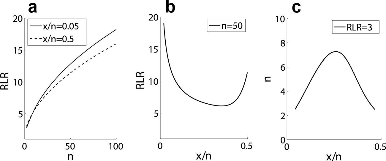
Can we find a precise mathematical expression that exhibits these patterns? As illustrated in figure 2, the ratio $\mathrm{RLR}=\mathrm{MLR}/\mathrm{ALR}$ exhibits all of the expected behaviors. By contrast, neither MLR nor ALR shows all four of these patterns. For instance, MLR, as already noted, cannot show increasing evidence in favor of H₂ because it can never favor H₂ in the first place, and both MLR and ALR increase exponentially in n for fixed $x/n$ rather than showing the concave-down pattern in figure 2a.

Figure 2.

Patterns of behavior of RLR for coin-tossing thought experiments: a, patterns i and iii; b, pattern ii; c, pattern iv.

Of course none of this proves that RLR is the correct, or optimal (or properly calibrated), measure of evidence. But this style of reasoning buys us an important methodological tool. Whichever features of the LR graph we consider and however we combine them, we must be able to show that the resulting evidence measure behaves like the evidence. When proposing candidate evidence measures anything goes, but only those candidates that behave appropriately remain on the ballot. And even in this very simple example, two obvious candidates—the MLR and the ALR—have already dropped out of contention.

Of course, there is no reason to assume that what works in this simple case (i.e., RLR) will work in more complicated cases, nor have we yet resolved the ECP’s fundamental calibration issue. Establishing that a measure behaves like the object of measurement is only a first step, but it is a vital step not previously taken. It provides an “empirical” measurement scale, not an absolute scale, much as early thermoscopes provided good experimental tools while falling short of proper, absolute, calibration (Chang Reference Chang2004).Footnote ¹¹ Projecting an empirical measure onto an absolute scale requires a broader theoretical foundation, but one needs the empirical measure first. My point here is simply that confronting the ECP head on, and in the context of composite hypotheses, opens the door for the first time to the possibility of establishing a proper measurement scale for statistical evidence.

Note too that the coin-tossing exercise suggests the existence of an equation of state involving the three quantities (n, $x/n$, and the evidence), such that fixing any one quantity while allowing a second one to change requires a specific compensatory change in the third. This in turn suggests a new, and potentially very powerful, way to think about the laws governing the behavior of LRs. I am not aware of any evidentialist work that considers such equations, but I see no reason that an evidentialist-at-heart should be prohibited from pursuing their study.

5. Relaxing the Foundations to Include Composite Hypotheses

In order to tackle the ECP in the terms of the preceding section, we need to amend the foundations of evidentialism, but only slightly. I propose the following changes. First, let us retain Edwards’s definition of likelihood, as quoted above, but insert the word “simple” (which is tacit in Edwards’s original statement): “The likelihood, $L\left(H|R\right)$, of a simple hypothesis H given data R, and a specific model, is proportional to $P\left(R|H\right)$, the constant of proportionality being arbitrary.” Second, we can again add the word “simple” to his characterization of a statistical hypothesis: “An essential feature of a simple statistical hypothesis is that its consequences may be described by an exhaustive set of mutually-exclusive outcomes, to each of which a definite probability is attached.” But we can now add a definition of likelihood for a composite hypothesis: “A composite hypothesis H given data R, and a specific model, is the set of all constituent simple hypotheses, defined up to a single constant of proportionality.” Thus, the essential feature of a composite hypothesis is that each of its constituent simple hypotheses may be described by an exhaustive set of mutually exclusive outcomes, to each of which a definite probability is attached. We can now use this definition of a composite hypothesis to define the corresponding composite likelihood, as the set of all constituent simple likelihoods.

Under my proposal, the spirit of the Law of Likelihood can be retained: we can say that all of the evidential information conveyed by given data regarding a comparison between two hypotheses on a particular model is contained in the LR, where, under the expanded definition of hypotheses, the LR is understood to be a function of all unknown parameters, or better still perhaps, a graph. This can equivalently be read as a definition of evidential information, as whatever changes the LR graph.Footnote ¹² But the idea that the (simple) LR itself expresses the degree or weight of the evidence must be abandoned. What I have attempted to argue here is that there is at least the possibility of replacing this notion with something more useful.

6. Discussion

Evidence is a general and vague term in science. Statistical evidence is a narrower concept, but it still inherits some of this vagueness. One way to tackle a general and vague term is by seeking a precise definition that maintains full generality, but of course, this might not be possible. Weyl (Reference Weyl1952, 6) has suggested another approach: “To a certain degree this scheme is typical for all theoretic knowledge: We begin with some general but vague principle, then find an important case where we can give that notion a concrete precise meaning, and from that case we gradually rise again to generality … and if we are lucky we end up with an idea no less universal than the one from which we started. Gone may be much of its emotional appeal, but it has the same or even greater unifying power in the realm of thought and is exact instead of vague.”

Can evidentialism be redeemed and made truly useful to science? Of course I have not proved that the answer is yes. But in section 4 I illustrated a case in which we appear to be able to give the vague concept of statistical evidence a concrete, precise meaning, via the quantity $\mathrm{RLR}=\mathrm{MLR}/\mathrm{ALR}$. Indeed, it appears that it will also be possible to rise again to generality from this first step (Vieland and Seok Reference Vieland and Seok2016).

For those of us who agree with most of what Barnard, Hacking, and Edwards have to say on the subject, it seems worthwhile to see how far we can take this line of reasoning. This also seems to be a singular opportunity for philosophers of science to step into the breach and at least try to solve a problem that has long stood between one of the needs of science—for well-behaved quantitative measures of evidence—and the capabilities of conventional statistical methodologies.