





1. Introduction
In the ocean, surface gravity waves are inherently three dimensional, composed of interacting frequency and directional components. Owing to this three-dimensionality, ocean waves can exceed the classical breaking threshold steepness for two-dimensional (2-D) long-crested waves –
 $ak=0.44$
(with
 $a$
and
 $k$
denoting wave amplitude and wavenumber) in Stokes (Reference Stokes1847) and
 $H_D/L_F=0.142$
(with
 $H_D$
and
 $L_F$
denoting the deep-water wave height and the finite-amplitude deep-water wavelength) in Miche (Reference Miche1944). These three-dimensional (3-D) effects lead to distinct breaking patterns (McAllister et al. Reference McAllister, Draycott, Adcock, Taylor and van den Bremer2019) and existing wave breaking criteria are not valid in highly spread conditions (see, e.g. Kanehira et al. Reference Kanehira, McAllister, Draycott, Nakashima, Taniguchi, Ingram, van den Bremer and Mutsuda2021). In McAllister et al. (Reference McAllister, Draycott, Calvert, Davey, Dias and van den Bremer2024) it was shown that for highly directionally spread wave conditions, breaking onset does not occur until the wave steepness is over double the unidirectional counterpart. Accounting for this three-dimensionality is therefore essential for understanding wave-energy dissipation, air–sea momentum exchange and the loading or response of offshore systems in realistic conditions. Wave breaking behaviour in nature lies between two limiting cases: unidirectional waves with infinitely long crests (no directional spreading) and axisymmetric waves (maximum directional spreading) as described in McAllister et al. (Reference McAllister, Draycott, Davey, Yang, Adcock, Liao and van den Bremer2022) (hereafter referred to as MC22). The axisymmetric focused wave thus provides a simplified yet physically relevant model for studying the essential hydrodynamics of 3-D breaking behaviour in its most extreme form. Axisymmetric focusing and the ensuing jet formation occur across a wide range of scales and regimes (Basak et al. Reference Basak, Farsoiya and Dasgupta2021) – from Faraday jets generated by parametric resonance in vibrating containers (Miles Reference Miles1984) to Worthington jets formed by droplet or disc impacts (Worthington & Cole Reference Worthington and Cole1897; Eggers & Villermaux Reference Eggers and Villermaux2008; Truscott et al. Reference Truscott, Epps and Belden2014). More recently, similar axisymmetric focusing has been experimentally reproduced for gravity waves through linear dispersive focusing by McAllister et al. (Reference McAllister, Draycott, Davey, Yang, Adcock, Liao and van den Bremer2022). Despite differences in the relative importance of gravity, surface tension and viscosity, these processes display similar dynamics across scales, and such jet formation may represent a fundamental feature of free-surface flows (Longuet-Higgins Reference Longuet-Higgins1983).
The theoretical understanding of axisymmetric standing waves and jet formation has evolved over the past decades. Following the third-order theory for axisymmetric standing waves derived by Mack (Reference Mack1962), the first analytical model for jet formation was proposed by Longuet-Higgins (Reference Longuet-Higgins1983) (hereafter also referred to as LH83), who obtained a time-dependent inviscid solution of the Laplace equation with a free surface in the form of a Dirichlet hyperboloid. Subsequent developments, including the asymptotic analysis of Ockendon & Ockendon (Reference Ockendon and Ockendon2024) and the non-perturbative potential-flow theory of Wilkinson et al. (Reference Wilkinson, Morgan and Wilkinson2025), further refined the theoretical framework, elucidating pressure-driven jet initiation and the smooth hyperbolic evolution of the axisymmetric free surface. Since axisymmetric focusing concentrates flow toward the axis from all radial directions, the maximum impact pressure is expected to be significantly higher than in 2-D flip-through events (Lugni et al. Reference Lugni, Brocchini and Faltinsen2006; Martin-Medina et al. Reference Martin-Medina, Abadie, Mokrani and Morichon2018). However, despite indications from large-scale (up to 6 m) vertical jet experiments supporting this expectation, no direct measurements or fully 3-D characterisations of the pressure field at jet onset are available. Under inertia-dominated conditions, the experiments of McAllister et al. (Reference McAllister, Draycott, Davey, Yang, Adcock, Liao and van den Bremer2022) showed that the jet height follows a pre-jet cavity scaling closely related to the
 $H(H/L)^2$
law of Ghabache et al. (Reference Ghabache, Séon and Antkowiak2014), where
 $H$
and
 $L$
denote the cavity depth and lateral extent, respectively. Recent laboratory experiments by Fillette et al. (Reference Fillette, Fauve and Falcon2022) also examined axisymmetric gravity–capillary standing waves and reported that the maximum wave steepness saturates at
 $5/(2\pi )$
under large forcing.
Recent studies have shown that the limiting waveform and critical crest angle of 2-D standing waves remain an open question. Penney & Price (Reference Penney and Price1952) argued that the downward acceleration of the free surface cannot exceed
 $-g$
, implying a limiting crest angle of
 $90^\circ$
, a conclusion later supported by the experiments of Taylor (Reference Taylor1953). In contrast, Longuet-Higgins (Reference Longuet-Higgins1994) proposed a different dynamical mechanism, suggesting that a self-similar superposition of short-wave components could lead to a blow-up of curvature and Lagrangian particle acceleration near the crest. High-resolution computations by Wilkening (Reference Wilkening2011) further indicated that large-amplitude standing waves do not converge to a unique limiting form; instead, high-frequency oscillations emerge near the crest, breaking the expected self-similarity. These results collectively suggest that even in two dimensions the existence of a universal limiting waveform remains unresolved, and that the fundamental criteria for the breaking threshold are still unclear.
Regarding axisymmetric waves, Longuet-Higgins (Reference Longuet-Higgins1983) predicted that once a jet is initiated its shape evolves hyperbolically, and that axisymmetric standing waves should break when the jet angle reaches
 $2\arctan \sqrt 2$
(i.e.
 $109.47^\circ$
). However, as noted in McAllister et al. (Reference McAllister, Draycott, Davey, Yang, Adcock, Liao and van den Bremer2022), identifying the onset of breaking in axisymmetric standing waves is particularly challenging. Unlike progressive waves, overturning cannot be used as an unambiguous indicator, because both wave motion and jet formation involve vertical displacements of the free surface, making the two processes difficult to distinguish. As a consequence, a clear criterion for the onset of breaking in strongly focused axisymmetric waves has not yet been established. Indeed, while McAllister et al. (Reference McAllister, Draycott, Davey, Yang, Adcock, Liao and van den Bremer2022) confirmed that the jet angles in axisymmetric focusing waves follow the Longuet-Higgins (Reference Longuet-Higgins1983) model, experimental limitations prevented verification near the predicted critical angle. Thus, significant uncertainty remains regarding the onset of breaking.
The formation and collapse of cavities generated by the impact of disks, droplets and other bodies have been extensively studied (Truscott et al. Reference Truscott, Epps and Belden2014). The resulting cavity shape depends strongly on the impactor geometry, wettability and impact velocity. It has also been shown by Glasheen & McMahon (Reference Glasheen and McMahon1996) that the non-dimensional pinch-off time
 $\tau =t\sqrt {2g/D}$
, where
 $t$
is the physical pinch-off time,
 $g$
is gravitational acceleration and
 $D$
is a characteristic length scale, remains nearly constant over a broad range of conditions, suggesting the possibility of temporally self-similar collapse (Truscott & Techet Reference Truscott and Techet2009). Moreover, Gekle et al. (Reference Gekle, Gordillo, van der Meer and Lohse2009) demonstrated that the emergence of the high-speed Worthington jet does not originate from a purely local singularity at the pinch-off point. Rather, it is driven by the global collapse of the cavity wall and the associated focusing of kinetic energy, implying that a full understanding of jet formation requires analysing the dynamics of the entire collapsing cavity. Despite these advances, the cavity shape and collapse induced by a continuously falling primary jet remain poorly understood. While studies on cavities formed by a liquid column freely falling onto a quiescent free surface exist (Kersten et al. Reference Kersten, Ohl and Prosperetti2003), the cavity dynamics driven by a continuously falling primary jet have not been directly studied to date.
High-resolution computational fluid dynamics models have further advanced our understanding of jet formation. Duchemin et al. (Reference Duchemin, Popinet, Josserand and Zaleski2002) directly solved the Navier–Stokes equations and reproduced bubble-bursting jets for the first time. More recent axisymmetric simulations employing interface-capturing techniques such as the coupled level-set and volume-of-fluid method have systematically examined the roles of viscosity, inertia and surface tension in determining jet shape, speed and scaling (Castillo-Orozco et al. Reference Castillo-Orozco, Davanlou, Choudhury and Kumar2015; Farsoiya et al. Reference Farsoiya, Mayya and Dasgupta2017; Ismail et al. Reference Ismail, Gañán-Calvo, Castrejón-Pita, Herrada and Castrejón-Pita2018; Blanco–Rodríguez & Gordillo Reference Blanco–Rodríguez and Gordillo2020). However, the dynamics leading to a secondary jet remain poorly understood. Most existing theoretical and numerical studies terminate their analysis once the primary jet has been launched, and, to the authors’ knowledge, experimental observations of secondary jets are absent. From the large-scale measurements of McAllister et al. (Reference McAllister, Draycott, Davey, Yang, Adcock, Liao and van den Bremer2022), it is evident that the primary jet generates a secondary cavity whose pinch-off produces a strong acoustic impulse not observed during the formation of the initial jet (see, e.g. supplementary movie 7 in McAllister et al. (Reference McAllister, Draycott, Davey, Yang, Adcock, Liao and van den Bremer2022)). Grumstrup et al. (Reference Grumstrup, Keller and Belmonte2007), Yu et al. (Reference Yu, Zong and Zhang2023) also showed that cavity pinch-off generates a sharp acoustic burst, manifested as surface ripples and strong acoustic emissions during rapid cavity collapse. Although the present study does not resolve the gas phase or acoustic propagation, Francoeur et al. (Reference Francoeur, Matoza, Ortiz and De Negri2025) and Nelli et al. (Reference Nelli, Tothova, Ooi and Manasseh2025) have demonstrated the potential of acoustic emission to infer breaking intensity, highlighting the importance of understanding gas entrainment and strength of cavity collapse (Deike Reference Deike2022). Furthermore, the primary cavity collapse can strongly modify the subsequent free-surface evolution. Rabbi et al. (Reference Rabbi, Speirs, Kiyama, Belden and Truscott2021) conducted water entry experiments using two spheres falling in a tandem configuration. Their results showed that the impact force on the trailing sphere is determined by the timing between the first cavity’s pinch-off and the second sphere’s arrival at the free surface. These findings indicate that it is insufficient to consider only the jet generated at the primary collapse; rather, the entire sequence of post-collapse free-surface dynamics must be evaluated to understand the full progression toward secondary-jet formation. Therefore, accurately characterising the four-stage post-primary collapse sequence – the primary-jet impact, the subsequent cavity formation, its pinch-off and collapse, and the re-emergence of a secondary jet – is essential. Such analysis not only advances the fundamental understanding of axisymmetric breaking but also provides crucial insight into the underlying fluid mechanics governing impact pressures, air entrainment and associated acoustic phenomena.
(a) Comparison between the experimental axisymmetric jet profile and the circular-basin SPH simulation (Kanehira et al. Reference Kanehira, Mutsuda, Doi, Taniguchi, Draycott and Ingram2019), showing that SPH underestimates the jet height and fails to reproduce the sharp jet tip. (b) Conceptual diagram of the OceanSPHysics3D framework, in which a fully nonlinear potential-flow (FNPF) domain solves the large-scale wave propagation, while an embedded local SPH subdomain resolves wave breaking. The two solvers exchange information through the overlap region
 $\varOmega _{ov\textit{erlap}}$
.

To address this gap, we develop a fully 3-D numerical framework capable of resolving 3-D wave breaking problems, including, as studied here, axisymmetric jet formation and post-collapse dynamics. Mesh-free methods such as smoothed particle hydrodynamics (SPH) (Gingold & Monaghan Reference Gingold and Monaghan1977; Lucy Reference Lucy1977) and moving particle semi-implicit (Koshizuka & Oka Reference Koshizuka and Oka1996), which naturally accommodate strongly deformed free surfaces, have therefore been widely applied to breaking-wave problems (Altomare et al. Reference Altomare, Scandura, Cáceres, van der A and Viccione2023; King et al. Reference King, Lind, Rogers, Stansby and Vacondio2023). However, as illustrated in figure 1(a), resolving highly localised breaking without excessive dissipation or cost is still difficult in a 3-D domain (see also Kanehira et al. Reference Kanehira, Mutsuda, Doi, Taniguchi, Draycott and Ingram2019, Reference Kanehira, McAllister, Draycott, Nakashima, Taniguchi, Ingram, van den Bremer and Mutsuda2021). Coupled frameworks (Narayanaswamy et al. Reference Narayanaswamy, Crespo, Gómez-Gesteira and Dalrymple2010; Oger et al. Reference Oger, Le Touzé, Ducrozet, Candelier and Guilcher2014; Sriram et al. Reference Sriram, Ma and Schlurmann2014; Fourtakas et al. Reference Fourtakas, Stansby, Rogers, Lind, Yan and Ma2017; Altomare et al. Reference Altomare, Tagliafierro, Dominguez, Suzuki and Viccione2018; Verbrugghe et al. Reference Verbrugghe, Domínguez, Crespo, Altomare, Stratigaki, Troch and Kortenhaus2018; Marrone et al. Reference Marrone, Le Touzé, Colagrossi and Di Mascio2026) offer a promising route forward, but existing SPH-based schemes often rely on particle creation/deletion for free-surface tracking, limiting their applicability to multidirectional seas. No current framework addresses fully 3-D coupling with arbitrary incident wave directions (Liu et al. Reference Liu, Liu, Li, Chen, Chen, Arikawa and Shi2023). These challenges motivate the present development of OceanSPHysics3D, a fully 3-D coupling system that integrates high-fidelity wave information from the fully nonlinear potential-flow solver OceanWave3D (Engsig-Karup et al. Reference Engsig-Karup, Bingham and Lindberg2009) with the graphics processing unit (GPU)-accelerated SPH solver DualSPHysics (Domínguez et al. Reference Domínguez2022) as illustrated in figure 1(b). In this work, we employ OceanSPHysics3D to resolve, for the first time, the entire sequence of axisymmetric wave breaking in fully three dimensions – including primary-jet formation, free-fall and cavity evolution, violent pinch-off and secondary-jet formation – thereby bridging long-standing gaps in the physical understanding of this phenomenon.
In this study, our aim is to develop a unified physical description of the entire sequence of axisymmetric wave breaking – from primary-jet formation to free-fall, secondary cavity formation and collapse and the emergence of the secondary jet – by analysing the associated pressure forcing, jet kinematics, cavity self-similarity and secondary-jet morphology. To guide our investigation, we focus on the following questions: (i) What is the 3-D pressure field responsible for primary-jet formation, and what is its peak magnitude? (ii) Can the critical crest-angle criterion of Longuet-Higgins (Reference Longuet-Higgins1983) reliably indicate breaking onset when assessed through jet kinematics and acceleration? (iii) How does the cavity collapse evolve after jet impact, and does it follow or deviate from classical self-similar scaling? (iv) What mechanisms govern the formation and bifurcation behaviour of the secondary jet? The remainder of this paper is organised as follows. Section 2 introduces the OceanSPHysics3D framework and the implementation of the open-boundary coupling strategy. Section 3 presents the validation against axisymmetric focused wave experiments, together with the numerical set-up and convergence tests. Section 4 addresses the questions posed above through a detailed analysis of primary- and secondary-jet formation, cavity dynamics and the applicability of the critical crest-angle criterion. The main physical insights are summarised in § 5.
2. Numerical methods
2.1. Nonlinear potential flow
The present study employs OceanWave3D (Engsig-Karup et al. Reference Engsig-Karup, Bingham and Lindberg2009), a fully nonlinear potential-flow solver, to simulate wave evolution away from breaking. The potential-based formulation offers a computationally efficient alternative to solving the full Navier–Stokes equations while retaining the essential nonlinear wave dynamics including wave dispersion and nonlinear wave–wave interactions with high accuracy, but excluding viscous effects.
2.1.1. Governing equations
We consider a Cartesian coordinate system in which the
 $xy$
-plane coincides with the still-water surface, and the vertical
 $z$
axis is oriented upwards. The free-surface elevation at time
 $t$
is given by
 $z = \eta (\boldsymbol{x}, t)$
, where
 $\boldsymbol{x} = (x, y)$
denotes the horizontal position vector. Assuming that the fluid is incompressible and irrotational, a velocity potential
 $\phi (\boldsymbol{x},z,t)$
exists such that
 \begin{align} \boldsymbol{u} = \boldsymbol{\nabla }\phi = (\phi _x,\phi _y,\phi _z), \end{align}
and the incompressibility condition
 $\boldsymbol{\nabla }\boldsymbol{\cdot }\boldsymbol{u}=0$
reduces to the Laplace equation
 \begin{align} {\nabla} ^2 \phi = 0 \quad \text{for } -h \leq z \lt \eta , \end{align}
where
 $h(\boldsymbol{x})$
denotes the constant still-water depth (
 $h(\boldsymbol{x})=\text{const}$
). Equations (2.1) and (2.2) constitute the governing equations for the potential-flow formulation used in OceanWave3D.
2.1.2. Boundary conditions and coordinate transformation
The kinematic and dynamic boundary conditions for potential flow are expressed as
 \begin{align} \partial _t \eta = -\boldsymbol{\nabla }\eta \boldsymbol{\cdot }\boldsymbol{\nabla }\tilde {\phi } + \tilde {w} (1 + \boldsymbol{\nabla }\eta \boldsymbol{\cdot }\boldsymbol{\nabla }\eta ), \\[-28pt] \nonumber \end{align}
 \begin{align} \partial _t \tilde {\phi } = -g \eta - \frac {1}{2} \big ( \boldsymbol{\nabla }\tilde {\phi } \boldsymbol{\cdot }\boldsymbol{\nabla }\tilde {\phi } - \tilde {w}^2 (1 + \boldsymbol{\nabla }\eta \boldsymbol{\cdot }\boldsymbol{\nabla }\eta ) \big ), \\[0pt] \nonumber \end{align}
where
 $\tilde {\phi } = \phi (\boldsymbol{x}, z = \eta , t)$
denotes the velocity potential and
 $\tilde {w} = \partial _z \phi |_{z = \eta }$
represents the vertical velocity, both evaluated at the free surface. These conditions are expressed in the Zakharov form (Zakharov Reference Zakharov1968). The horizontal gradient operator is defined as
 $\boldsymbol{\nabla }= (\partial _x, \partial _y)$
and
 $g$
is the gravitational acceleration. To numerically integrate (2.3) and (2.4), initial conditions for both
 $\eta (\boldsymbol{x}, 0)$
and
 $\tilde {\phi }(\boldsymbol{x}, 0)$
must be specified. In this study the initial conditions are obtained from linear wave theory, specified at a time
 $t_0=-11$
s when the wave group is sufficiently dispersed and remains approximately linear as in McAllister et al. (Reference McAllister, Draycott, Davey, Yang, Adcock, Liao and van den Bremer2022). To advance (2.3) and (2.4) in time, the Laplace equation (2.2) is solved within the fluid domain subject to the following boundary conditions:
 \begin{align} \phi = \tilde {\phi } \quad \text{at } z = \eta , \\[-28pt] \nonumber \end{align}
 \begin{align} \partial _z \phi + \boldsymbol{\nabla }h \boldsymbol{\cdot }\boldsymbol{\nabla }\phi = 0 \quad \text{at } z = -h. \\[0pt] \nonumber \end{align}
After solving (2.2), the vertical velocity
 $\tilde {w}$
at the free surface is obtained, and the time evolution of
 $\eta$
and
 $\tilde {\phi }$
is computed using (2.3) and (2.4).
To transform the physical domain with a moving free surface into a fixed computational domain, the
 $\sigma$
coordinate system is introduced as
 \begin{align} \sigma \equiv \frac {z + h(\boldsymbol{x})}{\eta (\boldsymbol{x}, t) + h(\boldsymbol{x})} \equiv \frac {z + h(\boldsymbol{x})}{d(\boldsymbol{x}, t)}, \end{align}
where
 $d(\boldsymbol{x}, t) = \eta (\boldsymbol{x}, t) + h(\boldsymbol{x})$
is the total instantaneous water depth. This transformation maps the time-dependent vertical domain
 $[-h(\boldsymbol{x}), \eta (\boldsymbol{x}, t)]$
to the fixed interval
 $[0, 1]$
. In the vertical direction, grid points are non-uniformly distributed using a grid clustering technique in Engsig-Karup et al. (Reference Engsig-Karup, Bingham and Lindberg2009). This set-up intentionally clusters the vertical grid steps near the free surface to achieve finer spatial resolution. The governing equations are discretised using sixth-order central finite differences in all spatial directions and integrated in time using a classical fourth-order Runge–Kutta scheme. For further details on the numerical solution, the reader is referred to Engsig-Karup et al. (Reference Engsig-Karup, Bingham and Lindberg2009).
2.2. Smoothed particle hydrodynamics
2.2.1. Smoothed particle hydrodynamics formulation
The particle-based SPH solver, DualSPHysics version 5.2 (Domínguez et al. Reference Domínguez2022), used in this study follows the SPH formulation (Gingold & Monaghan Reference Gingold and Monaghan1977; Lucy Reference Lucy1977). Physical quantities are approximated through kernel interpolation over neighbouring particles. For comprehensive reviews of the SPH methodology and its applications in fluid dynamics, readers are referred to Violeau & Rogers (Reference Violeau and Rogers2016), Le Touzé & Colagrossi (Reference Le Touzé and Colagrossi2025), Gotoh & Khayyer (Reference Gotoh and Khayyer2025). In the SPH framework, the physical quantities (
 $\phi (\boldsymbol{r})$
) at a calculation point
 $\boldsymbol{r}$
are first approximated using an integral interpolation, i.e.
 \begin{align} \phi (\boldsymbol{r}) = \int _\varOmega \phi (\boldsymbol{r}') W \big(\|\boldsymbol{r} - \boldsymbol{r}'\|, h_{\textit{SPH}} \big) \, {\rm d}\boldsymbol{r}', \end{align}
where
 $W$
is the smoothing kernel with compact support, meaning that its value is non-zero only within a finite radius proportional to the smoothing length
 $h_{\textit{SPH}}$
. Here,
 $\boldsymbol{r}'$
denotes a neighbouring position vector in the kernel support and
 $\varOmega$
is the integration region. This integral is then discretised into a summation over particles as
 \begin{align} \phi (\boldsymbol{r}_i) \approx \sum _j^N \phi (\boldsymbol{r}_{\kern-1pt j}) W \big(\|\boldsymbol{r}_i - \boldsymbol{r}_{\kern-1pt j}\|, h_{\textit{SPH}} \big)V_j , \end{align}
where
 $V_{j}={m_{\kern-1pt j}}/{\rho _j}$
is the volume of neighbouring particle
 $j$
, with
 $m_{\kern-1pt j}$
its mass and
 $\rho _j$
its density, and
 $N$
denotes the total number of particles. Using this SPH interpolation, the gradient of physical quantities (
 $\phi (\boldsymbol{r_i})$
) can be expressed as
 \begin{align} \boldsymbol{\nabla} _i \phi (\boldsymbol{r}_i) = \sum _j^N \phi (\boldsymbol{r}_{\kern-1pt j}) \boldsymbol{\nabla} _i W_{\textit{ij}} {V_j}, \end{align}
where
 $W_{\textit{ij}}= W(\|\boldsymbol{r}_i - \boldsymbol{r}_{\kern-1pt j}\|, h_{\textit{SPH}})$
. Other expressions for gradients are also used (see Violeau & Rogers Reference Violeau and Rogers2016). Using this numerical operator, the governing equations of the fluid are discretised as SPH particles. The kernel function used in this paper is the Wendland kernel (Wendland Reference Wendland1995) which is expressed as
 \begin{align} W(q,h)= \begin{cases} \alpha _D\,\left (1-\dfrac {q}{2}\right )^{4}\,(2q+1), & 0 \le q \le 2,\\[9pt] 0, & 2\lt q, \end{cases} \end{align}
where
 $q={r}/{h}={\| \boldsymbol{r}_i-\boldsymbol{r}_{\kern-1pt j}\|}/{h}$
,
 $\alpha _{D}$
is the normalisation constant, equal to
 ${7}/{4\pi h^{2}}$
in two dimensions and
 ${21}/{16\pi h^{3}}$
in three dimensions.
2.2.2. Governing equations
The SPH discretised form of the governing equations for fluid flow is given below. The continuity equation, including a density diffusion term is written as
 \begin{align} \frac {{\rm d} \rho _i}{{\rm d}t} = \sum _j^N m_{\kern-1pt j} (\boldsymbol{u}_{\kern-1pt j} - \boldsymbol{u}_i) \boldsymbol{\cdot }\boldsymbol{\nabla} _i W_{\textit{ij}} + \delta h_{\textit{SPH}} c_0 \sum _j^N \psi _{\textit{ij}} \boldsymbol{\cdot }\boldsymbol{\nabla} _i W_{\textit{ij}} V_j, \end{align}
where the diffusion term is introduced to suppress spurious density oscillations (Molteni & Colagrossi Reference Molteni and Colagrossi2009). Here,
 $c_0$
is the speed of sound, the
 $\delta$
-SPH coefficient
 $\delta =0.1$
and the second term on the right-hand side is defined according to Fourtakas et al. (Reference Fourtakas, Dominguez, Vacondio and Rogers2019) in which the term
 $\psi _{\textit{ij}}$
can be written as
 \begin{align} \psi _{\textit{ij}} = 2 \left(\rho ^T_{\textit{ji}}-\rho ^H_{\textit{ij}} \right)\frac {\boldsymbol{r}_{\textit{ij}}}{\|\boldsymbol{r}_{\textit{ij}}\|^2}, \end{align}
where the superscripts
 $T$
and
 $H$
denote the total and hydrostatic components, respectively, whose calculation is described in Fourtakas et al. (Reference Fourtakas, Dominguez, Vacondio and Rogers2019). This approach smooths only the dynamic component of the density while excluding the hydrostatic part, and does not require the calculation of density gradients (Antuono et al. Reference Antuono, Colagrossi and Marrone2012). As a result, the correct hydrostatic pressure gradient is preserved in still-water conditions. This makes the method computationally efficient and particularly effective for gravity-dominated flows as considered in this study.
The momentum equation is expressed in an extended SPH formulation as
 \begin{align} \begin{aligned} \frac {{\rm d} \boldsymbol{u}_i}{{\rm d}t} = & - \sum _j m_{\kern-1pt j} \left ( \frac {p_i+p_j}{\rho _i\rho _j} \right ) \boldsymbol{\nabla} _i W_{\textit{ij}} + \boldsymbol{g} \\ & + \sum _j m_{\kern-1pt j} \left ( \frac {4 \nu _0 \boldsymbol{r}_{\textit{ij}} \boldsymbol{\cdot }\boldsymbol{\nabla} _i W_{\textit{ij}}}{(\rho _i + \rho _j)(|\boldsymbol{r}_{\textit{ij}}|^2 + \zeta ^2)} \right ) (\boldsymbol{u}_i - \boldsymbol{u}_{\kern-1pt j}) \\ & + \sum _j m_{\kern-1pt j} \left (\frac {\boldsymbol{\tau }_i+\boldsymbol{\tau }_j}{\rho _i\rho _j} \right ) \boldsymbol{\cdot }\boldsymbol{\nabla} _i W_{\textit{ij}}, \end{aligned} \end{align}
where
 $\boldsymbol{r}_{\textit{ij}} = \boldsymbol{r}_i - \boldsymbol{r}_{\kern-1pt j}$
,
 $\nu _{0}$
is the kinematic viscosity (typically
 $1.0 \times 10^{-6}\,\mathrm{m^{2}\,s^{-1}}$
for water) and
 $\zeta ^{2} = 0.01 h^{2}$
is a small regularisation parameter introduced to avoid singularities. The second term on the right-hand side corresponds to the laminar viscous stresses as formulated in Lo & Shao (Reference Lo and Shao2002). The last term involves
 $\boldsymbol{\tau }$
, which denotes the sub-particle scale (SPS) stress tensor presented in Dalrymple & Rogers (Reference Dalrymple and Rogers2006), which is employed to model the effect of the SPS turbulence associated with wave breaking.
2.2.3. Pressure and time-stepping schemes
Assuming the fluid is weakly compressible, the pressure can be calculated using Tait’s equation of state, which relates pressure to the density, i.e.
 \begin{align} p = b \left [\left (\frac {\rho }{\rho _0}\right )^\gamma - 1\right ] \!, \end{align}
where
 $\gamma = 7$
,
 $b = c_0^2 \rho _0 / \gamma$
,
 $\rho _0 = 1000\,\rm {kg\,m}^{-3}$
is the reference density. This formulation allows explicit computation of pressure, significantly reducing computational costs compared with solving Poisson’s equation with an implicit method. In this study the speed of sound was defined as
 $c_0=20\sqrt {g/k_0}$
based on the phase speed of deep water, where
 $k_0$
denotes the characteristic wavenumber of an axisymmetric standing wave discussed in § 3.2. An explicit second-order time integration method (the symplectic scheme) was employed. The size of time stamps is determined according to Monaghan (Reference Monaghan1992) with a Courant–Friedrichs–Lewy (CFL) number of 0.2.
2.2.4. Boundary conditions
Numerous versions of boundary conditions have been used where SPH applies to the whole domain, effectively as a numerical wave basin (Ni et al. Reference Ni, Feng, Huang, Zhang and Feng2018; Tafuni et al. Reference Tafuni, Domínguez, Vacondio and Crespo2018; Kanehira et al. Reference Kanehira, Mutsuda, Doi, Taniguchi, Draycott and Ingram2019; Verbrugghe et al. Reference Verbrugghe, Domínguez, Altomare, Tafuni, Vacondio, Troch and Kortenhaus2019; Tsuruta et al. Reference Tsuruta, Khayyer, Gotoh and Suzuki2021; Yang et al. Reference Yang, Draycott, Stansby and Rogers2023). Here the SPH domain is embedded within the OceanWave3D domain that covers the entire domain as in figure 1(b); this is equivalent to Chimera meshing for mesh-based methods (Benek et al. Reference Benek, Steger and Dougherty1983), sometimes known as overset meshing in OpenFOAM (OpenCFD Ltd 2017). Buffer zones are initially set up on the boundaries of the SPH domain (figure 2 b) and particles specified as boundary particles are given velocities from the OceanWave3D computation through trilinear interpolation. Unlike conventional schemes that restrict buffer particles to horizontal motion, the present method directly tracks their full 3-D motion, allowing accurate free-surface representation and avoiding spurious vortices near the boundary (Ni et al. Reference Ni, Feng, Huang, Zhang and Feng2018; Kanehira et al. Reference Kanehira, Draycott, Rogers and Stansby2025). The refilling mode used in previous studies (Tafuni et al. Reference Tafuni, Domínguez, Vacondio and Crespo2018; Verbrugghe et al. Reference Verbrugghe, Domínguez, Altomare, Tafuni, Vacondio, Troch and Kortenhaus2019; Yang et al. Reference Yang, Draycott, Stansby and Rogers2023) is disabled, as buffer particles are directly advected by interpolated velocities. Although boundary particles may be gradually lost due to Stokes drift, the buffer region is sufficiently wide for the simulation duration. Pressure is not interpolated, since the weakly compressible SPH formulation is inconsistent with the incompressible OceanWave3D field, which can cause instability. Instead, the horizontal pressure gradient into the inner SPH domain is set to zero, providing stable simulations and close agreement between the overlapping SPH and OceanWave3D results for waves up to moderate steepness. Further details of the DualSPHysics implementation and the coupling procedure are provided in Appendix A. We use the modified dynamic boundary condition (mDBC) by English et al. (Reference English, Domínguez, Vacondio, Crespo, Stansby, Lind, Chiapponi and Gómez-Gesteira2022) for the solid boundaries.
3. Simulated axisymmetric wave and its validation
3.1. Numerical set-up
To demonstrate the proposed framework OceanSPHysics3D in § 2, we simulate an axisymmetric standing wave in the 3-D numerical domain. A temporally and spatially localised standing wave is generated at the centre of the computational domain. The numerical set-up used here corresponds to the experiments in McAllister et al. (Reference McAllister, Draycott, Davey, Yang, Adcock, Liao and van den Bremer2022).
Numerical domain in OceanWave3D (a) and the SPH subdomain (b). The SPH subdomain is highlighted by the blue rectangle in panel (a). The
 $\textrm {WG}_1$
is installed near the open boundary W at (
 $x,y$
) = (
 $-1.384,0$
) and
 $\textrm {WG}_2$
at the centre (
 $x,y$
) = (
 $0,0$
).

The axisymmetric wave is generated through linear dispersive focusing, in which a broad-banded spectrum of axisymmetric components is phase aligned to concentrate energy at the tank centre. As discussed in McAllister et al. (Reference McAllister, Draycott, Davey, Yang, Adcock, Liao and van den Bremer2022), the focusing mechanism is predominantly linear, with nonlinearity only influencing the crest height at focus in the evolution. The limiting steepness of such axisymmetric waves can be characterised by the critical semi-apex angle
 $\gamma _c = \arctan \sqrt {2}=54.7^\circ$
, equivalently corresponding to the full crest angle
 $2\gamma _c=109.47^\circ$
, proposed by Longuet-Higgins (Reference Longuet-Higgins1983), beyond which jet formation occurs.
Figure 2(a) illustrates the initial water free surface in OceanWave3D (
 $t_0=-11$
s) and the SPH subdomain represented by the centrally located vertical rectangular volume. To initialise OceanWave3D, two input fields were prescribed: the velocity potential at the free surface and the free-surface elevation, both generated from linear wave theory. The directional spectrum was set identical to the input spectrum of McAllister et al. (Reference McAllister, Draycott, Davey, Yang, Adcock, Liao and van den Bremer2022), consisting of a uniform directional distribution and the ITTC (International Towing Tank Conference) frequency spectrum (Matthews Reference Matthews1972), with mean period
 $\overline {T} = 2.3$
s. The linear amplitude sum
 $A_0$
was taken directly from McAllister et al. (Reference McAllister, Draycott, Davey, Yang, Adcock, Liao and van den Bremer2022) (table 2). In particular,
 $A_0 = 0.407$
m was used for Exp. 20,
 $A_0 = 1.018$
m for Exp. 50 and
 $A_0 = 1.526$
m for Exp. 75. The frequency spectrum was discretised with
 $\delta f = 1/64 = 0.0156$
Hz, with maximum frequency 2 Hz, consistent with the wavemaker limit in the experiments.
The numerical set-up used in OceanWave3D is listed in table 1. The OceanWave3D domain is
 $100 \times 100$
m with water depth
 $h=2$
m, consistent with simulations presented in McAllister et al. (Reference McAllister, Draycott, Davey, Yang, Adcock, Liao and van den Bremer2022). A coarser horizontal grid (
 $N_x=N_y=513$
) was used instead of
 $N_x=N_y=1024$
in McAllister et al. (Reference McAllister, Draycott, Davey, Yang, Adcock, Liao and van den Bremer2022), since finer grids captured steep jets that caused instability. This numerical instability triggers numerical divergence in the fluid velocity and surface elevation near the centre, prematurely terminating the potential-flow solver just before the time of focusing (as shown in figure 8
i in McAllister et al. (Reference McAllister, Draycott, Davey, Yang, Adcock, Liao and van den Bremer2022)). Therefore, in OceanWave3D, when the vertical acceleration exceeds a specified threshold (e.g.
 $0.4g$
), wave breaking is assumed to occur and a one-dimensional spatial filter is applied to smooth the free surface and suppress numerical divergence. To maintain numerical stability in the 3-D domain, we implemented a localised 2-D Gaussian-like smoothing filter (
 $3 \times 3$
kernel) that is applied when the vertical acceleration exceeds
 $0.4g$
. Since this filter operates on a fixed number of grid points, its physical coverage scales directly with the grid spacing. On the finer grid (
 $N_x=N_y=1024$
) in this study, the physical filtering area becomes too narrow to suppress the rapid growth of steep jets. As our aim is to provide boundary conditions for the SPH subdomain, we employ a coarser resolution rather than adjusting the filtering width; hence, this resolution ensures stability beyond the focusing event. Crucially, this highly localised filtering only attenuates the extreme wave crest near the centre and does not affect the wave profiles near the SPH boundaries (
 $x = \pm 1.5$
m), maintaining very good agreement with the experimental data as shown in figure 6(a). The time step was set to
 $\Delta t_{\textit{FNPF}}=0.04$
s so that the Courant number
 $C_g \Delta t_{\textit{FNPF}} / \Delta x = 0.6$
. The group velocity in finite depth is then given by
 \begin{align} C_g = n \frac {\omega _0}{k_0}, \qquad n = \frac {1}{2}\left (1+\frac {2k_0 h}{\sinh (2k_0 h)}\right ), \end{align}
where
 $\omega _0=\sqrt {gk_0 \tanh (k_0 h)}$
is the angular frequency. The characteristic wavelength was
 $\lambda _0 = 2r_0 = 12.26$
m with the radial position of the wave trough
 $r_0=6.13$
m at linear focus. The simulations started at
 $t_0=-11$
s, ensuring all frequency components had time to propagate across the domain and constructively interfere at
 $t=0$
.
Numerical parameter used in OceanWave3D.

Table 1. Long description
A table comparing numerical parameters used in OceanWave3D. The table has 12 rows and 12 columns. Column headers are: Case, Exp., L0, L1 (m), L0/dp, A0/dp, hSPH/dp, R (hr), MGPU (GB), Np (x10^6), A (m), cIC (m/s^-1). Row 1: Case 1, Exp. 20, L0 3, L1 0.4, L0/dp 150, A0/dp 20, hSPH/dp 1.7, R 6.17, MGPU 1.57, Np 4.0, A 0.338†, cIC 0.456‡. Row 2: Case 2, Exp. 5, L0 5, L1 1, L0/dp 250, A0/dp 51, hSPH/dp 1.7, R 16.7, MGPU 4.31, Np 10.9, A 1.95, cIC 4.65. Row 3: Case 3, Exp. 3, L0 3, L1 1, L0/dp 150, A0/dp 51, hSPH/dp 1.4, R 9.6, MGPU 3.20, Np 6.8, A 2.15, cIC 5.35. Row 4: Case 4, Exp. 50, L0 3, L1 1, L0/dp 150, A0/dp 51, hSPH/dp 1.7, R 13.1, MGPU 3.20, Np 6.8, A 1.680‡, cIC 4.83*. Row 5: Case 5, Exp. 3, L0 3, L1 1, L0/dp 150, A0/dp 51, hSPH/dp 2.0, R 16.4, MGPU 3.20, Np 6.8, A 1.93, cIC 5.09. Row 6: Case 6, Exp. 3, L0 3, L1 1, L0/dp 75, A0/dp 26, hSPH/dp 1.7, R 0.9, MGPU 0.45, Np 0.9, A 1.57, cIC 4.03. Row 7: Case 7, Exp. 3, L0 3, L1 1, L0/dp 100, A0/dp 34, hSPH/dp 1.7, R 2.7, MGPU 1.01, Np 2.1, A 1.60, cIC 4.12. Row 8: Case 8, Exp. 3, L0 3, L1 1.2, L0/dp 150, A0/dp 76, hSPH/dp 1.4, R 12.0, MGPU 3.79, Np 7.7, A 6.19, cIC 10.72. Row 9: Case 9, Exp. 3, L0 3, L1 1.2, L0/dp 150, A0/dp 76, hSPH/dp 1.7, R 15.6, MGPU 3.79, Np 7.7, A 5.16, cIC 10.20. Row 10: Case 10, Exp. 75, L0 3, L1 1.2, L0/dp 150, A0/dp 76, hSPH/dp 2.0, R 19.9, MGPU 3.79, Np 7.7, A 6.02†, cIC 10.38*. Row 11: Case 11, Exp. 3, L0 3, L1 1.2, L0/dp 75, A0/dp 38, hSPH/dp 1.7, R 1.3, MGPU 0.53, Np 1.0, A 3.58, cIC 7.92. Row 12: Case 12, Exp. 3, L0 3, L1 1.2, L0/dp 300, A0/dp 153, hSPH/dp 1.7, R 254.8, MGPU 31.96, Np 59.9, A 6.55, cIC 13.76.
Comparison of the crest amplitudes (
 $A$
) and peak crest velocities (
 $\dot {\eta }_C$
) obtained from the experiments (McAllister et al. (Reference McAllister, Draycott, Davey, Yang, Adcock, Liao and van den Bremer2022)) and SPH simulations. In the experimental data, superscripts
 $\dagger$
and
 $\ddagger$
denote values measured using wave gauges and those obtained from calibrated images. Superscripts
 $I$
and
 $\star$
in
 $\dot {\eta }_C$
indicate velocities derived from calibrated images and from the theoretical expression
 $\dot {\eta }_C = \sqrt {2g(A - A_{{cusp}})}$
, where
 $A_{{cusp}}$
denotes the crest amplitude at the onset of cusp formation. Underlined values are highlighted to aid visual comparison among selected cases; for instance, cases 2 and 4 illustrate the effect of
 $L_0$
, whereas cases 4, 6 and 7 highlight the influence of particle resolution. Here
 $N_{{p}}$
denotes the total number of particles used.

Table 2 Long description
The table compares crest amplitudes (A) and peak crest velocities (ηC) obtained from experiments and SPH simulations. It includes 12 cases with various experimental conditions and simulation parameters. The columns are Case, Exp., L0, L1 (m), L0/dp, A0/dp, hSPH/dp, R (hr), MGPU (GB), Np (×10⁶), A (m), and ηC (m s⁻¹). The rows provide specific values for each case, with some values underlined for visual comparison. The table highlights the effect of different parameters such as L0 and particle resolution on the results. The experiments are denoted by McAllister et al. (2022), and the simulations are labeled as SPH. Superscripts indicate different measurement methods and theoretical expressions used.
Figure 2(b) presents an enlarged view of the SPH subdomain. To record surface elevations near the open boundary W and at the focus centre,
 $\textrm {WG}_1$
and
 $\textrm {WG}_2$
are installed at (
 $x,y$
) = (−1.384, 0) and (
 $x,y$
) = (0, 0), respectively. The domain length
 $L_0$
was chosen to ensure that reflected waves from the open boundaries of the SPH subdomain would not interfere with the breaking phenomena at the centre of the domain. The thickness of the boundary zone
 $L_1$
was selected such that open-boundary particles remain within the zone even under nonlinear effects such as Stokes drift, since particle refilling was not enabled. The four open boundaries (N, E, S, W) were introduced following the configuration of the existing InOut boundary condition (Tafuni et al. Reference Tafuni, Domínguez, Vacondio and Crespo2018), for which the code was modified accordingly in this study. In the coupling zone, boundary particles are driven solely by the predefined velocity and their velocity is not updated by the equations of motion as described in § 2.2.4.
Table 2 summarises the test cases in this study. To demonstrate applicability, three
 $A_0$
values were used corresponding to Exp. 20, 50 and 75. Following McAllister et al. (Reference McAllister, Draycott, Davey, Yang, Adcock, Liao and van den Bremer2022), crest-angle and velocity analysis show that breaking occurs between Exp. 30 and 40. Thus, case 1 (Exp. 20) represents a non-breaking wave, while cases 2–7 (Exp. 50) and cases 8–12 (Exp. 75) correspond to vertically breaking waves with jet formation, Exp. 75 being the largest condition in McAllister et al. (Reference McAllister, Draycott, Davey, Yang, Adcock, Liao and van den Bremer2022). For Exp. 50 (cases 3–5) and Exp. 75 (cases 8–10), the effect of smoothing was tested by varying
 $h_{\textit{SPH}}/d_p=1.4, 1.7$
and
 $2.0$
, where
 $d_p$
denotes the initial particle spacing. A larger ratio increases the spatial extent of the smoothing kernel, resulting in more heavily smoothed physical quantities across the fluid domain. Convergence was also checked by varying
 $A_0/d_p$
(cases 4, 6, 7 for Exp. 50 and cases 9, 11, 12 for Exp. 75). The results of these sensitivity and convergence tests are provided in Appendices B and D. Higher resolution improves agreement with experiments in jet evolution, while insufficient particles (
 $D/d_p\lt 10$
) cause jet instability (
 $D$
is a jet diameter). Smaller
 $h_{\textit{SPH}}/d_p$
enhances jet height. In cases 2 and 4 for Exp. 50, the sensitivity of the SPH domain length
 $L_0$
on the maximum amplitude
 $A$
was investigated. Although a larger computational domain typically promotes numerical dissipation and wave decay in SPH methods, the calculated amplitudes for these cases exhibit the opposite trend. This behaviour likely arises from the combination of the grid resolution used at the interface of the buffer zone and the
 $h_{\textit{SPH}}/d_p$
ratio; the exact resolution requirements for the SPH subdomain warrant further investigation. On the other hand, regarding the minimum required value of
 $L_0$
, a local spatial smoothing is applied near the centre of the domain, when wave breaking is detected in OceanWave3D (see § 3). To ensure that this smoothing effect does not interfere with the boundaries even after the vertical jet forms, while also considering the computational time,
 $L_0 = 3$
m was adopted (see figure 6). In table 2 the maximum jet amplitudes (
 $A$
) and peak crest velocities
 $\dot {\eta }_C$
obtained from the McAllister et al. (Reference McAllister, Draycott, Davey, Yang, Adcock, Liao and van den Bremer2022) experiments and SPH simulations are also presented. In SPH,
 $A$
represents the maximum elevation of the main jet, excluding detached droplets as shown later in figure 9. For the SPH simulations, the crest velocity
 $\dot {\eta }_C$
is evaluated using the forward finite difference,
 $\dot {\eta }_C(t^n)=(\eta _C^{n+1}-\eta _C^{n})/\Delta t,$
where
 $n$
denotes the discrete output time index. It should be noted that identifying the free surface from particle density becomes unreliable when the jet narrows and free-surface fragmentation occurs (as shown in figure 9
c–e). Specifically, unnatural surface fluctuations begin to appear at
 $t = -0.28\text{ s}$
, leading to subsequent fragmentation (see figure 9
c). To explicitly avoid these uncertainties, the evaluation of the velocity strictly relies on the
 $\eta$
data prior to
 $t = -0.28\text{ s}$
for Exp. 75 and
 $t = 0\text{ s}$
for Exp. 50, respectively. Within this regime, prior to the onset of numerical damping in OceanWave3D, the SPH predictions of
 $\eta$
are in excellent agreement with the OceanWave3D results and are highly reliable, as demonstrated in figure 5(d–f).
Sequence of 3-D water free-surface profiles simulated in the SPH for Exp. 50. Panels (a–c) represent curvature collapse to vertical jet evolution, whereas (d–f) show the falling jet, secondary cavity formation and collapse.

Sequence of 3-D water free-surface profiles simulated in the SPH for Exp. 75. Panels (a–c) represent curvature collapse to vertical jet evolution, whereas (d–f) show the falling jet, secondary cavity formation and collapse.

Figure 4. Long description
The image contains six 3-D surface profiles representing the evolution of water free-surface in a simulation. Each panel shows different stages of the process. Panel A: This 3-D surface profile shows the initial stage of curvature collapse at t = -0.52 seconds. The color scale indicates the magnitude of the velocity vector, ranging from 2 to 6 meters per second. Panel B: This 3-D surface profile illustrates the progression towards a vertical jet at t = -0.28 seconds. The color scale here ranges from 2 to 12 meters per second. Panel C: This 3-D surface profile captures the formation of the vertical jet at t = 0 seconds. The color scale ranges from 2 to 8 meters per second. Panel D: This 3-D surface profile shows the falling jet stage at t = 0.92 seconds. The color scale ranges from 0 to 8 meters per second. Panel E: This 3-D surface profile depicts the secondary cavity formation at t = 1.2 seconds. The color scale ranges from 0 to 8 meters per second. Panel F: This 3-D surface profile illustrates the collapse of the secondary cavity at t = 1.44 seconds. The color scale ranges from 0 to 8 meters per second. Each panel provides a snapshot of the dynamic process, highlighting the changes in the water surface over time.
Figure 3 shows time series snapshots of Exp. 50 from the embedded SPH model, capturing the sequence from trough focusing (a) to primary-jet formation (b), jet evolution (c), falling jet (d), secondary cavity (e) and secondary jet (f). Previous studies have used a variety of terms to describe the collapse of the free surface leading to primary-jet formation. Zeff et al. (Reference Zeff, Kleber, Fineberg and Lathrop2000) referred to this process as ‘curvature collapse’ and stated that it is inertia driven. In contrast, Longuet-Higgins (Reference Longuet-Higgins2001) described a similar process that is gravity driven as a ‘collapse of the trough’. Gekle & Gordillo (Reference Gekle and Gordillo2010) examined ‘cavity collapse’ generated by the impact of a rigid body on a free surface. McAllister et al. (Reference McAllister, Draycott, Davey, Yang, Adcock, Liao and van den Bremer2022) used the term ‘curvature collapse’ for the trough focusing and subsequent cavity collapse that leads to primary-jet formation in axisymmetric wave focusing. In the present study we follow McAllister et al. (Reference McAllister, Draycott, Davey, Yang, Adcock, Liao and van den Bremer2022) and use ‘curvature collapse’ for the primary-jet formation. In contrast, the collapse of the deep cavity formed during the free fall of the primary jet can generate a secondary jet, and because the governing mechanism may be fundamentally different from that of the primary-jet formation, we refer to this process as ‘cavity collapse’ (see § 4.2 for details).
Figure 4 illustrates the same sequence for Exp. 75, but with a more slender jet that extends higher before fragmenting into droplets. In panel (e) the falling jet is entrained into the collapsing cavity, and interaction with a secondary jet is evident. For both Exp. 50 and Exp. 75, the maximum velocity occurs during the initial jet formation (panel b) and decreases as the jet develops. The details of jet formation and evolution are further discussed in § 4.1.
3.2. Axisymmetric wave breaking in 3-D domain
The time series of surface elevations for Exp. 20, 50 and 75 are shown in figure 5. Panels (a–c) display results near the open boundary (
 $\textrm {WG}_1$
), while panels (d–f) correspond to the centre of the domain (
 $\textrm {WG}_2$
). Experimental wave-gauge data (blue) are available only for Exp. 20, whereas floating-marker measurements (cyan) are used for Exp. 50 and Exp. 75. Comparisons show good agreement between OceanWave3D (black) and SPH (red) near the open boundary, although amplitudes are slightly overestimated relative to experiments (WG: wave gauges; Q: Qualisys floating markers obtained in McAllister et al. (Reference McAllister, Draycott, Davey, Yang, Adcock, Liao and van den Bremer2022)). This is partly due to imperfect wave generation, since the target amplitude
 $A_0$
from linear theory does not exactly match the realised crest in the laboratory. At the domain centre, OceanWave3D and SPH agree well during the initial stages of wave propagation (panels e,f). However, discrepancies begin to emerge just before
 $t=0$
, as the vertical acceleration at the focusing point exceeds the threshold (
 $0.4g$
), triggering the application of numerical damping. As the simulation approaches
 $t=0$
, OceanWave3D cannot recreate wave breaking (i.e. vertical jet) and cavity collapse, which could cause reflected waves when its output is used as a boundary input. The domain was therefore chosen to be sufficiently large to avoid interference with the central region of interest. In panels (e,f) the trough deepens after
 $t=0$
s due to secondary cavity formation (figures 3
e and 4
e). It should be noted that the value of
 $\eta$
in figure 5 is not the amplitude of the jet itself. The SPH quantity plotted here is a free-surface elevation calculated from particle density (evaluating the density distribution at various vertical
 $z$
positions for a given location to detect the water elevation at a threshold of 0.5
 $\rho _0$
), and therefore reflects an SPH-based surface measure rather than the peak jet height. Since the slender jet contains relatively few particles, this calculated elevation does not represent the true jet amplitude in the SPH subdomain.
Time series comparison of water surface elevation. Panels (a–c) show the surface elevations measured near the open boundary (
 $x=-1.37$
), while panels (d–f) show the surface elevations at the centre of the simulation domain (
 $x,y=0$
). Here WG denotes the wave-gauge measurements and Q denotes the Qualisys floating-marker measurements.

Comparison of water surface profiles during the development of a vertical jet in Exp. 75. Panel (a) shows the time evolution of surface elevations from the wave trough to the formation of the vertical jet, comparing experimental measurements, OceanWave3D and SPH results at multiple time instants. Panels (b) and (c) present a side view of the free-surface profile at
 $t=0.2$
and
 $t= 0.28$
s, with the latter corresponding to the instant when maximum jet height is observed in the experiment. Here WG denotes the wave-gauge measurements, Q denotes the Qualisys floating-marker measurements and ‘Img.’ denotes the calibrated image-based surface-elevation data.

Figure 6 illustrates the development of the vertical jet in Exp. 75. Panel (a) presents the temporal evolution of radial surface profiles from the initial wave trough to the jet evolution. The results demonstrate that both OceanWave3D and SPH closely follow the experimental measurements (WG, Q and Img.: calibrated high-speed images in McAllister et al. (Reference McAllister, Draycott, Davey, Yang, Adcock, Liao and van den Bremer2022)) during the axisymmetric focusing to vertical jet formation. As the vertical jet develops, OceanWave3D increasingly underestimates the peak elevation due to the application of its spatial filtering, whereas SPH continues to capture the jet growth with high accuracy. Panels (b,c) in figure 6 show side views of the SPH output free surface overlaid onto calibrated image data, with the colour scale representing the vertical velocity
 $w$
. Colouring by vertical velocity reveals the axial stretching of the jet, with upward motion persisting only near the jet tip in panel (c), while the surrounding fluid has already reversed to downward motion. As a result, the jet is stretched into a slender, conical shape (figure 4
d). It is notable that the presented method accurately reproduces the steep wave profile, including the vertical jet. These comparisons highlight the capability of the approach to capture the strongly nonlinear dynamics associated with vertical jet formation and breaking.
The comparison of maximum wave crest velocity defined by
 $\dot {\eta }_C$
and wave amplitude
 $A=\text{max}(\eta _C)$
between experiments and SPH simulations is summarised in table 2. A sensitivity test was first conducted with respect to the horizontal domain length
 $L_0$
in figure 2(b), by comparing case 2 (
 $L_0=5$
) and case 4 (
 $L_0=3$
) under otherwise identical conditions. The resulting maximum wave amplitude
 $A$
differed by approximately 14.9
 $\,\%$
for case 2 and 8.9
 $\,\%$
for case 4 relative to the experimental measurements, while the computational cost did not show a significant variation. Since a higher particle resolution was required in Exp. 75, we adopted
 $L_0=3$
for the remaining cases. Additional sensitivity tests on the particle resolution
 $A_0/d_p$
and the smoothing-length ratio
 $h_{\textit{SPH}}/d_p$
revealed that smaller
 $h_{\textit{SPH}}/d_p$
values (e.g. 1.4) tend to yield slightly larger peak amplitudes and velocities, as local interpolation of velocity and pressure becomes less smoothed compared with larger
 $h_{\textit{SPH}}/d_p$
. However, as shown in Appendix D, excessively small
 $h_{\textit{SPH}}/d_p$
values also caused segmentation of the jet, and thus,
 $h_{\textit{SPH}}/d_p=1.7$
was selected as the representative value. Compared with the experimental data (McAllister et al. (Reference McAllister, Draycott, Davey, Yang, Adcock, Liao and van den Bremer2022)), the SPH results for cases 1, 4 and 12 slightly overestimated both the crest amplitude and peak crest velocity, mainly due to differences between the target and actual incident wave conditions in the experiments. Nevertheless, the SPH simulations reproduced the overall trends with good fidelity, confirming the validity of the present numerical approach. In terms of computational cost, the present coupling approach reduced the run time and memory usage by approximately 90 % compared with the conventional full-basin SPH simulation (Kanehira et al. Reference Kanehira, Mutsuda, Doi, Taniguchi, Draycott and Ingram2019), while maintaining comparable accuracy. Even at
 $d_p=1$
cm, however, the computational expense remained substantial, highlighting the difficulty of performing large numbers of high-resolution single-SPH simulations.
4. Jet formation and post-breaking behaviour
By capitalising on the results of high-fidelity computations presented in § 3.2, we carry out a detailed analysis of the vertical wave breaking dynamics. Section 4.1 focuses on the onset and evolution of jet formation, whereas § 4.2 investigates the post-breaking cavity formation, its subsequent collapse and the mechanism by which the secondary jets are generated.
4.1. Pre-jet curvature collapse and primary-jet evolution
Temporal evolution of the normalised wave-induced pressure (a–d) and the vertical velocity component (e–h) during the formation of the vertical jet in Exp. 75. The black arrows indicate instantaneous velocity vectors.

As reported in McAllister et al. (Reference McAllister, Draycott, Davey, Yang, Adcock, Liao and van den Bremer2022), a highly localised jet is formed as the linear superposition of incident wave components increases in amplitude. Our simulations presented in figures 3 and 4 clearly capture the development of a vertical jet at the wave crest. Comparable jets have also been observed in standing waves and in the so-called ‘flip-through’ wave breaking in front of a vertical wall (Lugni et al. Reference Lugni, Brocchini and Faltinsen2006).
In each of these cases, rapid collapse is the key factor in jet formation, and the pressure impulse theory (Cooker & Peregrine Reference Cooker and Peregrine1995) can be applied to explain the resulting localised jet. However, this theory is valid only during an exceedingly brief instant, for example, when a steep wave front impacts a vertical wall. In contrast, the present study considers a focused wave produced by the axisymmetric convergence of multiple wave frequency components. Under such conditions, the free surface evolves continuously in both time and space up to the point of jet formation; therefore, the impulsive approximation may no longer be applicable.
Instead, we investigate jet formation by tracing how wave-induced pressure gradients drive the flow and transfer energy into fluid motion. Following the analysis of Wilkinson et al. (Reference Wilkinson, Morgan and Wilkinson2025) and consistent with the physical transitions described by Eggers & Villermaux (Reference Eggers and Villermaux2008), the evolution of a free-surface jet can be conceptually divided into three successive phases: (I) a pressure-dominated phase, in which strong pressure gradients accelerate the surface upward and dominate the dynamics; (II) an inertia-dominated phase, where the pressure gradients rapidly vanish and the jet evolves ballistically under its own momentum; and (III) a gravity–capillary phase, in which the vertically stretched jet thins under gravity and the internal velocity approaches zero, allowing surface-tension effects to become significant (if included).
Figure 7(a–d) illustrates snapshots of the wave-induced pressure, defined as
 $P_w = P - \rho g (z_0 - z)$
, where
 $z_0$
is the still-water level (
 $z_0 = 0$
), and panels (e–h) show the corresponding vertical velocity magnitude. These panels capture the transition from the pressure-dominated phase (I) to the inertia-dominated phase (II). At
 $t=-0.52$
s (panels a,e), the trough is still collapsing, driving fluid toward the symmetry axis. The stored pressure beneath the free surface increases as the cavity collapses and reaches its maximum at
 $t=-0.44$
s (panels b,f), generating strong upward pressure gradients (I). Around
 $t=-0.40$
s (panels c,g), these gradients drive the formation of the initial jet, accelerating the fluid vertically (phases I and II). By
 $t=-0.36$
s (panels d,h), the pressure gradients have largely vanished as the motion becomes momentum-dominated, producing a jet with a velocity of about 10 m s−1 (phase II). From this figure, the upward-acceleration phase of the emerging jet is seen to persist over
 $0.04$
–
 $0.08\,\mathrm{s}$
, depending on whether the onset is taken at the pressure maximum (panels b,f) or at the trough-collapse stage (panels a,e). Thus, the effective forcing time is consistently of order
 $O(10^{-2})$
.
Regarding phase (I), the overall process of vertical jet formation through curvature collapse is consistent with the mechanism described by Longuet-Higgins & Dommermuth (Reference Longuet-Higgins and Dommermuth2001). As the converging flow approaches the axis, the radial velocity diminishes, requiring a strong radial pressure gradient that generates an overpressure near the axis. Since the free surface is constrained to atmospheric pressure, this overpressure relaxes over a short vertical distance, producing a large negative
 $\partial p/\partial z$
that drives the upward jet. This mechanism has also been confirmed in 2-D potential-flow computations (Scolan Reference Scolan2022; Ockendon & Ockendon Reference Ockendon and Ockendon2024). To the best of our knowledge, this is the first time-resolved observation of the Longuet-Higgins mechanism in 3-D axisymmetric curvature collapse. For phase (II), the analysis of McAllister et al. (Reference McAllister, Draycott, Davey, Yang, Adcock, Liao and van den Bremer2022) revealed that the jet tip undergoes inertial motion consistent with a free-fall trajectory (see figure 15 in McAllister et al. (Reference McAllister, Draycott, Davey, Yang, Adcock, Liao and van den Bremer2022)). In phase (III), as noted in McAllister et al. (Reference McAllister, Draycott, Davey, Yang, Adcock, Liao and van den Bremer2022), once the jet rises and approaches its maximum height, surface-tension effects become important, leading to droplet formation and jet breakup. Although our model does not include surface tension, droplet-like fragmentation is still observed. This behaviour is presumed to arise from kernel-deficiency effects in the SPH method rather than from physical surface tension, and this point is further examined in figure 9.
The maximum acceleration during jet formation is of particular interest, as it characterises the intensity of the focusing process and is relevant to impact and engineering applications (e.g. Lugni et al. Reference Lugni, Brocchini and Faltinsen2006; Martin-Medina et al. Reference Martin-Medina, Abadie, Mokrani and Morichon2018). Figure 8 displays contours and vectors of the normalised acceleration field,
 $a/g$
, during jet formation, where
 $a$
represents acceleration calculated in numerical simulations. The largest accelerations occur at the instant of closure (panel a). The zoomed view in the inset panel (d) shows upward values approaching
 $50g$
. Once the vertical jet has appeared (panels b,c), a contour with
 $a/g\gt 5$
can be seen at the jet tip; the vectors are downward, indicating a free-falling jet. The peak acceleration of approximately
 $50g$
is substantially lower than the values reported for flip-through impacts, where
 $a\gt 1000g$
(Lugni et al. Reference Lugni, Brocchini and Faltinsen2006; Martin-Medina et al. Reference Martin-Medina, Abadie, Mokrani and Morichon2018). This discrepancy is most likely due to the different time scales over which energy (or momentum flux) becomes focused in the two phenomena. In flip-through events the wave front impacts the wall within
 $\textit {O}(10^{-3})$
s, whereas in our case the time required for the trough to close and form the cavity was approximately 0.52 s (
 $t=-1.00$
to
 $t=-0.48$
s).
Contours of the normalised acceleration
 $a/g$
in the vertical cross-section at
 $y=0$
during the formation of the vertical jet. (Exp. 75). Panels (a–c) show the acceleration field at
 $t=-0.48, -0.44, -0.36$
s. Panels (d–f) are enlarged insets of the boxed regions in (a), (b) and (c), respectively. Panel (g) shows the same region as (f) but with a corresponding pressure field.

Figure 8. Long description
The image contains three main panels (a, b, and c) and several insets (d, e, f, and g) showing the normalized acceleration and pressure fields during the formation of a vertical jet in a wave experiment. Panel A: A vertical cross-section contour plot shows the normalized acceleration field at a specific time during the jet formation. The x-axis represents the horizontal distance in meters, and the z-axis represents the vertical distance in meters. The color scale indicates the magnitude of the normalized acceleration, with darker colors representing higher values. Arrows indicate the direction and magnitude of the acceleration vectors. Inset d provides an enlarged view of a specific region within Panel A. Panel B: Another vertical cross-section contour plot shows the normalized acceleration field at a different time during the jet formation. The axes and color scale are the same as in Panel A. Inset e provides an enlarged view of a specific region within Panel B. Panel C: A vertical cross-section contour plot shows the normalized acceleration field at yet another time during the jet formation. The axes and color scale are the same as in Panels A and B. Inset f provides an enlarged view of a specific region within Panel C. Panel g: A vertical cross-section contour plot shows the pressure field in the same region as inset f. The x-axis represents the horizontal distance in meters, and the z-axis represents the vertical distance in meters. The color scale indicates the magnitude of the pressure in Pascals, with different colors representing different pressure values. Arrows indicate the direction and magnitude of the pressure vectors.
During the stage when the jet forms, the stability of the jet tip and the accuracy of its numerical representation become critical, as small-scale instabilities emerge. Figure 8(e,f) shows the acceleration field near the jet tip, where highly non-uniform contours appear with localised regions of
 $a/g\gt 1$
. The free-surface profile exhibits undulations, indicating loss of axial symmetry. This arises from particle clustering and kernel deficiency: as the jet narrows, fewer particles span its diameter, and near the free surface kernel support is incomplete, reducing interpolation accuracy. Consequently, negative pressure promotes particle agglomeration, destabilising the jet tip. Unlike dam break or plunging breakers, the axisymmetric case offers a simpler geometry for resolution studies. Here, destabilisation occurred when fewer than ten particles spanned the jet diameter (see figure 22 in Appendix B).
Evolution of the SPH-computed free surface during the jet formation of an axisymmetric wave for Exp. 75. The fitted hyperbolic curves (black) capture the narrowing and vertical stretching of the jet profile. Here
 $\gamma$
denotes the one-side tip angle of the jet.

The growth of the tip instability observed in figure 8 is examined in figures 9 and 10 together with the jet-tip angle. Following the onset of vertical breaking, the jet develops upward, while its diameter decreases as it is stretched vertically (phase III). As discussed previously, when the number of particles across the diameter falls below approximately ten, the free surface becomes unstable, promoting particle agglomeration and leading to the fragmentation of the jet (figure 9 c–e). In figure 9, detached free-surface elements separated from the main jet are shown in orange and identified as droplets.
In McAllister et al. (Reference McAllister, Draycott, Davey, Yang, Adcock, Liao and van den Bremer2022), jet breakup into droplets occurs once the jet has sufficiently developed and the Weber number (
 $\textit{We} = \rho U^2 D / \sigma$
) becomes small enough for surface tension to dominate, leading to Rayleigh–Plateau instability (Plateau Reference Plateau1873; Rayleigh Reference Rayleigh1878). Although our model does not include a surface-tension term, the jet undergoes segmentation due to instability induced by insufficient kernel support. Nevertheless, the maximum height of the unsegmented main jet body at
 $t = 0.28\ \mathrm{s}$
is
 $6.08\ \mathrm{m}$
, which agrees very well with the experimental value of
 $6.0\ \mathrm{m}$
, suggesting that the primary vertical momentum of the jet is accurately reproduced in this embedded SPH formulation, despite the absence of a surface-tension model and the appearance of jet-tip segmentation.
(a) Temporal variation of
 $\gamma$
with non-dimensional time
 $\tau$
, comparing SPH results (blue dots) with the Longuet-Higgins (Reference Longuet-Higgins1983) model (black line) and experimental data (McAllister et al. (Reference McAllister, Draycott, Davey, Yang, Adcock, Liao and van den Bremer2022), yellow dots). (b) Instantaneous acceleration magnitude
 $|a/g|$
and acceleration vectors from SPH at
 $t=-0.46$
s (
 $\tau =0$
).

According to McAllister et al. (Reference McAllister, Draycott, Davey, Yang, Adcock, Liao and van den Bremer2022), in axisymmetric standing waves, the formation of a free-falling jet may be a more reliable indicator of breaking than the crest angle. This is because previous studies (e.g. Longuet-Higgins Reference Longuet-Higgins2001) have shown that 2-D standing wave breaking may lack a universal limiting waveform, making geometric measures such as the crest angle less robust as breaking criteria. To assess the applicability of the crest-angle criterion in our simulation, we first estimate the jet angle from the simulated water free surface, applying the hyperbolic model of Longuet-Higgins (Reference Longuet-Higgins1983). Subsequently, using the acceleration field inside the jet, we examine whether this angle provides a valid criterion for the onset of vertical jet breaking.
In the Longuet-Higgins (Reference Longuet-Higgins1983) model the jet is treated as an inviscid, inertia-dominated flow, neglecting viscous, capillary and gravitational effects. Once the free-surface crest encloses a critical semi-apex angle of
 $\gamma _c = 54.7^\circ$
, the subsequent jet evolution is governed solely by inertial dynamics. The model predicts that the jet angle
 $\gamma$
follows
 \begin{align} \tan \gamma \approx \frac {\sqrt {2}}{\left (1 + \tau /\sqrt {3}\right )^{3/2}}, \qquad \tau = \frac {U(t-t_0)}{l}, \end{align}
where
 $\tau$
is the non-dimensional time,
 $U$
is a characteristic velocity,
 $l$
is a characteristic length scale and
 $t_0$
denotes the instant at which the critical angle is attained. To compare the SPH results with the Longuet-Higgins (Reference Longuet-Higgins1983) formulation and the experimental results in McAllister et al. (Reference McAllister, Draycott, Davey, Yang, Adcock, Liao and van den Bremer2022), the physical SPH time
 $t$
was converted into the non-dimensional time
 $\tau$
. The value of
 $U/l$
was not computed directly from the SPH simulations; instead, a value of
 $U/l = 44.25\,\mathrm{s^{-1}}$
was chosen, based on the experimental fit from McAllister et al. (Reference McAllister, Draycott, Davey, Yang, Adcock, Liao and van den Bremer2022), to facilitate a direct comparison.
To estimate the jet angle (
 $\gamma$
), a hyperbolic curve was fitted to the free-surface mesh coordinates at each time step as depicted in figure 9. To accurately capture the critical angle, the output interval was reduced to 0.002 s between
 $t=-0.52$
and
 $t=-0.36$
s (corresponding approximately to
 $\tau = 0$
–
 $5$
). The jet tip was defined as the crest region of the main jet surface (green), while detached free-surface segments were classified as droplets (orange) and excluded from the fitting dataset. The corresponding fitted hyperbolae (black lines) are shown together with the free-surface profiles in figure 9. Panel (a) shows the time step at which the estimated jet angle is closest to the Longuet-Higgins (Reference Longuet-Higgins1983) critical angle of 54.7
 $^{\circ }$
. Even after the onset of jet instability in the inset panel (c), the fitted curve provides a faithful overall description of the jet shape, as illustrated in figure 9(a–e).
Figure 10(a) compares the jet-tip angle
 $\gamma$
as a function of the non-dimensional time
 $\tau$
, obtained from SPH simulations (blue), McAllister et al. (Reference McAllister, Draycott, Davey, Yang, Adcock, Liao and van den Bremer2022) experiments (yellow) and the Longuet-Higgins (Reference Longuet-Higgins1983) model (black). The SPH results show an overall good agreement with both the experiments and the theoretical prediction. In particular, near the critical angle of
 $\gamma _c = 54.7^\circ$
, reliable experimental measurements of the free-surface geometry become difficult. At this stage, the jet velocity reaches approximately
 $10\,\mathrm{m\,s}^{-1}$
, and the free surface appears blurred in the images due to the rapid motion, making an accurate determination of the jet angle challenging. This limitation does not arise in the SPH simulations, which allow the initial jet angle to be captured with high accuracy even under such extreme conditions.
It should be noted, however, that the SPH solution appears to slightly underestimate the analytical results in the range
 $2 \lt \tau \lt 6$
, as shown in figure 10(a). This discrepancy is likely caused by the combined effects of small differences in the
 $t$
to
 $\tau$
mapping, slight variations in the effective wave conditions, and finite resolution near the jet tip. Here
 $U/l = 44.25 \,\mathrm{s^{-1}}$
was obtained from McAllister et al. (Reference McAllister, Draycott, Davey, Yang, Adcock, Liao and van den Bremer2022), and therefore, a small uncertainty remains in the horizontal placement of the SPH data. In addition to this, the earliest stage of jet formation is sensitive to the highly local free-surface morphology near the sharp tip, where the resolved SPH interface is not expected to exactly match the ideal smooth self-similar profile assumed in Longuet-Higgins (Reference Longuet-Higgins1983). The fitted semi-apex angle
 $\gamma$
was checked by superimposing the fitted curve onto the SPH free-surface profiles, confirming that it reasonably represents the resolved SPH interface (as depicted in figure 9).
For
 $\tau \gt 10$
, as the jet narrows (
 $D/d_p\lt 10$
), the axial symmetry of the jet begins to break down. Nevertheless, the jet angle can still be estimated by fitting a hyperbola to the portions of the free surface where axial symmetry is preserved. For larger
 $\tau$
, especially for
 $\tau \gt 15$
, the Longuet-Higgins (Reference Longuet-Higgins1983) curve becomes relatively flat, so a small horizontal uncertainty in the
 $\tau$
mapping has a weaker effect. In addition, as the jet elongates, the fitted angle is increasingly controlled by the macroscopic jet walls rather than the local tip geometry, reducing the influence of the jet-tip resolution limitation. Consequently, the SPH results recover good agreement with the Longuet-Higgins (Reference Longuet-Higgins1983) curve for larger
 $\tau$
. The comparison between the free-surface profile and the fitted curve can be seen in figure 9.
In figure 9(a) the free-surface profile at the instant when the numerically predicted jet angle
 $\gamma = 54.2^{\circ }$
is closest to the critical value of
 $\gamma _c = 54.7^{\circ }$
proposed by Longuet-Higgins (Reference Longuet-Higgins1983) is shown. Figure 10(b) presents the corresponding vertical section of the acceleration field at
 $y=0$
. At this critical angle, the jet tip experiences a strong upward acceleration, reaching
 $a/g \approx 15$
. The corresponding time,
 $t=-0.46$
s, lies between
 $t=-0.48$
and
 $t=-0.44$
s in figure 7(b,c,f,g), representing the transition from phase (I) to phase (II). The acceleration field shown in figure 8(b,e) corresponds to figure 7(f,g), where downward-directed acceleration vectors start to appear. Subsequently, at
 $t=-0.36$
s (figure 8
c,f), the acceleration becomes fully downward, marking phase (II). These results suggest that the critical angle of Longuet-Higgins (Reference Longuet-Higgins1983) represents the boundary between phases (I) and (II): beyond this point, the jet tip, having been accelerated upward, begins to fall freely and moves under its own inertia. Hence, the critical angle proposed by Longuet-Higgins (Reference Longuet-Higgins1983) can be interpreted as a physically consistent indicator of the onset of vertical wave breaking in an axisymmetric focused wave.
Time histories of (a) the jet force
 $F(t)$
, (b) the jet diameter
 $D(t)$
, (c) the mean pressure
 $P(t)$
, and (d) the impulse
 $I(t)$
at various horizontal
 $z$
sections for Exp. 75, obtained from SPH simulations with two particle resolutions (
 $A_0/d_p = 76$
and
 $153$
).

As shown in figure 21 in Appendix B, the particle resolution influences the maximum height reached by the jet. However, excluding both the maximum jet height and the detailed shape of the jet tip, the simulated jet free-surface profile shows little variation between the higher resolutions and progressively approaches the experimental profile, indicating convergence of the jet-shape representation away from the tip region. To further examine the convergence of the integrated jet-flow quantities, we evaluate the effect of particle resolution on relevant physical quantities across each horizontal
 $z$
section as depicted in figure 11. The jet force is computed as
 $F = \rho \, \dot {m} \, w$
(N), where
 $\rho$
is the fluid density (
 $\textrm {kg}\,\textrm {m}^{-3}$
),
 $\dot {m}$
is the volumetric flux through the cross-section and
 $w$
is the vertical velocity. The jet diameter
 $D$
(
 $\textrm {m}$
) is obtained from the intersection of the free-surface profile with the horizontal
 $z$
section, and the cross-sectional area is
 $ A = \pi D^2 / 4$
(
 $\textrm {m}^2$
). The mean pressure on the section is then
 $ P = F / A$
(
 $\textrm {Pa}$
) and the impulse is defined as
 $ I(t) = \int _{t_1}^{t} F(t') \, \mathrm{d}t'$
(
 $\mathrm{N s}$
). Here,
 $t_1$
is defined as the time when the jet first passes through the section at
 $z = 1\,\mathrm{m}$
(i.e.
 $t_1 = -0.4\,\mathrm{s}$
). The total impulse is given by
 $I(t_2)$
, where
 $t_2$
corresponds to the time when the jet velocity at
 $z = 5\,\mathrm{m}$
approaches zero (i.e.
 $t_2 = 0.5\,\mathrm{s}$
).
First, the time series of
 $F$
,
 $D$
and
 $P$
converge well up to
 $z = 3$
m as depicted in figure 11(a,b,c). When considering the jet diameter
 $D$
, a clear decreasing trend is observed with increasing
 $z$
and, for
 $z = 4$
and
 $5$
m, the diameter falls below approximately
 $0.1\ \mathrm{m}$
. For jet shapes smaller than this, even the highest-resolution (
 $A_0/d_p=153$
) case does not satisfy the requirement
 $D/d_p \gt 10$
, leading to free-surface destabilisation and reduced accuracy in diameter estimation. Consequently, the estimated mean cross-sectional pressure at
 $z = 5$
m exhibits large fluctuations. For the total impulse
 $I(t_2)$
, no clear convergence is observed at higher
 $z$
sections, although convergence trends are evident for
 $z = 1$
and
 $2$
m. The lack of impulse convergence at higher
 $z$
arises because
 $I(t)$
represents the time-integrated force. The instantaneous force
 $F(t)$
depends on the momentum flux (i.e. the volumetric flow rate) passing through the section at that moment. As shown in figure 11(a), the duration of the non-zero force signal at
 $z=5$
m, corresponding to the time the jet passes through the section, varies substantially with resolution. This difference accumulates during the time integration and manifests as a pronounced discrepancy in
 $I(t_2)$
at higher
 $z$
.
From figure 11(c), the maximum pressure reaches about
 $2{-}3\rho g h$
at the present
 $z$
section. This level is lower than flip-through impacts, which can reach a maximum pressure up to
 $30\rho g h$
when the wave crest and trough collide directly against a rigid wall (Lugni et al. Reference Lugni, Brocchini and Faltinsen2006). In our case, the jet results from the gradual focusing of multiple frequency components rather than from the instantaneous focusing associated with a crest–trough collision against a rigid boundary. Consequently, the momentum builds over a longer time scale and is not concentrated instantaneously, leading to a reduced pressure peak. Nevertheless, the associated impulses remain of the order of
 $10^{2}$
–
 $10^{3}$
N s, and therefore, still represent substantial momentum transfer.
4.2. Post-jet cavity collapse and secondary-jet formation
In the jet formation mechanism, the curvature collapse process is as shown in figure 7, but the present simulations also captured the formation of a cavity by a falling jet and its subsequent collapse, as observed in experiments (see, e.g. supplementary movie 7 for Exp. 50 in McAllister et al. (Reference McAllister, Draycott, Davey, Yang, Adcock, Liao and van den Bremer2022)). This cavity, produced by the falling jet, is deeper in the vertical direction and narrower in width near the axis than the pre-jet trough, with a stronger localisation along the central axis as shown in figures 12 and 13 for Exp. 50 and Exp. 75, respectively. Furthermore, its collapse pattern differs from that of the initial wave trough and closely resembles the collapse observed prior to the formation of Worthington jets in Gekle & Gordillo (Reference Gekle and Gordillo2010). Here, we describe the cavity formed by the falling jet, its collapse and the associated generation of secondary jets and vortex structures in axisymmetric focused gravity waves.
Cavity collapse process after the time of focusing and the associated vortex dynamics in the
 $xz$
-plane at
 $y=0$
for Exp. 50. (a–d) Top-down view, and (e–h) side view of the free surface and particle trajectories. Grey particles represent those located near the free surface or affected by the jet flow generated during the collapse, and magenta lines indicate the trajectories of these particles. (i–l) Vertical velocity field
 $w$
with velocity vectors, and (m–p) vorticity field
 $\omega _y$
, both visualised in the
 $xz$
-plane at
 $y=0$
to highlight the development of vortical structures.

Cavity collapse process after the time of focusing and the associated vortex dynamics in the
 $xz$
-plane at
 $y=0$
for Exp. 75. (a–d) Top-down view, and (e–h) side view of the free surface and particle trajectories. Grey particles represent those entrained by the vertically downward jet flow generated during the collapse, and magenta lines indicate the trajectories of these entrained particles. (i–l) Vertical velocity field
 $w$
with velocity vectors, and (m–p) vorticity field
 $\omega _y$
, both visualised in the
 $xz$
-plane at
 $y=0$
to highlight the development of vortical structures.

Figures 12 and 13 illustrate the cavity collapse and associated vorticity field for Exp. 50 and Exp. 75, respectively. Panels (a,e,i,m) in figures 12 and 13 show the formation of a cavity, which is attributed to the inertia of the freely falling jet. Such inertia-driven cavity formation has also been reported in numerical simulations of disc impacts (Gekle & Gordillo Reference Gekle and Gordillo2010), where surface tension plays a negligible role (Gekle et al. Reference Gekle, Gordillo, van der Meer and Lohse2009). The influence of air, however, becomes significant once the cavity entrains air and approaches collapse (Gekle et al. Reference Gekle, Gordillo, van der Meer and Lohse2009). The cavity depth increases with the linear amplitude sum
 $A_0$
. In Exp. 75 the cavity depth driven by the falling jet reaches 1.8 m, close to the total water depth of 2 m as shown in figure 13(f) – about three times deeper than the 0.6 m trough preceding jet formation.
Comparison of the trough or cavity profiles prior to the primary- and secondary-jet formations. (a) The pre-jet troughs exhibit self-similarity across the three amplitudes. (b) After the primary-jet formation, this self-similarity is lost as the falling jet produces a strongly localised and deeper cavity. Profiles in (a) are taken at the time of maximum depth before the primary-jet formation, and those in (b) at the time of maximum depth before pinch-off.

Time evolution of the cavity profiles in Exp. 50 (a) and Exp. 75 (b). The cavity is generated by the falling primary jet produced after the axisymmetric wave focusing. All profiles correspond to the
 $y=0$
cross-section. Each curve is normalised by the instantaneous cavity depth
 $H(t)$
and lateral extent
 $L(t)$
for each case.

The cavity profiles generated by falling jets are compared with the wave troughs prior to jet formation in figure 14. Panel (a) shows that the pre-jet troughs exhibit clear self-similarity: once scaled by their instantaneous depth
 $H$
and lateral extent
 $L$
of wave troughs, all cases collapse onto the same non-dimensional profile. Hence, the pre-jet trough geometry is amplitude-independent, and the observed differences in jet height arise from the absolute scales, consistent with the
 $H^3$
scaling of Ghabache et al. (Reference Ghabache, Séon and Antkowiak2014) as reported by McAllister et al. (Reference McAllister, Draycott, Davey, Yang, Adcock, Liao and van den Bremer2022). In contrast, panel (b) shows that the self-similarity observed in the pre-jet trough breaks down after jet formation. For Exp. 20 (non-breaking case), the maximum trough profiles before and after jet formation remain almost identical. However, as nonlinearity increases, the region beneath the falling jet becomes markedly deeper relative to the cavity lateral extent
 $L$
, indicating a strongly localised cavity formation by the falling jet. This marks a transition from the universal focusing dynamics to a non-universal deformation dominated by falling jet impact. Figure 15 shows the temporal evolution of the cavity generated by falling jets in Exp. 50 (a) and Exp. 75 (b). As the cavity deepens and narrows toward pinch-off, the scaled profiles at different times do not overlap, indicating that the cavity lacks temporal self-similarity and remains continuously influenced by the falling jet. This contrasts with the temporally self-similar collapse observed in an empty spherical bubble (e.g. Obreschkow et al. Reference Obreschkow, Bruderer and Farhat2012).
During the subsequent collapse, a qualitatively different flow behaviour is observed compared with the curvature collapse at jet initiation, characterised by pinch-off at mid-depth followed by the generation of upward and downward jets as depicted in figure 13(j,k). Similar to Gekle & Gordillo (Reference Gekle and Gordillo2010), the cavity pinches off at mid-depth. This occurs because cavity sidewalls are forced inward by hydrostatic pressure (
 $\rho g z$
), while vertical inertia dominates the lower part, giving weaker axial contraction. Pinch-off at mid-depth is thus a distinct feature of cavities induced by a falling continuous jet, not observed in curvature collapse. Figure 16 also shows that the collapse is far more violent than the earlier curvature collapse stage. Whereas curvature collapse in Exp. 75 reached only 50
 $g$
and pressures of
 $0.5\rho g h$
(see figures 8
d and 7
b, respectively), the cavity collapse stage reaches accelerations up to
 $150g$
and pressures approaching
 $4\rho gh$
concentrated around the neck. Such strong convergence within a deep and narrow cavity is consistent with the findings of disc-impact analysis by Gekle & Gordillo (Reference Gekle and Gordillo2010). They systematically characterised cavity collapse using a Froude number
 $Fr =V_D^2/(R_D g)$
based on the disc diameter
 $R_D$
and impact velocity
 $V_D$
. However, in our case, the cavity grows within a continuously deepening trough, and its shape evolves smoothly up to the point where it becomes a well-defined cylindrical cavity as shown in figure 13(e). This continuous evolution makes it difficult to define a representative length scale, so we do not adopt such a parametrisation. It should also be noted that the air phase is not resolved in the present simulations. In this study, a single-phase approach was adopted because simulating 3-D gas–liquid flows with a high-density ratio using particle methods is difficult to resolve and beyond the scope of this study. Therefore, the simulated pressure and acceleration peaks in figure 16 may be overpredicted due to the absence of the air-cushioning effect. However, these single-phase results provide a crucial baseline for future comparisons with full two-phase simulations.
Pressure and acceleration fields during cavity collapse. (a,c) Normalised pressure with velocity vectors showing strong focusing toward the axis; (b,d) normalised accelerations highlighting intensified forcing near the pinch-off. Panels (a,b) correspond to Exp. 50 and (c,d) to Exp. 75.

After pinch-off, upward and downward jets form as shown in panels (k,l) in figures 12 and 13, as also reported by Gekle & Gordillo (Reference Gekle and Gordillo2010). Although Exp. 50 does not clearly capture the downward jet due to the limited temporal output interval, transient upward and downward jets are likely to occur immediately after the pinch-off (see figure 12 j). The upward secondary jet is more pronounced in Exp. 50 (panels k,l), whereas in Exp. 75 it interacts strongly with the falling primary jet, preventing the formation of a distinct secondary jet. Particle tracking shows that fluid entrained into the downward jet penetrates to the bottom (panels g,h), promoting vertical mixing. The vorticity field (panels m–p) further demonstrates that collapse confines the downward jet, with velocity differences producing strong axial vorticity (ydirection). The downward jet also generates a vortex pair from the cavity bottom, yielding an extremely concentrated, standing-type vorticity structure distinct from conventional plunging or spilling breakers (e.g. Peregrine Reference Peregrine1983; Watanabe et al. Reference Watanabe, Saeki and Hosking2005; Di Giorgio et al. Reference Di Giorgio, Pirozzoli and Iafrati2022).
It should be noted that the resolved vorticity fields in figures 12 and 13(o,p) exhibit localised numerical noise, particularly near the axis of symmetry after pinch-off. This spatial fluctuation is primarily a consequence of the current resolution limit (
 $d_p = 1$
cm); although an SPS turbulence model (Dalrymple & Rogers Reference Dalrymple and Rogers2006) based on the large eddy simulation concept is employed, it remains insufficient to fully and smoothly resolve the SPS fine turbulence structures. Furthermore, in the physical phenomenon, as indicated by the characteristic acoustic burst observed immediately prior to the secondary-jet formation (see supplementary movie 7 in McAllister et al. Reference McAllister, Draycott, Davey, Yang, Adcock, Liao and van den Bremer2022), a volume of air is presumed to be entrapped at the core of this violent cavity collapse, likely forming an air ring that undergoes highly compressible interactions with the surrounding water. While the current single-phase SPH model successfully captures the macro-structural evolution of the vortex pair, a detailed resolution of the micro-scale jet-cavity interfaces and the subsequent long-term behaviour of the trapped vorticity remains an open problem. To clarify these fine-scale post-collapse vortex dynamics, future development incorporating a fully coupled gas–liquid two-phase SPH framework with multi-resolution techniques would be effective.
Schematic representation of axisymmetric wave–jet evolution and the resulting breaking behaviour. Conceptual diagram of the axisymmetric breaking sequence in the lower panel, showing (i) trough formation, (ii) breaking onset with the critical angle in Longuet-Higgins (Reference Longuet-Higgins1983), (iii) jet evolution, (iv) cavity formation and collapse, and (v) radial breaking. This schematic extends the diagram of McAllister et al. (Reference McAllister, Draycott, Davey, Yang, Adcock, Liao and van den Bremer2022) by incorporating the detailed secondary-jet mechanism observed in stage (iv). The breaking is classified into mode A (sharp-crested breaking) and C (radial breaking) following Jiang et al. (Reference Jiang, Perlin and Schultz1998), McAllister et al. (Reference McAllister, Draycott, Davey, Yang, Adcock, Liao and van den Bremer2022), with an additional mode B introduced here to describe the newly identified secondary-jet formation. Mode B is further subdivided into B1 and B2, depending on whether the secondary jet interacts with the falling jet (B2) or not (B1). The primary-jet evolution is also classified into phases (I)–(III), as defined in § 4.1. A comparison between the experimental and SPH secondary jets is also shown in the upper panel. The experimental images are snapshots from the videos in Exp. 50 and Exp. 75, respectively (see supplemental material in McAllister et al. Reference McAllister, Draycott, Davey, Yang, Adcock, Liao and van den Bremer2022).

Figure 17 summarises the full axisymmetric evolution by extending the schematic of McAllister et al. (Reference McAllister, Draycott, Davey, Yang, Adcock, Liao and van den Bremer2022). The figure highlights the newly identified mechanism for secondary-jet formation revealed in the present study. The lower-left panel outlines the sequential stages from trough formation to vertical jet development and finally radial breaking. The primary-jet evolution is separated into phases (I)–(III), corresponding to the dominated mechanisms described in § 4.1. In terms of breaking classification, we introduce mode B – responsible for generating secondary jets – in addition to the previously established sharp-crested breaking (mode A) and radial breaking (mode C) in Jiang et al. (Reference Jiang, Perlin and Schultz1998), McAllister et al. (Reference McAllister, Draycott, Davey, Yang, Adcock, Liao and van den Bremer2022). The schematic shows that the deep and narrow cavity induced by the falling jet collapses inertially and can produce two distinct types of secondary jets: a non-interacting mode (B1), in which the secondary jet does not collide with the falling jet, and an interacting mode (B2), in which strong impact occurs. The directions of cavity contraction and the resulting upward and downward jets are also indicated by arrows. Our simulations capture the pocket that would entrap the air beneath the free surface, including the formation of an air pocket or ring after pinch-off, together with the associated vortex field. The upper panel compares the newly identified secondary upward jets between the experiments and SPH simulations. Although qualitative agreement is observed, a quantitative comparison of droplet sizes produced by splash, as well as the height of the secondary jets, will require future two-phase simulations.
Upper panels: experimental snapshots showing the maximum primary jets for Exp. 40, 50, 60, 70 and 75. The white arrows indicate the jet-tip location. Middle panels: experimental snapshots around trough formation (Exp. 40) and immediately after pinch-off, when the secondary jet becomes visible (Exp. 50–75). The primary-jet-tip location is indicated by the white arrows, whereas the secondary-jet-tip location is shown by the black arrow (Exp. 50). The yellow arrows indicate the upward secondary-jet motion and the downward motion of the falling jet. Lower panels: time evolution of the jet-tip height
 $z_t$
, cavity-bottom elevation
 $z_b$
and the jet-tip height at pinch-off
 $z_{tp}$
, all extracted from the SPH subdomain for (a) Exp. 50 and (b) Exp. 75. The grey band marks the estimated pinch-off time. (c) Trends of
 $z_p$
and
 $z_{tp}$
as functions of the maximum jet height
 $A$
. Circles denote
 $z_p$
and
 $z_{tp}$
obtained in SPH, whereas crosses denote
 $z_{tp}$
estimated from the experimental snapshots in the middle panels. A B1-type jet forms when
 $z_{tp} \lt z_p$
, whereas a B2-type jet forms when
 $z_{tp} \gt z_p$
.

We further investigate how the secondary-jet morphology bifurcates into two regimes in figure 18. Jet morphology is often organised using time-scale ratios or classical non-dimensional parameters such as
 $We$
or
 $Fr$
(e.g. Gekle & Gordillo Reference Gekle and Gordillo2010; Cheng et al. Reference Cheng, Chen, Yuan and Jia2025), but in our continuous wave configuration, the representative cavity scales and the pinch-off time are not straightforward to determine from the initial conditions. A time-scale-based classification is therefore not applicable, and we distinguish the B1 and B2 regimes solely through the geometric relation between the jet-tip position and the pinch-off depth.
We first examine the presence and morphology of the secondary jet using the experimental snapshots. The upper row of figure 18 shows the free-surface profiles at the time of maximum primary-jet height for Exp. 40, 50, 60, 70 and 75. The tip of the primary jet, indicated by the white arrow, subsequently undergoes free falling and, depending on the amplitude
 $A$
, generates a secondary cavity that leads to the formation of a secondary jet. The middle row presents snapshots around the time of trough formation (Exp. 40) and immediately after pinch-off, when the secondary jet emerges (Exp. 50, 60, 70 and 75). In the weakly nonlinear breaking case Exp. 40, a trough forms but no secondary jet is observed. Secondary-jet formation is first observed from Exp. 50 onward. A B1-type secondary jet (no interaction with the descending primary jet) is found only in Exp. 50. As the amplitude of the primary jet
 $A$
increases, the moment at which the secondary-jet splash becomes visible is progressively delayed, suggesting that the time to start the pinch also becomes later with increasing
 $A$
. From Exp. 60 onward, the larger amplitude causes the primary-jet tip to fall back more slowly, leading to complex B2-type breaking.
To further quantify these observations, we examine the corresponding numerical results obtained from the SPH simulations. Figure 18(a,b) shows the time evolution of the jet-tip height
 $z_t$
, the cavity-bottom elevation
 $z_b$
and the jet-tip height at pinch-off
 $z_{tp}$
with the pinch-off depth
 $z_p$
indicated as a reference level for Exp. 50 and Exp. 75, respectively. The grey band indicates the estimated timing of pinch-off, inferred from panels (f,g) of figures 12 and 13. In Exp. 50 (panel a) the jet tip descends fully before the pinch-off event and reaches the same level as the cavity bottom, so that
 $z_{tp} \lt z_p$
. This configuration leads to the formation of a B1-type secondary jet. In contrast, Exp. 75 exhibits
 $z_{tp} \gt z_p$
, indicating that the primary jet overshoots the cavity prior to pinch-off, thereby producing a B2-type secondary jet.
To relate this behaviour to the incident-wave amplitude, we examine how
 $z_p$
and
 $z_{tp}$
vary with the maximum primary-jet height
 $A$
, which increases approximately with the cube of the initial trough depth
 $H$
(Ghabache et al. Reference Ghabache, Séon and Antkowiak2014; McAllister et al. Reference McAllister, Draycott, Davey, Yang, Adcock, Liao and van den Bremer2022). Increasing nonlinearity yields a taller primary jet with stronger downward inertia, producing a deeper secondary cavity and a deeper, later pinch-off point, consistent with figures 12 and 13. Figure 18(c) shows the values of
 $z_p(A)$
and
 $z_{tp}(A)$
obtained from the numerical results for Exp. 50 and Exp. 75 (circles), together with the corresponding estimates of
 $z_{tp}(A)$
(crosses) extracted from the experimental snapshots (middle panels) for Exp. 60, 70 and 75. It is evident that, as
 $A$
increases,
 $z_{tp}$
grows approximately linearly, while
 $z_p$
tends to shift to deeper values. This suggests that the condition required for a B1-type jet,
 $z_{tp} \lt z_p$
, is satisfied only within a very narrow range of amplitudes (around
 $A \approx 2$
m). As nonlinearity increases, the primary jet grows taller and its falling inertia intensifies, producing a deeper inertia-dominated-type cavity and a deeper pinch-off point. As a result, the jet tip is more likely to lie above the pinch-off depth (
 $z_{tp} \gt z_p$
), making the system increasingly prone to transition to the B2 mode.
5. Conclusions
This study aims to understand and model the dynamics of highly nonlinear axisymmetric jet formation, cavity collapse and the subsequent generation of secondary jets. This is achieved with a novel 3-D coupled framework, OceanSPHysics3D, which combines the potential-flow solver OceanWave3D (Engsig-Karup et al. Reference Engsig-Karup, Bingham and Lindberg2009) with DualSPHysics (Domínguez et al. Reference Domínguez2022). We have successfully reproduced the complete evolution of axisymmetric focused waves – from initial directional focusing through jet formation and post-breaking collapse – under the experimental conditions of McAllister et al. (Reference McAllister, Draycott, Davey, Yang, Adcock, Liao and van den Bremer2022).
The simulations show that the primary jet forms through extreme directional focusing, where multiple directional components combine constructively to generate a steep crest and a strongly localised subsurface pressure maximum, consistent with the localised pressure maximum discussed by Longuet-Higgins & Dommermuth (Reference Longuet-Higgins and Dommermuth2001), McAllister et al. (Reference McAllister, Draycott, Davey, Yang, Adcock, Liao and van den Bremer2022), Scolan (Reference Scolan2022), Ockendon & Ockendon (Reference Ockendon and Ockendon2024). Although the peak vertical acceleration in axisymmetric focusing is relatively modest (
 $\approx 50g$
), compared with the extremely large values reported for 2-D flip-through impacts (exceeding
 $1500g$
; Lugni et al. Reference Lugni, Brocchini and Faltinsen2006), the resulting jet reaches a comparable or even greater height. This contrast indicates that the effective duration of the upward pressure forcing, set by the geometric convergence in the axisymmetric configuration and of order O(
 $10^{-2}$
), is intrinsically longer than in flip through and, therefore, imparts a larger net momentum to the jet despite the smaller peak pressure. The geometry of the pre-jet trough exhibits clear self-similarity when scaled by its instantaneous depth
 $H$
and width
 $L$
of wave trough. Once the critical semi-apex jet angle of
 $\arctan \sqrt {2}$
(Longuet-Higgins Reference Longuet-Higgins1983) is reached, the leading-edge fluid transitions toward free-fall acceleration, allowing this angle to be interpreted as a physically meaningful onset point for breaking based on jet kinematics.
A key new finding of this study is that the secondary jets in extreme waves form through an inertia-driven cavity collapse generated by the continuous falling jet. This process shares key features with rigid-disc-induced inertial cavity collapses that drive Worthington-type jetting (e.g. Gekle & Gordillo Reference Gekle and Gordillo2010). The formation of this cavity is highly localised, as evidenced by the loss of self-similarity: when the cavity profiles are scaled by their depth and width, they do not collapse onto a universal shape, nor do profiles at different times align during the collapse. This inertially driven cavity collapse is accompanied by a pressure maximum almost eight times larger than that associated with the curvature-driven formation of the primary jet, together with fluid accelerations roughly three times stronger (
 $\approx 150g$
). These values may increase further depending on the numerical configuration. This localisation marks a departure from the universal focusing dynamics responsible for the primary jet, and highlights that a distinct physical mechanism operates in the post-jet stage. These results demonstrate, for the first time, that primary and secondary jets arise from two sequential but fundamentally different processes: curvature collapse for the primary jet and an inertia-driven cavity collapse for the secondary jet. The initial maximum jet height
 $A$
determines whether the two jets remain separate or clash during collapse. Subsequently, the cavity dynamics generate a vortex ring and enhanced vertical mixing, distinct from the vorticity pathways known for conventional breaking waves (Peregrine Reference Peregrine1983; Watanabe et al. Reference Watanabe, Saeki and Hosking2005; Di Giorgio et al. Reference Di Giorgio, Pirozzoli and Iafrati2022).
The coupled numerical framework is essential for resolving these nonlinear processes. Compared with the full-basin SPH simulations of Kanehira et al. (Reference Kanehira, Mutsuda, Doi, Taniguchi, Draycott and Ingram2019), the present method achieves an approximately 90 % reduction in computational cost while retaining the ability to capture steep free-surface curvature, localised pressure fields and high-speed jet evolution in three dimensions. The high-resolution simulation of Exp. 75 (
 $A_0/d_p = 153$
) further demonstrates the capability of OceanSPHysics3D for modelling extreme wave events.
Overall, this study provides new physical insight into the nonlinear dynamics of axisymmetric focusing waves, showing that cavity interactions induced by the continuous falling jet give rise to secondary jets and enhanced vertical mixing. The ability to accurately reproduce the extreme wave in Exp. 75 further demonstrates the reliability of the present approach, giving confidence for future simulations with more general and realistic directional spreading relevant for ocean science and engineering applications. Future work will incorporate two-phase (air–water) modelling, two-way coupling and multi-resolution or multi-GPU approaches (e.g. Ricci et al. Reference Ricci, Vacondio, Domínguez and Tafuni2025), enabling a deeper investigation of the air entrainment, cavity dynamics and jet–air interactions that underlie 3-D breaking.
Funding
This work was supported by the Japan Society for the Promotion of Science (JSPS) Overseas Research Fellowship.
Declaration of interests
The authors report no conflict of interest.
Appendix A. Numerical implementation in DualSPHysics and the coupling procedure
Following Tafuni et al. (Reference Tafuni, Domínguez, Vacondio and Crespo2018), the open boundary comprises a buffer region and the inner fluid domain (figure 19 a). Buffer particles are advected with prescribed velocities obtained from analytical solutions, interpolated values or external data. Conventional schemes (Ni et al. Reference Ni, Feng, Huang, Zhang and Feng2018; Tafuni et al. Reference Tafuni, Domínguez, Vacondio and Crespo2018; Verbrugghe et al. Reference Verbrugghe, Domínguez, Altomare, Tafuni, Vacondio, Troch and Kortenhaus2019; Yang et al. Reference Yang, Draycott, Stansby and Rogers2023) restrict the buffer particles to horizontal motion, as vertical displacement complicates the refilling process by making the insertion of new particles ambiguous. However, this constraint can generate spurious anticlockwise vortices near the generation boundary (see figure 8 of Ni et al. Reference Ni, Feng, Huang, Zhang and Feng2018).
Illustration of the improved open boundary for wave generation. (a) Conventional method in Tafuni et al. (Reference Tafuni, Domínguez, Vacondio and Crespo2018), where buffer particles move horizontally and particle creation/deletion is required for free-surface tracking. (b) Present method, which maintains orbital motion across the open boundary. Blue, orange and black particles denote fluid, buffer and solid boundaries, respectively.

To extend the method to fully three-dimensional, multidirectional waves, we removed the refilling algorithm and adopted a direct-tracking approach (figure 19
b). Buffer particles are explicitly updated using all three velocity components (Sriram et al. Reference Sriram, Ma and Schlurmann2014; Liu et al. Reference Liu, Liu, Li, Chen, Chen, Arikawa and Shi2023), allowing accurate free-surface tracking while retaining the Lagrangian consistency of SPH. The buffer zone is discretised into a 3-D grid (
 $n_x,n_y,n_z\gt 1$
), where velocity components are defined at each grid point (the original GPU version in DualSPHysics used only
 $n_x=1$
). This extension enables stable coupling with multidirectional wave fields and effectively suppresses unphysical circulation at the interface between OceanWave3D and SPH (Kanehira et al. Reference Kanehira, Draycott, Rogers and Stansby2025).
A limitation is the gradual loss of boundary particles due to Stokes drift (Stokes Reference Stokes1847). Although mass-flux replenishment (Leroy et al. Reference Leroy, Violeau, Ferrand, Fratter and Joly2016) can mitigate this, it often leads to irregular distributions that require corrective shifting (Bouscasse et al. Reference Bouscasse, Marrone, Colagrossi and Di Mascio2013; Liu et al. Reference Liu, Liu, Li, Chen, Chen, Arikawa and Shi2023). Therefore, the replenishment is omitted here, which is acceptable since the buffer region used in this study is sufficiently larger than the expected Stokes drift over the simulation duration.
Appendix B. Convergence study
Time series comparison of the water free-surface elevation near the open boundary (
 $ {\textrm {WG}_1}$
) between experiments (EXP Q: the Qualisys floating-marker measurements), OceanWave3D and SPH with different particle resolutions (
 $A_0/d_p$
).

Figure 20 shows a comparison of the free-surface elevation at
 $\textrm {WG}_1$
near the open boundary for Exp. 50 and Exp. 75 between laboratory measurements, OceanWave3D and SPH at different particle resolutions. For Exp. 50, the particle resolutions used are
 $A_0/d_p = 26$
, 34 and 51, which correspond to coarse, medium and fine, respectively. For Exp. 75, the corresponding resolutions are
 $A_0/d_p = 38$
, 78 and 153. The vertical axis is normalised by the maximum experimental amplitude (
 $\eta _{max,Q}$
). For both cases, the results up to the focusing time (
 $t=0$
) exhibit very good agreement on particle resolution, showing numerical convergence in the vicinity of the open boundary. The two numerical approaches are in close agreement with each other. Particularly good agreement is observed in the largest input amplitude case (Exp. 75), thus confirming the robustness and effectiveness of the present coupling methodology.
Comparison between experimental images and SPH results of the free-surface profile for different dimensional particle resolutions (
 $A_0/d_p$
). The upper panels (a–c) correspond to Exp. 50, while the lower (d–f) show Exp. 75.

Time evolution of the normalised jet diameter
 $D(t)/d_p$
at various vertical positions
 $z$
, where
 $d_p$
is the initial particle distance. The legend entries (
 $z$
,
 $A_0/d_p$
) indicate the measurement height (m) and the non-dimensional particle resolution used in the SPH simulation, respectively.

Figure 21 illustrates the effect of particle resolution on the free-surface profile for Exp. 50 and Exp. 75. As the resolution increases, steeper wave profiles are better captured, and in Exp. 75 the maximum jet height is also increased. As discussed in the main text, the vertical jet evolution is well reproduced, with the jet becoming progressively narrower; however, once the jet becomes too thin, surface undulations and fragmentation start to appear.
Figure 22 further examines the particle requirement within the jet. The left panel shows the time evolution of the jet diameter
 $D(t)/d_p$
at four vertical cross-sections (
 $z=1$
, 2, 3 and 4 m). When the number of particles across the diameter falls below approximately ten, the time series of
 $D(t)$
becomes unstable and exhibits fluctuations. The right snapshot confirms this behaviour: the region inside the red vertical line corresponds to
 $D/d_p\lt 10$
, where the jet free surface displays pronounced waviness. This behaviour is consistent with the kernel-support deficiency mechanism described in the main text.
Appendix C. Simulated velocity field
Top views (a,b) and side views at
 $y=0$
(c,d) of the velocity fields during wave focusing in Exp. 75. The outer region displays the velocity field obtained from OceanWave3D, while the inner region enclosed by the blue frame shows the embedded SPH results. Black arrows represent velocity vectors from OceanWave3D, whereas red arrows indicate the SPH vectors. Panels (a) and (c) show the flow field at the instant when the water surface reaches its minimum level, while panels (b) and (d) correspond to the onset of vertical jet formation.

Figure 23 shows velocity fields during focusing in Exp. 75. In the top views (panels aand b), velocity vectors indicate axisymmetric focusing and jet initiation, well reproduced within the SPH subdomain. Although the square-shaped coupling boundary might be expected to disturb the symmetry, no inconsistency is observed. The kernel-based interpolation of SPH preserves smooth velocity fields even at corners where vectors are not aligned with the surface normal. In the
 $x$
–
 $z$
sections at
 $y=0$
(panels cand d), both the free surface and velocity field remain continuous across the coupling interface (blue lines), confirming the accurate coupling between SPH and OceanWave3D.
Appendix D. Jet formation with different smoothing lengths
Comparison between experimental images and SPH results of jet formation for different
 $h_{\textit{SPH}}/d_p$
values: (a)
 $h_{\textit{SPH}}/d_p=1.4$
, (b)
 $h_{\textit{SPH}}/d_p=1.7$
, and (c)
 $h_{\textit{SPH}}/d_p=2.0$
. The non-dimensional particle resolution (
 $A_0/d_p$
) used here is 76.

Figure 24 compares experimental images and SPH results of jet formation for different
 $h_{\textit{SPH}}/d_p$
values. A clear trend is observed whereby reducing
 $h_{\textit{SPH}}/d_p$
leads to an increase in the maximum jet height. This behaviour is attributed to the fact that a larger smoothing length tends to over smooth the velocity and pressure fields during jet formation, thereby suppressing the jet development. It is also evident that the surface undulations and segmentation near the jet tip are smoothed out when a larger influence radius is used, resulting in a smoother jet-tip appearance. Based on these trends,
 $h_{\textit{SPH}}/d_{p} = 1.7$
was adopted in the present study, which is identical to the optimal setting determined from the sensitivity analysis conducted for the Draupner wave simulation in Kanehira et al. (Reference Kanehira, McAllister, Draycott, Nakashima, Ingram, van den Bremer and Mutsuda2022).
Appendix E. Scale analysis of surface-tension effects
It should be noted that capillary-driven effects and tip pinch-off, which are prominent in micro-scale or Worthington jets (Worthington & Cole Reference Worthington and Cole1897; Eggers & Villermaux Reference Eggers and Villermaux2008), are negligible in the present macro-scale configuration. To quantitatively evaluate the omission of surface tension, we consider the fluid properties of water (
 $\rho = 1000\,\mathrm{kg\,m^{-3}}$
and
 $\sigma = 0.072\,\mathrm{N\,m}^{-1}$
) alongside the minimum numerical resolution (initial particle spacing) of
 $R = d_p = 0.01\,\mathrm{m}$
as the characteristic length scale.
During the initial ejection phase (figure 7
c), the high axial velocity ensures that inertial forces heavily dominate the flow. Assuming a representative jet velocity of
 $V = 10 \rm\,{ m\,s}^{-1}$
(as depicted in figure 7) and a jet diameter of
 $R = 0.01 \text{ m}$
, the standard Weber number is estimated as
 $We = {\rho V^2 R}/{\sigma } = {1000 \times 10^2 \times 0.01}/{0.072} \approx 1.4 \times 10^4$
, which falls perfectly within the range of
 $\mathrm{O}(10^4) {-} \mathrm{O}(10^6)$
presented by McAllister et al. (Reference McAllister, Draycott, Davey, Yang, Adcock, Liao and van den Bremer2022). At the jet apex where the axial velocity momentarily vanishes (
 $v \rightarrow 0$
), the relative importance of gravitational forces to capillary pressure is parametrised by the Bond number
 $ \textit{Bo}= {\rho g R^2}/{\sigma }$
. For our minimum resolvable scale, this yields
 $ \textit{Bo} \approx 13.6 \gt 1$
, indicating that gravitational forces consistently overwhelm surface tension by more than a factor of 13 within the resolvable spatial range. Thus, capillary effects are negligible.
Furthermore, during the falling stage, surface tension can only overcome inertia when the instantaneous Weber number falls below unity (
 $\textit{We} \lt 1$
). The critical threshold velocity
 $v_c$
below which capillary effects become dominant is expressed as
 \begin{align} v_c = \sqrt {\frac {\sigma }{\rho R}} \approx 0.085\,\mathrm{m\,s}^{-1} \quad (8.5\,\mathrm{cm\,s}^{-1}). \end{align}
This restricts the capillary-dominated regime (
 $v \le v_c$
) to an extremely narrow velocity window. Under gravitational acceleration (
 $g = 9.81\,\mathrm{m\,s^{-2}}$
), the spatial drop distance
 $\Delta z$
and the temporal duration
 $\Delta t$
required for the jet fluid to accelerate past this window from the apex are governed by standard kinematics:
 \begin{align} \Delta z = \frac {v_c^2}{2g} \approx 0.37\,\mathrm{mm}, \\[-28pt] \nonumber \end{align}
 \begin{align} \Delta t = \frac {v_c}{g} \approx 8.7\,\mathrm{ms}. \\[0pt] \nonumber \end{align}
At our spatial resolution of
 $d_p = 1\,\mathrm{cm}$
, these values clearly illustrate that the influence of surface tension is confined to an extremely localised and ephemeral regime, thereby having a negligible impact on the macroscopic jet dynamics. Since the physical capillary length scale of water (
 $l_c = \sqrt {\sigma /(\rho g)} \approx 2.7\,\mathrm{mm}$
) remains strictly subgrid relative to this initial particle spacing (
 $d_p = 10\,\mathrm{mm}$
), the macroscopic evolution and eventual collapse of the focused wave jet are governed exclusively by gravity and inertia, demonstrating the validity of the omission of surface tension in this study.
A similar scale analysis applied to a hypothetical refined resolution of
 $d_p = 1\,\mathrm{mm}$
reveals that whilst inertial forces still dominate the initial ejection (
 $We \approx 1.39 \times 10^3$
), the Bond number at the apex drops to
 $ \textit{Bo} \approx 0.14 \lt 1$
, causing capillary forces to locally overcome gravity. Furthermore, during the falling stage, the capillary-dominated regime expands to
 $\Delta z \approx 3.7\,\mathrm{mm}$
and
 $\Delta t \approx 27\,\mathrm{ms}$
. Although the physical capillary length scale
 $l_c$
would exceed the grid size under such millimetre-scale configurations – which would indeed be crucial for jet breakup or droplet formation (Worthington & Cole Reference Worthington and Cole1897; Eggers & Villermaux Reference Eggers and Villermaux2008) – the highly localised nature of these dynamics suggests they are unlikely to affect the primary finding of this study, namely the macroscopic mechanism where the free-falling primary jet induces secondary-jet formation.

 Ωoverlap
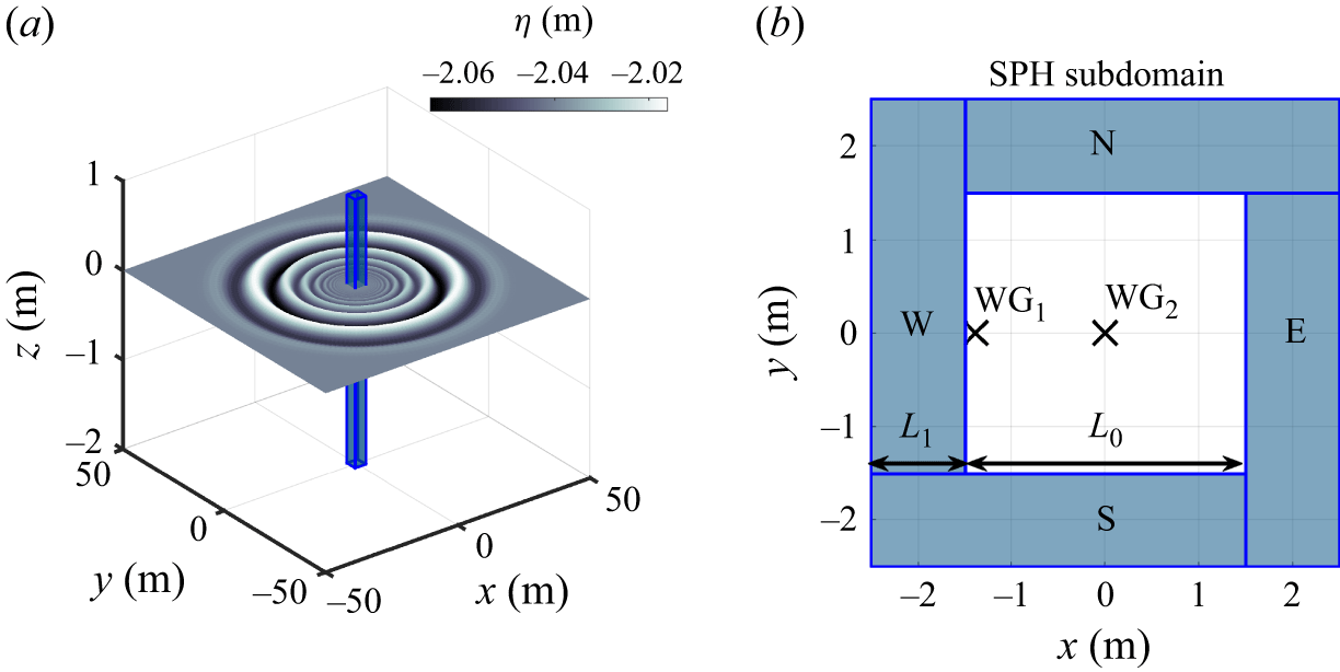
 WG1
 x,y
 −1.384,0
 WG2
 x,y
 0,0

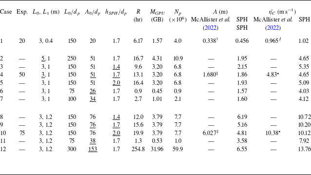
 A
 η˙C
 †
 ‡
 I
 ⋆
 η˙C
 η˙C=2g(A−Acusp)
 Acusp
 L0
 Np
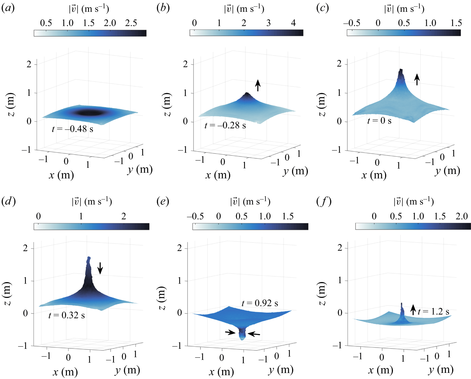


 x=−1.37
 x,y=0

 t=0.2
 t=0.28


 a/g
 y=0
 t=−0.48,−0.44,−0.36

 γ

 γ
 τ
 |a/g|
 t=−0.46
 τ=0

 F(t)
 D(t)
 P(t)
 I(t)
 z
 A0/dp=76
 153

 xz
 y=0
 w
 ωy
 xz
 y=0

 xz
 y=0
 w
 ωy
 xz
 y=0


 y=0
 H(t)
 L(t)


 zt
 zb
 ztp
 zp
 ztp
 A
 zp
 ztp
 ztp
 ztp
 ztp>zp


 WG1
 A0/dp

 A0/dp

 D(t)/dp
 z
 dp
 z
 A0/dp

 y=0

 hSPH/dp
 hSPH/dp=1.4
 hSPH/dp=1.7
 hSPH/dp=2.0
 A0/dp

 Open access

