3.1. Local mapping

Here, we are interested in modeling places with local maps of the environment using 2D LiDAR local features. Instead of modeling a place with features extracted from a single laser reading, our approach locally collects information from multiple scans in order to describe a place with persistent features only. We use FLIRT [Reference Tipaldi and Arras21] operator to extract 2D keypoints from individual scans. This operator combines a curvature-based detector with a beta-grid descriptor. It has shown good repeatability and precision performance in refs. [Reference Tipaldi and Arras21, Reference Tipaldi, Braun and Arras22]. Its multiscale capacity allows to cope with varying laser points density. In addition, this operator is orientation invariant. More details on FLIRT operator are found in refs. [Reference Tipaldi and Arras21, Reference Tipaldi, Braun and Arras22]. Figure 6(a) shows two scans corresponding to sensor poses $i$ and $j$ , represented by the blue and red dots, respectively. FLIRT features are symbolized with blue triangles and red stars, accordingly. For instance, the region of interest $a$ contains two keypoints (one from each scan) and detected with different scales. They have different descriptor values (defined by support points spatial distributions in each neighborhood, delimited by the blue and red circles, respectively). Conversely, region $b$ contains two keypoints with close descriptors at different scales. We qualify such keypoints as stable or persistent. With an appropriate keypoint selection we can obtain a compact and yet consistent representation of the environment. For instance, by keeping one keypoint instance from regions with persistent keypoints only (such as in region $b$ ). Stable keypoint selection strategy is, therefore, key component of our work. It is detailed in the next two subsections.

Figure 6.

Illustration of the mapping process. Two 2D LiDAR scans acquired from two positions $i$ and $j$ corresponding to blue and red colors.

3.1.1. Keypoint stability score

In order to identify regions with high probability of producing similar detector responses, we need to cumulate several scans and count, for each region of interest, the number of keypoint occurrences having similar descriptor values. The submap is, then, built through online selection of stable keypoints among all keypoints from concatenated scans. Scans are registered with ICP [Reference Besl and McKay29] based on libPointMatcher open source library [32]. As stated before, we use FLIRT operator to extract and describe 2D keypoints from individual scans. The FLIRT implementation used in this work is provided by the open source library FLIRTLib [33].

A region of interest or ROI is a region of the environment containing at least one keypoint. In order to count keypoint occurrences in different ROIs we need to define this region in the 2D space. One convenient way to do this is through a regular grid $G$ . Keypoints projected on the grid are grouped into individual cells. In Fig. 6(b), an example of such grid is shown. The grid size adapts with cumulated scan limits in a way that does not affect ROIs’ content. Details of how $G$ is built and updated, as laser scans are concatenated, are given below.

(1) \begin{equation} G(i,j) = \{H, h, m, ns\} \end{equation}

$G(i,j)$ is a cell of $G$ at row $i$ and column $j$ . For the sake of simplicity, we will mention row and column indexes for elements of $G(i,j)$ only when necessary. $h$ and $m$ are, respectively, the laser beam hit and miss counts in this cell, while $ns$ counts the number of laser scans reaching the cell. It is incremented each time a scan produces a value of $h$ greater than zero. $H$ is a list that contains keypoints history for the cell $G(i,j)$ . Its elements are keypoint sets having similar descriptor values, such as

(2) \begin{equation} H = \{H_{0}, H_{1},\cdots,H_{n-1}\} \end{equation}

$H_{k}$ with $k$ in $[0, n-1]$ is a set of keypoints with similar descriptor values, called history cluster. Based on the work of Tipaldi et al. [Reference Tipaldi, Braun and Arras22], descriptors are similar when the symmetric ${\chi }^2$ distance between them is within the value $0.4$ . For every new keypoint falling in $G(i,j)$ , we look for a match with keypoints in every history cluster of $H$ . If a match is found, the keypoint is inserted in the corresponding cluster. Otherwise, a new history cluster is created with the new keypoint.

Keypoint basic stability score $s_{b}(i,j)$ for every ROI delimited by $G(i,j)$ is then easily defined as

(3) \begin{equation} s_{b}(i,j) = \frac{\textrm{occ}}{ns} \end{equation}

$\text{occ}$ corresponds to the occurrence count in the largest history cluster in $H$ , such as

(4) \begin{equation} \textrm{occ} = \vert H_{q} \vert \end{equation}

with $q$ being the index of the largest history cluster in $H$ . In practice, $H$ is sorted by decreasing cluster size. In that case, $q = 0$ . Also, this means that for a new keypoint projected in $G(i,j)$ , the largest history clusters are the first to be considered for a match. In order to use keypoints from areas with high occupancy probability, the stability score in Eq. (3) can be weighted with the density $d$ as follows.

(5) \begin{equation} s(i,j) = d \times s_{b}(i,j) \end{equation}

where $d$ is the occupancy density defined by $d = h/(h+m)$ . In addition, one can set a lower bound $ns_{\textrm{min}}$ for $ns$ (if $ns \lt ns_{\textrm{min}}$ then $ns = ns_{\textrm{min}}$ ). This can be used to impose a minimal scan number reaching a ROI before considering its contribution fully. We use the score defined in Eq. (5) with $ns_{\textrm{min}} = 4$ . The following subsection details the submap construction based on the keypoint stability score exposed here.

3.1.2. Stable keypoints selection for submap construction

Thanks to the stability score above, we can now select stable keypoints to be included in our submap as scans are concatenated. The data structure of a submap $S$ is defined below.

(6) \begin{equation} S = \{P, F\} \end{equation}

where $P = \{p_{0},\cdots, p_{n_{p}-1}\}$ are the $n_{p}$ global poses corresponding to the concatenated scans used during the construction of $S$ . $F$ is the set of stable keypoints expressed in the local frame of $S$ named $p_{\textrm{ref}}$ and which corresponds to the first element of $P$ . The local mapping algorithm is given below.

Algorithm 1 builds a submap $S$ starting at scan index $i_{\textrm{init}}$ from a data set containing $N$ laser scans and their corresponding global poses. Functions $ReadLaserData$ and $GetPose$ respectively output the current local laser reading $\mathcal{L}$ and the corresponding global pose $p$ . Depending whether we use ground truth transforms for scan concatenation or a registration algorithm, $GetPose$ may simply read the provided transforms, or employ scan registration to infer the global pose. $p_{s}$ is the current pose with regard to the submap reference frame $p_{\textrm{ref}}$ . $G$ and $S$ are updated with the functions $UpdateG$ and $UpdateS$ as follows.

• $UpdateG (G, p_{s}, \mathcal{L})$

  • – Transform $\mathcal{L}$ data in the local frame of $S$ thanks to $p_{s}$ such as $\mathcal{L}_{s} = p_{s} \times \mathcal{L}$

  • – Update dimensions of $G$ according to $\mathcal{L}_{s}$

  • – Update $h$ , $m$ , and $ns$ counters in $G$ with $\mathcal{L}_{s}$

  • – Extract FLIRT keypoints from $\mathcal{L}_{s}$ and save them in the current keypoint list $K$

  • – For every keypoint in $K$

    • * Find its corresponding cell in $G$ , $G(i,j)$ and update its keypoint history $H$ as described in Section 3.1.1.

    • * Compute the corresponding stability score $s(i,j)$ according to Eqs. (3)−(5)

• $UpdateS (S, p, G)$

  • – Insert global pose $p$ in the list $P$

  • – For every cell $G(i,j)$ with $H(i,j)\neq \{\}$

    • * If $s(i,j) \geq s_{\textrm{min}}$ select a keypoint from $H_{q}(i,j)$ (for instance, the most recent keypoint) and save it in the stable keypoints list $K_{s}$

  • – Overwrite the list of keypoints $F$ with $K_{s}$

3.1.3. Submap completion criteria

During the mapping process, while exploring the environment, we consider that a robot has finished visiting the current place when overlap ratio $\rho$ between the current and initial submap areas drops below a threshold. There are different ways to estimate this overlap ratio. For instance, it can easily be computed from occupancy grid map as follows.

(7) \begin{equation} \rho = \frac{a_{\textrm{int}}}{a_{\textrm{uni}}} \end{equation}

where $a_{\textrm{int}}$ and $a_{\textrm{uni}}$ are respectively, the intersection and the union areas between initial and current occupancy grids. The current occupancy grid map is available in $G$ . This method requires to keep in memory the initial occupancy grid corresponding to the grid built with the first scan only, during submap construction. For the computation of $a_{\textrm{int}}$ and $a_{\textrm{uni}}$ it is enough to use binary grids. Hence, keeping the initial grid will have negligible memory footprint. In a study not reported in this document, we empirically set the overlap ratio threshold $\rho _{\textrm{min}}$ to $0.75$ . In addition to this criterion, we introduce a submap quality measure that can serve as an additional criterion for submap termination. It is defined in the the following paragraph.

Keypoint spatial distribution: a submap quality measure

As scans are concatenated, the population of stable keypoints in $S$ evolves. Their spatial distribution with regard to the distribution of laser points in the submap is an interesting feature to evaluate the submap quality. In some way, this parameter measures the descriptiveness of the submap. It is defined as follows.

(8) \begin{equation} \delta = \textrm{dist}(h_{lp}, h_{kp}) \end{equation}

where $\text{dist}$ is an histogram distance function, in our case it corresponds to the symmetric ${\chi }^2$ distance. $h_{lp}$ and $h_{kp}$ correspond to the laser points histogram and the keypoints histogram, respectively. They are 2D binary histograms obtained from the occupancy grid map extracted from $G$ . Figure 7(a) shows the occupancy grid map with laser points in white and keypoints surrounded with red circles. We use another grid $D$ to divide space into cells of size $l$ . In our case $l$ is set to $0.5\,\textrm{m}$ , which represents a suitable spatial discretization step for indoor environments. Laser points histogram $h_{lp}$ is a 2D matrix with the same dimensions as $D$ . When a cell $D(i,j)$ contains a laser point, $h_{lp}(i,j)$ takes value $1$ , which corresponds to all non black cells in Fig. 7(b), otherwise it is set to $0$ . The same reasoning is applied to $h_{kp}$ , for which cells take value $1$ for keypoints only, corresponding to the red cells in Fig. 7(b). The histograms are normalized with the respective population in each category of points. Thus, the maximum value for the histogram ditance $\delta$ is $1$ .

Figure 7.

Illustration of spatial distribution quantification for keypoints and laser points.

The submap $S$ is complete if the overlap ratio $\rho$ , defined in Eq. (7) becomes inferior to $\rho _{\textrm{min}} = 0.75$ . Furthermore, the spatial distribution distance defined in Eq. (8) can be used as an additional submap completion criterion, as we will see in Section 5.2.

3.2. Global mapping

We have seen, so far, how to build a local map, corresponding to a place. The global map is a collection of places and is, therefore, represented by a list of submaps with a certain overlapping between successive submaps. The following pseudo-code (Algorithm 2) summarizes the global mapping process that results in the global map $M$ , using $N$ laser scans.

The function $LocalMapping$ calls the local mapping Algorithm 1. It takes as argument the index $i_{\textrm{init}}$ and builds a new submap $S$ starting from scan index $i_{\textrm{init}}$ . When $S$ is complete ( $S \neq \{\}$ ) it is inserted as a new element of the list $M$ . The boolean variable $Success$ is then set to true, and $i_{\textrm{init}}$ is updated such that the next submap starts at the scan positioned after the last scan in $S$ . Therefore, $i_{\textrm{last}}$ corresponds to the size of $P$ , which gives the number of poses (and the number of scans) in $S$ . The global mapping ends when $LocalMapping$ returns an empty submap. When this happens, it means that $LocalMapping$ has reached final scan index $N$ in the data set, without being able to complete the submap $S$ . In practice, this occurs when $i_{\textrm{init}}$ becomes too close to $N$ (or becomes larger than $N$ ), in such a way that there is not enough scans (or no more scans) left to complete a submap.

4.1. Submap matching

A submap consists of a list of stable keypoints. For submap matching we can either match individual keypoints or use a submap signature, for instance in the form of an histogram. In this work, we follow the first approach based on a nearest neighbor pairing. The second approach will thoroughly be studied in another work.

To describe our submap matching algorithm, let us consider two submaps $S_{r}$ and $S_{c}$ . The first is the reference submap belonging to the global map $M$ , while the second is the currently built submap and for which we look for a match in $M$ . Our matching algorithm proceeds as follows.

where $pair$ is a pair formed by keypoint $kp_{c}$ from $F_{c}$ and its matched keypoint $kp_{r}$ from $F_{r}$ . Keypoints $kp_{c}$ and $kp_{r}$ are matched if the distance between their descriptors is below $0.4$ and if none of them was already matched before. The set $pairs$ contains all unique matches between keypoints from $S_{r}$ and keypoints from $S_{c}$ . We remind that coordinates of keypoints in $pairs$ are expressed in their respective submap coordinate systems, corresponding to the first elements of $P_{r}$ and $P_{c}$ . The two submaps are considered a successful match if there is enough unique matches between them. We will see later how we set the threshold $\mu$ .

For the submap $S_{c}$ , there may be more than one match in $M$ . All successfully matched submaps from $M$ are stored in the candidates set $C$ . This set is sorted by increasing average descriptor distance, between matched keypoints in the set $pairs$ . Hence, the first element in $C$ is the best match with $S_{c}$ in terms of average descriptor distance.

4.1.1. Pose estimation

Depending whether we perform global localization or SLAM, the global map $M$ is either complete or in progress. In both cases poses in $P_{r}$ are known and expressed in the global frame. The poses in $P_{c}$ for submap $S_{c}$ are expressed with regard to $P_{c}[0]$ (in the case of global localization) or global but inaccurate (in the case of SLAM). The estimated global pose $\hat{p}$ is obtained using RANSAC [Reference Fischler and Bolles28] which takes as inputs the local keypoints in $F_{r}$ and $F_{c}$ , and returns the rigid transform $\hat{T}^{c}_{r}$ expressing the pose $P_{c}[0]$ with regard to $P_{r}[0]$ ( $X[0]$ symbolizes the first element of the set $X$ ). $\hat{p}$ is given by Eq. (9)

(9) \begin{equation} \hat{p} = P_{r}[0] \times \hat{T}^{c}_{r} \times p_{c} \end{equation}

where $p_{c}$ corresponds to the last element of $P_{c}$ expressed with regard to $P_{c}[0]$ .

We use RANSAC implementation provided in the FLIRT open source library from ref. [33]. The algorithm randomly selects a pair of descriptor based matches and infers a rigid transform relating their 2D coordinates. Applying this transform to bring the two keypoint sets in the same frame, the algorithm counts the number of inliers having an Euclidean distance below an acceptance threshold (set to $0.1\,\textrm{m}$ in our case, based on the works in ref. [Reference Tipaldi, Braun and Arras22]). The random selection is repeated for a number of iterations and the consensus corresponds to the largest inliers set, for which the infered transform $\hat{T}^{c}_{r}$ is returned as output.

4.2. Geometric verification

In the literature, place recognition usualy includes a geometric verification step, to eliminate wrong place matches. Indeed, the appearance of a place may have more than one match in the global map, which do not necessarily correspond to the same location. This is mainly due to visual aliasing and to environments featuring symmetries. This issue is even worsen in the case of 2D LiDAR data, because of its poor nature. The main idea behind geometric verification is to verify the validity of the place matching using geometric criteria, such as the consistency of the rigid transform relating the matched places. In our case, this verification is applied on the first $n_{c}$ elements of the set $C$ defined in Section 4.1. We set $n_{c}$ equal to $500$ in order to consider most of the candidate matches during geometric verification. Our geometric verification, described below, is twofold.

4.2.2. Second geometric verification

In the first verification, a minimal size for RANSAC [Reference Fischler and Bolles28] consensus is imposed. However, this is not enough since we are not sure that all elements of the consensus constitute descriptor based matches. Indeed, they are paired using Euclidean geometric distance only. For the second verification, let us consider the case of a perfect submap match, resulting in a correct loop transform $\hat{T}^{c}_{r}$ . Using this transform to bring the keypoints from both submaps in the same coordinate system, we obtain a keypoint overlap area. Our assumption is that most keypoint matches in this area should be correct matches, not only from a geometric point of view, but also with their descriptors. However, since we are not in an ideal case (the detector and descriptor are not ideal, and the scans are not perfectly aligned), we expect that only a certain proportion $\gamma$ of keypoints in that area has close neighbors that are also matched based on their descriptors. We qualify these points as "doubly” matched keypoints. A pair of keypoints is said doubly matched when the symmetric ${\chi }^2$ distance between their descriptors is within $0.4$ and the geometric distance between their positions does not exceed the threshold $\lambda$ , set in Section 5.2. We define the proportion $\gamma$ in Eq. (10) below.

(10) \begin{equation} \gamma = \frac{2 \times n^{ol}_{dm}}{n^{ol}_{r} + n^{ol}_{c}} \end{equation}

where $n^{ol}_{dm}$ stands for the number of doubly matched keypoints ( $dm$ subscript) in the overlap area ( $ol$ superscript), $n^{ol}_{r}$ and $n^{ol}_{c}$ are, respectively, the number of keypoints from $S_{r}$ and $S_{c}$ in that area. The higher is $\gamma$ the better is the submap match quality. In the ideal case, every keypoint from one submap in the overlap area has a doubly matched keypoint in the other submap, hence $n^{ol}_{dm} = n^{ol}_{r} = n^{ol}_{c}$ , meaning that $\gamma$ would be equal to 1, its maximal value. The submap $S_{r}$ is finally considered a valid match with $S_{c}$ if $\gamma$ is beyond a threshold $\gamma _{\textrm{min}}$ , which value is set in Section 5.2. The overlapping area is approximated by the intersection of the bounding boxes delimited by keypoint coordinates from each submap.

5.1. Mapping parameter setting

We assess the mapping algorithm for different values of $l_{g}$ and $s_{\textrm{min}}$ . In order to find optimal values for these parameters, we define the following quality criteria that the map should meet.

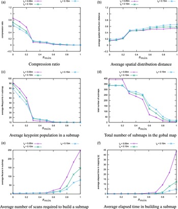
• Compression ratio − The compression ratio is the ratio between the number of stable keypoints in the global map and the total number of keypoints from all scans. The lower it is, the higher is map data reduction.

• Average number of scans in a submap − This criterion measures an average of the number of scans in a submap, from all the submaps in the global map. This gives a sense of how many scans are required to map a place.

• Average number of keypoints in a submap, and

• Average spatial distribution distance − The spatial distribution distance measures the difference between the spatial distribution of keypoints and that of all laser points in a submap, as defined in Eq. (8). The two latter quantities inform us on keypoint population in the submaps. A submap must contain enough keypoints to be distinguishable among other places. On the other hand, these keypoints should be well distributed in space. The lower is the spatial distribution distance the better is the submap description of a place.

• Total number of submaps in the global map

• Average elapsed time in building a submap

The six criteria above are evaluated while varying $s_{\textrm{min}}$ from $0$ to $1$ with a step of $0.1$ . This is repeated for three grid cell size values $l_{g} = 0.05\,\textrm{m}$ , $l_{g} = 0.1\,\textrm{m}$ , and $l_{g} = 0.15\,\textrm{m}$ .

We want to maximize keypoint population in a submap while minimizing the compression ratio, the spatial distribution distance, the number of scans in a submap and the elapsed time in building a submap. Observing Fig. 8, the values $s_{\textrm{min}} = 0.3$ and $l_{g} = 0.1$ represent a good tradeoff to reach this objective. Table II summarizes the results obtained for all data sets using these parameter values. The compression ratio is in the worst case equal to $0.15$ , corresponding to a reduction of $85\%$ in map data, which is significant. This reduction reaches $88\%$ in the best case. Less than six scans, in average, are needed to map a place. Submap keypoint population is beyond $14$ keypoints with spatial distribution distance not exceeding $0.54$ . This value is acceptable, considering that the maximal value for this distance is $1$ . Submaps are built with a rate of $9.2\,\textrm{Hz}$ in the worst case and $17.5\,\textrm{Hz}$ in the best case.

Figure 8.

Evolution of mapping quality criteria as a function of parameters $s_{\textrm{min}}$ and $l_{g}$ .

Table II.

Mapping criteria results for optimal parameter values, and for the three corrected maps. Compress. corresponds to the average compression ratio, $\#$ Scans is the average number of scans required to build a submap, $\#$ Keypoints is the average number of stable keypoints in a submap, Distrib. is the average spatial distribution distance, and $\#$ Submaps is the number of submaps in the global map. Time is the average spent time in submap construction.

5.2. Place recognition parameter setting

There are three main parameters in the place recognition process. The first is the minimal number of unique keypoint matches, $\mu$ in the submap matching step described in Section 4.1. The second parameter is the minimal ratio of doubly matched pairs $\gamma _{\textrm{min}}$ in the second geometric verification described in Section 4.2.2. The third parameter is the maximal geometric distance $\lambda$ separating a pair of doubly matched keypoints, in the second geometric verification as well. In order to set optimal values for these parameters, we measure performance of our algorithm in terms of precision and recall, in the context of global localization. A global map $M$ is built beforehand using the corrected data. Then, using these data a submap $S_{c}$ is started from an arbitrary global position, unknown to $S_{c}$ . In this case, $P_{c}[0]$ is the identity matrix. Finally, the place recognition algorithm provides an estimate of the global pose $\hat{p}$ by finding for $S_{c}$ the matching submap $S_{r}$ in the global map $M$ , as described in Section 4.1.1. In order to avoid automatching with an identical submap from $M$ , if a matched submap $S_{r}$ is built with the exact same scans as $S_{c}$ , the match is ignored. A similar evaluation process is used in the literature, such as in refs. [Reference Tipaldi, Spinello and Burgard20–Reference Tipaldi, Braun and Arras22, Reference Deray, Solà and Cetto25].

The algorithm is assessed for $4$ values of $\mu$ and $11$ values of $\gamma _{\textrm{min}}$ , respectively $\{5, 10, 15, 20\}$ , and $[0, 1]$ with a step of $0.1$ . This experiment is run for $\lambda = 0.05\,\textrm{m}$ . In a later stage, the obtained optimal parameters are used for performance evaluation with $\lambda = 0.1\,\textrm{m}$ . In addition to these parameters, we impose a minimal number of keypoints in a submap to be consistent with the minimal required size for RANSAC’s consensus (set to $9$ ). Therefore, we decide to set $10$ as a minimal size for the submap, in terms of keypoint population. On the other hand, based on previous analysis on the mapping process given in Section 5.1, in addition to the drop in overlap ratio, we impose another criterion for submap completion that is the spatial distribution distance $\delta$ , which should not exceed $0.5$ , in order to guarantee an optimal spatial distribution of keypoints. We remind that, based on the results obtained in Section 5.1, the average submap’s keypoint population is beyond $10$ and the average spatial distribution is around $0.5$ . This evaluation is performed using the data set $FR079$ , then the obtained parameters are used for $FR101$ and $Intel$ data sets.

Figure 9.

Global localization − Precision and recall for $FR079$ , $\lambda = 0.05\,\textrm{m}$ .

The pseudo code for global localization evaluation, used here, is given in Algorithm 4. The function $PlaceRecognition$ combines submap matching and geometric verification. The function $Evaluation$ computes precision and recall by comparing $\hat{p}$ with $p$ , respectively the estimated pose given by Eq. (9), and ground truth pose. The pose estimate $\hat{p}$ is considered correct if the translation and rotation errors, with regard to $p$ , are within $0.5\,\textrm{m}$ and $10^{\circ }$ , respectively [Reference Tipaldi, Spinello and Burgard20−Reference Tipaldi, Braun and Arras22, Reference Deray, Solà and Cetto25, Reference rizzini, Galasso and Caselli26]. The global localization is performed $n_{\textrm{pos}}$ times corresponding to equally spaced starting positions for the current submap $S_{c}$ . In our case, $n_{\textrm{pos}} = 500$ . The average precision and recall is computed over $n_{\textrm{pos}}$ , for all combinations of place recognition algorithm parameters. Precision and recall are defined as

(11) \begin{equation} \textrm{precision} = \frac{n_{\textrm{cor}}}{n_{\textrm{acc}}} \end{equation}

(12) \begin{equation} \textrm{recall} = \frac{n_{\textrm{cor}}}{n_{\textrm{pos}}} \end{equation}

$n_{\textrm{cor}}$ and $n_{\textrm{acc}}$ correspond respectively, to the number of truly correct localizations (true positives), and the number of localizations considered correct (accepted) by the algorithm (true positives + false positives).

Figure 9 shows precision and recall obtained for $FR079$ data set with $\lambda = 0.05\,\textrm{m}$ . In terms of precision, the results obtained with the four values of $\mu$ are similar and reach the maximum precision value $1$ , although one can notice that the precision is better for larger values of $\mu$ and $\gamma _{\textrm{min}}$ together. The impact of $\mu$ and $\gamma _{\textrm{min}}$ is more visible when observing recall results. For $\mu = 10$ and $\gamma _{\textrm{min}} = 0.4$ we obtain a recall and precision tradeoff that maximizes precision. Table III summarizes results obtained applying these values to the other corrected data sets. For all three data sets, we obtain a good recall level at precision of $1$ , which is particularly recommended for loop closure detection in SLAM.

Table III.

Global localization results for corrected data, obtained with $\mu = 10$ , $\gamma _{\textrm{min}} = 0.4$ , and $\lambda = 0.05\,\textrm{m}$ .

Table IV gives the results obtained for $\lambda = 0.1\,\textrm{m}$ . Comparing with the results in Table III, increasing this parameter improves recall results while keeping the precision at a high level. The last two columns in Tables III and IV inform us on the average number of scans required to perform a correct localization and the corresponding spent time.

Table IV.

Global localization results for corrected data, obtained with $\mu = 10$ , $\gamma _{\textrm{min}} = 0.4$ , and $\lambda = 0.1\,\textrm{m}$ .

5.3. Summary of parameter setting

We summarize, here, the results obtained for the five parameters in our approach. Table V gives parameter values for the mapping and place recognition algorithms. These parameters are imposed by mapping quality criteria and place recognition objectives. For the mapping stage, we have defined in Section 5.1 six criteria among which the most important, in our case, is the map data compression ratio. Place recognition parameter setting relies on precision and recall optimization in the context of global localization. We made the choice of maximizing precision while keeping an acceptable recall level.

Table V.

Optimal parameters.

6.1. Mapping evaluation

We apply the mapping algorithm on the raw data sets $FR079\_r$ , $FR101\_r$ , and $Intel\_r$ , using parameter values obtained from previous section, that is, $s_{\textrm{min}} = 0.3$ and $l_{g} = 0.1$ . Scans are registered with ICP. The results are given in Table VI. Comparing with the results in Table II, we first notice an increase in the number of scans required to build a submap. This is mainly due to the density of raw data in terms of scans, which also explains the increase in the number of submaps in the global map. As a consequence, the average keypoint population is higher, with a better spatial distributions ( $\delta = 0.4$ for the worst case). The compression ratio remains at a very low level, corresponding to $85\%$ of map data reduction in the case of $Intel\_r$ , and $88\%$ for $FR079\_r$ . Execution time shows that we can build submaps, in the worst case at a rate of $2.17\,\textrm{Hz}$ , and $3.85\,\textrm{Hz}$ for the best case. The mapping process takes more time here, due to scan registration with ICP and to a larger number of scans in the submaps.

Table VI.

Mapping criteria results for optimal parameter values and for the three raw data sets.

6.2. Place recognition evaluation

Place recognition is evaluated using raw data for two applications. The first is global localization and the second is loop closure detection in the context of SLAM.

6.2.1. Global localization

Similarly to Section 5.2, a global map $M$ is built using the corrected data, then starting from an unknown position, a submap $S_{c}$ is built in order to perform global localization using our place recognition approach. The main difference with the experiment in Section 5.2 is that $S_{c}$ is built using raw data. Scans in $S_{c}$ are registered with ICP. Not all raw poses have a corresponding ground truth pose among corrected data. In order to measure precisison and recall, we need a mapping that relates each ground truth pose with its corresponding raw pose. Submap $S_{c}$ starts at arbitrary positions among raw poses for which a ground truth value exists. ICP is initialized with the odometry provided in raw data. We run the global localization algorithm using parameters from previous section, that is, $\mu = 10$ , $\gamma _{\textrm{min}} = 0.4$ , and $\lambda = 0.05$ . An additional evaluation is performed for $\lambda = 0.1$ . Mapping algorithm parameters are those given in Table V.

Comparing the results in Tables VII and VIII with the results in Tables III and IV, we notice that the precision remains very high (almost $1$ ) in all cases but the recall level decreased. This is particularly true for $FR101\_r$ data set, when using a value of $0.05\,\textrm{m}$ for $\lambda$ . It takes more scans, in the raw data case, to correctly localize the robot, which is expected since in this case the displacements are smaller. Compared to the case of corrected data, localization takes more time due to higher keypoint population in raw data submaps, and larger global maps in term of submap population.

Table VII.

Global localization results for raw data, obtained with $\mu = 10$ , $\gamma _{\textrm{min}} = 0.4$ , and $\lambda = 0.05\,\textrm{m}$ .

Table VIII.

Global localization results for raw data, obtained with $\mu = 10$ , $\gamma _{\textrm{min}} = 0.4$ , and $\lambda = 0.1\,\textrm{m}$ .

Comparing the results in Tables VII and VIII, the same conclusion as in Section 5.2 can be drawn regarding how $\lambda$ impacts recall results. For $FR101\_r$ with $\lambda = 0.1\,\textrm{m}$ , recall has significantly improved (more than doubled) in comparison with the recall obtained for $\lambda = 0.05\,\textrm{m}$ . Considering the last column in Tables VI−VIII, we can map a place and correctly localize the robot at a rate of $2.55\,\textrm{Hz}$ in the best case, and $1.98\,\textrm{Hz}$ in the worst case.

6.2.2. Loop closure

Here, we are interested in evaluating the possibility of integrating our place recognition approach in a SLAM framework, for loop closure detection using parameters in Table V. To this end, we employ a SLAM implementation provided in the GTSAM open source library [34]. It is a pose-graph SLAM variant based on factor graphs. For our evaluation we use this tool with its defaults parameters, except for covariances that we have set empirically. Furthermore, only submap poses are included in the graph and no features are used in the graph optimization process. Therefore, we do not expect to build precise maps. However, with this setup, we aim at evaluating our approach by examining the produced trajectories using raw data. We remind that for these data, not all poses have a corresponding ground truth in the corrected data. There is no guaranty that a submap built with raw data contains a pose for which the ground truth is known. Therefore, in order to decide wether a loop is correct, we rely on overlap rate between matched submaps. The overlap rate is also used in ref. [Reference Zlot and Bosse17] to decide for correct submap matches. Obviously, this assumes a limited drift due to odometry and scan registration errors. Considering this assumption, we reject all matches of submap pairs with no overlap, and we impose a minimal overlap ratio of $0.01$ between matched submaps.

Loop closure and mapping analysis

Figure 10(a,c,e) depict the trajectories obtained with SLAM using our place recognition approach for loop closure, respectively for $FR079\_r$ , $FR101\_r$ , and $Intel\_r$ data sets. The trajectory drawn with red dots correspond to estimated submap poses. As a reference, for visual comparison, we display the trajectory produced by the corrected data with green dots.

Figure 10.

Left: SLAM trajectory in red versus ground truth trajectory in green. White discs represent positions of loop detections used in the pose graph, large green disc is the initial position, small green disc is the first loop detection position. Right: matched submap overlap histograms. Results for $FR079\_r$ , $FR101\_r$ , and $Intel\_r$ are given in each row, respectively.

For $FR079\_r$ and $FR101\_r$ , the trajectory obtained with SLAM is consistent with the correct trajectory. As expected, due to pose drift and to possible false loop closures, it does not exactly match the ground truth trajectory. In the case of $Intel\_r$ , the trajectory is globally consistent. However, because of an erroneous loop closure, we notice an inconsistency at the bottom left side of Fig. 10(e). We remind that our pose-graph considers poses only, and does not include features, which impacts the graph SLAM performance. In addition, among all detected loops, only a small subset of loops is used in the graph optimization. Since we update the graph each time a new loop is detected in order to update the global map $M$ , we do not use all the detected loops, as these two update operations are time consuming.

Figure 10(b,d,f) show histograms of overlap rate between all matched submaps for each data set. The histogram has five bins corresponding to overlap rates in the following intervals $[0, 10[$ , $[10, 20[$ , $[20, 30[$ , $[30, 40[$ , and $[40, 100]$ . For all data sets, most matched submaps overlap with a rate larger or equal to $40\%$ . For $FR079\_r$ , a total of $82$ loops are detected while $184$ are detected in $FR101\_r$ and $572$ in $Intel\_r$ (among all these loops, only a limited number of $13$ , $12$ , and $47$ loops are used in the pose graph, respectively for $FR079\_r$ , $FR101\_r$ , and $Intel\_r$ ). In a pessimistic evaluation, if we consider that $30\%$ overlap is required to decide for a correct match, then the precision values are respectively $73/82 = 0.89$ , $169/184 = 0.92$ , and $503/572 = 0.88$ for the three maps. In a more tolerent evaluation, if $10\%$ overlap rate is enough to decide for a correct loop closure, then the precision values raise to $82/82 = 1$ , $184/184 = 1$ , and $569/572 = 0.99$ , respectively. In both evaluations, $Intel\_r$ gives the lowest precision value.

Table IX gives map characteristics for the three data sets. Compared to Table VI, all maps feature better map data reduction (up to $92\%$ for $FR079$ ) with less submaps in the global map. This is due to map correction with SLAM, which also explains the decrease in submap keypoints population. We notice also a slight improvement in keypoints spatial distribution.

Table IX.

Mapping criteria results for optimal parameters, and for the three corrected maps with SLAM using raw data.

Trajectory error analysis

As an additional evaluation, we measure RPE (relative position error) and ATE (absolute trajectory error) for all trajectories. The RPE gives a sense of the drift for different time intervals between two poses of the robot. It is defined in Eq. (13)

(13) \begin{equation} E_{i} \;:\!=\; (Q^{-1}_{i}Q_{i+\Delta })^{-1}(P^{-1}_{i}P_{i+\Delta }) \end{equation}

with $Q_{i}$ and $P_{i}$ being respectively ground truth and estimated poses at time index $i$ . $\Delta$ is a fixed time interval. For a trajectory with $n$ poses, we obtain $m = (n-\Delta )$ RPE values along the trajectory [36]. In the literature, authors often evaluate the RMSE (root mean square error) obtained for different values of $\Delta$ and define in Eq. (14). Note that in our case, $\Delta$ corresponds to data index interval.

(14) \begin{equation} \textrm{RMSE}(E_{1:n}, \Delta ) \;:\!=\; \left(\frac{1}{m} \sum _{i=1}^{m}\left( \| \textrm{Trans}(E_{i}) \|^2 \right)\right)^{\frac{1}{2}} \end{equation}

The operator $\text{Trans}$ returns the translation component of error matrix $E_{i}$ . One can also obtain the RMSE of the rotation RPE by infering the rotation from $E_{i}$ .

The ATE measures absolute translation and rotation errors between the estimated poses and the corresponding ground truth poses. It is defined as follows.

(15) \begin{equation} F_{i} \;:\!=\; Q^{-1}_{i} A P_{i} \end{equation}

where $A$ is the transform that maps the estimated trajectory on the ground truth trajectory [36]. Figure 11 shows RMSE of RPE results for each data set. For $FR079\_r$ and $FR101\_r$ translation and rotation errors do not exceed $1.3\,\textrm{m}$ and $9^{\circ }$ , respectively. In comparison, the case of $Intel\_r$ data set exhibits higher error levels, especially for the rotation. Figure 12 shows ATE errors for each data set, as a function of path length. Similar conclusions can be drawn for the quality of trajectories that is better for $FR079\_r$ and $FR101\_r$ , compared to $Intel\_r$ . It is interesting to notice the peaks in ATE errors for $Intel\_r$ , especially between path lengths $150$ and $200\,\textrm{m}$ . This corresponds to erroneous loops which consequence on the trajectory can be observed on Fig. 10(e) (bottom left side). This explains the high RPE errors for this map. This also shows that the algorithm manages to find new correct loops that help to rectify the trajectory.

Figure 11.

RMSE of RPE as a function of $\Delta$ . Left: translation error. Right: rotation error. Results for $FR079\_r$ , $FR101\_r$ , and $Intel\_r$ are given in each row, respectively.

Figure 12.

ATE as a function of path length. Left: translation error. Right: rotation error. Results for $FR079\_r$ , $FR101\_r$ , and $Intel\_r$ are given in each row, respectively.

6.3. Discussions with regard to state-of-the-art

In the previous subsections, we have shown that we can achieve a high level of map data reduction while maintaining good performance in terms of precision and recall. In the literature, most local feature based methods in this field encode a place with a single scan, such as in refs. [Reference Tipaldi, Spinello and Burgard20−Reference Deray, Solà and Cetto25]. In that case, the global map contains all features from all scans. As a consequence, the map data size inevitably keeps growing with the number of laser readings. For larger environments, it is of great interest to reduce the map data. The work of Bosse and Zlot [Reference Bosse and Zlot16, Reference Zlot and Bosse17] is the most similar to ours as they model places with local maps or submaps. Submaps contain keypoints selected from concatenated laser scans. The authors provide no significant results on map data reduction. They terminate a submap when the state vector (used in local mapping through a Kalman filter) reaches a certain size. In our work, a keypoint stability score allows to detect areas with persistent features from concatenated scans, and achieve considerable map data reduction. We use the state-of-the-art operator FLIRT, which has shown interesting performance in refs. [Reference Tipaldi and Arras21, Reference Tipaldi, Braun and Arras22]. Regarding submap termination, we introduce a submap quality measure based on the spatial distribution of keypoints. This metric together with the overlap rate drop between the current and initial submap areas, serve as criteria for submap completion. Instead of a rigid criterion, our solution is adaptive. It allows to set a minimal overlap between consecutive submaps, and insures that a place is well described before starting a new submap.

Among prominent works on local feature based place recognition using 2D LiDAR data, is that of Tipaldi et al. [Reference Tipaldi, Spinello and Burgard20−Reference Tipaldi, Braun and Arras22]. The authors introduced the FLIRT operator used in our work. They measure two metrics for performance evaluation, namely $P_{GL}$ and $P_{CL}$ . The first is the probability of correct global localization, and it corresponds to precision at maximal recall. The second metric is the probability of loop closure given by recall value at $0.95$ precision. As stated before, the authors encode a place with features from a single scan and no map data reduction is considered (the global map contains all features from every scan). We have evaluated $P_{GL}$ and $P_{CL}$ for data sets $FR079$ and $Intel$ , since these data sets are also used in ref. [Reference Tipaldi, Braun and Arras22]. This evaluation corresponds to the global localization performed in Section 6.2.1. Table X summarizes the results obtained for our approach in comparison with Tipaldi’s residual based approach from ref. [Reference Tipaldi, Braun and Arras22]. We remind that for our evaluation we compare a submap built using raw data (scans registered with ICP) with a global map built from corrected data, whereas Tipaldi’s evaluation compares a scan from the corrected data with the remaining scans from the same corrected data. Despite this condition, the results show that even with a considerable map compression rate ( $88 \%$ for $FR079$ and $85\%$ $Intel$ data sets, respectively) our approach maintains high loop closure and global localization performance. This conclusion is also valid when comparing to the work of Himstedt et al. [Reference Himstedt and Maehle23, Reference Himstedt, Frost, Hellbach, Bohme and Maehle24] on GLARE features and GSR signature. The authors obtain good recall and precision levels but require complex signature calculations and do not consider map data reduction the way it is done here. Finally, approaches such as GFP [Reference Tipaldi, Spinello and Burgard20] and in ref. [Reference Deray, Solà and Cetto25] encode scans with words similarly to bag of words, and therefore require training data sets to generate vocabularies, which is not the case of our approach.

Table X.

Performance comparison with Tipaldi et al. approach [Reference Tipaldi, Braun and Arras22]. Data reduc. stands for map data reduction rate. Ours-X-Y is our approach where $\mu = X$ and $\lambda = Y$ . TIP-FLIRT is Tipaldi’s approach. For easy comparison, TIP-FLIRT results and the best values obtained with our approach are shown in boldface.