1. Introduction
Active flow control of the interaction between deformable structures and surrounding flows, known as fluid–structure interaction (FSI), plays a critical role across various fields, including aerospace, biology, marine and biomedical engineering (Dowell & Hall Reference Dowell and Hall2001; Hou, Wang & Layton Reference Hou, Wang and Layton2012). Among various FSI problems, the active control of flexible flaps placed in bluff body wakes is of particular interest, as it serves as a representative physical model for a range of natural and bio-inspired systems such as robotic fish locomotion (Liao Reference Liao2007; Chung et al. Reference Chung, Cao, Philen, Beran and Wang2018; Wang & Wang Reference Wang and Wang2021). However, such control presents significant challenges due to strong nonlinearities and complex coupling mechanisms. These challenges arise from nonlinear fluid phenomena, including surface vorticity generation and vortex shedding at trailing edges, as well as structural effects, including inertia, bending stiffness and flow-induced tension variations (Connell & Yue Reference Connell and Yue2007). Although reinforcement learning (RL) has shown promise in FSI control by training agents via interaction with full-order FSI simulations, its practical deployment remains limited by the high computational costs of such training (Vignon, Rabault & Vinuesa Reference Vignon, Rabault and Vinuesa2023; Jia & Xu Reference Jia and Xu2025). To overcome this computational barrier and enable the rapid development of an efficient control strategy for an FSI system, this paper develops a predictive control framework based on a Koopman reduced-order model (ROM). We demonstrate our approach on the canonical system of a flexible plate attached to a fixed cylinder in an open flow, with the goal of controlling its flapping dynamics.
This type of FSI system exhibits complex instabilities and bifurcation phenomena, and understanding these dynamics is a prerequisite for implementing effective control. Lee & You (Reference Lee and You2013) investigated the instability of a thin filament (
 $H^* = 0.06D^*$
, where
 $D^*$
is the diameter of the cylinder) at a Reynolds number of
 ${\textit{Re}} = 100$
, finding that the filament’s flapping characteristics were directly dependent on its length
 $L^*$
. Wu et al. (Reference Wu, Qiu, Shu and Zhao2014) explored the passive control of vortex shedding at
 ${\textit{Re}} = 150$
using a thin filament, concluding that by appropriately tuning the filament’s flexibility, the lift force fluctuations and vortex shedding from the cylinder could be effectively suppressed. Pfister & Marquet (Reference Pfister and Marquet2020) studied a filament with
 $(H^*,L^*)=(0.06D^*,2D^*)$
at
 ${\textit{Re}}=80$
, identifying four distinct oscillatory states by varying the Young’s modulus. Furquan & Mittal (Reference Furquan and Mittal2021) studied the flapping of a filament of negligible thickness at
 ${\textit{Re}}=150$
, identifying multiple lock-in branches corresponding to the four structural modes and revealing hysteretic transitions between them. Duan & Wang (Reference Duan and Wang2024) presented an experimental investigation by varying filament length and bending rigidity with
 $H^* = 0.005D^*$
, they identified three distinct response regimes. While these studies model the structure as a one-dimensional filament of negligible thickness, these works clearly show that parameters like length and stiffness directly influence the type of bifurcation and flapping. In contrast, Sahu, Furquan & Mittal (Reference Sahu, Furquan and Mittal2019) extended the Turek and Hron benchmark problem (Turek & Hron Reference Turek and Hron2006) to an open flow and retained the plate’s geometry
 $(H^*,L^*)=(0.2D^*,3.5D^*)$
in a fully coupled FSI simulation at
 ${\textit{Re}}=150$
, discovering different solution branches as the Young’s modulus was varied. However, as noted by Lee & You (Reference Lee and You2013), length plays a crucial role in the instability of the plate and, for this particular thickness, other lengths have not yet been investigated. Specifically, a plate of length
 $L^*=2D^*$
is comparable to the characteristic vortex formation length in the cylinder’s wake, suggesting the potential for strong fluid–structure lock-in and novel resonant states. Moreover, an aspect ratio (
 $L^*/H^*$
) of 10 accentuates the two-dimensional plate-like characteristics over the one-dimensional filament-like behaviour of slender filaments, which could fundamentally alter the primary modes of instability. Therefore, our study focuses on the
 $(H^*,L^*)=(0.2D^*,2D^*)$
configuration to investigate its instability and bifurcation phenomena.
To actively control these FSI dynamics, full-order model (FOM)-based control strategies have been proposed. Failer & Richter (Reference Failer and Richter2021) developed an optimal control algorithm that combines the Broyden–Fletcher-Goldfarh-Shanno (BFGS) optimisation method with a specialised multigrid solver for FSI problems. By fully solving the forward and adjoint equations in each iteration, their method computes the gradient to update the control action. Wang et al. (Reference Wang, Jimack, Walkley, Yang and Thompson2021) proposed an adjoint-based algorithm to control the FSI system by optimising a distributed body force applied within the solid domain. A gradient descent method is employed with the step size efficiently determined by the stabilised Barzilai–Borwein method. Subsequently, they applied this method to control the flapping of a flexible plate in the benchmark FSI problem (Turek & Hron Reference Turek and Hron2006), but it did not completely suppress the oscillations, only achieving a 50 % reduction in amplitude (Wang Reference Wang2022). They all use displacement data from the entire structure as their sensing input, without optimising the probe placement based on practical requirements. Moreover, in addition to modelling difficulties, these FOM-based FSI control strategies suffer from high computational costs, which prevents them from meeting the demands of real-time control applications. A more computationally efficient solution is to construct ROMs that preserve the essential system dynamics while enabling efficient controller design and deployment on the original high-fidelity system. Several reduced-order modelling approaches have been successfully applied for the active control of FSI problems, with most efforts focusing on rigid structures. Specifically, Yao & Jaiman (Reference Yao and Jaiman2017) designed a linear quadratic regulator controller based on an eigensystem realisation algorithm-derived ROM to control vortex-induced vibration (VIV) at
 ${\textit{Re}} = 60$
. Luo, Gao & Zhang (Reference Luo, Gao and Zhang2022) developed an autoregressive with external input methods-based ROM and suppressed VIV by actively controlling a tuned mass damper at
 ${\textit{Re}} = 60$
. Jiang & Cao (Reference Jiang and Cao2024) developed a balanced proper orthogonal decomposition-based ROM for VIV of a cylinder at
 ${\textit{Re}} = 100$
, and used it to design a feedback controller that remained robust over a range of Reynolds numbers. However, most existing methods rely on linearised FSI models, which are readily available for rigid-body motion but difficult to obtain in systems involving flexible structures, where strong nonlinearities and high-dimensional control inputs significantly complicate the modelling and control process. Furthermore, these methods often implicitly assume the availability of full-state measurements for model projection, a requirement that is impractical for most real-world applications.
To overcome these challenges, we advocate for modernising control strategies in FSI and, to this end, propose a Koopman operator-based reduced-order modelling framework for feedback control of such systems. The Koopman operator provides a linear representation of nonlinear dynamical systems by projecting them onto an infinite-dimensional space of observables, enabling the decomposition of high-dimensional spatio-temporal fields into linear combinations of coherent modes ranked by frequency and growth rate (Rowley et al. Reference Rowley, Mezić, Bagheri, Schlatter and Henningson2009). Koopman-based methods have been applied to the analysis of nonlinear FSI dynamics (Güner et al. Reference Güner, Thomas, Dimitriadis and Terrapon2019; Li et al. Reference Li, Kemp, Jaiman and Khoo2021; Rodríguez-López et al. Reference Rodríguez-López, Carter and Ganapathisubramani2021). In these studies, dynamic mode decomposition (DMD) was primarily used to identify main coherent structures, as DMD accuracy is limited by the assumption that the Koopman-invariant subspace lies within the space spanned by the state (Williams, Kevrekidis & Rowley Reference Williams, Kevrekidis and Rowley2015). To discover more accurate and informative Koopman-invariant subspaces, Jovanović et al. (Reference Jovanović, Schmid and Nichols2014) developed sparsity-promoting DMD (spDMD), recasting mode selection in DMD as an optimisation problem with an
 $\ell _1$
penalty. Williams et al. (Reference Williams, Kevrekidis and Rowley2015, Reference Williams, Rowley and Kevrekidis2016) introduced extended and kernel DMD (EDMD/KDMD) that enable projection onto a broader class of nonlinear observable spaces, resulting in more interpretable Koopman spectra and improved accuracy. Brunton et al. (Reference Brunton, Brunton, Proctor and Kutz2016a
) then presented an iterative approach that augments the EDMD dictionary until reaching subspace convergence criteria to further improve accuracy. Despite these advances, a major limitation of EDMD/KDMD is spectral pollution, where spurious modes degrade the model accuracy. To address this issue, Colbrook, Ayton & Szőke (Reference Colbrook, Ayton and Szőke2023) proposed residual DMD (ResDMD), which computes residuals that rigorously identify and eliminate spurious modes. This method not only enhances accuracy but also enables more efficient data compression through residual-based mode ordering. Moreover, ResDMD integrates seamlessly with existing DMD techniques without requiring additional data or introducing computational overhead. More methodological developments in the DMD family can be found in Otto & Rowley (Reference Otto and Rowley2019) and Pan, Arnold-Medabalimi & Duraisamy (Reference Pan, Arnold-Medabalimi and Duraisamy2021). Despite these advances, to address the aforementioned limitation of impractical full-state sensing, the Koopman method struggles to accurately predict the system’s nonlinear behaviour when measurements are sparse. Therefore, employing time-delay embedding to augment the state space by leveraging temporal information to compensate for the lack of spatial data is a crucial step for constructing a high-precision Koopman predictive model (Kamb et al. Reference Kamb, Kaiser, Brunton and Kutz2020; Yuan et al. Reference Yuan, Zhou, Zhou, Wen and Liu2021; Jiang et al. Reference Jiang, Pfister, Huang and Cao2025a
). However, these current methods are primarily designed for autonomous systems and do not account for external inputs, which limit their applicability to control tasks where input-response relationships are essential.
To extend these methods from autonomous systems to systems with external actuation, Proctor, Brunton & Kutz (Reference Proctor, Brunton and Kutz2016) proposed the DMD with control (DMDc) algorithm, which extends DMD to systems with external actuation by simultaneously identifying both the underlying dynamics matrix
 $A$
and the control input matrix
 $B$
from snapshot data. Brunton et al. (Reference Brunton, Proctor and Kutz2016b
) proposed sparse identification of nonlinear dynamics with control (SINDYc), which discovers sparse nonlinear dynamics models by identifying a few active terms from a library of candidate functions that best represent the system’s behaviour under control inputs. Korda & Mezić (Reference Korda and Mezić2018) further developed extended DMDc (EDMDc), which leverages Koopman operator theory to transform nonlinear systems into higher-dimensional spaces where they behave approximately linearly. Zhang et al. (Reference Zhang, Rowley, Deem and Cattafesta2019) introduced online DMD, which recursively updates a low-dimensional linear model of complex dynamics as new data becomes available, enabling real-time system identification. However, since inputs nonlinearly influence the Koopman operator and its eigenfunctions, numerous nonlinear functions of the inputs must be included in addition to state variables in all the above methods. This necessitates collecting substantial data to cover a sufficiently broad dynamic range. To address this issue, Peitz & Klus (Reference Peitz and Klus2019) proposed an alternative approach where the control system is replaced by a set of autonomous systems with constant inputs. Through this method, the optimal control problem is transformed into a switching problem between linear systems in a nonlinear feature space. If sufficient nonlinear features are employed, the original objective can be approximated arbitrarily well. Peitz & Klus (Reference Peitz and Klus2020) further introduced a relaxation technique to reduce computational cost and achieved feedback control of the one-dimensional Burgers equation and two-dimensional Navier–Stokes equations. However, the original implementations relied on standard DMD/EDMD, which can produce spurious modes that significantly degrade the predictive accuracy of the models, leading to suboptimal or even unstable control performance when the framework makes decisions based on faulty predictions. To overcome this critical limitation, our work incorporates a key element of a robust modelling strategy: we develop high-accuracy Koopman-based ROMs using KDMD with time-delay embedding and employ ResDMD to rigorously identify and eliminate spurious modes. By doing so, we significantly enhance the fidelity of the underlying models and propose a new control framework designed for FSI systems with flexible structures.
The predictive nature of these high-fidelity Koopman-based ROMs makes them particularly well suited for the model predictive control (MPC) framework (Lee Reference Lee2011), a receding-horizon control scheme that relies on short-term forecasting to compute optimal control actions. Arbabi, Korda & Mezić (Reference Arbabi, Korda and Mezić2018) proposed a fully data-driven, model-free nonlinear partial differential equation closed-loop feedback control method based on MPC coupled with EDMDc, successfully applying it to boundary control of fluid flow in two-dimensional cavity periodic Burgers and Navier–Stokes equations. Fonzi, Brunton & Fasel (Reference Fonzi, Brunton and Fasel2020) extended the DMDc algorithm in two ways and combined it with MPC algorithms for controlling flexible aeroelastic systems. They developed an interpolation scheme to smoothly connect multiple linear DMDc models developed under different operating conditions. Wang & Shoele (Reference Wang and Shoele2024) presented an active flow control framework based on MPC along with a DMDc ROM, utilising wing deformation to regulate wing-surface flow-induced flutter. Marra, Meilán-Vila & Discetti (Reference Marra, Meilán-Vila and Discetti2024) adopted an approach combining the SINDYc method with MPC algorithms, applying a self-tuning control strategy to fluid-elastic wake control where the plant model is entirely based on aerodynamic force measurements. Motivated by these works, we leverage the predictive capability of Koopman-based ROMs within an MPC framework to design feedback controllers for suppressing flow-induced instabilities in flexible structures.
A critical step in translating theoretical control frameworks, such as the Koopman-based MPC discussed previously, into practical applications is to address the limitations of real-world systems. No realistic control strategy can leverage full-state information, which creates an imperative for the FSI community to develop methods that rely on sparse, well-chosen probe information and meaningfully informed actuator locations (Paris, Beneddine & Dandois Reference Paris, Beneddine and Dandois2021; Gross, Marks & Sondergaard Reference Gross, Marks and Sondergaard2024). This crucial aspect has often been addressed with experience or extensive parameter searches using costly simulations (Hao, Jiaqing & Weiwei Reference Hao, Jiaqing and Weiwei2024). Since our goal is to suppress the plate’s flapping, it is most appropriate in our Koopman-MPC framework to position probes on the structure where sensitivity to control input is maximal. For this purpose, we introduce resolvent analysis for optimal actuator and probe placement. Resolvent analysis reveals the system’s input–output amplification characteristics (Rolandi et al. Reference Rolandi, Ribeiro, Yeh and Taira2024). The resulting response modes reveal flow sensitivity characteristics, with probes typically placed at locations corresponding to maximum sensitivity values. However, applying resolvent analysis to flexible FSI systems remains a large challenge, demanding the linearisation of the fluid–structure governing equations, the calculation of the base flow and an efficient singular value decomposition (SVD, Herrmann et al. Reference Herrmann, Baddoo, Semaan, Brunton and McKeon2021). We address these challenges and develop a general resolvent analysis framework for flexible FSI systems under an arbitrary Lagrangian–Eulerian (ALE) numerical framework. Then, we apply this framework to optimise the placement of actuators and probes.
In this work we develop an active flow control method for FSI systems by employing Koopman-based ROMs coupled with MPC. We apply this method to suppress the instability of a flexible elastic plate in the wake of a cylinder and further analyse the underlying flow mechanisms. The paper is organised as follows. In § 2 we outline the physical problem under investigation and the analysis methods, including Koopman reduced-order modelling for autonomous FSI systems and the Koopman-based MPC algorithm. Results and discussion are presented in § 3, where we examine the hydrodynamic characteristics of the uncontrolled FSI system, results of Koopman reduced-order modelling and the performance of the present method in controlling the full-order FSI system. Concluding remarks are provided in § 4.
2. Numerical methods
2.1. Governing equations of the FOM
We consider a two-dimensional thin elastic plate
 $\varOmega _{s}$
with a length
 $L^*$
and thickness
 $H^*$
interacting with an incompressible Newtonian uniform axial flow
 $\varOmega _{\!f}$
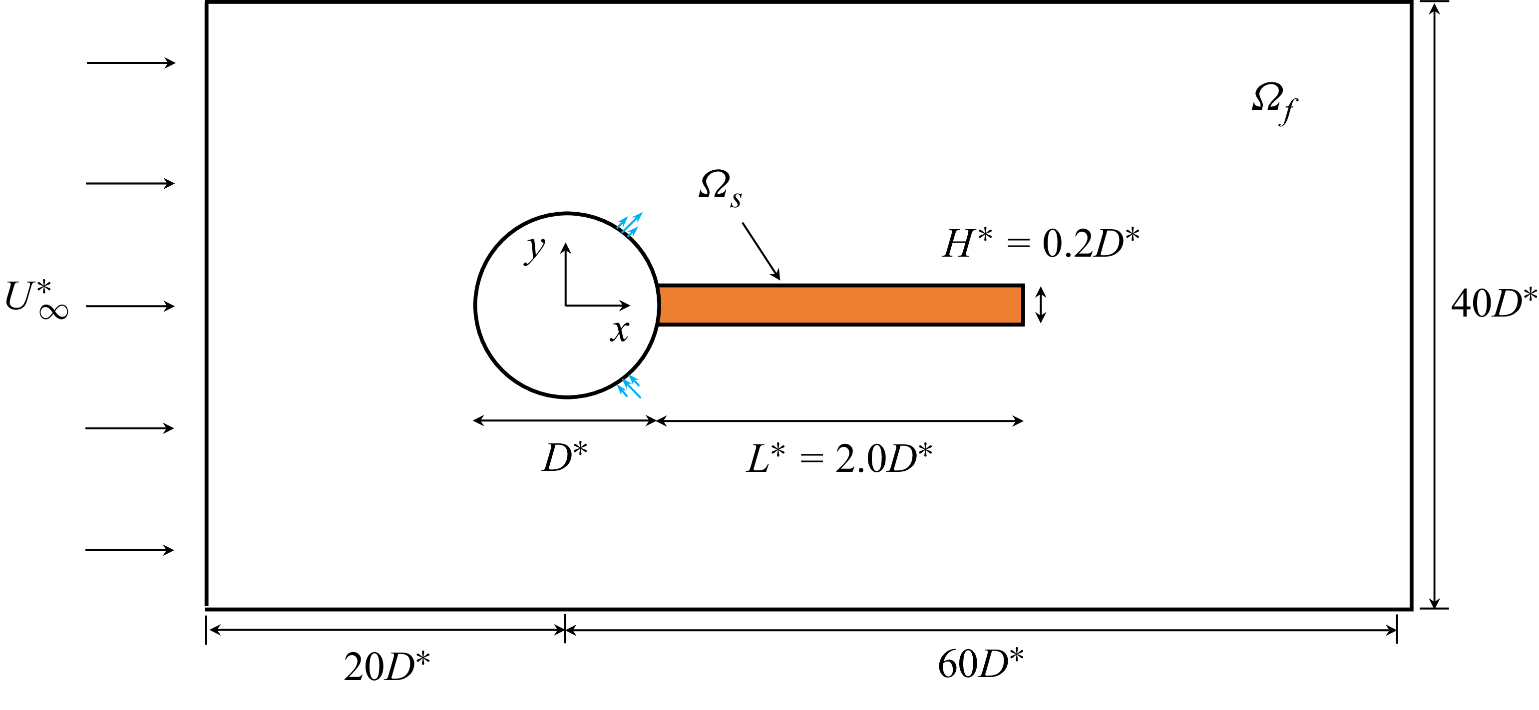
. Superscript (*) represents the dimensional variables. As shown in figure 1, the plate is clamped on the right-hand side of a rigid circular cylinder of diameter
 $D^*$
. A Cartesian coordinate system with its origin at the centre of the cylinder is used. The
 $x$
coordinate aligns with the streamwise direction, whereas the
 $y$
coordinate corresponds to the lateral direction.
Schematic of the elastic plate (orange shaded region) clamped to a rigid cylinder (white circle) and immersed in a uniform incoming flow. Blowing-suction actuators (blue arrows) are mounted on the cylinder.

The fluid is characterised by density
 $\rho _f^*$
and dynamic viscosity
 $\mu ^*$
. The structure is assumed homogeneous of density
 $\rho _s^*$
, and its elasticity is defined by Young’s modulus
 $E_s^*$
and Poisson coefficient
 $v_s$
under the assumption of isotropy. Young’s modulus characterises the stiffness while the Poisson coefficient evaluates the ratio between transverse and axial strains. Next, we calculate Lamé coefficients
 \begin{equation} \lambda _s^* = \frac {E_s^*v_s}{(1+v_s)(1-2v_s)}, \quad \mu _s^* = \frac {E_s^*}{2(1+v_s)}. \end{equation}
To obtain the non-dimensional variables and governing equations, we take
 $L^*$
and
 $U_{\infty }^*$
as the characteristic length and velocity. Then, we can define the non-dimensional Lamé coefficients as
 $\lambda _s = \lambda _s^*/(\rho _f^* U_{\infty }^{*2})$
and
 $\mu _s = \mu _s^*/(\rho _f^* U_{\infty }^{*2})$
. The flapping dynamics of the plate is strongly influenced by non-dimensional parameters, namely Reynolds number
 ${\textit{Re}}$
, and the density ratio
 $M$
, which are defined as
 \begin{equation} {\textit{Re}}=\frac {{{\rho }_{\!f}^*}{{U}_{\infty }^*}D^*}{\mu ^* },\qquad M=\frac {{{\rho }_{s}^*}}{{{\rho }_{\!f}^*}}, \end{equation}
where
 $M$
is the relative importance of solid-to-fluid inertia (Sader et al. Reference Sader, Cossé, Kim, Fan and Gharib2016). In this work, we fix
 $H^* = 0.2D^*$
.
The non-dimensional governing equation of this FSI problem includes the fluid sub-problem, solid sub-problem, extension sub-problem and boundary conditions in an arbitrary ALE reference frame. The extension sub-problem is introduced in the ALE method to propagate the structure displacement at the fluid–structure interface into the fluid domain. First, the Navier–Stokes equations governing an incompressible flow are
 \begin{align}&\qquad\qquad\qquad\qquad\qquad \boldsymbol{\nabla } \boldsymbol{\cdot }\left [ \boldsymbol{\varPhi }\! \left ( {{\eta }_{e}} \right )\boldsymbol{u} \right ]=0 \quad \textrm{in} \ {{\varOmega }_{\!f}}, \end{align}
 \begin{align}& J\!\left ( {{\eta }_{e}} \right )\frac {\partial \boldsymbol{u}}{\partial t}+\left [ \left ( \boldsymbol{\nabla }\boldsymbol{ u} \right )\boldsymbol{\varPhi } \!\left ( {{\eta }_{e}} \right ) \right ]\left ( \boldsymbol{u}-\frac {\partial {{\eta }_{e}}}{\partial t} \right )-\boldsymbol{\nabla } \boldsymbol{\cdot }\boldsymbol{\varSigma } \left ( \boldsymbol{u},p,{{\eta }_{e}} \right )=0 \quad \textrm{in} \ {{\varOmega }_{\!f}}, \end{align}
where
 ${\eta }_{e}$
is the extension displacement field used to describe the deformation of the fluid domain in a Lagrangian framework;
 $\boldsymbol{u} = (u_x, u_y)$
is the velocity of the fluid;
 $\boldsymbol{\varPhi } ( {{\eta }_{e}} )=J ( {{\eta }_{e}} ){{ ( \boldsymbol{I}+\boldsymbol{\nabla } {{\eta }_{e}} )}^{-1}}$
is the deformation operator, which expresses how an infinitesimal surface in the instantaneous configuration is transformed in the reference configuration (Aris Reference Aris2012);
 $\boldsymbol{I}$
is the unit matrix;
 $J ( {{\eta }_{e}} )$
is the transformation Jacobian. Here
 $\boldsymbol{\varSigma }$
is the first Piola-Kirchhoff stress tensor for the fluid, written as
 \begin{equation} \boldsymbol{\varSigma } \left ( \boldsymbol{u},p,{{\eta }_{e}} \right )=\left \{ -p\boldsymbol{I}+\frac {1}{{\textit{Re}}}\frac {1}{J\! \left ( {{\eta }_{e}} \right )}\left [ \left ( \boldsymbol{\nabla } \boldsymbol{ u} \right )\boldsymbol{\varPhi } \!\left ( {{\eta }_{e}} \right )+{{\left ( \boldsymbol{\nabla } \boldsymbol{u} \right )}^{T }}\boldsymbol{\varPhi } {{\!\left ( {{\eta }_{e}} \right )}^{T }} \right ] \right \}\boldsymbol{\varPhi } {{\left ( {{\eta }_{e}} \right )}^{T }}. \end{equation}
Then, the non-dimensional solid elasticity equation is defined as
 \begin{equation} {{M}}\frac {{{\partial }^{2}}{{\eta }_{s}}}{\partial {{t}^{2}}}-\boldsymbol{\nabla } \boldsymbol{\cdot }\left [ \boldsymbol{F} \!\left ( {{\eta }_{s}} \right )\boldsymbol{S} \!\left ( {{\eta }_{s}} \right ) \right ]=0 \quad \textrm{in} \ {{\varOmega }_{s}}, \end{equation}
where
 $\eta _s$
is the solid displacement field;
 $\boldsymbol{F} ( {{\eta }_{s}} )=\boldsymbol{I}+\boldsymbol{\nabla } {{\eta }_{s}}$
is the deformation gradient,
 $\boldsymbol{S} ( {{\eta }_{s}} )={{\lambda }_{s}}tr [ \boldsymbol{E} ( {{\eta }_{s}} ) ]\boldsymbol{I}+2{{\mu }_{s}}\boldsymbol{E} ( {{\eta }_{s}} )$
is the second Piola-Kirchhoff stress tensor written here for a compressible Saint-Venant–Kirchhoff material (Ogden Reference Ogden1997);
 $\boldsymbol{E} ( {{\eta }_{s}} )={1}/{2}\; [ \boldsymbol{F}{{ ( {{\eta }_{s}} )}^{T}}\boldsymbol{F} ( {{\eta }_{s}} )-\boldsymbol{I} ]$
is the Green–Lagrange strain tensor.
Next, the extension sub-problem is defined as
 \begin{align}& \boldsymbol{\nabla } \boldsymbol{\cdot }{{\boldsymbol{\varSigma } }_{e}}\!\left ( {{\eta }_{e}} \right )=0 \quad \textrm{in} \ {{\varOmega }_{\!f}}, \end{align}
 \begin{align}&\quad {{\eta }_{e}}-{{\eta }_{s}}=0 \quad \textrm{on} \ \varGamma , \end{align}
where
 $\varGamma$
is the interface of fluid and structure;
 ${\boldsymbol{\varSigma } }_{e}$
is the extension operator and the Laplace equation is used here (Helenbrook Reference Helenbrook2003) in order to ensure a smooth propagation of large deformation.
Finally, the velocity and stress continuity at the fluid–structure interface give
 \begin{align}&\qquad\qquad\quad \boldsymbol{u}-\frac {\partial {{\eta }_{e}}}{\partial t}=0 \quad \textrm{on}\ \varGamma , \end{align}
 \begin{align}& \boldsymbol{\varSigma } \left ( \boldsymbol{u},p,{{\eta }_{e}} \right )\boldsymbol{n}-\left [ \boldsymbol{F}\!\left ( {{\eta }_{s}} \right )\boldsymbol{S} \!\left ( {{\eta }_{s}} \right ) \right ]\boldsymbol{n}=0 \quad \textrm{on}\ \varGamma , \end{align}
where
 $\boldsymbol{n}$
represents the unit outward normal vector to the structural surface.
The flow control system employs a pair of symmetrically positioned blowing and suction jets along the
 $x$
axis (Rabault et al. Reference Rabault, Kuchta, Jensen, Réglade and Cerardi2019). The upper actuator is oriented at an angle of
 $\theta \in [\theta _1,\theta _2]$
with respect to the
 $x$
axis, while the lower actuator is positioned symmetrically. Each jet has a width of
 $\Delta w = \theta _2-\theta _1$
and discharges horizontally at its outlet. The velocity boundary conditions for both jets are prescribed as
 \begin{align} \boldsymbol{u}_{\textit{upper}} &= (u_x, u_y) = Q_{\textit{upper}}\left [\cos \left (\frac {\pi }{\Delta w}(\theta -{\theta _0})\right )\!, \cos \left (\frac {\pi }{\Delta w}(\theta -{\theta _0})\right )\right ]\!, \end{align}
 \begin{align} \boldsymbol{u}_{\textit{lower}} &= (u_x, u_y) = Q_{\textit{lower}}\left [\cos \left (\frac {\pi }{\Delta w}(\theta +\theta _0+\pi /2)\right )\!, {-}\cos \left (\frac {\pi }{\Delta w}(\theta +\theta _0+\pi /2)\right )\right ]\!, \end{align}
where the flow rate magnitude
 $Q_{\textit{upper}}$
and
 $Q_{\textit{lower}}$
are regulated by the MPC controller, the condition
 $Q_{\textit{upper}}+Q_{\textit{lower}}=0$
is enforced to ensure that there is no additional mass added to the flow. Here
 $\theta _0 = (\theta _1+\theta _2)/2$
is the radian of the upper jet centre and the values of
 $\theta _1$
and
 $\theta _2$
are defined according to the result of resolvent analysis in Appendix A.
2.2. Koopman reduced-order modelling for autonomous system
The control equations for the full-order FSI system presented above can be written in a more compact form, i.e.
 \begin{equation} \frac {\partial \boldsymbol{x}}{\partial t} = \boldsymbol{R}[\boldsymbol{x}( t),u(t)], \end{equation}
where the state variable
 $\boldsymbol{x}= (\boldsymbol{u},p,\eta _s, \eta _e) \in \mathcal{X}\subseteq \mathbb{R}^n$
represents the full state of the FSI system, encompassing the fluid, structure and extension variables. Here
 $\mathcal{X}$
is the corresponding state space and
 ${u}(t)\in \mathcal{U}$
is the control variable. The system dynamics is defined by
 $\boldsymbol{R}{:}\mathcal{X}\times \mathcal{U}\to \mathcal{X}$
, which acts on the full FSI state. After space and time discretisation, we obtain a discrete-time system of the form
 \begin{equation} {\boldsymbol{y}_{m}}=F \!\left ( {\boldsymbol{x}_{m}}, {u}_m \right )\!,\quad m\geqslant 0, \end{equation}
where
 $F:\varOmega \to \varOmega$
is the discrete form of the operator
 $\boldsymbol{R}$
and its application evolves the full-order FSI system by one time step. For the autonomous system,
 ${u}_m$
is a fixed value input, i.e. a constant jet boundary condition at the actuators. At the
 $m$
th time step the system is in state
 $\boldsymbol{x}_m$
, and we denote the initial state
 $\boldsymbol{x}_0$
. The Koopman operator
 $\mathcal{K}$
is defined by its action on functions
 $g \in \mathcal{H}$
:
 $\varOmega \to \mathbb{C}$
by the composition formula
 \begin{equation} \mathcal{K}g=g\circ F, \end{equation}
where
 $\mathcal{H} = L^2(\varOmega , \omega )$
is the Hilbert space and
 $\omega$
is a positive measure with
 $||\omega ||_{\varOmega } = \int _{\varOmega }\omega (\boldsymbol{x}) {\rm d}\boldsymbol{x}= 1$
(Williams et al. Reference Williams, Kevrekidis and Rowley2015). The Koopman operator defines a new dynamical system
 $(\mathcal{H},m,\mathcal{K})$
, compared with the original dynamical system
 $(\varOmega ,m,F)$
. When the Koopman operator is applied to a discrete state of the system, (2.15) reads
 \begin{equation} \left [ \mathcal{K}g \right ] \!\left ( {\boldsymbol{x}_{m}} \right )=g\! \left ( F \!\left ( {\boldsymbol{x}_{m}} \right ) \right )=g \!\left ( {\boldsymbol{y}_{m}} \right )\!, \end{equation}
i.e. the Koopman operator
 $\mathcal{K}$
transforms the nonlinear dynamics in the state variable
 $\boldsymbol{x}$
into an equivalent linear dynamics in the observable
 $g$
.
To determine
 $\mathcal{K}$
from measurement data, we use the KDMD algorithm (Williams, Rowley & Kevrekidis Reference Williams, Rowley and Kevrekidis2016), which constructs a matrix
 $\mathbb{K} \in \mathbb{C}^{N\times N}$
that approximates
 $\mathcal{K}$
on a finite-dimensional subspace
 ${{V}_{N}}=\textrm{span}\left \{ {{\psi }_{1}},\cdots ,{{\psi }_{N}} \right \}$
generated by a set of basis observable functions
 $\psi _{\!j}:\varOmega \to \mathbb{C}$
, whose specific form will be specified later. Let us define the vector-valued observable
 $\varPsi (\boldsymbol{x} )= [ {{\psi }_{1}} ( \boldsymbol{x} )\textrm{ }\cdots \textrm{ }{{\psi }_{N}} ( \boldsymbol{x} ) ]\in {{\mathbb{C}}^{1\times N}}$
, any observable
 $g \in V_N$
can be written as
 \begin{equation} g ( \boldsymbol{x})=\sum \limits _{j=1}^{N}{{{\psi }_{j}} ( \boldsymbol{x} ){{a}_{j}}=\varPsi } ( \boldsymbol{x} )\boldsymbol{a}, \end{equation}
where the
 $a_{\!j}$
are projection coefficients. In general,
 $\mathcal{K}g \notin V_N$
. So, inserting (2.17) in (2.16) gives
 \begin{equation} \left [ \mathcal{K}g \right ]( \boldsymbol{x})=\varPsi \left [ F(\boldsymbol{x}) \right ]\boldsymbol{a}=\varPsi (\boldsymbol{x})\left ( \mathbb{K}\boldsymbol{a} \right )+R\left ( \boldsymbol{a},\boldsymbol{x} \right )\!, \end{equation}
where
 $R$
is a residual quantity that reads
 \begin{equation} R( \boldsymbol{a},\boldsymbol{x}) = \sum \limits _{j=1}^{N}{{{\psi }_{j}} \!\left [ F(\boldsymbol{x}) \right ]{{a}_{j}}-\varPsi }(\boldsymbol{x}) ( \mathbb{K}\boldsymbol{a}). \end{equation}
The subspace
 $V_N$
generated by the dictionary is not an invariant subspace of
 $\mathcal{K}$
, and hence, there is no choice of
 $\mathbb{K}$
that makes the error
 $R(\boldsymbol{a},\boldsymbol{x})$
zero. Instead, it is natural to select
 $\mathbb{K}$
as to minimise
 \begin{equation} \int _\varOmega \max _{\|\boldsymbol{a}\|=1} |R(\boldsymbol{a},\boldsymbol{x})|^2 {\textrm d}\omega (\boldsymbol{x}) = \int _\varOmega \|\varPsi (F(\boldsymbol{x})) - \varPsi (\boldsymbol{x})\mathbb{K}\|^2 {\textrm d}\omega (\boldsymbol{x}), \end{equation}
where
 $\|\boldsymbol{\cdot }\|$
denotes the standard Euclidean norm. Given a finite amount of snapshot data, we cannot directly evaluate the integral in (2.20). Instead, the matrix
 $\mathbb{K}$
is then defined as the one that minimises (in a least-squares sense) the residual evaluated over the data samples. The minimisation problem reads
 \begin{equation} \mathbb{K} = \underset {B\in {{\mathbb{C}}^{N\times N}}}{\mathop {\arg \min }}\,\sum \limits _{m=1}^{M}{{{w}_{m}} {{\left \| \varPsi \! \left ( {\boldsymbol{y}_{ m}} \right )-\varPsi \! \left ( {\boldsymbol{x}_{ m }} \right ) \! B \right \|}^{2}}}, \end{equation}
where
 $w_m$
is the weighting factors and we take it equal to
 $1/M$
for the present ergodic sampling method according to the suggestion of Colbrook et al. (Reference Colbrook, Ayton and Szőke2023). Then, defining the following two data matrices containing the measurement data ‘processed’ by the basic functions
 $\psi$
,
 \begin{equation} {{\varPsi }_{X}}=\left [ \begin{matrix} \varPsi \!\left ( {\boldsymbol{x}_{1}} \right ) \\ \vdots \\ \varPsi \! \left ( {\boldsymbol{x}_{M}} \right ) \\ \end{matrix} \right ]_{M \times N}, \qquad {{\varPsi }_{Y}}=\left [ \begin{matrix} \varPsi \! \left ( {\boldsymbol{y}_{1}} \right ) \\ \vdots \\ \varPsi \! \left ( {\boldsymbol{y}_{M}} \right ) \\ \end{matrix} \right ]_{M \times N}, \end{equation}
where
 $\varPsi _X \in {{\mathbb{C}}^{M\times N}}$
and
 $\varPsi _Y \in {{\mathbb{C}}^{M\times N}}$
, it can be shown that the solution of (2.21) is (Williams et al. Reference Williams, Rowley and Kevrekidis2016)
 \begin{equation} \mathbb{K} ={{\big ( \varPsi _{X}^{T}W{{\varPsi }_{X}} \big )}^{+ }}\big ( \varPsi _{X}^{T}W{{\varPsi }_{Y}} \big )={{\big ( \sqrt {W}{{\varPsi }_{X}} \big )}^{+ }}\big ( \sqrt {W}{{\varPsi }_{Y}} \big ), \end{equation}
where
 $W={\textit{diag}} ( {{w}_{1}},\textrm{ }\cdots \textrm{ },{{w}_{M}} )$
is the diagonal weight matrix and ‘
 $+$
’ denotes the pseudoinverse. To reduce the computational burden of (2.23), we define
 $\psi$
implicitly and apply the kernel trick by defining a kernel function
 $\boldsymbol{f}$
that computes inner products in feature space given pairs of data points, i.e.
 \begin{equation} \boldsymbol{f}(\boldsymbol{x}_i, \boldsymbol{x}_{\!j}) = {\psi }(\boldsymbol{x}_{\!j})^T{\psi }(\boldsymbol{x}_i), \end{equation}
where
 $\boldsymbol{f}$
does not compute these inner products directly. Furthermore, we induce the Gaussian kernels as
 \begin{equation} \boldsymbol{f}(\boldsymbol{x}_i,\boldsymbol{y}_{\!j}) = \textrm{e}^{-||\boldsymbol{x}_i - \boldsymbol{y}_{\!j}||^2 / \sigma ^2}, \end{equation}
which has a good performance both in terms of numerical conditioning and in approximating the Koopman operator in fluid mechanics (Ham et al. Reference Ham, Lee, Mika and Schölkopf2004). Gaussian kernels also show effectiveness for the present FSI reduced-order modelling. Here
 $\sigma$
is the hyperparameter. After taking expression (2.24) into (2.23), we can calculate the Koopman matrix
 $\mathbb{K}$
with lower memory consumption. Moreover,
 $\psi (\boldsymbol{x})$
can be written as (Williams et al. Reference Williams, Rowley and Kevrekidis2016)
 \begin{equation} \psi _{k}(\boldsymbol{x}) = [\boldsymbol{f}(\boldsymbol{x},\boldsymbol{x}_1), \boldsymbol{f}(\boldsymbol{x},\boldsymbol{x}_2), \cdots , \boldsymbol{f}(\boldsymbol{x},\boldsymbol{x}_M)](U\varSigma ^{+})q_k,\quad k = 1,\ldots ,N, \end{equation}
where
 $U_{M\times M}$
is a unitary matrix and
 $\varSigma _{M \times M}$
is a diagonal matrix obtained by SVD:
 $\sqrt {W}\varPsi _X = U \!\varSigma\! Q^T$
. Next, we can compute the Koopman eigenfunctions and modes as (Colbrook et al. Reference Colbrook, Ayton and Szőke2023)
 \begin{equation} \boldsymbol{x}\approx \underbrace {\varPsi (\boldsymbol{x})V}_{\textrm{Koopman}\textrm{ eigenfunctions}}\underbrace {\left [ {{V}^{-1}}{{\big ( \sqrt {W}{{\varPsi }_{X}} \big )}^{\dagger }}\sqrt {W}{{\left [ {\boldsymbol{x}_{1}}\textrm{ }\cdots \textrm{ }{\boldsymbol{x}_{M}} \right ]}^{T}} \right ]}_{N\times d\textrm{ matrix of Koopman modes}}, \end{equation}
where the matrix
 $V = [v_1, v_2, \ldots ,v_N]$
represents eigenvectors and
 $\varLambda = \textit{diag}(\lambda _1, \lambda _2,\ldots ,\lambda _N)$
is a diagonal matrix of eigenvalues from the eigen-decomposition of the Koopman matrix
 $\mathbb{K}$
as
 $\mathbb{K}V=\varLambda V$
. The
 $j$
th Koopman mode corresponds to the
 $j$
th row of the matrix in square brackets, and
 $\varPsi V$
is a quasimatrix of an approximate Koopman eigenfunction.
Although we obtain eigenvalue-eigenvector pairs
 $(\lambda _i,v_i)$
that form the Koopman matrix
 $\mathbb{K}$
from the KDMD method detailed above, it cannot be used to verify the accuracy of these pairs. For this, Colbrook et al. (Reference Colbrook, Ayton and Szőke2023) proposed the ResDMD algorithm, which uses an additional matrix constructed from the measured data,
 $ \{ {\boldsymbol{x}_{m}},{\boldsymbol{y}_{m}} \}_{m=1}^{M}$
. ResDMD constructs Galerkin approximations for both
 $\mathcal{K}$
and
 $\mathcal{K}*\mathcal{K}$
, which gives rigorous convergence guarantees for ResDMD and determines which part of the computed spectra and Koopman modes are reliable. By defining the squared relative residual as
 \begin{equation} \mathop {\textrm{lim}}\limits _{M \rightarrow \infty } \textit{res}(\lambda ,v)^2=\frac {\int _{\varOmega }|[\mathbb{K}v(\boldsymbol{x}) - \lambda v(\boldsymbol{x})]|^2 \textrm{d}\omega (\boldsymbol{x})}{\int _{\varOmega }|v(\boldsymbol{x})|^2 \textrm{d}\omega (\boldsymbol{x})}, \end{equation}
where
 $v = \varPsi \boldsymbol{v}$
. This residual can be approximate by using the quadrature rule as
 \begin{equation} \textit{res}{{\left ( \lambda ,\boldsymbol{v} \right )}^{2}}=\frac {{\boldsymbol{v}^{T}} \!\left [ \varPsi _{Y}^{T}W{{\varPsi }_{Y}}-\lambda {{\left [ \varPsi _{X}^{T}W{{\varPsi }_{Y}} \right ]}^{T}}-\overline {\lambda } \varPsi _{X}^{T}W{{\varPsi }_{Y}}+{{\left | \lambda \right |}^{2}}\varPsi _{X}^{T}W{{\varPsi }_{X}} \right ]\boldsymbol{v}}{{\boldsymbol{v}^{T}} \!\left [ \varPsi _{X}^{T}W{{\varPsi }_{X}} \right ] \!\boldsymbol{v}}. \end{equation}
The matrices
 $\varPsi _{X}^{T}W{{\varPsi }_{X}}$
and
 $\varPsi _{X}^{T}W{{\varPsi }_{Y}}$
are the same with the KDMD, and we only need to calculate the additional matrix
 $\varPsi _{Y}^{T}W{{\varPsi }_{Y}}$
. In this work, we employ the ResDMD algorithm to eliminate pseudo-modes and enhance the accuracy of Koopman reduced-order modelling.
2.3. Koopman ROM-based MPC
Next, we implement control through switched systems techniques, which couple a finite set of autonomous Koopman ROMs (§ 2.2) with the MPC algorithm. Our overall objective is to effectively suppress the instability of a flexible plate, and the objective function can be formulated as follows:
 \begin{equation} \mathcal{J} = \min _{{u} \in L^2([t_0,t_e],\mathbb{R}^r)} \int _{t_0}^{t_e} \mathcal{F}[\boldsymbol{\delta }(t), {u}(t)] {\textrm d}t \quad \textrm{with} \quad \begin{cases} \dfrac {\partial \boldsymbol{x}}{\partial t} = \boldsymbol{R}[\boldsymbol{x}( t),u(t)], \\ \boldsymbol{x}(t_0) = \boldsymbol{x}_0. \end{cases} \end{equation}
Here
 $\mathcal{J}$
is the objective function and
 $r$
is the number of control degrees of freedom. The objective of the control is to suppress the flapping of the plate. Therefore, the target variable
 $\boldsymbol{\delta }(t)$
, which represents the displacement of the plate captured by strategically positioned probes, is a structural sub-portion of the full-state vector
 $\boldsymbol{x}(t)$
. The objective adopts a standard regulation form
 $\mathcal{F}[\boldsymbol{\delta }(t),{u}(t)]=\|\boldsymbol{\delta }(t) - \boldsymbol{\delta }^{\textit{ref}}(t)\|^2$
. This formulation aims to regulate the plate’s displacement to a reference value
 $\boldsymbol{\delta }^{\textit{ref}}(t)$
.
We use the MPC algorithm (Grüne et al. Reference Grüne, Pannek, Grüne and Pannek2017) to solve the above optimisation problems over finite prediction horizons, enabling continuous adaptation to changing system states and environmental conditions. Specifically, this approach utilises a finite prediction horizon spanning from
 $t_0$
to
 $t_e$
(with length
 $t_p=t_e-t_0$
) to forecast system behaviour. Furthermore, only an initial segment of duration
 $ t_c$
(where
 $t_c \leqslant t_{p}$
) from the solution of (2.30) is actually applied to the system. Simultaneously, the optimisation process is continuously repeated, with each iteration shifting the prediction window forward by
 $ t_c$
, creating a receding-horizon implementation. Based on the approach in Peitz, Otto & Rowley (Reference Peitz, Otto and Rowley2020), we first replace the dynamical control system in (2.30) by a finite number of
 $n_c$
autonomous systems,
 \begin{equation} \boldsymbol{R}_{\bar {u}}(\boldsymbol{x})=\boldsymbol{R}(\boldsymbol{x},\bar {u}), \end{equation}
with constant input
 $\bar {{u}}\in \tilde {\mathcal{U}}=\{\bar {{u}}_1,\ldots ,\bar {{u}}_{n_c}\}$
; and problem (2.30) is transformed into a switching problem, where the objective is to select the optimal right-hand side in each time step:
 \begin{equation} \mathcal{J} = \min _{ {u}(t)\in \tilde {\mathcal{U}}} \int _{t_0}^{t_e} \mathcal{F}[\boldsymbol{\delta }(t), {u}(t)] {\textrm d}t \\ \quad \textrm{with} \quad \begin{cases} \dfrac {\partial \boldsymbol{x}}{\partial t} = \boldsymbol{R}_{{u}(t)}(\boldsymbol{x}(t)), \\ \boldsymbol{x}(t_0) = \boldsymbol{x}_0. \end{cases} \end{equation}
This problem differs from (2.30) in that
 $\mathcal{U}$
is replaced by
 $\tilde {\mathcal{U}}$
, and the dynamics is now governed by
 $\boldsymbol{R}_{{u}(t)}$
. In other words,
 ${u}(t)$
describes which system
 $\boldsymbol{R}_{\bar {{u}}_{\!j}}$
,
 $j \in \{1,\ldots ,n_c\}$
, to apply at time
 $t$
.
To facilitate numerical implementation, we transform the continuous-time optimal control problem into a discrete-time formulation. We partition the time interval
 $[t_0, t_e]$
into
 $p$
equidistant subintervals with constant time step
 $t_c = t_{i+1} - t_i$
,
 $i = 0, 1, \ldots , p-1$
. Specifically, we assume the control input
 ${u}(t) = {u}_i \in \tilde {\mathcal{U}}$
remains constant over each interval
 $[t_i, t_{i+1}]$
, which leads to
 \begin{equation} \boldsymbol{x}_{i+1} = F(\boldsymbol{x}_i,{u}_i)=\boldsymbol{x}_i+\int _{t_i}^{t_{i+1}}\boldsymbol{R}[\boldsymbol{x}(t),{u}_i]{\textrm d}t, \end{equation}
where
 $\boldsymbol{x}_i$
represents the system state at time
 $t_i$
. Using the above considerations, we compute
 $n_c$
distinct Koopman operators corresponding to
 $n_c$
different autonomous systems, enabling efficient characterisation and prediction of system dynamics (2.33), as
 \begin{equation} \left [ \mathcal{K}_{{\bar {u}}_{\!j}}g \right ](\boldsymbol{x})=\varPsi (F_{{\bar {u}}_{\!j}}(\boldsymbol{x}))\boldsymbol{a},\quad j=1,\ldots ,n_c, \end{equation}
where
 $F_{{\bar {u}}_{\!j}}$
is now the family of flow maps corresponding to the fixed control inputs
 ${\bar {u}}_{\kern-1pt j}$
. Using Koopman reduced-order modelling in § 2.2, we can compute the approximations of the individual Koopman operators from the observations of each system. The continuous control inputs are approximated using a zero-order hold with a constant input over each interval of length
 $t_c$
. This discretisation replaces the original dynamics in (2.32), resulting in the following problem over a prediction range of length
 $pt_c$
(i.e.
 $p$
steps of size
 $t_c$
):
 \begin{equation} \hat {\mathcal{J}} = \min _{{u}_{0}, \ldots , {u}_{p-1}\in \tilde {\mathcal{U}}} \sum _{i=0}^{p-1}\hat {\mathcal{F}}_{i+1}(\tilde {\boldsymbol{\delta }}_{i+1}, u_{i+1}), \quad \textrm{with} \quad \begin{cases} g(\tilde {\boldsymbol{\delta }}_{i+1}) = \mathcal{K}_{\bar {{u}}_{\!j}}g(\tilde {\boldsymbol{\delta }}_i), \\[6pt] i = 0, 1, 2, \ldots , p-1. \end{cases} \end{equation}
Here
 $\hat {\mathcal{J}}$
is the overall objective function over the time horizon
 $T = p\Delta t$
and
 $\hat {\mathcal{F}}$
is the objective function at a particular time instant, i.e. a tracking term
 $\hat {\mathcal{F}}_{i+1}(\tilde {\boldsymbol{\delta }}_{i+1}, u_{i+1})=\|\tilde {\boldsymbol{\delta }}_{i+1} - \boldsymbol{\delta }_{i+1}^{\textit{ref}}\|^2$
;
 $\tilde {\boldsymbol{\delta }}$
is the reconstructed displacement obtained by (2.27). Finally, we optimisation using relaxation techniques (Nocedal & Wright Reference Nocedal and Wright1999), which yield a continuous approximation of the original problem that can be efficiently solved using nonlinear constrained optimisation methods.
As a first step towards the relaxation of (2.35), we introduce a control variable
 $\omega \in (\{0,1\}^{n_c})^{p}$
that yields a formulation equivalent to (2.35), i.e.
 \begin{equation} \begin{aligned} & \hat {\mathcal{J}} = \min _{\boldsymbol{\omega }\in (\{0,1\}^{n_c})^{p}} \sum _{i=0}^{p-1} \hat {\mathcal{F}}_{i+1}(\tilde {\boldsymbol{\delta }}_{i+1},u_{i+1}), \\ \textrm{with} & \quad \begin{cases} g(\tilde {\boldsymbol{\delta }}_{i+1}) = \sum _{j=1}^{n_c} \omega _{i,j}\mathcal{K}_{\bar {{u}}_{\!j}}g(\tilde {\boldsymbol{\delta }}_i), \\[6pt] \sum _{j=1}^{n_c} \omega _{i,j} = 1, \quad i = 0, 1, 2, \ldots , p-1, \end{cases} \end{aligned} \end{equation}
where
 $i = 0, 1, 2, \ldots , p-1$
. The optimisation problem in (2.36) involves discrete binary control inputs (
 $\omega _{i,j}\in \{0,1\}$
), which can be computationally expensive to solve. To enable a more efficient solution, we relax this discrete problem into a continuous optimisation problem. This relaxation is achieved by replacing the binary variables
 $\omega _{i,j}$
with continuous variables
 $\alpha _{i,j}$
that are constrained to the interval [0, 1]. The resulting relaxed problem is formulated as
 \begin{equation} \begin{aligned} &\hat {\mathcal{J}} = \min _{\boldsymbol{\alpha }\in ([0,1]^{n_c})^{p}} \sum _{i=1}^{p} \hat {\mathcal{F}}_{i+1}(\tilde {\boldsymbol{\delta }}_{i+1},u_{i+1}), \\ \textrm{with} &\quad \begin{cases} g(\tilde {\boldsymbol{\delta }}_{i+1}) = \sum _{j=1}^{n_c} \alpha _{i,j}\mathcal{K}_{\bar {{u}}_{\!j}}g(\tilde {\boldsymbol{\delta }}_i), \\[7pt] \sum _{j=1}^{n_c} \alpha _{i,j} = 1, \quad i = 0, 1, 2, \ldots , p-1. \end{cases} \end{aligned} \end{equation}
To solve (2.37), we use BFGS methods for nonlinear optimisation (Nocedal & Wright Reference Nocedal and Wright1999). We can then apply input
 $u_i = \sum _{j=1}^{n_c}\alpha _{i,j}\bar {u}_{\!j}, i = 0,1,2,\ldots$
to the full-order system.
Schematic of the Koopman-based MPC control framework. The process involves three main steps: (a) collecting data from the FOM; (b) constructing ROMs using KDMD and ResDMD; and (c) implementing switched-system Koopman-MPC control. Flow field snapshots from
 $T_1$
to
 $T_n$
illustrate the evolution of the controlled FSI system.

The real-time control process is shown in figure 2, consisting of three steps. First, the complete training sequence
 $U_{{Input}}$
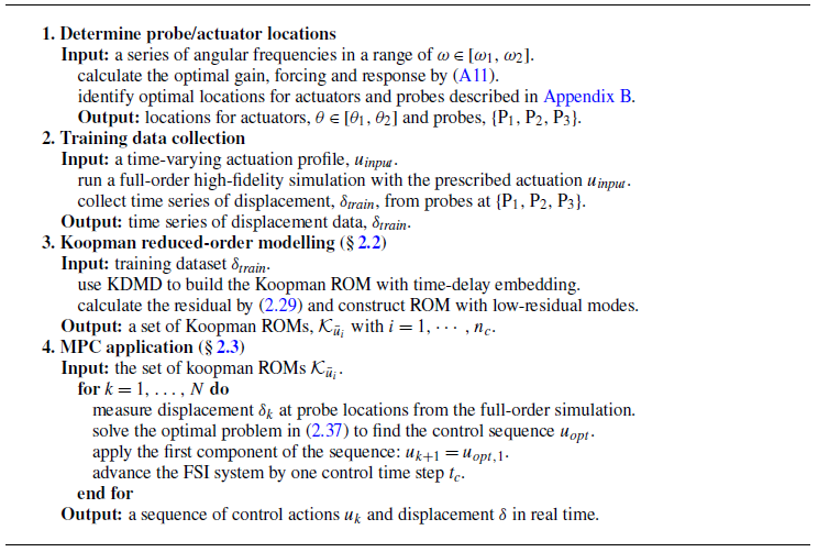
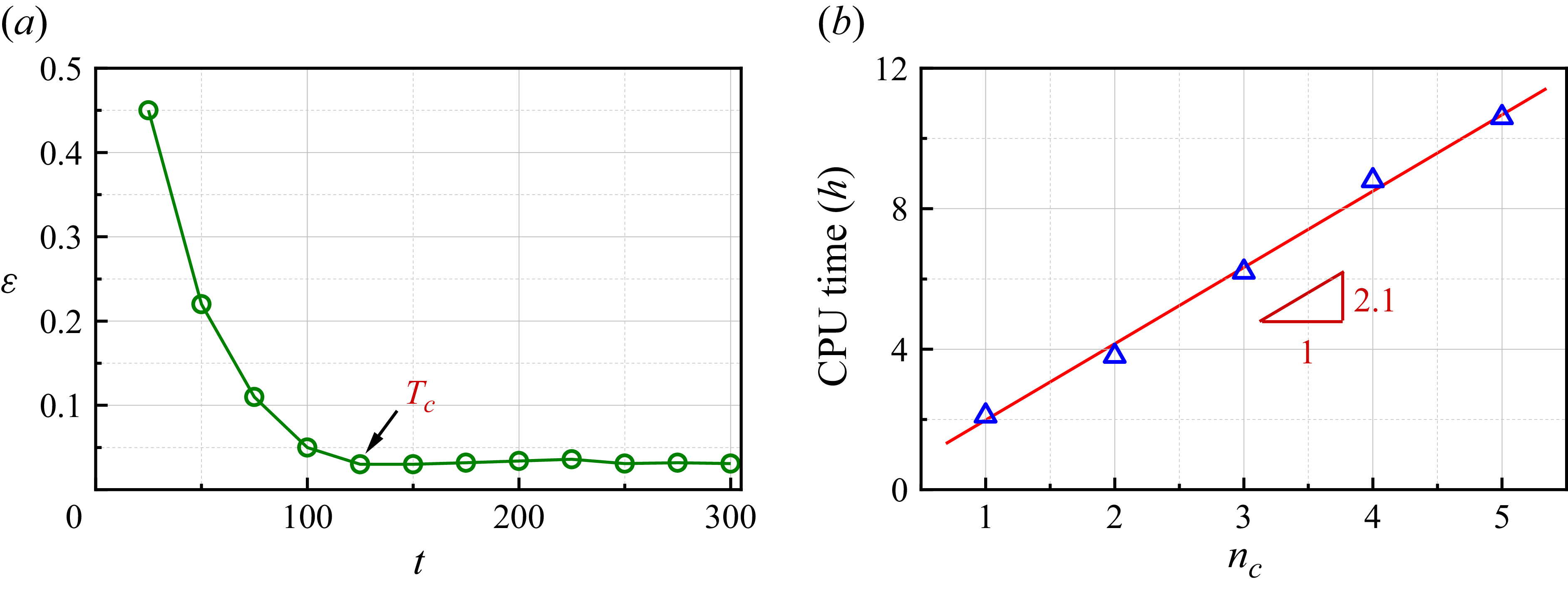
is applied to the FOM through actuators, and displacement data are collected at measurement points using probes. Next, we perform high-precision reduced-order modelling for each autonomous system using KDMD and ResDMD methods, and validate the results against real data. Finally, we implement active control of the FOM based on a switched system with relaxation control algorithms under the MPC framework. The detailed procedure is shown in Algorithm 1.
Control algorithm

3. Results and discussions
In this section we first examine the hydrodynamic response of the uncontrolled FSI system and characterise its behaviour across varying Young’s moduli
 $E_s$
. Then, a Koopman-based ROM is constructed and assessed in terms of accuracy and computational efficiency. The model is integrated with a MPC framework and applied to the full-order FSI system to suppress plate instability. Finally, we evaluate the control performance and elucidate the underlying mechanisms through Koopman mode decomposition and energy transfer analysis.
3.1. Vibration modes in uncontrolled FSI system under varying stiffness
Numerical simulations of (2.3)–(2.8) are performed with a fixed Reynolds number, solid-to-fluid density ratio and Poisson’s ratio, while varying the non-dimensional Young’s modulus, such that
 \begin{equation} \textit{Re} = 150, \quad M = 1, \quad v_s = 0.35, \quad 2\times 10^4 \leqslant E_s \leqslant 6\times 10^6. \end{equation}
The selected parameter regime is chosen to explore a novel flapping regime, distinct from yet comparable to those in previous studies. Although we adopt the same Reynolds numbers as in Wu et al. (Reference Wu, Qiu, Shu and Zhao2014), our study employs a flexible splitter plate set-up instead of a filament. Furthermore, the range of Young’s modulus investigated is also novel, differing from that studied by Lee & You (Reference Lee and You2013) (
 $1.61\times 10^4 \leqslant E_s\leqslant 9.66 \times 10^4$
). The choice of
 $M = 1$
allows us to investigate instability mechanisms driven by FSI rather than by wake instabilities alone. Moreover, the regime investigated in this study corresponds to biological conditions observed in small aquatic organisms, such as ascidian and fish larvae (McHenry, Azizi & Strother Reference McHenry, Azizi and Strother2003; China et al. Reference China, Levy, Liberzon, Elmaliach and Holzman2017), which typically operate at low Reynolds numbers and density ratios near unity.
Three types of plate responses under different Young’s moduli: (a) large-amplitude flapping (LAF) at
 $E_s = 4\times 10^4$
, (b) small-deflected flapping (SDF) at
 $E_s = 4\times 10^5$
, and (c) small-amplitude flapping (SAF)
 $E_s = 4\times 10^6$
. The top row (ai–ci) shows snapshot of the plate in saturated oscillation phases. The bottom row (aii–cii) presents the corresponding phase-space trajectories over time from
 $t = 0$
to 300.

Snapshots of the vorticity field. Panel (a) is the solution before the onset of instability. Panels (b)–(d) correspond to the three representative flapping regimes in figure 3, i.e. LAF, SDF and SAF, respectively. The black lines with arrows represent the streamlines. Black lines with arrows indicate streamlines and blue arrows denote the flapping direction.

The simulations are initialised with a uniform zero flow field, and the inlet velocity is smoothly increased from zero to
 $U_{\infty }^*$
. As the flow develops, two symmetric (with respect to the
 $x$
axis) recirculating vortices form behind the cylinder, located above and below the elastic plate. These recirculating regions tend to slightly compress the elastic plate in the direction of
 $x \lt 0$
, leading the system to an undeflected equilibrium (UE) phase. Subsequently, self-excited instabilities emerge, giving rise to three different types of limit cycles, each corresponding to the selected
 $E_s$
:
 $4\times 10^4$
,
 $4\times 10^5$
and
 $4\times 10^6$
. To illustrate the characteristics of these three cases, figure 3 presents flow snapshots over one oscillation cycle in the saturated flapping phase (first row) along with phase portraits (second row) constructed from the plate tip displacement
 $\delta$
and the velocity
 ${\textrm d}\delta /{\textrm d}t$
over the time interval
 $0 \lt t \lt 300$
. For
 $E_s = 4 \times 10^4$
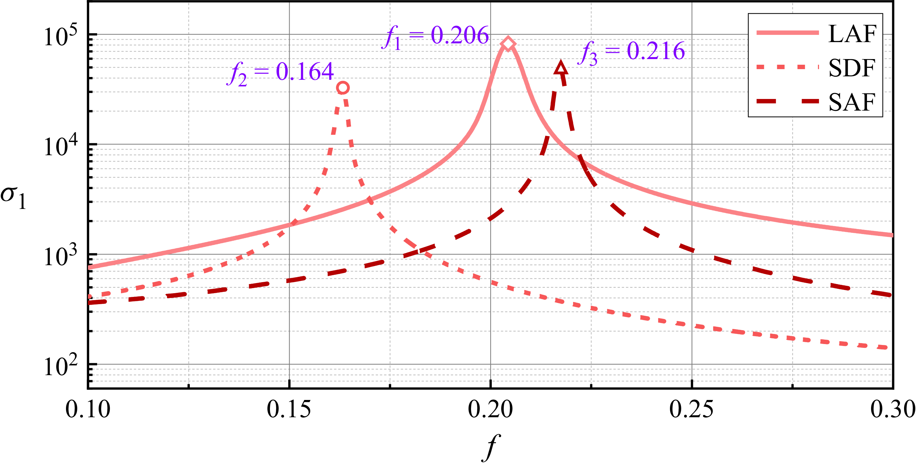
, an inflection point appears in the centreline deformation of the plate, and the maximum transverse deviation increases, causing the plate’s end to trace a characteristic figure-eight pattern as shown in figure 3(ai). This regime is referred to as large-amplitude flapping (LAF), characterised by displacement exceeding half the cylinder diameter. Moreover, the onset of instability exhibits characteristics of a Hopf bifurcation, with oscillatory behaviour emerging as the system becomes unstable, as shown in the phase trajectory in figure 3(aii). The system transitions to a limit-cycle state after
 $t \gt 160$
. Representative snapshots of the vorticity field during this regime are presented in figure 4(b). Two shear layers with opposite signs form on the upper and lower surfaces of the rigid cylinder, further shedding vortices in the downstream wake. The elastic plate interacts strongly with the larger vortex shedding, particularly near its trailing edge, where it appears to act as a ‘vortex cutter’, enhancing vortex detachment. This results in a ‘2S’ vortex shedding pattern that consists of two single vortices per cycle. The dominant flapping frequency in this regime is measured to be
 $f = 0.212$
. When the Young’s modulus increases to
 $E_s = 4 \times 10^5$
, small-deflected flapping (SDF) emerges, characterised by oscillations around an off-centre position deflected from the symmetry axis
 $y = 0$
. As illustrated in figure 3(bi), the plate deflects downward; however, a solution with upward deflection of the same magnitude can also be obtained. The selection between these two symmetric states is determined by the direction of the initial perturbation, which in a numerical simulation is implicitly introduced by factors such as the inherent micro-asymmetries of the computational mesh. The time evolution of
 $\delta$
shown in figure 3(bii) clearly displays the mean deflection. Between
 $t = 0$
and
 $t = 125$
, the plate tip gradually shifts downward without oscillation, a behaviour previously reported in numerical studies (Bagheri, Mazzino & Bottaro Reference Bagheri, Mazzino and Bottaro2012; Lācis et al. Reference Lācis, Brosse, Ingremeau, Mazzino, Lundell, Kellay and Bagheri2014). For
 $t \gt 125$
, oscillations emerge and grow exponentially, eventually saturating into a periodic limit cycle beyond
 $t \gt 220$
. The fundamental frequency is
 $f = 0.168$
and the oscillation amplitude is substantially smaller than that of the LAF mode. Consequently, the mean deflection exerts a significant stabilising effect on wake oscillations. Figure 4(c) presents snapshots of vorticity in the deflected limit cycle. The plate’s mean position consistently remains in the
 $y \lt 0$
region, with small oscillations superimposed. Vortices are released but with diminished intensity compared with LAF and at locations further from the plate surface. The ‘2S’ mode is absent, which suggests the overall more streamlined shape impedes vortex release in the wake. Moreover, a triangular lid-driven recirculation zone is formed between the rear of the cylinder and the plate, trapping a vortex
 $V^*$
that remains confined throughout the flapping cycle without escaping into the wake.
Figure 3(c) presents the small-amplitude flapping (SAF) regime at
 $E_s = 4\times 10^6$
. The oscillation initially grows exponentially, subsequently saturating into a periodic limit cycle after
 $t \gt 265$
. Unlike the SDF state, the plate returns to a symmetric flapping pattern, though with reduced amplitude and without centreline inflection, different from that observed under LAF conditions. The dominant flapping frequency is
 $f = 0.203$
. As illustrated in figure 4(d), the flow field also exhibits the ‘2S’ vortex shedding pattern, as
 $V^*$
is released and can enter the wake. A closer examination of the flow around the plate reveals that small secondary vortices emerge around the plate tip during motion: negative vorticity when the plate moves downward and positive vorticity when the plate moves upward. These vortices lack sufficient strength to separate and persist in the wake, but they generate enough downwash (or upwash) effects to influence the surrounding larger vortices.
Characteristics of the three flapping regimes obtained from direct numerical simulation. For different values of
 $E_s$
, panel (a) shows the transverse tip displacement
 $\delta$
of the plate in the limit-cycle regime. The mean displacement is computed as
 $\delta _{\textit{mean}} = 1/2(\delta _{\textit{max}}+\delta _{\textit{min}})$
, while the amplitude
 $\delta _{\textit{amp}} = 1/2(\delta _{\textit{max}}-\delta _{\textit{min}})$
is indicated by error bars centred at the mean. Panel (b) presents the first two main flapping frequencies
 $f_0$
and
 $f_1$
. The LAF, SDF and SAF regimes are highlighted with light yellow and purple and blue. The critical transition Young’s moduli between the three regimes are
 $E_{s1} = 1.26 \times 10^5$
and
 $E_{s2} = 7.78 \times 10^5$
.

To further explore the system behaviour over a broad range of Young’s modulus values, figure 5 summarises the flapping characteristics of the elastic plate in the saturated limit-cycle regime. Figure 5(a) shows the transverse tip displacement
 $\delta$
and figure 5(b) presents the first two dominant flapping frequencies
 $f_0$
and
 $f_1$
obtained via a fast Fourier transform. Moreover,
 $f_1$
is the second harmonic of
 $f_0$
(
 $f_1 = 2f_0$
). As
 $E_s$
increases, the system transitions through three distinct dynamical regimes. For low stiffness (
 $E_s \lesssim 1.26 \times 10^5$
), the system remains symmetric about the midline, with large flapping amplitudes (
 $\delta _{\textit{amp}} \gt 0.25$
) and zero-mean displacement, corresponding to the LAF regime. Beyond this critical value is the SDF regime, where the plate oscillates around an off-centred mean position (
 $\delta _{\textit{mean}} \lt 0$
) with lower frequencies (
 $f \lt 0.2$
) and reduced amplitudes. As the stiffness further increases beyond
 $E_s = 7.78 \times 10^5$
, the system regains symmetry, entering the SAF regime, characterised by weaker oscillations and the absence of large-scale wake interactions. For clarity in the subsequent analysis, we select
 $E_s = 4 \times 10^4$
,
 $4 \times 10^5$
and
 $4 \times 10^6$
as representative parameters of the LAF, SDF and SAF regimes, respectively.
3.2. Koopman reduced-order modelling
(a) Full input sequence
 $u_{{\textit{train}}}$
, where
 $D_1$
is used to construct the Koopman ROM and
 $D_2$
is used for validation. (b) A portion of
 $u_{{\textit{train}}}$
from
 $t= 200$
to
 $220$
; the blue shaded region represents an input corresponding to
 $\mathcal{K}_{\bar {u}_2}$
. (c) Displacement response at probe P
 $_3$
under the full input shown in (a). (d) A portion of displacement response under the input
 $\bar {u}_2 = 0.15$
only. The abscissa
 $t^*$
is a redefined continuous-time coordinate.

To construct the Koopman ROM, we first extract training data from full-order FSI simulations. For this purpose, we employ the optimal sensor-actuator configuration detailed in Appendix B. As shown in figure 6(a), a long input sequence
 $u_{{\textit{train}}}$
is applied to the FOM and the resulting plate displacements at probe locations
 $\boldsymbol{\delta } = \{\delta _1,\delta _2,\delta _3\}$
during the post-transient period (
 $t \gt 200$
) are recorded. The collected data are then divided into a training set (
 $D_1$
) for model construction and a validation set (
 $D_2$
) for accuracy assessment. The temporal sampling interval between neighbouring data points is
 $\Delta t = 0.1$
, approximately
 $1/50$
of the flow’s dominant period. The training dataset contains
 $6500$
sampling points, ranging from
 $t = 200$
to
 $850$
, while the validation dataset contains
 $1500$
sampling points over
 $t \in [850,1000]$
. A detailed view of the training input
 $u_{{\textit{train}}}$
within
 $t = 200{-}220$
is shown in figure 6(b). The input is a piecewise-constant function taking values
 $\bar {u}_i \in \{0.3,0.15,0,-0.15,-0.3\}$
, with variable segment durations. The selection of the magnitude range for the control input
 $\bar {u}_i$
is governed by a critical criterion: the energy injected by the control input must be sufficient to overcome the energy of the self-sustained flapping. If this range is too narrow, the control action will have insufficient authority over the system’s dynamics. Consequently, instead of achieving the objective of complete flapping suppression, the system will transition to a new, control-induced limit-cycle state after the control is applied. In such cases, it is necessary to expand this range and retrain the control-oriented ROM. Furthermore, we recommend that the discrete values within the range of
 $\bar {u}_i$
be equally spaced to ensure that the resulting ROM can comprehensively capture the system’s nonlinear dynamics across the full control space.
The training data are then categorised into five separate autonomous Koopman systems according to the value of
 $\bar {u}_i$
. Figure 6(c) shows the total training data collected at probe P
 $_3$
for the LAF case. The imposed input disrupts the original periodic dynamics, forming an irregular sequence within the range
 $\delta \in [-0.5, 0.5]$
with significant amplitude variations. Figure 6(d) presents a portion of displacement data used to train the autonomous Koopman system
 $\mathcal{K}_{\bar {u}_2}$
corresponding to
 $\bar {u}_2 = 0.15$
, where we concatenate the non-continuous displacement data segments corresponding to the blue shaded region in figure 6(b) in a continuous-time coordinate
 $t^*$
. Due to the piecewise-constant nature of the input, the system output exhibits discontinuous transitions between distinct dynamic states. This design introduces various initial conditions for each segment, thereby enhancing the generalisation capability of the trained Koopman ROM. Additionally, a delay embedding method (Yuan et al. Reference Yuan, Zhou, Zhou, Wen and Liu2021) is employed to enhance the accuracy of DMD-type algorithms, i.e.
 \begin{equation} \boldsymbol{\delta }_n = [\delta (n), \delta (n-1), \ldots , \delta (n-d+1)]^T \in \mathbb{R}^d, \end{equation}
where
 $d$
is the dimension of time-delay embedding. The value of
 $d$
directly affects the accuracy of the Koopman ROM, which will be discussed in the following section.
(a) Eigenvalues of the finite Galerkin matrix
 $\mathbb{K}$
. The colour scale indicates the residual associated with each eigenpair. (b) Residual
 $ \textit{res}({\lambda _{\!j}},{{v}_{\!j}})$
of the computed spectral information for the first 100 Koopman modes.

Koopman ROMs are then constructed for each autonomous system
 $\mathcal{K}_{\bar {u}i}$
using the training data. Figure 7(a) shows the eigenvalue distribution of the finite-dimensional
 $N \times N$
Galerkin matrix
 $\mathbb{K}$
for the autonomous system
 $\mathcal{K}_{\bar {u}_2}$
, obtained via the KDMD algorithm. A total of 256 eigenvalues are computed with a delay embedding dimension of
 $d=5$
. To assess the accuracy of these eigenvalues, we calculate the residual value for each eigenvalue according to (2.29). As shown, all eigenvalues lie within
 $(\lambda _r,\lambda _i) \in [-2.5,2.5]\times [-0.4,0.1]$
. Eigenvalues distant from the origin
 $(\lambda _r,\lambda _i) = (0,0)$
exhibit larger residuals, while those closer have smaller residuals. These high-residual modes correspond to large oscillation frequencies and growth/decay rates that are non-physical in the current FSI system and can therefore be classified as pseudo-modes. Figure 7(b) plots the relative residuals
 $ \textit{res} ({\lambda _{\!j}},{{v}_{\!j}} )$
for the first 100 eigenvalues. Notably, the residuals of these Koopman modes gradually increase with the modal order
 $k$
. The residuals of the first 32 modes are all less than 0.1, indicating higher accuracy in capturing the dominant system dynamics. Accordingly, we reconstruct the displacement using (2.27), retaining only low-residual modes to enhance the accuracy of the ROM. The relative reconstruction error is defined as
 \begin{equation} \varepsilon =\int _0^{T_0} \frac { |\delta _r - \delta _t| }{|\delta _t| } {\textrm d}t, \end{equation}
where
 $\delta _r$
and
 $\delta _t$
represent the reconstructed and true displacement, respectively; and
 $T_0 = 1.5$
is the final time we select.
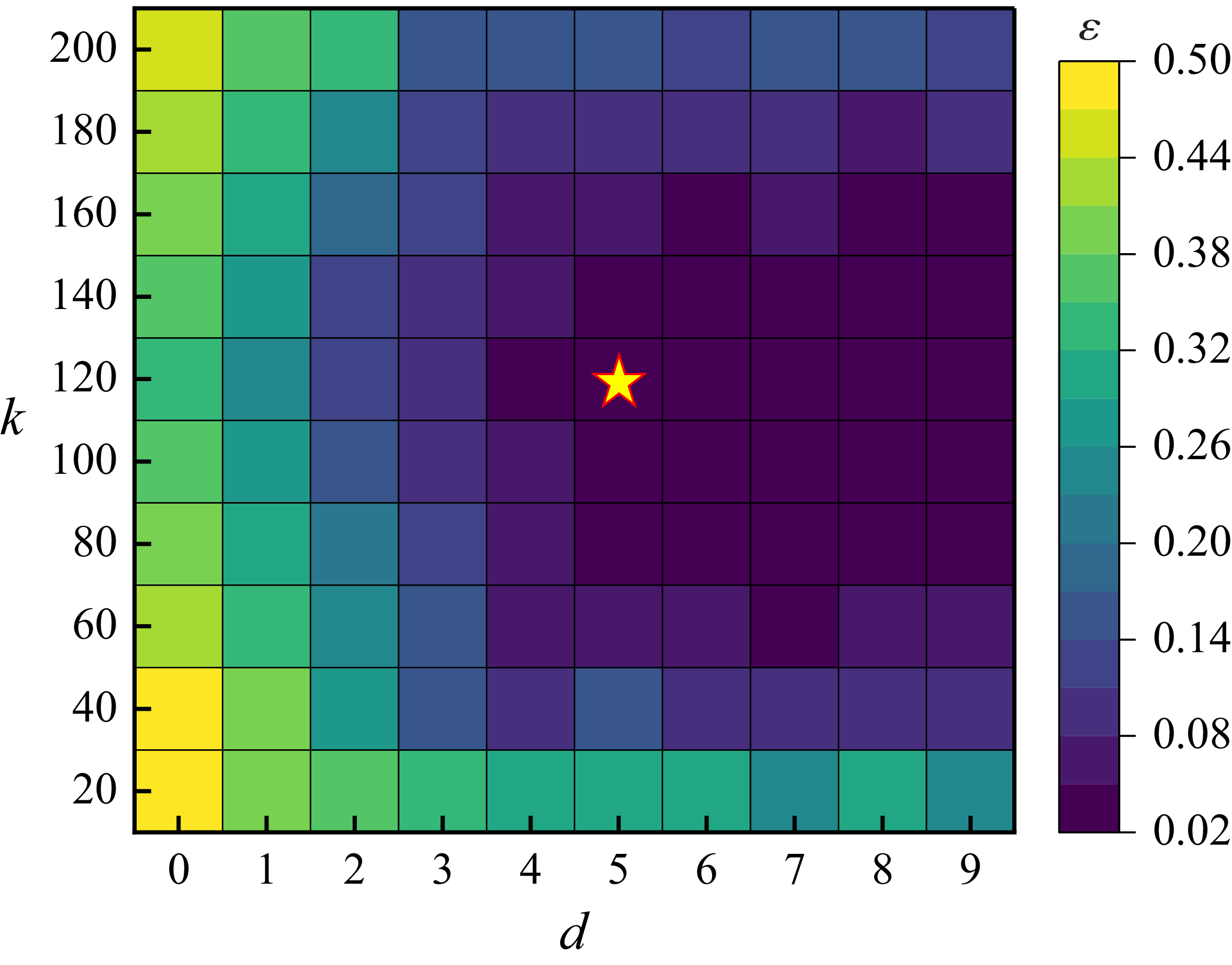
(a) Relative error
 $\varepsilon$
as a function of time-delay embedding order
 $d$
and the ROM rank
 $k$
. The yellow star at
 $(d,k) = (5,140)$
represents the parameters used in this study.

The rank
 $k$
of the Koopman ROM and the delay embedding dimension
 $d$
are the two most influential parameters governing ROM accuracy. Figure 8 presents a contour map illustrating how the ROM error
 $\varepsilon$
varies across delay embedding dimensions
 $d \in [0,9]$
and ROM ranks
 $k\in [20,200]$
. We first establish the necessity and effectiveness of delay embedding when using sparse measurements by fixing
 $k = 120$
. Without delay embedding (
 $d = 0$
), the ROM error remains substantially high (i.e.
 $\varepsilon = 0.32$
). As delay embedding is introduced, ROM accuracy improves markedly, with error decreasing rapidly as
 $d$
increases for
 $0\lt d \leq 4$
. For
 $d\gt 4$
, the error
 $\varepsilon$
shows little further reduction across all
 $k$
, confirming the effectiveness of moderate delay embedding under sparse measurements.
Similarly, we fix
 $d=5$
and examine how the ROM error varies with model rank
 $k$
. Interestingly, the results reveal a non-monotonic trend: increasing ranks does not necessarily yield better accuracy. This is attributed to the inclusion of spurious modes at higher ranks (as illustrated in figure 7), which may degrade the performance of the ROM. In this study we construct the Koopman ROM using
 $k = 120$
and
 $d = 5$
(marked by an asterisk), yielding a reconstruction error
 $\varepsilon$
below 0.03. This choice offers a balanced trade-off between model accuracy and computational cost, as further increases in embedding dimension lead to considerable overhead without significant improvement in performance.
Comparison between the true and reconstructed displacement responses at three probe locations. The top row (ai–ci) shows the results for (a) the LAF case with
 $\bar {u}_1 = 0.3$
, (b) the SDF case with
 $\bar {u}_3 = 0$
, and (c) the SAF case with
 $\bar {u}_5 = -0.3$
. The bottom row (aii–cii) presents the corresponding relative error for each probe.

Based on the selected modelling parameters, we construct Koopman ROMs for each combination of flapping mode (LAF, SDF, SAF) and control input level (
 $\bar {u}_1$
to
 $\bar {u}_5$
), resulting in a total of 15 autonomous systems. Figure 9 presents representative comparisons between the reconstructed displacement
 $\delta (t)$
with the full-order results within the range
 $t \in [0, 1.5]$
for three selected cases: the LAF case with
 $\mathcal{K}_{\bar {u}_1}$
, the SDF case with
 $\mathcal{K}_{\bar {u}_3}$
and the SAF case with
 $\mathcal{K}_{\bar {u}_5}$
. As shown in figure 9(ai–ci), the Koopman ROMs closely match the reference displacements at all three probe locations, especially in capturing the local peaks. Figure 9(aii–cii) displays the real-time relative error
 $(\delta _t - \delta _r)/\delta _m$
, where
 $\delta _m$
is the maximum displacement across the three probes in
 $t \in [0,1.5]$
. As expected for Koopman-based models, the reconstruction error increases with time. Therefore, we set the prediction horizon to
 $t_p = 1.0$
to ensure prediction accuracy within MPC, which is approximately one-fifth of the oscillation period. Within this range, the ROM maintains an average error below 5 %, which proves sufficient for effective closed-loop control. In our framework, each control cycle begins with the probes measuring the current system state
 $\boldsymbol{\delta }$
. This measurement serves as the initial condition for the Koopman ROMs, which then predicts the system’s future dynamics over a prediction horizon
 $t_p$
. An optimal control sequence is computed based on this prediction, but only the initial control action is executed on the full-order FSI system over a single control time step
 $t_c$
. This iterative loop continues throughout the control duration.
Time evolution of the displacement response
 $\delta$
at the trailing edge of the plate (ai–ci) and the corresponding control input
 $u$
(aii–cii) for the (a) LAF, (b) SDF and (c) SAF cases. Control is activated at
 $t = 300$
(red dashed line), after the system reaches a fully developed state (grey shaded region). The five time instants
 $t_1 = 302$
,
 $t_2 = 310$
,
 $t_3 = 320$
,
 $t_4 = 330$
and
 $t_5 = 360$
(marked by yellow diamonds) are selected for detailed visualisation in figure 11.

3.3. Suppressing the plate’s flapping by ROM-MPC controller
Next, we apply the established Koopman ROM to control the full-order fluid–structure coupled system across all three vibration modes (LAF, SDF and SAF). The control objective is to suppress the flapping motion and stabilise the flap to an undeformed equilibrium state, i.e.
 $\boldsymbol{\delta }_{\textit{ref}} = 0$
. The control input
 $u$
is obtained by solving the optimisation problem (2.37), and it is updated every
 $t_c = 0.2$
control horizon, approximately one twenty-fifth of the oscillation period. Figure 10 presents the time evolution of response
 $\delta$
and control input
 $u$
before and after control activation for the LAF, SDF and SAF cases. The control is activated at
 $t = 300$
, by which time the flow has entered a fully developed state, i.e. exhibiting limit-cycle periodic motion. Notably, the control algorithm exhibits strong robustness to varying initial conditions, consistently achieving successful suppression. For the LAF case (figure 10
ai), the uncontrolled displacement amplitude is
 $\delta _{\textit{amp}} = 0.41$
. After activating control,
 $\delta$
undergoes a slight amplification cycle, reaching a maximum value of 0.45 before beginning to decay. This transient increase is attributed to the strong actuation injecting additional disturbance energy into the system, reshaping the mean flow field structure and thereby stimulating non-modal energy amplification. Similar responses have been reported in previous studies on jet control strategies (Li & Zhang Reference Li and Zhang2022; Jiang & Cao Reference Jiang and Cao2024). Figure 10(aii) shows the control input
 $u$
, which reaches its maximum value during the initial few cycles and gradually decreases as the plate’s oscillation decreases. Furthermore, we find that the dominant flapping frequency after control closely matches the frequency identified in the resolvent analysis, consistent with findings in Gross et al. (Reference Gross, Marks and Sondergaard2024). This suggests that resolvent analysis can also offer valuable guidance for controlling FSI systems. To visualise the control effect more intuitively, figure 11 presents flow snapshots at five representative time instants (
 $t_1$
–
 $t_5$
) during the control process. As shown in figure 11(ai–aiii), the blowing–suction actuators continuously modify the vortex structures above and below the plate, progressively altering the vorticity field and adjusting the plate’s deformation accordingly. The ‘2S’ vortex shedding mode is gradually suppressed from
 $t_1$
to
 $t_3$
, with vortices becoming narrower and more aligned with the flow direction. Simultaneously, the plate undergoes different deformation states under fluid loading. By
 $t_4$
and
 $t_5$
, the original ‘2S’ vortex shedding mode has been effectively suppressed, and the flow field evolves toward a more streamlined configuration with reduced and evenly distributed vorticity. The entire system exhibits an undeformed equilibrium state. For the SDF case, the uncontrolled plate exhibits biased flapping, with its displacement significantly deviating from the target equilibrium position (figure 10
bi). When the control is applied, the asymmetric blowing-suction jets (figure 10
bii) disrupt the original oscillation mode (figure 11
bi). After
 $t \gt 305$
, the plate crosses into the
 $\delta \gt 0$
region and undergoes another amplification cycle. Figure 11(bii–biii) shows that during this phase, the flow field becomes more unstable and begins to develop the ‘2S’ separated vortices. After
 $t \gt 320$
, the flow field enters an oscillation decay phase (figure 11
biv), with both plate displacement and control input
 $u$
returning to a symmetric oscillatory state. By
 $t \gt 330$
, the plate reaches an unbiased equilibrium, successfully achieving the control objective. The control behaviour in the SAF case resembles that of the LAF case. As shown in figure 10(c), the system exhibits symmetric decay of plate oscillations under control. The corresponding flow field snapshots in figure 11(c) further confirm this trend, showing a monotonic suppression of vortex shedding and flow stabilisation.
Five snapshots of vorticity contours during control: (a) LAF case, (b) SDF case and (c) SAF case corresponding to figure 10.

To illustrate the evolution of coherent flow structures and stability characteristics before and after control, we perform Koopman modal analysis for the three flapping cases. To extract Koopman modes, we collect 500 flow field snapshots at a time interval of
 $\Delta t = 0.1$
over
 $t = 300$
–
 $350$
. Reduced-order modelling using the full state of the flow field can achieve high accuracy without the need for time-delay embedding
 $(d=0)$
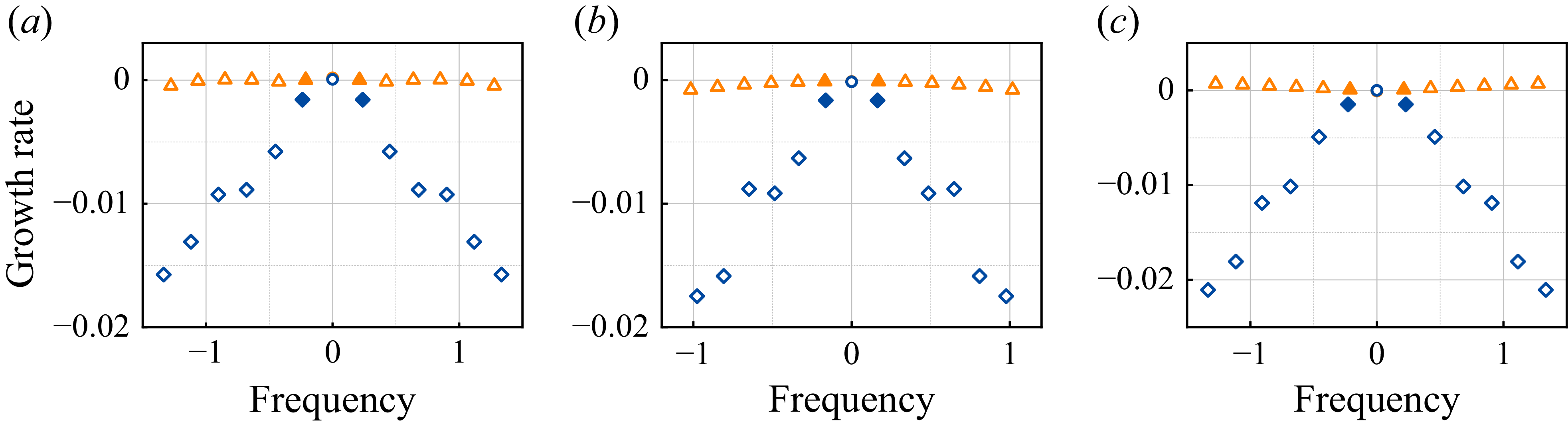
(Colbrook et al. Reference Colbrook, Ayton and Szőke2023). A comparison between the reconstructed flow field and the ground truth reveals that the average error is less than 1 %. Figure 12(a–c) presents the first 13 eigenvalues (frequency
 $f = \lambda _r /2\pi$
and growth rate
 $\lambda _i$
, sorted by residuals) before and after control. For all three cases, the leading four modes exhibit growth rates of the order of
 $\mathcal{O}(10^{-3})$
or smaller, indicating that these modes are neutrally stable. Here
 $M_0$
is the mean mode with
 $f = 0$
and the
 $M_1$
mode corresponds to the dominant oscillation frequency. It can be seen that, after control is applied, the eigenvalue distribution changes significantly: except the mean mode
 $M_0$
, all other modes exhibit increased decay rates and changing frequencies. As shown in figure 12(a), for the LAF case, the eigenvalue of
 $M_1$
shifts from
 $(\lambda _r/2\pi , \lambda _i) = (0.212, 1.83 \times 10^{-5})$
to
 $ (0.238, -1.58 \times 10^{-3})$
. Similar trends are observed for the SDF and SAF cases.
Distribution of the leading 13 Koopman eigenvalues before (orange triangles) and after (blue rhombi) control for the (a) LAF, (b) SDF and (c) SAF cases. The hollow circles represent the mean mode
 $M_0$
and the filled markers denote the dominant oscillation mode
 $M_1$
.

Comparison of key Koopman modes for the uncontrolled and controlled systems. The columns correspond to the (a) LAF, (b) SDF and (c) SAF cases. The top two rows visualise the mean flow mode (
 $M_0$
), while the bottom two rows visualise the dominant oscillatory mode (
 $M_1$
). For each mode, the figure compares the uncontrolled case (rows 1 and 3) with the corresponding controlled case (rows 2 and 4). The dashed boxes in (ai) indicate three streamwise regions: R1 (
 $0.5 \lt x \leqslant 2.5$
), R2 (
 $2.5 \lt x \leqslant 6$
) and R3 (
 $6\lt x \leqslant 13$
).

We focus on analysing the characteristics of the mean mode
 $M_0$
and the dominant oscillation mode
 $M_1$
. The first two rows of figure 13 illustrate the spatial distribution of
 $M_0$
for the LAF, SDF and SAF cases under both uncontrolled and controlled conditions. The downstream region is partitioned into three distinct zones: R1 (the immediate wake encompassing the plate,
 $0.5 \lt x \leqslant 2.5$
), R2 (the intermediate wake,
 $2.5 \lt x \leqslant 6$
) and R3 (the far wake,
 $6 \lt x \leqslant 13$
). Vortices are generated in R1, amplified in R2 and subsequently advected into the far-field region R3. In the LAF case (figures 13
ai and 13
aii), the mean mode undergoes significant alterations across all three regions after control is applied. Post-control, the vorticity becomes more concentrated near the flexible plate in the latter part of region R1 (
 $1.5 \lt x \leqslant 2.5$
). Furthermore, a symmetric and elongated shear layer emerges in regions R2 and R3. This phenomenon occurs because the control suppresses both the flapping motion and vortex shedding. Conversely, for the SDF case, region R1 shows minimal change between the uncontrolled and controlled states (figures 13
bi and 13
bii). In contrast, regions R2 and R3 exhibit an opposite trend compared with the LAF case: a shear layer prominent in the uncontrolled flow vanishes after control is activated. This is because the control action transiently disrupts the deflected state, compelling the system to transition towards a symmetric configuration. The SAF case (figures 13
ci and 13
cii) is analogous to the LAF case, but the post-control shear layer in regions R2 and R3 is wider than that observed in the controlled LAF case (figure 13
aii). Collectively, this comparison demonstrates that the application of control induces significant structural changes in the
 $M_0$
mode, confirming that the proposed strategy fundamentally alters the time-averaged characteristics of the flow field.
Next, we analyse the dominant oscillation mode
 $M_1$
. For the LAF case, figures 13(a
iii) and 13(aiv) show that before and after control, the morphological characteristics of the vorticity in the three regions remain almost unchanged, but there are some changes in amplitude. The mode amplitude in the latter half of region R2 and in region R3 is lower than before control, indicating that the shear and separation effects of the plate are weakened during the control process. For the SAF case, as shown in figures 13(ciii) and 13(civ), the dominant vortex pattern exhibits noticeable changes mainly within region R1, reflecting the effect of jet actuation on near-wall travelling waves. We observe that the modifications of
 $M_1$
in these two cases are relatively minor compared with the SDF case. Figures 13(b
iii) and (biv) show the SDF case. Before the control, the dominant vorticity within
 $M_1$
mode is primarily concentrated in R2 and R3, exhibiting a typical Kármán vortex street resembling that of a pure fluid system. After control is applied, the
 $M_1$
mode undergoes significant changes in all three regions. Specifically, the vorticity increases markedly in R1, while the vortex patterns in R2 and R3 become broader and more irregular compared with the uncontrolled case. In our previous work on using balanced proper orthogonal decomposition (BPOD)-ROM for cylinder VIV control (Jiang & Cao Reference Jiang and Cao2024), we found that control either modified existing modes or created new ones, and additional energy is required to sustain the newly induced modes. A similar pattern appears here: for LAF and SAF, the Koopman-based control alters the original mode
 $M_1$
, while for SDF, it generates a new dominant mode.
We further analyse the control mechanism from an energy transfer perspective. For the present FSI system, we calculate the energy variations of the plate and the flow field kinetic energy relative to the undeformed equilibrium state during the control process, as well as the energy injected into the flow field by actuators. First, for the Saint-Venant–Kirchhoff material, the elastic potential energy and kinetic energy densities can be calculated as
 \begin{equation} {{w}_{p}}=\frac {{{\lambda }_{s}}}{2}{{\left \{ {tr}\left [ \boldsymbol{E}({{\eta }_{s}}) \right ] \right \}}^{2}}+{{\mu }_{s}}{\textit{tr}}\big [\boldsymbol{E}{{({{\eta }_{s}})}^{2}} \big ], \qquad w_k = \frac {M}{2}\left (\frac {{\textrm d} \eta _{s}}{{\textrm d}t} \right )^2\!, \end{equation}
where
 $w_p$
is the elastic potential energy density and
 $w_k$
is the kinetic energy density. Total energy variations for structure and flow field are
 \begin{equation} W_s = \int _{\varOmega _s} (w_p + w_k) {\textrm d}\varOmega - \int _{\varOmega _s} \bar {w}_p {\textrm d}\varOmega , \qquad W_{\kern-1pt f} = \int _{\varOmega _f} \frac {\boldsymbol{u}^2}{2} {\textrm d}\varOmega -\int _{\varOmega _f} \frac {{U}^2}{2} {\textrm d}\varOmega , \end{equation}
where
 $\bar {w}_p$
and
 $U$
represent the UE state. Furthermore, energy injected into the flow field by the jet for
 $t_0$
–
 $t_e$
are
 \begin{equation} W_i = \int _{t_0}^{t_e} \left \{\int _{\varGamma _{\!j}} \frac {\left [{Q_{t} h(\boldsymbol{u}_{\!j})}\right ]^2}{2} {\textrm d}x\right \} {\textrm d}t, \end{equation}
where
 $\varGamma _{\!j}$
is the surface of the jet on the cylinder,
 $h(\boldsymbol{u}_{\!j})$
represents the jet velocity profile and
 $Q_t$
is the time-varying magnitude of the jet. We define two energy metrics: the cumulative injected energy,
 $W_i^t$
, which is the total kinetic energy injected from a fixed start time
 $t_0 = 300$
to the current time
 $t_e = t$
; and the single-injected energy,
 $W_i^p$
, representing the kinetic energy from a single jetting action over a sliding time window of fixed duration
 $t_c$
(where
 $t_e - t_0 = t_c$
).
(a) Evolution of cumulative jet energy
 $W^t_i$
and total flow field energy
 $(W_{\kern-1pt f} + W_s)$
from
 $t = 300$
to
 $400$
for the LAF, SDF and SAF cases, with colour indicating temporal progression. Panels (b), (c) and (d) show time evolution of the actuation jet energy
 $W^p_i$
for the LAF, SDF and SAF cases, respectively.

Figure 14(a) illustrates the relationship between the accumulated jet energy
 $W_i^t$
from actuators and the flow field energy (
 $W_s + W_{\kern-1pt f}$
) over time. There exists a time delay between the initial application of control and its effectiveness. For the LAF case, during the initial control phase (
 $300 \lt t \lt 330$
), the flow field energy maintains a magnitude comparable to the uncontrolled state. When
 $330 \lt t \lt 360$
, the control effect begins to manifest as
 $W_s + W_{\kern-1pt f}$
decreases linearly with an approximate slope of
 $-1510$
, and
 $W_i^t$
falls within the range
 $[1.4, 1.8]$
. When
 $t \gt 360$
, the flow field energy continues to decline, while the jet energy approaches a limiting value with minimal temporal variation,
 $W_i^t \rightarrow 1.81$
. Similar behaviour is observed in the SAF case, with the key distinction being that a higher final jet energy expenditure of
 $W_i^t \rightarrow 2.2$
is required to achieve significant attenuation. For the SDF case,
 $W_s + W_{\kern-1pt f}$
initially maintains the smallest magnitude compared with the other two cases. When
 $2 \lt W_i^t \lt 2.3$
, the flow field energy begins to increase rapidly before experiencing substantial linear decay. We find that the SDF case requires the highest total jet energy of
 $W_i^t \rightarrow 2.75$
to completely suppress instability. Figures 14(b), 14(c) and 14(d) illustrate the time evolution of
 $W_i^p$
for each jetting action after time
 $t \gt 350$
. It can be observed that the jetting energy maintains a small magnitude during this period. This is because all three cases have reached a stable equilibrium state accompanied by very weak flapping, as shown in figure 10. Consequently,
 $W_i^p$
also gradually decays as the flapping motion attenuates. The role of the controller at this stage is to maintain this stable state and prevent the re-emergence of LAF triggered by the inherent instability of the FSI system. Based on the modal decomposition results presented above, flow control in the SDF case operates by generating new modes that consume more energy, while the LAF and SAF cases modify the original inherent modes, consuming less energy. This conclusion aligns with the findings of Jiang & Cao (Reference Jiang and Cao2024).
Time evolution of elastic potential energy
 $W_p$
and kinetic energy
 $W_k$
of the plate in a range of
 $t \in [290,330]$
for the (a) LAF case, (b) SDF case and (c) SAF case.

(a) Time evolution of
 $W_p$
,
 $W_k$
and
 $W_s$
from
 $t = 296$
to 310 for the SDF case. (b) Leading instability eigenmode calculated by global linear instability analysis. (c)-(h) Snapshots of the flow field at six representative time instances (
 $t_1$
–
 $t_6$
). Here
 $V^+$
and
 $V^-$
denote vortices rotating in the counterclockwise and clockwise direction, respectively.

To better understand the plate’s energy evolution during control, figure 15 presents the time history of elastic potential energy
 $W_p$
and kinetic energy
 $W_k$
. For the LAF case, the plate’s low Young’s modulus leads to relatively small elastic potential energy
 $W_p$
, approximately one-tenth of
 $W_k$
. Consequently, the plate’s energy is predominantly governed by its kinetic component as shown in figure 15(a). After control is applied, both
 $W_p$
and
 $W_k$
increase with time until
 $t \lt 308$
, with the increase in kinetic energy significantly exceeding that of potential energy. For the SDF case, the plate initially exhibits a biased flapping state with increased stiffness, storing unreleased elastic potential energy around
 $W_p = 4$
(figure 15
b). Due to the limited flapping amplitude, the kinetic energy remains low at
 $W_k = 0.2$
. Once control is applied, however,
 $W_k$
increases significantly, peaking at 20. For the SAF case, we observe that
 $W_p$
and
 $W_k$
exhibit nearly identical amplitudes but opposite phases, as shown in figure 15(c). This indicates a cyclical process where kinetic energy converts to potential energy, which subsequently releases and transforms back into kinetic energy. Moreover, we define energy efficiency as the ratio of the dissipated mechanical energy of the structure (the sum of its kinetic and potential energy) to the cumulative energy
 $W_i^t$
injected by the jets. It is found that our control strategy has a high energy efficiency.
Figure 16(a) shows the time evolution of elastic potential and kinetic energy from
 $t = 296$
–
 $310$
for the SDF case. At
 $t = t_1$
, the jet actuation induces vortex
 $V_1^+$
, which is initially locked at the junction between the cylinder’s lower right side and the plate, enhancing its intensity and advects it downstream. Figure 16(b) illustrates the plate’s transition from equilibrium to deflected state through a ‘symmetry-breaking’ mechanism, which explains the presence of the locked vortex
 $V_1^+$
as evidenced in figure 5(c). By
 $t = t_2$
, vortex
 $V_1^+$
has reached the plate’s trailing edge and escaped the previously confining region shown in figure 16(d). During this process, both
 $W_p$
and
 $W_k$
increase simultaneously as the plate oscillates downward. At
 $t = t_3$
, the plate reaches maximum deflection with
 $W_p = 6$
and a new vortex
 $V_2^+$
forms (figure 16
e). As the plate reverses direction, upper-side vortices are shed into the flow, completing one cycle (figure 16
f). At
 $t = t_4$
, the plate’s elastic potential energy begins to release while its kinetic energy increases, establishing a phase difference between
 $W_p$
and
 $W_k$
. With the original biased oscillation being disrupted, the plate enters the
 $y \gt 0$
region, and the shedding dynamics begin to resemble those of the SAF case. Figures 16(g) and 16(h) illustrate the alternating vortex shedding process corresponding to times
 $t_4$
and
 $t_5$
in figure 16(a). This sequence reveals the ‘breaking’ control mechanism that the actuation exerts on the SDF solution. Specifically, the control effectively disrupts the locked vortex structure that maintains the deflected state, thereby initiating a transition toward a more symmetric flapping pattern characterised by alternating vortex shedding.
(a) An illustration of the RL framework. (b) Training process for the LAF case. Testing process: (c) time evolution of the displacement response
 $\delta$
and (d) the corresponding control input
 $u$
.

Having established the effectiveness of the Koopman-MPC, we now turn to its computational efficiency, particularly in comparison to RL approaches. We compare the computational efficiency of our method with RL approaches. In both frameworks, the most time-consuming component lies in the use of full-order FSI simulations: in our method, full-order simulation results are used to train Koopman ROMs, while in RL, they provide the simulation environment for agent training. Therefore, we compare the two methods by evaluating the amount of full-order simulation time required to derive effective control strategies. For a fair comparison, all computations in the present study were performed on an Intel(R) Xeon(R) Silver 4216 processor (32 cores @ 2.1 GHz). Further details regarding the RL framework implementation and Koopman ROM training can be found in Appendix C. For the LAF case, the training results under the RL framework of figure 17(a) are shown in figure 17(b). The proximal policy optimisation (PPO) agent typically learns the control strategy after approximately 120 episodes, requiring about 125 hours, significantly exceeding the training time of the Koopman ROM (10.5 h). Regarding the control performance, the RL controller begins by applying a stronger actuation, as shown in figure 17(d). This aggressive initial action causes a transient increase in displacement (figure 17
c) but achieves a more rapid initial amplitude decay compared with the ROM-based method. However, the decay rate slows in the later stages, resulting in a total control time comparable to the ROM method for a stricter objective, such as
 $\delta \lt 0.05$
. These results highlight the computational efficiency of the proposed Koopman-based approach. Nevertheless, this does not suggest that it can fully replace RL methods, especially as recent advances have greatly improved the data efficiency of RL algorithms (Liu & MacArt Reference Liu and MacArt2024; Jia & Xu Reference Jia and Xu2024).
4. Conclusions
This paper presents a switched-system relaxation control framework for FSI systems by integrating a Koopman-based ROM with MPC algorithms. The control objective is to suppress the instability of a flexible plate in the wake of a cylinder by regulating blowing-suction jet actuators mounted on the cylinder. We begin by analysing the fluid dynamics of the uncontrolled system at fixed parameters:
 $\textit{Re} = 150$
,
 $M_s = 1$
,
 $v_s = 0.35$
, while varying only the Young’s modulus
 $E_s$
. Within the range
 $2\times 10^4 \leqslant E_s \leqslant 6\times 10^6$
, three characteristic dynamic regimes are observed as
 $E_s$
increases: LAF, SDF and SAF. To achieve active control for these three fluid–structure coupling instability cases, we select
 $E_s=4\times 10^4$
(LAF),
 $4\times 10^5$
(SDF) and
 $4\times 10^6$
(SAF) as representative cases for comparative studies.
Prior to developing the Koopman ROM and active control strategy, we implement resolvent analysis applicable to global elastic fluid–structure coupling systems to determine the optimal actuator and probe placement. The optimal forcing mode
 $\hat {\boldsymbol{f}}_1$
guides the placement of actuators. Specifically, the mode reveals that high forcing magnitudes primarily concentrate at the cylinder’s trailing edge and the plate’s leading edge across all three cases. By calculating the energy density
 $k_{\theta }$
of the forcing mode near the cylinder, we identify an averaged high
 $k_{\theta }$
region within
 $\theta \in [60^{\circ },70^{\circ }]$
. Accordingly, we place actuators symmetrically along the
 $x$
axis within this interval, aligning with the vortex shedding separation points of the cylinder and enabling effective jet manipulation of vortex shedding for fluid–structure coupling control. Subsequently, the optimal response mode
 $\hat {\boldsymbol{\eta }}_1$
informs the probe placement strategy. Unlike traditional flow field-based probe placement, our approach locates probes directly on the flexible structure, aligning better with practical engineering constraints. Through careful selection of three key measurement locations (
 ${P}_1(x = 1.4)$
,
 ${P}_2(x = 1.9)$
and
 ${P}_3(x = 2.4)$
), we effectively capture the dynamic characteristics of the severe oscillation regions in the posterior section of the structure. Despite the modelling challenges introduced by sparse sensing, our Koopman-based ROM maintains high accuracy, successfully addressing the difficulties in system observability and potential degradation in model fidelity. This unified actuator–probe configuration strategy significantly simplifies the complexity of control system design, providing a practical and efficient solution for fluid–structure coupling control in complex engineering environments.
Then, we investigate Koopman-based reduced-order modelling and examine the influence of the delay embedding dimension
 $d$
and model order
 $k$
on model accuracy. Initially, we construct the preliminary Koopman ROM using the KDMD algorithm. To improve accuracy, the ResDMD algorithm is employed to identify and eliminate spurious modes. After balancing model fidelity and computational cost, we select
 $(k,d)=(120,5)$
for the reduced-order modelling process. Under this pair of parameters, our Koopman ROM achieves high reconstruction accuracy, with a relative error below 5 % over a prediction horizon
 $t_p=1$
(i.e. approximately one-fifth of the oscillation period). The trained Koopman ROMs are then integrated into a MPC framework to control the full-order FSI system. Separate ROMs are constructed for the LAF, SDF and SAF cases. We successfully achieve active control for all three cases, effectively suppressing the plate’s flapping motion (
 $\boldsymbol{\delta }^{\textit{ref}} = 0$
). During the stabilisation phase, both plate displacement and control input attenuate over time, and the output frequency of control
 $u$
aligns with the prediction from resolvent analysis.
We employ Koopman modal decomposition to investigate how the Koopman-MPC controller achieves active flow–structure interaction control through modal regulation. In all three cases, after the control is activated, the growth rates of the dominant Koopman eigenvalues shift into the stable region (
 $\lambda _i \lt 0$
), accompanied by changes of frequencies. For the principal mode
 $M_1$
, the spatial structures in LAF and SAF cases exhibit minimal changes, with only localised modifications. In contrast, the SDF case exhibits a qualitatively new mode that disrupts the original Kármán vortex street, producing broader and more irregular flow–structure interaction features. To quantify control effort, we calculate the evolution of structural energy
 $W_s$
, fluid energy
 $W_{\kern-1pt f}$
and cumulative jet energy
 $W_i^t$
during the control process. Among the three cases, the SDF case consumes the most jet energy (
 $W_i^t = 2.75$
) to form the new mode, whereas the LAF and SAF cases achieve control by modifying inherent modes, requiring only
 $W_i^t = 1.81$
and
 $2.20$
, respectively. This observation aligned with our previous BPOD-based cylinder VIV control study (Jiang & Cao Reference Jiang and Cao2024). Additionally, by combining vortex dynamics with energy analysis, we find that the successful control in the SDF case can be attributed to the disruption of the original ‘symmetry-breaking’ mechanism, allowing trapped vortices between the cylinder and plate to be released. Finally, comparison with RL methods highlights the superior computational efficiency of our approach, demonstrating not only effective control performance but also practical feasibility for real-world fluid–structure problems.
Funding
This work was supported by the National Key R&D Program of China (Grant No. 2024YFC3013200) and the Shenzhen Peacock Plan (Grant No. QD2023006C).
Declaration of interests
The authors report no conflict of interest.
Data availability statement
The code used in this work is made available at https://github.com/MFSI-Lab/Koopman-control-FSI.
Appendix A. Resolvent analysis
We conduct the resolvent analysis for the uncontrol FSI system, i.e. autonomous systems without control. In resolvent analysis the governing equation is first established, i.e.
 \begin{equation} \frac {\partial \boldsymbol{x}}{\partial t} = \boldsymbol{R}[\boldsymbol{x}( t)]. \end{equation}
Considering the Reynolds decomposition of the flow variables
 $\boldsymbol{x}( t) = {X} + \boldsymbol{x}^{\prime}( t)$
, where
 $X$
is base flow and
 $\boldsymbol{x}^{\prime}(t)$
is the perturbation of the flow field. Substituting the Reynolds decomposition into (A1), a forced linearised dynamical system can be obtained, i.e.
 \begin{equation} \frac {\partial \boldsymbol{x}^{\prime}}{\partial t} = \boldsymbol{L}\boldsymbol{x}^{\prime} + \boldsymbol{f}^{\prime}, \end{equation}
where
 $\boldsymbol{L}$
is the linearised operator of the governing equations; details of the linearisation of the nonlinear FSI system are shown in Appendix D. In the linear framework we assume a harmonic forcing
 \begin{equation} \boldsymbol{f}^{\prime}(t) = \hat {\boldsymbol{f}}{\textrm e}^{{\rm i}\omega t} + \textrm{c.c.}, \end{equation}
where
 $\textrm{c.c.}$
stands for the complex conjugate. Because of the linearity of (A2), this harmonic forcing leads to a harmonic fluid response
 \begin{equation} \boldsymbol{x}^{\prime}(t) = \hat {\boldsymbol{x}}{\textrm e}^{{\rm i}\omega t} + \textrm{c.c.}, \end{equation}
where the state
 $\hat {\boldsymbol{x}}$
represents a fluid–structure mode. Introducing the matrix approximation of the resolvent operator
 $\boldsymbol{H} ( \omega )={{ ( {\rm i}\omega {\boldsymbol{I}}-{\boldsymbol{L}} )}^{-1}}$
, the response
 ${\hat {\boldsymbol{x}}}$
to a forcing
 $\hat {\boldsymbol{f}}$
is
 \begin{equation} {{\hat {\boldsymbol{x}}}}=\boldsymbol{H}( \omega)\hat {\boldsymbol{f}}. \end{equation}
Before further discussing the resolvent analysis, we need to introduce several definitions of energy. We calculate the energy variations of the plate and the flow field kinetic energy. For the Saint-Venant–Kirchhoff material, the elastic potential energy and kinetic energy densities can be calculated as
 \begin{equation} {\hat {w}_{p}}=\frac {{{\lambda }_{s}}}{2}{{\left \{ {\textit{tr}} \!\left [ \boldsymbol{E}({\hat {\eta }_{s}}) \right ] \right \}}^{2}}+{{\mu }_{s}}{\textit{tr}} \big [\boldsymbol{E}{{({\hat {\eta }_{s}})}^{2}} \big ], \quad \hat {w}_k = \frac {M}{2}\left (\frac {{\textrm d} \hat {\eta }_{s}}{{\textrm d}t} \right )^2, \end{equation}
where
 $\hat {w}_p$
is the elastic potential energy density and
 $\hat {w}_k$
is the kinetic energy density. Total energy variations for the structure and flow field are
 \begin{equation} \hat {W}_s = \int _{\varOmega _s} (\hat {w}_p + \hat {w}_k){\rm d}\varOmega , \quad \hat {W}_{\kern-1pt f} = \int _{\varOmega _f} \frac {\hat {\boldsymbol{u}}^2}{2} {\rm d}\varOmega . \end{equation}
Then, in order to study the amplification of the FSI system subjected to harmonic forcings with different frequencies, we define two physically relevant norms of the state vector as
 \begin{equation} \big\| \hat {\boldsymbol{f}} \big\|^2_{ \boldsymbol{Q}_{\!f}} = \hat {\boldsymbol{f}}^{\dagger } \boldsymbol{Q}_{\!f} \hat {\boldsymbol{f}}, \quad \left \| \hat {\boldsymbol{q}}_r \right \|^2_{ \boldsymbol{Q}_{u}} = \hat {\boldsymbol{q}}_r^{\dagger } \boldsymbol{Q}_{u} \hat {\boldsymbol{q}}_r, \end{equation}
where
 $\dagger$
represents the Hermitian transpose and
 $\hat {\boldsymbol{q}}_r = ({\hat {\boldsymbol{u}}}, \hat {\eta }_{s}, \dot {\hat {\eta }}_s)$
. The matrices
 $\boldsymbol{Q}_{\!f}$
and
 $\boldsymbol{Q}_{u}$
correspond to the discrete operators used to compute the spatial norms over the fluid computational domain, i.e.
 \begin{equation} {\boldsymbol{Q}_{\!f}} = \begin{bmatrix} \boldsymbol{L}_{\kern-1pt f}^{2n_a} & \boldsymbol{0} \\ \boldsymbol{0} & \boldsymbol{L}_{\kern-1pt f}^{2n_b} \end{bmatrix}, \quad {\boldsymbol{Q}_{u}} = \begin{bmatrix} \boldsymbol{L}_{\kern-1pt f}^{2n_t} & \boldsymbol{0} & \boldsymbol{0} \\ \boldsymbol{0} & \boldsymbol{L}_p^{2n_s} & \boldsymbol{0} \\ \boldsymbol{0} & \boldsymbol{0} & \boldsymbol{L}_k^{2n_s} \end{bmatrix}, \end{equation}
where
 $n_a$
and
 $n_b$
are the degrees of freedom for the fluid domain near the cylinder (
 $r \in [0.5,1.0]$
) and the remaining fluid domain, respectively. Here
 $n_t = n_a + n_b$
and
 $n_s$
represents the degrees of freedom for the structure. For the
 $\boldsymbol{Q}_f$
matrix, the components are
 $\boldsymbol{L}_{\kern-1pt f}^{2n_a} = \beta _f \boldsymbol{I}^{2n_a}$
and
 $\boldsymbol{L}_f^{2n_b} = \boldsymbol{0}^{2n_b}$
, where
 $\boldsymbol{I}$
and
 $\boldsymbol{0}$
are the identity and zero matrices, respectively. This formulation indicates that we only compute the jet kinetic energy in the region near the cylinder. For the
 $\boldsymbol{Q}_u$
matrix, the term
 $\boldsymbol{L}_f^{2n_t} = \beta _f \boldsymbol{I}^{2n_t}$
is used to compute the fluid kinetic energy, corresponding to
 $W_{\kern-1pt f}$
in (A7). Similarly, the matrices
 $\boldsymbol{L}_p^{2n_s} = \beta _p \boldsymbol{L}^{\prime}_p$
and
 $\boldsymbol{L}_k^{2n_s} = \beta _k \boldsymbol{I}^{2n_s}$
are defined to compute the potential and kinetic energy of the structure, corresponding to
 $\hat {W}_s$
in (A7), where
 $\hat {\eta }_{s}^{\dagger }\boldsymbol{L}^{\prime}_p \hat {\eta }_s$
is a calculation of
 $\hat {w}_p$
in (A6). Here
 $n_s$
is the degrees of freedom for the structure domain;
 $\beta _f$
,
 $\beta _p$
and
 $\beta _k$
are constants that incorporate the relevant physical parameters and scaling to approximate the integration involved in (A7). More details can be found in Goza & Colonius (Reference Goza and Colonius2018).
Then,
 $\sigma_1({\omega})$
can be quantified by the ratio of the physically relevant norm of the response to the forcing (Herrmann et al. (Reference Herrmann, Baddoo, Semaan, Brunton and McKeon2021)):
 \begin{equation} \sigma _{1}( \omega)=\underset {{{ \| \hat {\boldsymbol{f}} \|}^{2}_{\boldsymbol{Q}_{\!f}}}=1}{\mathop {\max }}\,{{\| {\hat {\boldsymbol{q}}_r} \|}^{2}_{\boldsymbol{Q}_{u}}}. \end{equation}
Using (A5) and the adjoint resolvent operator
 ${\boldsymbol{H}}{{ ( \omega )}^{\dagger }}$
, which corresponds numerically to the Hermitian transpose of
 ${\boldsymbol{H}} ( \omega )$
, the solutions to this constrained problem can be obtained by solving the generalised eigenvalue problem ( Brandt et al. (Reference Brandt, Sipp, Pralits and Marquet2011))
 \begin{equation} \big [ {\boldsymbol{H}}{{( \omega)}^{\dagger }}{\boldsymbol{Q}_{u}}{\boldsymbol{H}}( \omega) \big ]\hat {\boldsymbol{f}}={{\sigma }}{\boldsymbol{Q}_{\!f}}\hat {\boldsymbol{f}}. \end{equation}
The eigenvalues
 $\sigma _{1}\gt \sigma _{2}\gt \cdots$
are positive since the left- and right-hand sides of this problem are Hermitian. In the present case, the explicit form of the adjoint resolvent operator does not need to be determined and the discrete adjoint approach is considered. Once the forcing field is determined, the velocity perturbation response can by computed using (A5). The triplet
 $ [ {{\sigma }_{1}},{{ \hat {\boldsymbol{f}} }_{1}},{{ {{{\hat {\boldsymbol{q}}}}} }_{1}} ]$
is called optimal (gain, forcing, response) because the momentum forcing field
 ${ \hat {\boldsymbol{f}} }_{1}$
yields the most amplified velocity perturbation
 $\hat {\boldsymbol{u}}_{1}$
– by a factor according to the kinetic energy norm. The triplets
 $ [ {{\sigma }_{i}},{{ \hat {\boldsymbol{f}} }_{i}},{{ {{{\hat {\boldsymbol{q}}}}} }_{i}} ]$
are called suboptimum of order
 $i \gt 1$
, and represent less amplified couples of forcing and response, and we only consider the optimal case
 $i = 1$
. Note that these fields are given for each value of the forcing frequency: both the gain, the forcing and the response field depend on
 $\omega$
. A shift-and-invert Arnoldi method from the ARPACK library is used to solve the generalised eigenvalue problem (Lehoucq, Sorensen & Yang Reference Lehoucq, Sorensen and Yang1998; Jiang et al. Reference Jiang, Luo, Zhang, Wu and Yi2022; Luo et al. Reference Luo, Jiang, Wu, Zhang and Yi2023). The numerical method and verification of the linear/nonlinear numerical solutions are shown in Appendix E.
Contour of the base flow for the (a) LAF case and (b) SDF case.

Optimal energetic amplification for the LAF, SDF and SAF cases. The optimal energetic gain
 $\sigma _1$
is plotted as a function of the frequency
 $f = \omega /2\pi$
. The resolvent modes associated with the each peak
 $(f_1, f_2$
and
 $ f_3)$
are displayed in figure 20.

Appendix B. Resolvent-based actuator–probe placement
Resolvent analysis reveals high-gain regions in the flow, enabling strategic actuator and probe placement for efficient control with minimal energy input. In this section we present resolvent analysis conducted across three distinct FSI configurations – LAF, SAF and SDF – which reveals fundamental differences in their energy amplification characteristics and associated flow structures. The insights gained from this analysis inform our development of an optimised actuator–probe placement strategy that exploits the inherent dynamics of each system.
Figure 18 presents the base flow solutions for the LAF and SDF cases. The base flow for the SAF case is omitted as it is nearly identical to that of the LAF case. For the LAF configuration, figure 18(a) illustrates the spatial structure of the base flow, which is an undeformed equilibrium solution characterised by flow symmetry about the line
 $x = 0$
. In this state, the streamwise deformation of the elastic plate remains negligible, with a magnitude of the order of
 $O(10^{-3})$
. In contrast, for the SDF case, the base flow solution depicted in figure 18(b) represents a deflected equilibrium state where the symmetry is broken. This deflected equilibrium state is adopted as the base flow to facilitate a resolvent analysis of the transition from a deflected state to periodic flapping. Figure 19 presents the optimal energy gain curves
 $\sigma _1$
obtained by solving the eigenvalue problem (A11) for the three configurations. We investigate forcing frequencies within the range
 $0.1\leqslant f \leq 0.3$
. For the LAF case,
 $\sigma _1$
increases rapidly with
 $f$
, exhibiting an amplification peak at
 $\sigma _1(f_1 = 0.206) = 81\,254$
, indicating maximum perturbation amplification at this forcing frequency. For
 $f \gt f_1$
, the gain decreases monotonically with frequency up to the maximum frequency (
 $f = 0.3$
). Here, we focus solely on the peak condition; the spatial structures of the forcing
 $\hat {\boldsymbol{f}}$
and response fields
 $\hat {u}_x$
corresponding to the optimal gain peak are shown in figures 20(ai) and (a
ii). These figures display the real parts of the forcing and response fields, with their corresponding imaginary parts being similar but opposite in phase. The response (figure 20
a
ii) exhibits well-defined coherent structures extending downstream of the cylinder, characterised by alternating positive and negative velocity regions forming a highly organised vortex street, with amplitudes that increase in the downstream direction. The forcing is primarily concentrated in specific regions: near the cylinder and at the plate’s leading edge (figure 20
a
i), which forms elongated wave patterns that are angled relative to the direction of the flow. Its maximum amplitude is located upstream of the response, indicating that perturbations in these regions most efficiently excite the system’s primary response.
Contours of resolvent modes, showing the real part of the transverse velocity component. Panels (ai, aii) display the optimal forcing and corresponding response for the LAF case at
 $f_1$
marked in figure 19. Panels (bi, bii) and (ci, cii) show the respective results for the SDF and SAF cases at
 $f_2$
and
 $f_3$
, respectively.

In contrast, the SAF case exhibits a higher peak frequency of
 $f_3 = 0.216$
, but with a markedly lower gain of
 $\sigma _1 = 49\,225$
. The associated resolvent modes, shown in figures 20(c
i) and 20(c
ii), reveal similar spatial distributions to the LAF case, though with notable distinctions: the response mode features more compact structures with shorter wavelengths and the forcing mode is positioned closer to the cylinder-plate leading edge. Examining the gain curve in figure 19, the SDF case displays a pronounced peak at a lower frequency (
 $f_2 = 0.164$
), although with significantly reduced amplification compared with the LAF case. The spatial structure of its response mode resembles that of the LAF case, but with altered wavelength and reduced coherence, particularly in the near-wake region. This modification in modal structure likely results from the laterally mounted plate disrupting the natural formation of the Kármán vortex street, leading to the less efficient amplification peak observed in figure 19.
Based on the resolvent analysis presented above, we seek a unified optimal actuator–probe placement strategy by analysing the input resolvent modes in figure 20 to effectively control all three cases (LAF, SDF and SAF). Figure 21(a) shows the distribution of average kinetic energy density
 $k_{\theta }$
in the near-cylinder surface region
 $r= 0.5{-}0.55$
from
 $\theta = -180^\circ$
to
 $180^\circ$
, where
 $\theta =0^\circ$
corresponds to the rear stagnation point of the cylinder. The analysis reveals that the energy density
 $k_{\theta }$
for LAF and SAF exhibits two significant peaks at
 $\theta = \pm 76^\circ$
and
 $\theta = \pm 55^\circ$
, respectively, while the SDF case shows an asymmetric, broader distribution with peaks at
 $\theta = -66^\circ$
and
 $\theta = 63^\circ$
. Placing actuators at the peak regions of the forcing modes ensures maximal flow sensitivity and efficient energy transfer from input to output, enabling effective control with minimal actuation effort. Based on the averaged
 $k_{\theta }$
profiles across all three cases, we employ a universal placement strategy of the blowing-suction actuator within the purple shaded region in figure 21(a), spanning approximately from
 $\theta _1 =60^\circ$
to
 $\theta _2 = 70^\circ$
on both sides of the cylinder, with
 $\Delta w = 10^\circ$
(figure 22
a). Notably, the chosen actuator positions coincide with flow separation points, allowing effective influence on the vortex shedding process, thereby controlling the instability of the entire FSI system.
(a) Kinetic energy density
 $k_{\theta }$
around the cylinder from
 $\theta = -180^{\circ }$
to
 $180^{\circ }$
. The purple shaded regions represent the selected regions for actuator placement. (b) Forcing of the plate (the displacement
 $\hat {\eta }_s$
) for these three cases. Here P
 $_1$
, P
 $_2$
and P
 $_3$
are the optimal placement of the probes in figure 22(b).

(a) Optimal placement of the actuators, where
 $\theta _1 = 60^{\circ }$
and
 $\theta _2 = 70^{\circ }$
. The background vorticity field is the DNS result for the LAF case. (b) Optimal displacement response field, showing the optimal placement of probes P
 $_1$
, P
 $_2$
and P
 $_3$
, located at
 $x = 1.4$
,
 $x = 1.9$
and
 $x = 2.4$
, respectively.

(a) The relationship between simulation training time and model error when training the autonomous system
 $\mathcal{K}_{\bar {u}_1}$
for the LAF case. (b) The relationship between actual CPU training time and
 $n_c$
.

As for probe placement, unlike previous studies that place probes in the fluid domain (Paris et al. Reference Paris, Beneddine and Dandois2021; Li & Zhang Reference Li and Zhang2022), we introduce a more practical strategy by locating probes directly on the flexible structure. However, in practical applications, the number of probes that can be installed on the structure is often limited due to geometric and cost constraints. This poses two major challenges. On one hand, the reduced system observability makes it difficult to capture the oscillatory states of the plate during control. On the other hand, fewer probes reduce the accuracy of the Koopman-based ROM. To address these issues, we leverage resolvent analysis to guide the optimal placement of a minimal number of probes. Figure 21(b) shows the optimal response of plate displacement
 $\hat {\eta }_s$
versus
 $L$
for the three cases. For the SAF case, the magnitude of
 $\hat {\eta }_s$
increases monotonically with increasing
 $L$
, while for the SDF and LAF cases, the amplitude exhibits an inflection point near
 $L=1.35$
. We place probes in regions with larger displacement responses to sensitively capture changes in plate displacement. Figure 22(b) illustrates the adopted probe placement strategy, where three probes are uniformly positioned along the rear-central section of the plate at
 $x = 1.4$
,
 $1.9$
and
 $2.4$
(
 $\Delta x = 0.5$
). This region exhibits the strongest oscillations, and therefore, controlling it effectively stabilises the entire structure. While the probe locations are selected based on regions of large displacement, it is worth noting that structural strain could serve as an alternative criterion. Since the flapping motion inherently induces significant bending and, thus, high strain, monitoring locations of maximum strain would also effectively capture the dynamics of the flapping phenomenon. Despite the fact that only three probes are used, the proposed Koopman-based ROM achieves high accuracy, as verified in subsequent evaluations, demonstrating its robustness under sparse measurement conditions. This compact actuator–probe placement (figure 22) is then applied across all three flow regimes.
Appendix C. Reinforcement learning set-up
We compare the computational efficiency of our method with RL approaches. For the Koopman reduced-order modelling, the main computational expense lies in training
 $n_c$
autonomous systems. The required training time of each system is determined by the selected model error threshold. To determine a proper threshold value, figure 23(a) illustrates the relationship between training time and the resulting model error for autonomous system
 $\mathcal{K}_{\bar {u}_1}$
in the LAF case. As shown, the model error drops rapidly for
 $t \lt 125$
, beyond which further reduction is negligible. Based on this trend, we set a critical error threshold
 $\varepsilon = 0.03$
to ensure acceptable model accuracy, which leads to a dimensionless training time of
 $T_c = 125$
. Figure 23(b) presents the total CPU time required as a function of
 $n_c$
. In this study we use
 $n_c=5$
, resulting in a total training time of approximately 10.5 h. The training times for the SDF and SAF cases are approximately 10.2 h and 10.8 h, respectively, which are comparable for the LAF case.
The RL-based active flow control framework used for comparison was developed based on an open-source RL-based cylinder flow control library built on the Tensorforce framework. This framework consists of an agent, environment and reward function, as illustrated in figure 17(a). The current RL agent employs the PPO method developed by Schulman et al. (Reference Schulman, Wolski, Dhariwal, Radford and Klimov2017), determining control actions
 $a_t$
based on the current state
 $s_t$
obtained from the FOM. Following the approach of Rabault et al. (Reference Rabault, Kuchta, Jensen, Réglade and Cerardi2019), we specify the policy network as a multilayer perceptron with two hidden layers (
 $512 \times 512$
). The reward
 $r_t$
for network updates is computed and recorded. We define training episodes containing 200 actions. During training, the RL agent is updated every 20 episodes, with random resets allowing new episodes to begin with 20 % variation from given uncontrolled initial conditions (Jiang & Cao Reference Jiang and Cao2023; Zhao et al. Reference Zhao, Jiang, Li and Cao2025). Displacement at probe positions provides the environmental state for the RL agent. The network is updated using the Adam optimiser with a fixed learning rate of 0.001. Regardless of whether control strategies are derived via RL or the proposed reduced-order modelling approach, the dominant computational burden lies in direct numerical simulation, which accounts for over 99 % of the total time.
Appendix D. Linearisation of the nonlinear FSI system
To linearise the nonlinear FSI system, we first need to obtain the base flow based on the steady nonlinear fluid–structure equation states solved by the Newton–Raphson methods (Goza, Colonius & Sader Reference Goza, Colonius and Sader2018; Pfister Reference Pfister2019; Jiang et al. Reference Jiang, Zhao and Cao2025b
). Steady states are time-independent solutions of governing equations (2.3)–(2.8),
 $X= ( U,P,{{\varPi }_{s}},{{\varPi }_{e}} )$
for the velocity, pressure, solid displacement and extension displacement fields, respectively. For the LAF and SAF cases, we calculate the UE solution by using a zero field as the initial guess. For the SDF case, to ensure that the Newton–Raphson solver converged to the targeted deflected equilibrium, we deliberately break the symmetry of the problem in the initial guess. The fluid loads exactly balance the elastic restoring force, so the fluid–structure interface does not move. The fluid velocity is equal to zero at this interface and the velocity of the fluid domain also vanishes, i.e.
 ${\partial {{\varPi }_{e}}}/{\partial t}\;=0$
.
The steady-state solutions are computed in the stress-free configuration, that is, the spatial domain
 $\varOmega _s$
occupied by the structure when no external stresses are applied on it, while the linear stability analysis is performed in the steady deformed configuration. The steady-state solutions expressed in the steady configuration are
 \begin{equation} (U,P)(\boldsymbol{\xi }) = (U_0,P_0)(\boldsymbol{\xi }_0) \quad \textrm{and} \quad (\varPi _s,\varPi _e)(\boldsymbol{\xi }) = (0,0), \end{equation}
where
 $U_0$
and
 $P_0$
are solutions at the stress-free configuration coordinate system
 $\boldsymbol{\xi }_0$
. The linear FSI problem is obtained by decomposing the flow variable as a sum of the steady state and perturbation,
 \begin{equation} \begin{aligned} \left ( \boldsymbol{u},p \right )\left (\boldsymbol{\xi },t \right )=\left ( U,P \right )\left ( \boldsymbol{\xi } \right )+\left ( {\boldsymbol{u}^{\prime}},{p'} \right )\left ( \boldsymbol{x},t \right )\quad &\textrm{ in}\ {{\varOmega }_{\!f}}, \\ \left ( {{\eta }_{s}},{{\eta }_{e}} \right )\left ( \boldsymbol{\xi },t \right )=\left ( 0,0 \right )+ ( {{{{\eta }}}_{s}^{\prime}},{{{{\eta }}}_{e}^{\prime}} )\left ( \boldsymbol{\xi },t \right )\quad &\textrm{ in}\ {{\varOmega }_{\!f}}\cup {{\varOmega }_{s}}. \\ \end{aligned} \end{equation}
After substituting the above decompositions into the updated coordinate ALE formulation, from which the governing equations for the base states are subtracted and the first-order terms are retained, the linear system for the fluid–structure system reads as
 \begin{align}&\qquad\qquad\qquad\qquad \boldsymbol{\nabla } \boldsymbol{\cdot }{\boldsymbol{u}^{\prime}}+\boldsymbol{\nabla } \boldsymbol{\cdot }\left [ \boldsymbol{\varPhi }^{\prime} \!\left ( {{{{\eta }}}_{e}^{\prime}} \right )U \right ]=0 \quad \textrm{in}\ {{\varOmega }_{\!f}}, \end{align}
 \begin{align}& \frac {\partial \left [ {\boldsymbol{u}^{\prime}}-\left ( \boldsymbol{\nabla } U \right ){{{{\eta }}}_{e}^{\prime}} \right ]}{\partial t}-\boldsymbol{\nabla } \boldsymbol{\cdot }\left [ \boldsymbol{\varSigma }^{\prime} \!\left ( {{{{\eta }}}_{e}^{\prime}},U,P \right ) +\boldsymbol{\sigma }^{\prime} \! \left ( {\boldsymbol{u}^{\prime}},{p}^{\prime} \right ) \right ] +( \boldsymbol{\nabla } U ){\boldsymbol{u}^{\prime}} +\left ( \boldsymbol{\nabla } {\boldsymbol{u}^{\prime}} \right ) \! U \nonumber\\&\quad +\left ( \boldsymbol{\nabla } U \right )\boldsymbol{\varPhi }^{\prime}\left ( {{{{\eta }}}_{e}^{\prime}} \right )U =0 \quad \textrm{in}\ {{\varOmega }_{\!f}}, \end{align}
 \begin{align}&\qquad\qquad\qquad \frac {{{M}}}{J \! \left ( {{\varPi }_{s}} \right )} \frac {\partial ^2{{\eta }}_{s}^{\prime}}{\partial t^2}-\boldsymbol{\nabla } \boldsymbol{\cdot }\boldsymbol{P}^{\prime} \! \left ( {{{{\eta }}}_{s}^{\prime}},{{\varPi }_{s}} \right )=0 \quad \textrm{in}\ {{\varOmega }_{s}}, \end{align}
 \begin{align}&\qquad\qquad\qquad\qquad\qquad \boldsymbol{\nabla } \boldsymbol{\cdot }{\boldsymbol{\varSigma }_{e}}\left ( {{{{\eta }}}_{e}^{\prime}} \right )=0 \quad \textrm{in}\ {{\varOmega }_{e}}, \end{align}
 \begin{align}&\qquad\qquad\qquad\qquad\qquad\quad {{{\eta }}_{e}^{\prime}}-{{{\eta }}_{s}^{\prime}}=0 \quad \textrm{on} \ \varGamma . \end{align}
The flow equations (D3) and (D4) involve the linearised deformation operator
 $\boldsymbol{\varPhi }^{\prime} ( {{{{\eta }}}_{e}^{\prime}} )$
expressed in the steady deformed configuration as
 \begin{equation} \boldsymbol{\varPhi }^{\prime} \! \left ( {{{{\eta }}}_{e}^{\prime}} \right )=\left ( \boldsymbol{\nabla } \boldsymbol{\cdot }{{{{\eta }}}_{e}^{\prime}} \right )\!\boldsymbol{I}-\boldsymbol{\nabla } {{{\eta }}_{e}^{\prime}}. \end{equation}
In (D4),
 $\boldsymbol{\sigma }^{\prime}$
is the classical Cauchy stress tensor, i.e.
 \begin{equation} \boldsymbol{\sigma }^{\prime}\! \left ( {\boldsymbol{u}^{\prime}},{p}^{\prime} \right )=-{p}^{\prime}\boldsymbol{I}+\frac {1}{{\textit{Re}}}\left [ \boldsymbol{\nabla } {\boldsymbol{u}^{\prime}}+{{\left ( \boldsymbol{\nabla } {\boldsymbol{u}^{\prime}} \right )}^{T}} \right ]\!, \end{equation}
while the linearisation of the fluid stress tensor
 $\boldsymbol{\varSigma }^{\prime}$
with respect to the extension displacement field in the steady deformed configuration can be written as
 \begin{equation} \boldsymbol{\varSigma }^{\prime} \left ( {\eta }_e' ,U,P \right )=\boldsymbol{\sigma } \left ( U,P \right )\boldsymbol{\varPhi }^{\prime}{{\!\left ( {{\eta }_{e}} \right )}^{T}}-\frac {1}{{\textit{Re}}}\left [ \left ( \boldsymbol{\nabla } U \right )\left ( \boldsymbol{\nabla } {{\eta }_{e}^{\prime}} \right )+{{\left ( \boldsymbol{\nabla } {{\eta }_{e}^{\prime}} \right )}^{T}}{{\left ( \boldsymbol{\nabla } U \right )}^{T}} \right ] \!. \end{equation}
In the solid equation (D5),
 $\boldsymbol{P}^{\prime} ( {{{{\eta }}}_{s}^{\prime}},{{\varPi }_{s}} )$
denotes the linearised first Piola–Kirchhoff stress tensor that is written in the steady deformed configuration as
 \begin{equation} \boldsymbol{P}^{\prime}\!\left ( {{{{\eta }}}_{s}^{\prime}},{{\varPi }_{s}} \right )=\frac {1}{J\!\left ( {{\varPi }_{s}} \right )} \left [ \boldsymbol{\nabla } {{{{\eta }}}_{s}^{\prime}}{\boldsymbol{F}^{\prime}}\!\left ( {{\varPi }_{s}} \right ){\boldsymbol{S}^{\prime}}\!\left ( {{\varPi }_{s}} \right )+{\boldsymbol{F}^{\prime}}\!\left ( {{\varPi }_{s}} \right ){\boldsymbol{S}^{\prime}}\!\left ( {\eta }_s^{\prime},{{\varPi }_{s}} \right ) \right ]{\boldsymbol{F}^{\prime}}\!\left ( {{\varPi }_{s}} \right )^T, \end{equation}
where the linearisation of the second Piola–Kirchhoff stress tensor
 $\boldsymbol{S}^{\prime} ( {{\eta }_{s}^{\prime}},{{\varPi }_{s}} )$
is
 \begin{equation} \begin{aligned} \boldsymbol{S}^{\prime}\!\left ( {{\eta }_{s}^{\prime}},{{\varPi }_{s}} \right )&={{\lambda }_{s}}tr\!\left [ \boldsymbol{E}^{\prime}\!\left ( {{\eta }_{s}^{\prime}},{{\varPi }_{s}} \right ) \right ]+2{{\mu }_{s}}\boldsymbol{E}^{\prime}\!\left ( {{\eta }_{s}^{\prime}},{{\varPi }_{s}} \right )\!, \\ \boldsymbol{E}^{\prime}\!\left ( {{\eta }_{s}^{\prime}},{{\varPi }_{s}} \right )&=\frac {1}{2}\boldsymbol{F}\!\left ( {{\varPi }_{s}} \right )\!\left [ \boldsymbol{\nabla } {\eta }_s^{\prime} +{{\left ( \boldsymbol{\nabla } {\eta }_s^{\prime} \right )}^{T}} \right ]\boldsymbol{F}\!\left ( {{\varPi }_{s}} \right ). \\ \end{aligned} \end{equation}
Equations (D6) and (D7) are the linearisation of the extension sub-problem. At last, the boundary conditions for the linearised FSI system are
 \begin{align}&\qquad\qquad\qquad\qquad {\boldsymbol{u}^{\prime}}-{{{\boldsymbol{u}}}_{s}^{\prime}}=0\quad \textrm{ on }\ \varGamma , \end{align}
 \begin{align}& \left [ \boldsymbol{\sigma }^{\prime} \! \left ( {\boldsymbol{u}^{\prime}},{p}^{\prime} \right )+\boldsymbol{\varSigma }^{\prime} \!\left ( {{{{\eta }}}_{e}^{\prime}},U,P \right ) \right ]\boldsymbol{n}-\boldsymbol{P}^{\prime} \! \left ( {{\eta }_{s}^{\prime}},{{\varPi }_{s}} \right )\boldsymbol{n}=0\quad \textrm{ on }\ \varGamma . \end{align}
Appendix E. Numerical method and verification of the nonlinear numerical solutions
The spatial discretisation of the governing equations (2.3)–(2.8) is obtained by a continuous Galerkin finite-element method. Quadratic (P2) elements are used to discretise to velocity and displacement fields while linear (P1) elements are used for the pressure and interface Lagrange multipliers. The corresponding finite-element bases are defined on unstructured meshes obtained after Delaunay triangulation of the computation domain. The extension region is the same as the whole fluid mesh.
A fully implicit temporal scheme is then used to discretise in time the fluid–structure problem. More specifically, we use the Crank-Nicholson scheme proposed by Wick (Reference Wick2012) as it offers a good compromise between low dissipation and numerical stability. At each temporal iteration, the time-discretised fully nonlinear problem is solved by a Newton method with an exact Jacobian. The resulting sparse matrices and vectors are assembled using the open-source software FEniCS and the resolution of the linear system at each iteration of the Newton method is performed with the distributed direct sparse solver MUMPS (Alnæs et al. Reference Alnæs, Blechta, Hake, Johansson, Kehlet, Logg, Richardson, Ring, Rognes and Wells2015). In this work, the time step size
 $\Delta t$
is determined by the Courant–Friedrichs–Lewy condition with a Courant number of 0.1.
We verify the nonlinear solver by solving the well-known Turek and Hron benchmark problem with
 ${\textit{Re}} = 200$
and
 $E_s = 1400$
, known as the FSI3 problem. For these parameters, the plate enters limit-cycle flapping with fixed amplitude and frequency. The maximum amplitude and frequency of the elastic plate are shown in table 1. The results obtained with G2 and G3 show good agreement with the values provided by Turek and Hron, with an error of less than
 $1\,\%$
(Turek & Hron Reference Turek and Hron2006). For ease of computation, we use the G2 mesh for DNS in this work. Figure 24 shows the total computational mesh used in this work, which is an extension of the FSI3 mesh and is composed of 42974 triangles, 3245 of which are located in the solid region.
Maximum amplitude and flapping frequency of the plate for
 ${\textit{Re}} = 200$
and
 $E_s = 1400$
, as obtained using grid G1, G2 and G3.

(a) Finite-element mesh G2 for the complete fluid domain. (b) Close-up view of the central block and boundary layer mesh at the interface. The mesh in the solid region
 $\varOmega _s$
is displayed in green while the discretisation in the fluid region
 $\varOmega _f$
is in blue.

Eigenvalue spectrum showing one pair of an unstable complex-conjugate mode for
 $E_s = 88678$
.

To validate the accuracy and reliability of our linear eigenvalue solver, we conduct a comparative analysis with the benchmark results presented by Pfister & Marquet (Reference Pfister and Marquet2020). The validation case considers a conventional plate configuration, where the left edge of the plate is attached to a circular cylinder. The flow and structural parameters are set to match their study, specifically with Reynolds number
 ${\textit{Re}} = 80$
and dimensionless Young’s modulus
 $E_s = 88\,678$
. Table 2 presents a comprehensive comparison of the first three pairs of eigenvalues between our numerical results and those reported by Pfister & Marquet (Reference Pfister and Marquet2020). The comparative analysis reveals excellent agreement, with relative errors consistently remaining below 2 % across all examined modes.
A comprehensive comparison of the first three pairs of eigenvalues between our numerical results and Pfister & Marquet (Reference Pfister and Marquet2020).