1 Introduction
Dusty plasmas are four component plasmas consisting of electrons, ions, neutrals and dust particles. The dimensions of the dust particles can range from tens of nanometres to hundreds of micrometres. The dust particles acquire large electric charges in the plasma and exhibit a number of phenomena (Shukla & Mamun Reference Shukla and Mamun2001; Fortov & Morfill Reference Fortov and Morfill2009) such as waves, instabilities, formation of vortices, etc. Due to greater inertia and relatively much larger dimensions of the dust particles, the typical time scales of dusty plasma phenomena are much slower and motion of dust particles is easily visible to the naked eye. As a result, a dusty plasma provides a test bed to study both the collective effects and the motion of the constituent individual dust particles simultaneously. The trajectory of an individual dust particle in a dusty plasma is affected by a number of forces such as the electric force, force of gravity, ion drag force, thermophoretic force, etc. Some of these forces, such as the ion drag force, electric force, etc. and fundamental dust parameters such as dust charge, are dependent on the ambient plasma parameters. Therefore, for developing a complete understanding of the different phenomena exhibited by dusty plasmas, knowledge of the local plasma parameters such as density, temperature and plasma potential is essential. The Langmuir probe (Mott-Smith & Langmuir Reference Mott-Smith and Langmuir1926) is one of the most widely used diagnostics for measurement of plasma parameters in ordinary plasmas consisting of electrons, ions and neutrals. However, Langmuir probe measurements in laboratory dusty plasma experiments require careful considerations.
Laboratory dusty plasma experiments are carried out typically over a wide density range
spanning from
 ${\sim}10^{8}$
to
 $10^{10}~\text{cm}^{-3}$
and neutral pressures ranging from less than
 ${\sim}1$
Pa to 350 Pa approximately. To the best of our
knowledge, there is no single probe theory that can be used to interpret the
current–voltage characteristics of a single Langmuir probe over this wide
parametric range. In this article we have reviewed relevant Langmuir probe theories that
may be used to determine density from the probe ion current in the above mentioned
regime. The ion current collected by the probe according to these theories can be
represented by the generalized expression,
 $I_{i}=C_{F}I_{L}$
where,
 $C_{F}$
is the correction factor and
 $I_{L}$
is the Laframboise current (Laframboise Reference Laframboise1966). This unified approach will be particularly useful to
experimentalists interested in determining ion density over a wide range of neutral
pressures and ion densities, where the ratio of the probe sheath dimension and the
ion-neutral mean free path varies from much less than one to many times greater than
one.
Dust particles in the plasma generally acquire negative charge because of the higher
mobility of electrons compared to ions. These negatively charged dust particles impinge
on the surface of a positively biased probe and tend to stick to it, altering its
current collecting area (Klindworth, Arp & Piel Reference Klindworth, Arp and Piel2007; Bilik et al.
Reference Bilik, Anthony, Merritt, Aydil and Kortshagen2015; Kaur et al.
Reference Kaur, Bose, Chattopadhyay, Sharma, Ghosh and Saxena2015a
). Considering that the plasma parameters determined from the
current–voltage (
 $I$
–
 $V$
) characteristics of a probe are dependent on its collecting area,
minimization of coating of the probe surface by charged dust grains is a necessity.
We have designed and operated a Langmuir probe and it’s associated circuitry in a
dusty plasma device by successfully resolving the above mentioned issue of dust coating.
The dust contamination is minimized by acquiring the
 $I$
–
 $V$
characteristics using fast voltage sweeps, such that the heavier
charged dust particles are unable to respond to the fast time varying probe potential.
Therefore, the negatively charged dust particles are no longer attracted by the
positively biased probe. Swift variation of the probe potential results in a
displacement current due to the capacitance of the transmission line used to connect the
probe tip to the sweep generator. This displacement current reduces the signal to noise
ratio, particularly when the probe signal is weak in low density plasma. Use of an
ultra-thin Langmuir probe for acquiring probe characteristics to reduce perturbation on
ambient dust structures further compounds the problem. We have used a triaxial cable
with a driven inner shield to minimize the effect of displacement current in the probe
characteristics and demonstrated its effectiveness in increasing the signal to noise
ratio.
The article is organized as follows. Section 2 describes the different probe theories that may be used for interpretation
of
 $I$
–
 $V$
characteristics of a single Langmuir probe in both collisionless and
collisional plasmas. The presence of charged dust particles in complex plasma alters the
velocity of the ions approaching the sheath; the Bohm criterion for a dusty plasma
sheath is discussed in § 3.
Section 4 describes the design and
operation of a Langmuir probe system taking into consideration different requirements
that are unique to probe measurements in a dusty plasma. The method of determination of
plasma potential, ion density and electron temperature from the
 $I$
–
 $V$
characteristics acquired in the regime relevant to dusty plasma
experiments is given in § 5. Finally
in § 6, we summarize the discussion
on application of a single Langmuir probe in a dusty plasma described in this
article.
2 Single Langmuir probe in collisionless and collisional plasmas
A Langmuir probe, in its simplest form, consists of a single wire which is inserted into
the plasma and biased at various potentials with respect to a reference electrode. The
area of the reference electrode must be much larger than the area of the probe. The
current collected by the probe as a function of the probe bias, called the
 $I$
–
 $V$
characteristics, is recorded and analysed to determine plasma
parameters. The electron temperature is determined from the exponential part of the
electron current in the electron retarding region of the
 $I$
–
 $V$
characteristics and the ion density is determined from the attractive
field probe current, which is dominated by the ions. The probe theories describing the
collection of the ion current by a negatively biased probe are not always
straightforward. The probes are surrounded by a layer of non-neutral region, called the
sheath, which can sustain large electric fields. The relative dimension of the sheath
with respect to the probe radius affects the trajectory of the ions approaching the
probe. Occurrence of ion-neutral collisions within the sheath at high pressure when the
mean free paths are comparable to sheath dimension further complicates motion of ions in
the sheath.
The effect of sheath dimension and collisions can be described by two parameters, the
Debye number
 $D_{\unicode[STIX]{x1D706}}(=\,r_{p}/\unicode[STIX]{x1D706}_{D})$
and the Knudsen number,
 $K_{i,e}(=\,\unicode[STIX]{x1D706}_{i,e}/r_{p})$
, where
 $r_{p}$
is the probe radius,
 $\unicode[STIX]{x1D706}_{D}(=\sqrt{\unicode[STIX]{x1D716}_{0}k_{B}T_{e}/n_{0}\text{e}^{2}})$
is the Debye length and
 $\unicode[STIX]{x1D706}_{i,e}$
is the ion (electron) – neutral collision mean free path. In
the formula for Debye length
 $\unicode[STIX]{x1D716}_{0}$
is the permittivity of free space,
 $k_{B}$
is the Boltzmann constant,
 $n_{0}$
is the plasma density,
 $T_{e}$
is the electron temperature, and
 $e$
is the charge of an electron. The Debye number represents the relative
dimension of the sheath compared to the probe radius and the Knudsen number describes
the magnitude of the mean free path of the ions or electrons in relation to the probe
radius. The product
 $(D_{\unicode[STIX]{x1D706}}K_{i,e})^{-1}$
is a measure of the number of collisions between ions (electrons) and
neutrals in the sheath surrounding the probe. Another parameter that affects the probe
current is the anisothermicity parameter
 $(\unicode[STIX]{x1D70F})$
i.e. the ratio of the electron temperature to the ion temperature
 $(T_{e}/T_{i})$
. Its value can range from a very large number to unity. Since the
probe theories predict the ion current collected by a probe under different physical
scenarios by considering the nature of the motion of ions approaching the probe, the
working regimes of the probe theories can be described by the above mentioned three
parameters, the Debye number, anisothermicity parameter and Knudsen number.
The Langmuir probe theories may be broadly classified as collisionless and collisional.
The theories that are strictly applicable in the collisionless regime require the mean
free path of the attractive charged species (electrons or ions) to be much greater than
the Debye length such that neither electrons nor ions collide with neutrals in the probe
sheath. The collisional and collisionless theories are further classified on the basis
of the relative dimensions of the probe and Debye length. A two-dimensional
representation of the various Langmuir probe operating regimes and the probe theories
that may be applied to determine the density from the collected ion current is shown in
a modified Bryant’s plot (Bryant Reference Bryant2008) in
figure 1. The normalized probe ion
current as per theories in figure 1 can be
represented by the generalized expression,
 $I_{i}^{N}=C_{F}I_{L}^{N}$
where,
 $C_{F}$
is the correction factor,
 $I_{L}^{N}$
is the normalized Laframboise current and
 $I^{N}=en_{0}A_{p}\sqrt{k_{B}T_{e}/2\unicode[STIX]{x03C0}m_{i}}$
is the normalization factor. In the formula for nomalization factor
 $A_{p}$
is the current collecting area of the probe,
 $m_{i}$
is the ion mass, and other symbols have been defined previously. In
this unified approach, the probe current in the presence of collisions in the probe
sheath is expressed as a modification of an existing collisionless theory. Hence, we
shall first discuss the probe theories applicable to a collisionless plasma, which will
be followed by discussion of the theories appropriate for a collisional plasma. Emphasis
has been placed on the determination of the correction factor
 $C_{F}$
in the discussion on probe theory.
Two-dimensional representation of different operating regimes of a Langmuir
probe and probe theories. The generalized expression for normalized ion current
for the above mentioned theories is
 $I_{i}^{N}=C_{F}I_{L}^{N}$
, where
 $C_{F}$
is the correction factor and
 $I_{L}^{N}$
is the normalized Laframboise current. ‘
 $S$
’ represents the dimension of the sheath,
 $\unicode[STIX]{x1D706}_{en}$
and
 $\unicode[STIX]{x1D706}_{in}$
represents the electron-neutral and ion-neutral mean free
path, respectively,
 $r_{p}$
is the probe radius and
 $\unicode[STIX]{x1D706}_{D}$
is the Debye length, and
 $\unicode[STIX]{x1D6FE}_{1}$
,
 $\unicode[STIX]{x1D6FE}_{2}$
and
 $\bar{\unicode[STIX]{x1D6FE}_{2}}$
are correction factors.

2.1 Ion current to a Langmuir probe in a collisionless plasma
The earliest collisionless probe theory, called the orbital motion limited theory
(OML), was proposed by Mott-Smith & Langmuir (Reference Mott-Smith and Langmuir1926). They considered a spherical or cylindrical probe to be surrounded
by a large symmetric space charge sheath. The current collected by the probe is
limited by particles (electrons and ions) hitting the probe at grazing incidence. The
angular momentum and energy of the particles incident on the probe remain conserved.
The ion current collected by a cylindrical probe as per OML theory, for
 $\unicode[STIX]{x1D702}_{i}\gg 1$
, is given by
 $$\begin{eqnarray}I_{i}=A_{p}n_{0}e\left(\frac{k_{B}T_{i}}{2\unicode[STIX]{x03C0}m_{i}}\right)^{1/2}\frac{2}{\sqrt{\unicode[STIX]{x03C0}}}(1+\unicode[STIX]{x1D702}_{i})^{1/2},\end{eqnarray}$$
where
 $\unicode[STIX]{x1D702}_{i}=-(eV_{p}/k_{B}T_{i})=-e(V_{pr}-V_{s})/k_{B}T_{i}$
,
 $V_{pr}$
and
 $V_{s}$
are the probe potential and space (plasma) potential with respect
to the reference electrode, respectively,
 $T_{i}$
is the ion temperature and
 $m_{i}$
is the mass of the ion. For
 $T_{i}\rightarrow 0$
, equation (2.1)
becomes
 $$\begin{eqnarray}I_{i}=A_{p}n_{0}e\frac{\sqrt{2}}{\unicode[STIX]{x03C0}}\left(\frac{|eV_{p}|}{m_{i}}\right)^{1/2}.\end{eqnarray}$$
Thus, by recording the ion current at large negative voltages it is possible to
determine the density using OML theory. However, in all laboratory plasmas, the
potential variation
 $V(r)$
, in the vicinity of the probe may not be gentle enough such that
the particles have the trajectories assumed in the OML theory. An ‘absorption
radius’ (Allen, Boyd & Reynolds Reference Allen, Boyd and Reynolds1957; Allen Reference Allen1992) greater than the
probe radius might exist, which in effect replaces the probe radius such that the
particles (electrons or ions) which cross it are destined to hit the probe.
Allen et al. (Reference Allen, Boyd and Reynolds1957)
derived a differential equation which can be solved numerically to determine the
radial variation of potential
 $V(r)$
. However, their theory is applicable only for determination of the
ion current collected by a spherical probe for cold ions
 $(T_{i}\rightarrow 0)$
, such that the ions move radially towards the probe and there is no
orbital motion. Chen (Reference Chen1965b
) later extended the
 $T_{i}=0$
calculation to cylindrical probes. Bernstein & Rabinowitz
(Reference Bernstein and Rabinowitz1959) worked out a theory which accounted
for both orbital motion and sheath formation. They assumed an isotropic distribution
of mono-energetic ions. Laframboise (Reference Laframboise1966)
further refined the theory by including a Maxwellian ion distribution at temperature
 $T_{i}$
. He presented the results in a tabular form with ‘
 $I_{L}^{N}$
’ as a function of parameters
 $eV_{p}/k_{B}T_{e}$
,
 $r_{p}/\unicode[STIX]{x1D706}_{D}$
and
 $T_{i}/T_{e}$
.
 $$\begin{eqnarray}I_{L}=eA_{p}n_{0}\left(\frac{k_{B}T_{e}}{2\unicode[STIX]{x03C0}m_{i}}\right)^{1/2}I_{L}^{N}(eV_{p}/k_{B}T_{e},r_{p}/\unicode[STIX]{x1D706}_{D},T_{i}/T_{e}),\end{eqnarray}$$
where
 $I_{L}$
is the ion current collected by the probe according to Laframboise
theory. Laframboise theory is applicable to a wide range of Debye numbers
 $(D_{\unicode[STIX]{x1D706}}=r_{p}/\unicode[STIX]{x1D706}_{D})$
and anisothermicity parameter
 $(\unicode[STIX]{x1D70F}=T_{e}/T_{i})$
. It has been experimentally verified in a variety of conditions
(Sonin Reference Sonin1966; Graf & De Leeuw Reference Graf and De Leeuw1967; Dunn & Lordi Reference Dunn and Lordi1969). However, Laframboise theory cannot be applied to
experimental measurements directly as it involves a lot of computations. In order to
address this issue, several approximate fits to the results of Laframboise have been
made by different researchers, most notably by Kiel (Reference Kiel1968), Peterson & Talbot (Reference Peterson and Talbot1970), Steinbrüchel (Reference Steinbrüchel1990),
Mausbach (Reference Mausbach1997), Karamcheti &
Steinbrüchel (Reference Karamcheti and Steinbrüchel1999), Chen (Reference Chen2001) and Narasimhan
et al. (Reference Narasimhan and Steinbruchel2001).
Thus, by using an approximate fit to the results of Laframboise one can determine the
density from the measured ion current for a large operating range. However, for
Langmuir probe measurements in a dense plasma, where the thin sheath condition
 $(D_{\unicode[STIX]{x1D706}}\gg 1)$
is easily satisfied, ions enter the sheath with Bohm velocity and
the density can be easily determined from the formula for the ion saturation current
given by
 $$\begin{eqnarray}I_{B}=0.61n_{0}eA_{p}v_{Bohm}=0.61n_{0}eA_{p}\sqrt{\frac{k_{B}T_{e}}{m_{i}}}\quad \text{for }D_{\unicode[STIX]{x1D706}}\gg 1.\end{eqnarray}$$
Thus, in the thin sheath regime, the positive ion current is independent of the probe potential. The formula for the Bohm current given by (2.4) is often used to determine density from the ion saturation current due to its simplicity. However, its usage in low density plasmas (low Debye number) may lead to severe over-estimation of density.
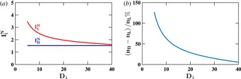
(a) Comparison of the variation of normalized ion current
with Debye number as predicted by the Bohm current formula (2.4) and Laframboise theory
(Narasimhan et al.
Reference Narasimhan and Steinbruchel2001) at
 $((e(V_{s}-V_{pr}))/(k_{B}T_{e}))=20$
. The normalized Bohm and Laframboise current are
represented by
 $I_{B}^{N}$
and
 $I_{L}^{N}$
, respectively. (b) Variation of the
difference in the ion density determined using the Bohm formula (2.4) and the Laframboise theory
with Debye number. The density determined using the Bohm formula and
Laframboise theory are represented by
 $n_{B}$
and
 $n_{L}$
, respectively.

Figure 2(a) shows a
comparison between the normalized ion current collected by the curved surface of a
cylindrical probe as predicted by the Laframboise theory (Narasimhan
et al.
Reference Narasimhan and Steinbruchel2001) and the formula for Bohm current (2.4). The Laframboise current and the
Bohm current are normalized by the factor
 $I^{N}$
, which is given by
 $I^{N}=en_{0}A_{p}\sqrt{k_{B}T_{e}/2\unicode[STIX]{x03C0}m_{i}}$
. Thus for a given density, the ion current predicted by the Bohm
current formula is considerably less at lower Debye numbers. This leads to
over-estimation of the density as shown in figure 2(b). Hence, it is recommended to determine the
density using the Laframboise theory for
 $D_{\unicode[STIX]{x1D706}}\lesssim 35$
.
2.2 Ion current to a Langmuir probe in a collisional plasma
The discussion of the various probe theories so far has been limited to probe
operations at low pressure, where the mean free path of the ions is considerably
greater than the sheath dimensions as well as the probe dimensions. However, as the
operating pressure is increased, the number of neutrals increases, leading to a
decrease in the mean free path of the ions. Ion-neutral collisions in the sheath
surrounding the probe affect the ion current collected by the probe in two major ways
in the OML regime,
 $D_{\unicode[STIX]{x1D706}}\lesssim 3$
.
-
(i) Collisions of positive ions with neutrals in the sheath lead to destruction of their orbital motion. The ions lose their energy and are trapped in the region of high negative potential in the sheath surrounding the probe. These slower ions are unable to escape and ultimately reach the probe. Destruction of ion orbits leads to an increase in the ion current collected by the probe. This effect is dominant when the operating pressure is such that approximately one collision occurs in the sheath (Schulz & Brown Reference Schulz and Brown1955; Zakrzewski & Kopiczynski Reference Zakrzewski and Kopiczynski1974).
-
(ii) Scattering of the positive ions by neutrals leads to a decrease in the ion current collected by the probe. This effect is dominant when the ions collide with a number of neutrals in the sheath (Schulz & Brown Reference Schulz and Brown1955). This reduction in the positive ion current collected by a negatively biased probe due to scattering is dominant at high pressures (Zakrzewski & Kopiczynski Reference Zakrzewski and Kopiczynski1974).
Several attempts have been made to develop a theory to address both these effects of
ion-neutral collisions on the ion current collected by a probe, with varying degrees
of success. One of the earlier rigorous theories to study the effect of collisions on
the current collected by the probe was developed by Chou, Talbot & Willis
(Reference Chou, Talbot and Willis1966) and Talbot & Chou (Reference Talbot and Chou1969). Their theory predicts a reduction in the
probe current due to elastic scattering of charge particles caused by collisions with
neutrals in the sheath and is valid for wide range of Knudsen numbers
 $(0<K_{i}\leqslant \infty )$
. The effect of collisions on the ion current collected by the probe
is calculated as a correction to the normalized collisionless Laframboise ion current
 $(I_{L}^{N})$
.
 $$\begin{eqnarray}I_{i}^{N}=\bar{\unicode[STIX]{x1D6FE}}I_{L}^{N},\end{eqnarray}$$
where
 $I_{i}^{N}$
is the dimensionless ion current collected by the probe, defined as
 $I_{i}^{N}=I_{i}/I^{N}$
, where
 $I_{i}$
is the measured ion current.
The correction coefficient
 $\bar{\unicode[STIX]{x1D6FE}}$
is expressed as
 $$\begin{eqnarray}\frac{1}{\bar{\unicode[STIX]{x1D6FE}}}=1+\frac{J_{i}I_{L}^{N}\unicode[STIX]{x1D70F}^{1/2}}{K_{i}},\end{eqnarray}$$
where
 $J_{i}$
is the integral of the reduced potential over the region between
the undisturbed plasma and the probe. The evaluation of this correction coefficient
is described in appendix C.
The first theory to consider both the increase in probe current due to destruction of
ion orbits and the reduction in ion current due to elastic scattering was proposed by
Zakrzewski & Kopiczynski (Reference Zakrzewski and Kopiczynski1974). They
considered the effects of both of the opposing mechanisms on the ion current
collected by simultaneously multiplying the collisionless Laframboise ion current by
two correction factors,
 $\unicode[STIX]{x1D6FE}_{1}$
and
 $\unicode[STIX]{x1D6FE}_{2}$
, where
 $\unicode[STIX]{x1D6FE}_{1}$
stands for the increase in current due to destruction of orbital
motion and
 $\unicode[STIX]{x1D6FE}_{2}$
, the decrease in current due to scattering. The resulting
normalized dimensionless ion current
 $(I_{i}^{N})$
collected by a cylindrical Langmuir probe in presence of
ion-neutral collisions is given by
 $$\begin{eqnarray}I_{i}^{N}=\unicode[STIX]{x1D6FE}_{1}\unicode[STIX]{x1D6FE}_{2}I_{L}^{N}.\end{eqnarray}$$
In order to account for the increase in ion current due to destruction of the orbital
motions, Zakrzewski & Kopiczynski (Reference Zakrzewski and Kopiczynski1974) argued that in the collisionless limit the current collected by the
probe is given by Laframboise theory
 $(I_{L}^{N})$
, while the ion current at the sheath edge is given by the
Allen–Boyd–Reynolds (ABR) theory
 $(I_{A}^{N})$
(Allen et al.
Reference Allen, Boyd and Reynolds1957; Chen Reference Chen1965b
). Therefore, the current which leaves the sheath due to orbital motion is
given by
 $I_{A}^{N}-I_{L}^{N}$
. In the event of ion-neutral collisions, the number of ions leaving
the sheath due to orbital motion will decrease, thus leading to an increase in probe
current. Zakrzewski & Kopiczynski (Reference Zakrzewski and Kopiczynski1974) proposed a linear increase of the probe current from
 $I_{L}^{N}$
to
 $I_{A}^{N}$
as the number of collisions in the sheath
 $(X_{i})$
increases from
 $0$
to
 $1$
i.e.
 $I_{i}^{N}=I_{L}^{N}+X_{i}(I_{A}^{N}-I_{L}^{N})$
. Therefore,
 $\unicode[STIX]{x1D6FE}_{1}$
may be represented as
 $$\begin{eqnarray}\displaystyle & \displaystyle \unicode[STIX]{x1D6FE}_{1}=1+X_{i}\left(\frac{I_{A}^{N}}{I_{L}^{N}}-1\right)\quad \text{if }X_{i}\leqslant 1, & \displaystyle\end{eqnarray}$$
 $$\begin{eqnarray}\displaystyle & \displaystyle \unicode[STIX]{x1D6FE}_{1}=\frac{I_{A}^{N}}{I_{L}^{N}}\quad \text{if }X_{i}>1. & \displaystyle\end{eqnarray}$$
The reduction in the probe current due to the scattering phenomenon in the sheath is
represented by
 $\unicode[STIX]{x1D6FE}_{2}$
, which is given by
 $$\begin{eqnarray}\displaystyle & \displaystyle \unicode[STIX]{x1D6FE}_{2}=\frac{3-2\,\text{exp}(-X_{i})}{1+2X_{i}}\quad \text{if }X_{i}<1, & \displaystyle\end{eqnarray}$$
 $$\begin{eqnarray}\displaystyle & \displaystyle \unicode[STIX]{x1D6FE}_{2}=\frac{3-\text{exp}(-X_{i})}{2(1+X_{i})}\quad \text{if }X_{i}\geqslant 1. & \displaystyle\end{eqnarray}$$
This reduction factor
 $\unicode[STIX]{x1D6FE}_{2}$
, used by Zakrzewski & Kopiczynski (Reference Zakrzewski and Kopiczynski1974), was proposed by Schulz & Brown (Reference Schulz and Brown1955) and Jakubowski (Reference Jakubowski1972). The number of ion-neutral collisions
 $(X_{i})$
occurring in the sheath can be determined by dividing the sheath
thickness
 $(S_{i})$
by the ion-neutral mean free path
 $\unicode[STIX]{x1D706}_{i}(=1/n_{n}\unicode[STIX]{x1D70E}_{in})$
, where
 $n_{n}$
is the number density of neutrals and
 $\unicode[STIX]{x1D70E}_{in}$
is the ion-neutral collision cross-section. The sheath thickness
around a cylindrical probe can be estimated by using the analytical fit proposed by
Basu & Sen (Reference Basu and Sen1973) based on the numerical
calculations carried out by them.
 $$\begin{eqnarray}\displaystyle S_{i}=\unicode[STIX]{x1D706}_{D}\sqrt{m(|\unicode[STIX]{x1D702}|+3.5)-4}\quad \text{if }|\unicode[STIX]{x1D702}|\geqslant 3\text{ and }0.1\leqslant D_{\unicode[STIX]{x1D706}}\leqslant 10, & & \displaystyle\end{eqnarray}$$
where
 $m\simeq 0.59+1.86D_{\unicode[STIX]{x1D706}}^{0.47}$
and
 $\unicode[STIX]{x1D702}=e(V_{s}-V_{pr})/k_{B}T_{e}$
.
The theory of Zakrzewski & Kopiczynski (Reference Zakrzewski and Kopiczynski1974) is valid up to a few collisions within the probe sheath in the OML
regime. Rousseau, Teboul & Bchu (Reference Rousseau, Teboul and Bchu2005)
compared the density determined from the positive ion probe current using the theory
of Zakrzewski & Kopiczynski (Reference Zakrzewski and Kopiczynski1974) with
microwave autointerferometry measurements and observed excellent agreement. They
varied the number of collisions in the probe sheath from less than
 $1$
to
 $7$
in their experimental study. In terms of Debye number and Knudsen
number, the region of validity (Tichý et al.
Reference Tichý, S̃ícha, David and David1994) may be written as
 $D_{\unicode[STIX]{x1D706}}\lesssim 3$
and
 $0.5\lesssim K_{i}<\infty$
.
The limitation in the applicability of the theory of Zakrzewski & Kopiczynski
(Reference Zakrzewski and Kopiczynski1974) to lower Knudsen numbers in the OML
regime is because of the usage of the correction factor
 $\unicode[STIX]{x1D6FE}_{2}$
(2.11) which has
been derived by Jakubowski (Reference Jakubowski1972) under the
assumption of few collisions in the probe sheath. Tichý
et al. (Reference Tichý, S̃ícha, David and David1994)
extended the regime of validity to arbitrary Knudsen number
 $(K_{i})$
by determining the correction due to elastic scattering of ions in
the probe sheath using the theory of Talbot & Chou (Reference Talbot and Chou1969).
 $$\begin{eqnarray}I_{i}^{N}=\unicode[STIX]{x1D6FE}_{1}\bar{\unicode[STIX]{x1D6FE}_{2}}I_{L}^{N},\end{eqnarray}$$
where
 $\bar{\unicode[STIX]{x1D6FE}_{2}}=\bar{\unicode[STIX]{x1D6FE}}$
, refer to (2.6).
This model proposed by Tichý et al. (Reference Tichý, S̃ícha, David and David1994) is called the ‘modified Talbot and
Chou model’. It is valid for any Knudsen number
 $(0\lesssim K_{i}<\infty )$
within the OML regime
 $D_{\unicode[STIX]{x1D706}}\lesssim 3$
. The prediction of this model was found to be in agreement with
simulation results by Iza & Lee (Reference Iza and Lee2006).
Ion density determined from ion current in the presence of collisions using the
modified Talbot and Chou model was found to be in agreement with the electron density
measured from the electron current by Chudáček
et al. (Reference Chudáček, Kudrna, Glosik, Šícha and Tichỳ1995) in a
flow after a glow plasma. Chudáček et al.
(Reference Chudáček, Kudrna, Glosik, Šícha and Tichỳ1995) carried out the experimental study
at densities and neutral pressures ranging from
 $10^{6}$
to
 $10^{10}~\text{cm}^{-3}$
and 60 Pa to 150 Pa, respectively.
The theories discussed thus far in this section are being used to determine the plasma density from the positive ion probe current over a wide operating range which is relevant to most laboratory dusty plasma experiments, from the collisionless to the collisional regime at intermediate pressure, and for a wide range of Debye numbers. The theories have been tested by different authors as mentioned above over a wide operating range by employing various methods having varying degrees of complexities. Although, the theories take into account the various confounding issues associated with interpretation of Langmuir probe current voltage characteristics, ultimately it will be necessary to compare probe measurements with some other diagnostic that is less complicated to interpret over the complete range of validity of the probe theories.
3 Bohm criterion for a dusty plasma sheath
The ion density is determined from the ion current collected by the probe in the thin
sheath regime using the Bohm current formula. According to the Bohm criterion (Bohm
Reference Bohm1949), in the absence of dust in the plasma the
ions enter the sheath with a velocity either equal to or greater than the Bohm velocity.
Mathematically, it may be written as
 $M\geqslant 1$
, where
 $M=v_{i0}/v_{B}$
,
 $v_{i0}$
is the velocity of the ions at the sheath edge and
 $v_{B}$
is the Bohm velocity (ion sound speed). The Bohm sheath criterion was
experimentally verified by Lee et al. (Reference Lee, Severn, Oksuz and Hershkowitz2006) by measuring the velocity of argon ions using laser induced
fluorescence (LIF). Their LIF findings showed that the argon ions approached the Bohm
velocity near the sheath boundary in the pure argon plasma. The presence of dust in a
dusty plasma sheath modifies the Bohm criterion. The Bohm criterion in a dusty plasma
has been theoretically studied by many authors (Yu, Saleem & Luo Reference Yu, Saleem and Luo1992; Ma & Yu Reference Ma and Yu1995; Liu et al.
Reference Liu, Wang, Wang, Zhang, Zou and Zhang2003; Yaroshenko et al.
Reference Yaroshenko, Verheest, Thomas and Morfill2009; Chung Reference Chung2014; Fouial, Tahraoui & Annou Reference Fouial, Tahraoui and Annou2016) under a variety of scenarios; however, an experimental
cross-verification of various theoretical results remains to be carried out. In a dusty
plasma, the ions approach the sheath typically with a velocity greater than the ion
sound speed. For a dusty plasma sheath consisting of electrons following the Boltzmann
distribution, cold ions and immobile dust grains in the absence of dust charge
fluctuations, the Bohm criterion is given by
 $M>M_{c}$
(Shukla & Mamun Reference Shukla and Mamun2001),
where
 $M_{c}$
is the critical Mach number.
 $M_{c}$
is given by the formula,
 $M_{c}=\sqrt{\unicode[STIX]{x1D6FF}}$
, where
 $\unicode[STIX]{x1D6FF}=n_{i0}/n_{e0}$
,
 $n_{i0}$
and
 $n_{e0}$
are equilibrium density of ions and electrons, respectively. However,
when the effect of dust charge fluctuation is included, the Bohm criterion (Ma &
Yu Reference Ma and Yu1995) continues to be
 $M>M_{c}$
but
 $M_{c}$
in this case is given by,
 $$\begin{eqnarray}M_{c}=\frac{-\unicode[STIX]{x1D6FF}+2Q_{d0}+\sqrt{(3\unicode[STIX]{x1D6FF}-2Q_{d0})^{2}+8(\unicode[STIX]{x1D6FF}-1)\left\{2-(3\unicode[STIX]{x1D6FF}-2)/Q_{d0}\right\}}}{2\left\{1-(\unicode[STIX]{x1D6FF}-1)/Q_{d0}\right\}},\end{eqnarray}$$
where
 $Q_{d0}$
is the normalized dust charge at the sheath edge.
A closer look at both of the formulas for ion velocity at the sheath edge in a dusty
plasma suggests that the modification in ion velocity in dusty plasmas for a number of
experiments may be negligibly small. For example, considering the following experimental
parameters, the ion density,
 $n_{i0}\sim 10^{9}~\text{cm}^{-3}$
, dust density,
 $n_{d0}\sim 10^{4}~\text{cm}^{-3}$
and dust charge,
 $q_{d0}\sim 5\times 10^{3}\text{e}^{-1}$
, and the quasineutrality condition,
 $n_{i0}=n_{e0}+n_{d0}q_{d0}$
, one obtains
 $n_{e0}=0.95n_{i0}$
. Therefore
 $\unicode[STIX]{x1D6FF}$
turns out to be 1.05 and the corresponding calculated value of
 $M_{c}(=\sqrt{\unicode[STIX]{x1D6FF}})$
is 1.02.
4 Design of Langmuir probe systems for measurement in a complex plasma experimental device
The design of a Langmuir probe diagnostic system developed for measuring density and
electron temperature in a dusty plasma in the complex plasma experimental device (CPED)
is described in this section. A detailed description of CPED is given by Kaur
et al. (Reference Kaur, Bose, Chattopadhyay, Sharma, Ghosh and Saxena2015a
, Reference Kaur, Bose, Chattopadhyay, Ghosh and Saxena2016). Argon plasma is produced by
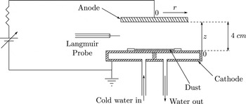
applying a potential difference between coaxially arranged disc electrodes. The cathode
surface is partially covered with mono-dispersed melamine formaldehyde (MF) dust
particles of diameter
 $6.48~\unicode[STIX]{x03BC}\text{m}$
and mass density
 $1.51~\text{g}~\text{cm}^{-3}$
, as shown in figure 3. The
cathode is cooled actively by cold water to prevent the heating of neutrals near the
cathode surface. The anode to cathode voltage is varied from 230 to 270 V during
the experiments. The neutral pressure is varied from 50 to 300 Pa during
different experiments in CPED. The cylindrical Langmuir probe used for acquiring the
 $I$
–
 $V$
characteristics is inserted radially.
4.1 Langmuir probe design
An ultra-thin cylindrical single Langmuir probe is used for determining local plasma
parameters in dusty plasma experiments such that the disturbance caused by it on the
ambient dust structures is minimal. The minimum dimension of the Langmuir probe is
dictated by the requirement to acquire enough current such that a high signal to
noise ratio can be maintained. Also the probe dimension must be such that a well
defined Langmuir probe theory exist for interpretation of the
 $I$
–
 $V$
characteristics.
A tungsten wire of
 $62.5~\unicode[STIX]{x03BC}\text{m}$
radius
 $(r_{p})$
and 6 mm length
 $(l_{p})$
is used to make the cylindrical Langmuir probe to ensure minimum
perturbation. The length and radius of the probe are carefully chosen to ensure that
 $l_{p}/r_{p}\gg 1$
, such that cylindrical probe theory can be used for analysing the
probe data. The Langmuir probe measurements are to be carried out over a wide range
of neutral pressure varying from 50 to 350 Pa. The mean free path of the ions
due to ion-neutral collisions is expected to vary from 40 to 5.7
 $\unicode[STIX]{x03BC}\text{m}$
and the corresponding Knudsen number varies from
 $0.64$
to
 $0.09$
. The mean free path of the ions in the presence of ion-neutral
collisions is determined by using the formula
 $\unicode[STIX]{x1D706}_{in}=1/(n_{n}\unicode[STIX]{x1D70E}_{in})$
, where
 $n_{n}=P/k_{B}T_{n}$
. The argon ion-neutral momentum transfer collision cross-section is
estimated using the analytical approximation given by Phelps (Reference Phelps1994). The ion density is expected to vary in the range
 $5\times 10^{8}$
–
 $5\times 10^{9}~\text{cm}^{-3}$
while the electron temperature is expected to be approximately
 $1$
eV, therefore the Debye number is expected to vary in the
range
 $0.2$
–
 $0.57$
. The expected ranges of Debye number and Knudsen number lie within
the region of validity of the modified Talbot–Chou model (Tichý
et al.
Reference Tichý, S̃ícha, David and David1994), which is valid for any Knudsen number
 $(0\lesssim K_{i}<\infty )$
within the OML regime
 $D_{\unicode[STIX]{x1D706}}\lesssim 3$
. Thus, the requirement of a well-defined theory for interpreting
the probe characteristics is satisfied.
Schematic of the experimental set-up.

4.2 Probe instrumentation
Designing of Langmuir probe circuits for acquiring the
 $I$
–
 $V$
characteristics in a dusty plasma using an ultra-thin Langmuir
probe requires effective resolution of several issues. The magnitude of the ion
current collected by an ultra-thin probe at low density plasma is a few
 $\unicode[STIX]{x03BC}A$
or less. Hence, special attention is to be paid to the shielding
and grounding of the Langmuir probe circuit (Brookshier Reference Brookshier1969; Ott Reference Ott1976; Rich Reference Rich1983).
Generalized circuit description of commonly used Langmuir probe circuit with a floating current measuring resistance.

In order to minimize the contamination of the Langmuir probe by charged dust
particles the
 $I$
–
 $V$
characteristics are to be acquired by sweeping the bias voltage of
the probe at high frequency, approximately 100 Hz (refer to
§ 4.3). At this frequency,
the commonly used Langmuir probe circuit layout consisting of a coaxial cable with a
grounded shield, connecting the probe tip to the sweep generator, can no longer be
used. At 100 Hz the coaxial cable may be thought of as a cylindrical capacitor
as shown in figure 4. Rapid variation of
potential in the central conductor of the coaxial cable with respect to the grounded
outer shield results in a displacement current given by
 $I_{cap}\approx C_{c}\times \text{d}V_{in}/\text{d}t$
, where
 $C_{c}$
is the cable capacitance. Therefore, the current in the Langmuir
probe circuit is the summation of the capacitive current
 $(I_{cap})$
and the probe current due to the collection of charged particles
 $(I_{p})$
. A commonly used coaxial cable for wiring a Langmuir probe circuit
is RG 58, which has a capacitance of
 ${\sim}100~\text{pF m}^{-1}$
between the inner conductor and the outer shield. Generally,
Langmuir probe cable used for laboratory experiments can be a few metres long. If one
considers the application of
 $100$
V peak to peak triangular waveform to bias a Langmuir probe
connected to a 2 m long cable, the displacement current between the central
conductor and outer shield turns out to be
 $4~\unicode[STIX]{x03BC}A\{I_{cap}=(200\times 10^{-12}~\text{F})\times (100~\text{V}/200^{-1}~\text{s})\}$
, which is comparable to the current collected by a negatively
biased probe in the pure ion current region in a low density plasma
 $(10^{8}-10^{9}~\text{cm}^{3})$
. If the contribution from the capacitive current is not removed
from the total current
 $(I_{R}=I_{p}+I_{cap})$
to determine the probe current due to the collection of electrons
and ions then the determination of the plasma parameters from the
 $I$
–
 $V$
characteristics will be highly erroneous. The Langmuir probe
circuit of CPED is specifically designed to acquire
 $I$
–
 $V$
characteristics with high signal to noise ratio by minimizing the
sources of unwanted signals.
4.2.1 Langmuir probe circuit of CPED
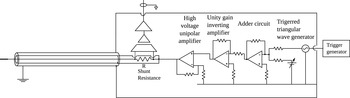
Schematic of the Langmuir probe circuit used for acquiring
 $I$
–
 $V$
characteristics in CPED.

The Langmuir probe circuit designed for acquiring
 $I$
–
 $V$
characteristics in CPED is shown in figure 5. It consist of a Langmuir probe connected in
series with a floating shunt resistance (current measuring resistance) and a
grounded triangular wave generator used to sweep the probe bias. The probe tip is
connected to the current measuring resistance using a triaxial cable. The triaxial
cable, as shown in figure 5, typically
comprises a central conductor and two coaxially placed outer shields isolated from
each other. The central conductor of the triaxial cable connects the probe tip to
the current measuring resistance. The current measuring resistance is housed in an
aluminium box and the body of the box is connected to the triangular wave
generator at one end, while at the other end it is connected to the inner shield
of the triaxial cable, as shown in figure 5. The central conductor is driven by the triangular wave generator
through the current measuring resistance, while the inner shield is driven by the
triangular wave generator through the aluminium box housing the current measuring
resistance. By driving the central conductor and the inner shield (guard) using
the same voltage source, one can in effect remove the potential difference between
the central conductor and the driven guard. In the absence of driving potential
difference between the central conductor and the inner shield, the capacitive
current between the two conductors is minimized. The outer shield of the triaxial
cable is suitably grounded (Ott Reference Ott1976) to
reduce pick up of spurious voltages due to coupling with various noise sources in
the laboratory and the central conductor.
In CPED, plasma is produced by parallel plate direct current (DC) discharge with a
grounded cathode; the potential in the positive column with respect to the
grounded cathode may be as high as
 ${\sim}250$
V. Therefore, a high voltage triangular wave generator is
designed for acquiring the
 $I$
–
 $V$
characteristics. At the heart of the triangular wave generator
is an APEX high voltage
 $(+440~\text{V})$
operational amplifier (PA 85), which is operated in
unipolar mode. The input to the power amplifier is fed by an adder circuit. It
superimposes a triangular waveform on a constant DC voltage to produce a
triangular waveform with a positive offset. This triangular waveform with a
positive offset is amplified by a high voltage operational amplifier (PA 85) to
produce the probe bias voltage.
4.2.2 Demonstration of the removal of capacitive pick up
The effectiveness of a triaxial cable with a driven guard in reducing capacitive
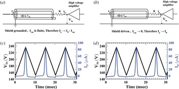
current in a Langmuir probe circuit is shown in figure 6. Langmuir probe
 $I$
–
 $V$
characteristics are acquired in two different configurations of
the probe circuit. In the first case, the inner shield of the triaxial cable is
connected to the outer grounded shield as shown in figure 6(a). In this case, the probe
circuit reduces to a commonly used circuit with a coaxial cable connecting the
probe tip to the floating current measuring resistance. In the second case, the
inner shield of the triaxial cable is driven by the triangular wave generator as
shown in figure 6(b).
 $I$
–
 $V$
characteristics are acquired in a DC glow discharge plasma by
sweeping the Langmuir probe at 100 Hz in both circuit configurations.
(a) Schematic of the Langmuir probe circuit using
triaxial cable, (a) with the inner shield connected to
the outer grounded shield and (b) with the driven inner
shield. Langmuir probe
 $I$
–
 $V$
characteristics acquired using 100 Hz sweep in
the presence of a plasma, (c) when inner shield is
grounded and (d) inner shield is driven. The
 $I$
–
 $V$
characteristics become distorted due to the capacitive
current between the central conductor and grounded shield, when the inner
shield is grounded. The probe is located at
 $r=6.5$
cm and
 $z=9$
mm and discharge parameters are
 $I_{Dis}=27$
mA and pressure 160 Pa.

The
 $I$
–
 $V$
characteristics acquired using the circuit shown in
figure 6(a)
clearly exhibit distortions due to the capacitive current between the central
conductor and the inner grounded shield, as observed in figure 6(c). The rising part of the
triangular bias voltage is observed to increase the probe current, while the
falling part decreases the probe current. This is so because the capacitive
current between the central conductor and the grounded shield is positive when the
bias voltage rises with time while it is negative when the probe bias decreases
with time,
 $I_{cap}\propto \text{d}(V_{in}-V_{R})/\text{d}t$
. In order to further confirm the role of the capacitive current
 $(I_{cap})$
in the distortion of the
 $I$
–
 $V$
characteristics, the
 $I_{cap}$
between the central conductor and the grounded shield is
calculated and compared with distortion in the
 $I$
–
 $V$
characteristics observed in figure 6(c). First, the capacitance between the
central conductor and the inner grounded shield is determined by using the
relation
 $I_{cap}\approx C(V_{in}/\text{d}t)$
and measuring the probe current while sweeping the probe bias in
the absence of a plasma. The measured capacitance is found to be 91 pF. In
figure 6(c) the
 $I$
–
 $V$
characteristics are acquired by using a triangular waveform to
sweep the probe bias from 152 to 236.4 V. Therefore, the calculated peak to
peak capacitive current is,
 $I_{cap_{pp}}=3.1~\unicode[STIX]{x03BC}A$
. The difference in the ion current of the
 $I$
–
 $V$
characteristics (refer figure 6
c) for the increasing and decreasing probe bias is
 $3~\unicode[STIX]{x03BC}A$
. This agreement between the calculated magnitude of the
capacitive current and the difference in the ion current for the increasing and
decreasing probe bias clearly confirms that the distortion in the
 $I$
–
 $V$
characteristics is due to the capacitive current.
In the second case, when the inner shield of the triaxial cable is driven by the
triangular wave generator, the acquired
 $I$
–
 $V$
characteristics, shown in figure 6(d), do not exhibit any distortion due to the
capacitive current. Hence, the voltage drop across the current measuring
resistance is dominated by the collection of electrons and ions by the Langmuir
probe. In order to further ensure that there is no significant effect of the
capacitive current on the measured probe current, the
 $I$
–
 $V$
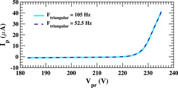
characteristics are acquired by sweeping the probe bias at two
frequencies, 52.5 Hz and 105 Hz, respectively. Since the capacitive
current is dependent on the frequency of the probe bias, a change in the probe
bias frequency (frequency of the triangular waveform) will alter the capacitive
current. Thus, if the capacitive current contributes significantly to the
potential drop across the current measuring resistance
 $R$
(refer to figure 6
b) then the measured probe current at two bias frequencies will
be different. The
 $I$
–
 $V$
curves acquired at 52.5 Hz and 105 Hz probe bias
frequency were superposed and both the
 $I$
–
 $V$
curves were found to be in very good agreement, as shown in
figure 7. This confirms the
effective removal of the capacitive current, as the acquired
 $I$
–
 $V$
characteristics are independent of the frequency of the probe
bias sweep.
Superposition of
 $I$
–
 $V$
characteristics acquired using a triangular waveform of
frequency 52.5 Hz and 105 Hz. Probe is located at
 $r=6.5$
cm and
 $z=9$
mm. Discharge parameters are
 $I_{Dis}=27$
mA and pressure
 $170$
Pa. Langmuir probe circuit with driven inner
shield as shown in figure 6(b) is used for acquiring
 $I$
–
 $V$
characteristics.

4.3 Minimization of dust contamination
Most dusty plasma experiments, in the laboratory, are carried out using dielectric
dust particles. Dust particles can acquire large charges (Goree Reference Goree1994) depending on their size, ambient plasma conditions, etc.
Generally, dust particles become negatively charged because of the higher mobility of
the electrons compared to that of the ions. These negatively charged dust particles
deposit on the probe surface, reducing the current collecting area of the probe. This
leads to error in the interpretation of the
 $I$
–
 $V$
characteristics.
Comparison of
 $I$
–
 $V$
characteristics of a clean and dust contaminated Langmuir
probe acquired in a DC glow discharge dusty plasma in CPED. Probe is located at
 $r=5$
cm and
 $z=1.5$
cm. Discharge parameters are
 $I_{Dis}=25$
mA and pressure 150 Pa.

Figure 8 shows a comparison of
 $I$
–
 $V$
curves acquired by a clean and a dust contaminated probe. Both the
 $I$
–
 $V$
curves are acquired in a DC glow discharge dusty plasma at
 $150$
Pa neutral pressure and a
 $25$
mA discharge current. The measurement is carried out at
 $r=4$
cm and
 $z=1.5$
cm. The floating potential determined from the
 $I$
–
 $V$
curves of both the contaminated and the clean probe are found to be
 $200$
V, however the current collected by the contaminated probe
is less than the current collected by the clean probe.
A multitude of methods (Hayashi Reference Hayashi2001; Kim
& Merlino Reference Kim and Merlino2006; Klindworth
et al.
Reference Klindworth, Arp and Piel2007; Bilik et al.
Reference Bilik, Anthony, Merritt, Aydil and Kortshagen2015) have been devised in the past to minimize
probe contamination with varying degrees of success and complexity. We have minimized
the dust contamination by utilizing the slow response time and negative charge of the
dust particles in a dusty plasma. The Langmuir probe, on insertion into a dusty
plasma, is held at a potential much less than the floating potential, as shown in
figure 9, such that the electric field
between the Langmuir probe and the plasma repels the negatively charge dust
particles. The
 $I$
–
 $V$
characteristics are acquired by sweeping the probe bias potential
using a fast triangular waveform such that the fundamental frequency of the waveform
is much greater than the dust plasma frequency, as shown in figure 9. Since the frequency of the applied triangular
waveform to bias the probe is much higher than the dust plasma frequency, the dust
particles are not expected to be modulated by the probe bias. Hence, the dust
particles are no longer attracted by the positively biased probe. Thus minimizing
contamination of the probe surface by dust particles.
(a) Constant voltage applied to the Langmuir probe to bias
it in the ion current region. (b) A triangular waveform
superimposed on the constant DC voltage to acquire the
 $I{-}V$
characteristics.

A dust plasma frequency of
 $10$
Hz is considered for determining the frequency of the probe
sweep for acquiring the
 $I$
–
 $V$
characteristics. It is calculated using the well-known formula
 $f_{pd}=1/2\unicode[STIX]{x03C0}(n_{d0}q_{d0}^{2}\text{e}^{2}/\unicode[STIX]{x1D716}_{0}m_{d})^{1/2}$
, where
 $f_{pd}$
is the dust plasma frequency,
 $n_{d0}$
is the dust density,
 $q_{d0}$
is the dust charge,
 $m_{d}$
is the mass of the dust particle,
 $\unicode[STIX]{x1D716}_{0}$
is the permittivity of free space and
 $e$
is the electronic charge. The negative charge acquired by a dust
particle in a plasma is estimated by considering the dust particle to be a condenser
of capacitance
 $C_{d}$
and the charge acquired by the dust particle is given by
 $Q_{d}=q_{d0}\,e=C_{d}\unicode[STIX]{x1D6F7}_{d}$
. Thus, the dust charge can be calculated by determining the
capacitance and potential of the dust particle. The capacitance of the dust particle
(Melzer Reference Melzer2016) is given by
 $C_{d}=4\unicode[STIX]{x03C0}\unicode[STIX]{x1D716}_{0}r_{d}(1+r_{d}/\unicode[STIX]{x1D706}_{DS})$
, where
 $r_{d}$
is the radius of the dust particle and
 $\unicode[STIX]{x1D706}_{DS}$
is the linearized Debye length. For plasma with subthermal ion flow
and
 $T_{e}\gg T_{i}$
as in CPED,
 $\unicode[STIX]{x1D706}_{DS}$
is approximately given by the ion Debye length,
 $\sqrt{\unicode[STIX]{x1D716}_{0}k_{B}T_{i}/n_{0}\text{e}^{2}}$
. The potential of the dust particle,
 $\unicode[STIX]{x1D6F7}_{d}$
, in gas discharge plasmas can be written as
 $\unicode[STIX]{x1D6F7}_{d}\sim -\unicode[STIX]{x1D6FC}T_{e}/e$
. The numerical coefficient
 $\unicode[STIX]{x1D6FC}$
is determined by the balance of the ion and electron current fluxes
on the surface of the dust particle. For experiments at high neutral pressure
 ${\sim}100$
Pa, the ion flux,
 $\unicode[STIX]{x1D6E4}_{ion}$
incident on the surface of the dust particle is affected by
ion-neutral collisions. The ion flux in the presence of ion-neutral collisions is
calculated using the interpolation formula derived by Khrapak & Morfill (Reference Khrapak and Morfill2008). The electron-neutral mean free path is
typically two orders of magnitude greater than the ion-neutral mean free path. Hence,
the electrons are collisionless. The collisionless electron flux to the dust particle
is given by the OML theory,
 $\unicode[STIX]{x1D6E4}_{e}=\sqrt{8\unicode[STIX]{x03C0}}r_{d}^{2}n_{0}v_{Te}\exp (-\unicode[STIX]{x1D6FC})$
.
In CPED, the ion density is typically approximately
 ${\sim}10^{9}~\text{cm}^{-3}$
, the electron temperature is approximately
 ${\sim}1.5$
eV. Dust densities as high as
 $10^{4}$
cm
 $^{-3}$
have been observed by Kaur et al. (Reference Kaur, Bose, Chattopadhyay, Sharma, Ghosh, Saxena and Thomas2015b
) in CPED. At 100 Pa neutral pressure, the ion mean free path of argon
ions is estimated to be
 $20~\unicode[STIX]{x03BC}\text{m}$
. Using the above mentioned parameters, the dust charge is
calculated to be 4880 e. The dusty plasma experiments are carried out using
spherical melamine formaldehyde dust particle of radius
 $3.24~\unicode[STIX]{x03BC}\text{m}$
and mass
 $2.15\times 10^{-13}$
kg. The dust plasma frequency calculated by plugging the
dust mass, dust charge and
 $10^{4}~\text{cm}^{-3}$
dust density in the formula for dust plasma frequency turns out to
be
 ${\sim}9$
Hz.
The
 $I$
–
 $V$
characteristics are acquired by applying a single triangular
waveform of frequency
 ${\sim}100$
Hz to bias the probe. While acquiring
 $I$
–
 $V$
characteristics in a DC glow discharge dusty plasma, the ion
current collected by the probe at the constant negative potential, at which the probe
is held in between two triangular sweeps, is monitored. The probe is cleaned when the
ion current collected by the probe decreases to less than
 $90\,\%$
of the maximum value under similar discharge conditions at the same
location. The cleaning procedure involves biasing it in the high electron current
region as described by Klindworth et al. (Reference Klindworth, Arp and Piel2007) before reuse. We are able to obtain several
 $I$
–
 $V$
traces by following the above mentioned procedure, before cleaning
is required. Figure 10 shows the
decrease in probe current as a function of number of sweeps. The measurements are
carried out at
 $165$
Pa argon neutral pressure and 27 mA discharge
current. The probe is located at
 $r=6.2$
cm and
 $z=8$
mm in the middle of a rotating dense dust structure.
Probe current at
 $V_{pr}=204$
V with respect to the initial value of current
collected by a clean probe over a number of voltage sweeps in a dense
rotating dust structure. The measurements are carried out at
 $I_{Dis}=27$
mA, argon neutral pressure
 $165$
Pa,
 $r=6.2$
cm and
 $z=8$
mm.

Following the establishment of the method of acquiring
 $I$
–
 $V$
characteristics in a dusty plasma, probe characteristics acquired
in the presence and absence of dust in the plasma are compared. A
 $5\,\%$
reduction in the electron current is observed in the presence of
dust in the plasma. The reduction percentage is calculated by measuring and comparing
the electron current acquired at the plasma potential. Both the measurements are
carried out at the same location and for the same discharge parameters. The argon
neutral pressure is maintained at 155 Pa and the discharge current is held at
26 mA. Probe is located at
 $r=6.5$
cm and
 $z=8$
mm. The reduction in electron current of the Langmuir probe
in the presence of dust particles is consistent with observations of other
researchers (Trottenberg et al.
Reference Trottenberg, Brede, Block and Piel2003; Adhikary et al.
Reference Adhikary, Bailung, Pal, Chutia and Nakamura2007; Klindworth et al.
Reference Klindworth, Arp and Piel2007; Goertz, Greiner & Piel Reference Goertz, Greiner and Piel2011) in a laboratory dusty plasma. The loss of
electrons from the plasma to charge dust particles may contribute to the reduction in
the electron current collected by the probe.
5 Principles of the evaluation procedure of Langmuir probe
 $I$
–
$V$
characteristics


Figure 11(a) shows a
typical Langmuir probe
 $I$
–
 $V$
characteristic obtained in CPED. For determining the plasma parameters
from the Langmuir probe data, they are first smoothed using the Savitzky–Golay
method (Savitzky & Golay Reference Savitzky and Golay1964; Magnus
& Gudmundsson Reference Magnus and Gudmundsson2008), if necessary. This is
followed by determination of the plasma potential. A brief discussion on the smoothing
of the probe
 $I$
–
 $V$
characteristics is presented in appendix A.
5.1 Determination of plasma potential
The space potential or the plasma potential may be easily determined from the
 $I$
–
 $V$
characteristics using the tangent or the derivative method. In the
tangent method, the space potential is estimated from the point of intersection of
tangents drawn in the electron retarding and electron saturation region in the
semi-logarithmic curve of probe current versus probe potential, as shown in
figure 11.
(a)
 $I$
–
 $V$
characteristics acquired using the Langmuir probe.
(b) Variation of the first derivative of the probe
current with the probe potential. (c) Variation of
 $\ln I_{P}$
with the probe potential. (d) Variation
of the second derivative of the probe current with the probe potential.
Discharge parameters are
 $I_{Dis}=30$
mA and pressure is 66 Pa and the probe is
located at
 $3.5$
cm.

In the method of derivatives, the space potential is derived from the
 $I$
–
 $V$
characteristics by making use of the fact that the maximum of the
first derivative of the probe current
 $(I_{p}^{^{\prime }})$
and the zero crossing point of the second derivative of the probe
current
 $(I_{p}^{\prime \prime })$
correspond to the space potential. The determination of the space
potential using the method of derivatives is preferred as it is more sensitive to
changes in the probe current, especially the method of second derivative (Kagan
et al.
Reference Kagan and Perel1964). Collisions of the charged particles in
the sheath surrounding the probe may lead to rounding of the probe characteristics as
a result of which the inflection point may not correspond to the plasma potential.
The influence of collisions on the determination of the plasma potential from the
second derivative method may be neglected if the following condition is satisfied
(Klagge & Tichỳ Reference Klagge and Tichỳ1985).
 $$\begin{eqnarray}\frac{K_{e}(K_{e}+1)}{K_{e}+\ln \left({\displaystyle \frac{l_{p}}{r_{p}}}\right)}>1.\end{eqnarray}$$
The
 $I$
–
 $V$
curve shown in figure 11(a) is acquired at 66 Pa using a single Langmuir
probe of diameter 0.125 mm and length 6 mm. For our experimental
conditions
 $((K_{e}(K_{e}+1))/(K_{e}+\ln (l_{p}/r_{p})))$
for a
 $0.6$
eV electron is 159, which is much greater than 1.
Hence, the plasma potential may be determined using the derivative method. The
determination of the space potential using the derivative method is illustrated in
figure 11(b,d).
The derivative of the probe current, shown in figure 11(b), is estimated by sliding a second-order
polynomial of the form
 $I_{p}=aV_{pr}^{2}+bV_{pr}+c$
in the
 $I$
–
 $V$
trace covering an odd number of points
 $(m)$
in each fit. The differentiated value
 $\text{d}I_{p}/\text{d}V_{pr}$
at the
 $(m+1)/2$
th data point is determined by
 $\text{d}I_{p}/\text{d}V_{pr}|_{m+1/2}=2aV_{pr}|_{m+1/2}+bV_{pr}|_{m+1/2}$
. We suggest the determination of the plasma potential from the zero
crossing of the second derivative of the probe current for automatic determination of
the plasma potential from the
 $I$
–
 $V$
characteristics using a computer program.
5.2 Determination of electron temperature
The electron temperature is determined from the electron current collected by the
Langmuir probe in the electron retarding region of the
 $I$
–
 $V$
characteristics. In a plasma where electrons are in thermal
equilibrium, the electron current collected by a probe for probe potential
 $(V_{pr})$
less than the plasma potential (space potential) is given by (Chen
Reference Chen1965a
),
 $$\begin{eqnarray}I_{e}=I_{e0}\exp \left\{\frac{e(V_{pr}-V_{s})}{k_{B}T_{e}}\right\}\quad V_{pr}\leqslant V_{s},\end{eqnarray}$$
where
 $I_{e0}=A_{p}n_{0}(k_{B}T_{e}/2\unicode[STIX]{x03C0}m_{e})^{1/2}$
,
 $V_{pr}$
is the probe potential with respect to the reference electrode and
 $V_{s}$
is the plasma (space) potential. Thus, it is observed from (5.2) that
 $\ln I_{e}$
varies linearly with the probe potential
 $(V_{pr})$
in the electron retarding region
 $(V_{pr}\leqslant V_{s})$
and the inverse of the slope of this straight line gives the
electron temperature. Often, in plasma discharges instead of a single Maxwellian
distribution of electrons with temperature
 $T_{e}$
, there are two distinct distributions. One Maxwellian distribution
corresponds to cold (bulk) electrons having temperature
 $T_{ec}$
while the other represents the hot electrons
 $(T_{eh})$
, where
 $T_{eh}>T_{ec}$
. The electron current collected by a probe in the electron
retarding region in a bi-Maxwellian plasma is given by (Godyak, Meytlis &
Strauss Reference Godyak, Meytlis and Strauss1995; Choi, Chung & Youn Moon
Reference Choi, Chung and Youn Moon2013)
 $$\begin{eqnarray}I_{e}=I_{ec0}\exp \left\{\frac{e(V_{pr}-V_{s})}{k_{B}T_{ec}}\right\}+I_{eh0}\exp \left\{\frac{e(V_{pr}-V_{s})}{k_{B}T_{eh}}\right\}\quad V_{pr}\leqslant V_{s},\end{eqnarray}$$
where
 $I_{ec0}=A_{p}n_{ec}(k_{B}T_{ec}/2\unicode[STIX]{x03C0}m_{e})^{1/2}$
and
 $I_{eh0}=A_{p}n_{eh}(k_{B}T_{eh}/2\unicode[STIX]{x03C0}m_{e})^{1/2}$
,
 $n_{ec}$
and
 $n_{eh}$
represent the density of cold (bulk) and hot electrons,
respectively. The total electron density is represented by
 $n_{0}\approx n_{e}=n_{ec}+n_{eh}$
. The curve of
 $\ln I_{e}$
versus probe potential in this case has two linear regions, one
corresponding to hot electrons and the other representing cold electrons, as shown in
figure 12.
(a)
 $I$
–
 $V$
characteristics of the Langmuir probe and the fitted ion
current. (b) Variation of
 $\ln I_{e}$
with probe potential.

However, the current collected by a probe in the electron retarding region consists
of both the electron and ion current. The ion current can be removed from the probe
current by making use of the linear dependence of the square of the ion current on
probe potential (Chen Reference Chen1965c
, Reference Chen2001), for Langmuir probe
measurements in the collisionless regime using a thin probe. The ion current part of
the
 $I$
–
 $V$
characteristics at sufficiently negative probe potential is fitted
with
 $I_{i}=K_{c}(V_{s}-V_{pr})^{1/2}$
(Neumann, Kammeyer & Schneemann Reference Neumann, Kammeyer and Schneemann1995) and extrapolated to
 $I_{i}=0$
, where ‘
 $K_{c}$
’ is a constant. The fitted curve is then subtracted from the
total probe current to obtain the electron current.
In the presence of ion-neutral collisions in the sheath surrounding the probe, the square of the ion current collected by the probe is no longer linearly dependent on the probe potential (Trunec, Španěl & Smith Reference Trunec, Španěl and Smith1995). The ion current can be removed from the probe current by using the below mentioned empirical formula (Nuhn & Peter Reference Nuhn and Peter1977; David et al. Reference David, S̃ícha, Tichý, Kopiczynski and Zakrzewski1990)
 $$\begin{eqnarray}I_{i}=I_{0}\left\{1+\left|\frac{e(V_{pr}-V_{s})}{k_{B}T_{e}}\right|\right\}^{\unicode[STIX]{x1D701}}.\end{eqnarray}$$
The formula given by (5.4) requires an initial estimate of electron temperature.
For determining the electron temperature from the
 $I$
–
 $V$
characteristics shown in figure 11(a), an initial estimate of the electron
temperature is obtained from the slope of the straight line fitted to the linear
region of
 $\ln I_{p}$
versus
 $V_{pr}$
corresponding to the cold electrons. Next, the ion current is
determined by fitting the empirical formula (5.4) in the ion current dominated region of the
 $I$
–
 $V$
characteristics and then extrapolating the curve to the plasma
potential, as shown in figure 12. The
ion current is subtracted from the probe current to obtain the electron current
 $(I_{e}=I_{p}-I_{i})$
. The temperature of the hot electrons is determined by fitting a
straight line in the linear region of the
 $\ln I_{e}$
versus
 $V_{pr}$
plot away from the plasma potential, as shown in
figure 12. The fitted straight line
is extrapolated to the plasma potential. The contribution of the hot electrons is
subtracted from the electron current to obtain the probe current due to cold
electrons (Ghim & Hershkowitz Reference Ghim and Hershkowitz2009).
The temperature of the cold electrons is determined from the linear region of the
semi-logarithmic curve of cold electron current versus probe potential. The newly
determined cold electron temperature is compared with the electron temperature used
for fitting the semi-empirical formula (5.4). If the mismatch in the temperature is greater than
 $10\,\%$
, then the newly estimated cold electron temperature is used to
determine the fitted ion current, which in turn is subtracted from the measured probe
current to determine the electron temperature from the electron current iteratively.
We generally require few iterations for electron temperature values to converge.
5.3 Determination of ion density
The ion density is determined from the ion current measured in the ion current
dominated region
 $(\text{say,}\;V_{s}-20T_{e})$
of the
 $I$
–
 $V$
characteristics. The method involves estimating the quantity
 $\unicode[STIX]{x1D6FD}$
(Sonin Reference Sonin1966) given
by (5.5), using the
measured cold electron temperature and the ion current.
 $$\begin{eqnarray}\unicode[STIX]{x1D6FD}=I_{L}^{N}C_{F}D_{\unicode[STIX]{x1D706}}^{2}=I_{L}^{N}(\unicode[STIX]{x1D6FE}_{1}\tilde{\unicode[STIX]{x1D6FE}_{2}})D_{\unicode[STIX]{x1D706}}^{2}=I_{i}^{N}D_{\unicode[STIX]{x1D706}}^{2}=\frac{I_{i}}{I_{N}}\frac{r_{p}^{2}}{\unicode[STIX]{x1D706}_{D}^{2}}=\frac{r_{p}^{2}}{\unicode[STIX]{x1D716}_{0}}\left(\frac{2\unicode[STIX]{x03C0}m_{i}}{e}\right)^{1/2}\left(\frac{e}{k_{B}T_{e}}\right)^{3/2}\frac{I_{i}}{A_{p}}=C_{0}I_{i},\end{eqnarray}$$
where
 $C_{0}=r_{p}^{2}/\unicode[STIX]{x1D716}_{0}(2\unicode[STIX]{x03C0}m_{i}/e)^{1/2}(e/k_{B}T_{e})^{3/2}1/A_{p}$
.
Once the value of
 $C_{0}I_{i}$
is determined,
 $I_{L}^{N}C_{F}D_{\unicode[STIX]{x1D706}}^{2}$
is theoretically calculated for a range of
 $D_{\unicode[STIX]{x1D706}}$
. The correction factor
 $C_{F}=\unicode[STIX]{x1D6FE}_{1}\tilde{\unicode[STIX]{x1D6FE}_{2}}$
is determined using the modified Talbot–Chou model as it is
applicable in our domain of operation. The theoretically calculated value of
 $I_{L}^{N}(\unicode[STIX]{x1D6FE}_{1}\tilde{\unicode[STIX]{x1D6FE}_{2}})D_{\unicode[STIX]{x1D706}}^{2}$
is compared with the experimentally measured
 $C_{0}I_{i}$
. The density is determined from the value of
 $D_{\unicode[STIX]{x1D706}}$
for which both calculated
 $I_{L}^{N}(\unicode[STIX]{x1D6FE}_{1}\tilde{\unicode[STIX]{x1D6FE}_{2}})D_{\unicode[STIX]{x1D706}}^{2}$
and measured
 $C_{0}I_{i}$
are equal. The estimation of
 $\unicode[STIX]{x1D6FE}_{1}$
and
 $\tilde{\unicode[STIX]{x1D6FE}_{2}}$
is described in appendix B and C, respectively.
A flow chart showing the basic steps involved in the determination of the plasma
potential, electron temperature and ion density from the Langmuir probe
characteristics is given in figure 13.
The same flow chart can be used for determination of the plasma parameters in a
collisionless plasma by setting
 $C_{F}$
equal to 1 in the expression
 $I_{L}^{N}C_{F}D_{\unicode[STIX]{x1D706}}^{2}=C_{0}I_{i}$
.
The ion density and temperature of the bulk (cold) electrons, calculated from the
 $I$
–
 $V$
characteristics shown in figure 12 using the above described method are
 $4.9\times 10^{8}~\text{cm}^{-3}$
and
 $0.6$
eV, respectively.
Algorithm for determination of plasma potential, ion density and electron
temperature in the collisionless and collisional regime from the Langmuir
probe data acquired using a thin probe,
 $D_{\unicode[STIX]{x1D706}}=r_{p}/\unicode[STIX]{x1D706}D\lesssim 3$
.

6 Discussion
A comprehensive design of a Langmuir probe system for measurement of plasma parameters
in a dusty plasma environment, suitable both in collisionless and collisional regimes,
is described in this article. No single theory exists which can be used to interpret the
 $I$
–
 $V$
characteristics over the above mentioned parametric range. First, a
set of Langmuir probe theories valid in both the collisionless and collisional regimes
for a wide range of Debye numbers were discussed, with special emphasis on the
determination of plasma parameters using these theories. The probe theories were
carefully selected to ensure that the generalized expression for ion current collected
by probe can be represented by
 $I_{i}=C_{F}I_{L}$
. Based on these theories, an algorithm is presented for the
determination of plasma parameters from the Langmuir probe measurements both in the
presence and absence of ion-neutral collisions in the sheath surrounding the probe.
Almost all the commonly faced problems, such as poor signal to noise ratio in low
density Langmuir probe measurements, perturbation of the plasma by the Langmuir probe
and most importantly dust contamination of the Langmuir probe surface, are eliminated to
obtain the plasma parameters. The dust contamination is minimized by acquiring the
 $I$
–
 $V$
characteristics by applying the probe bias in the form of a single
triangular waveform (probe sweep) superposed on a DC bias potential. The magnitude of
the DC bias potential is adjusted such that the probe is biased in the ion current
region in the absence of the probe sweep voltage. The fundamental frequency of the
applied probe sweep is much larger than the dust plasma frequency such that the charged
dust particles are unable to respond to the probe sweep and hence, are not attracted to
the probe, minimizing probe contamination. Application of a fast time varying potential
on the Langmuir probe results in a displacement current between the live conductor
connecting the Langmuir probe to the bias generator and the metallic conductors
connected to the reference electrode in the vicinity. An effective method is prescribed
for reducing the displacement current, such that the measured current in the probe
circuit is due to collection of electrons and ions.
Appendix A. Comparison of different smoothing methods of
$I$
–
$V$
characteristics


Measurement of any physical quantity is often accompanied by unwanted signals which
are termed noise and Langmuir probe measurement is no exception. The Langmuir probe
current has a nonlinear monotonic variation with the probe bias. Typically, the probe
current in the ion current dominated region is two orders of magnitude less than the
electron current dominated region. As a result, the signal to noise ratio is weaker
in that region. One of the simplest methods to improve signal to noise ratio is to
average multiple
 $I$
–
 $V$
characteristics acquired at the same location at identical
discharge conditions. However, acquiring of multiple
 $I$
–
 $V$
characteristics may not always be feasible. In such a situation one
may resort to numerical smoothing. Among the different numerical smoothing techniques
available, the Savitzky & Golay (Reference Savitzky and Golay1964)
method is chosen for smoothing the
 $I$
–
 $V$
characteristics because it is more effective at preserving the
pertinent high frequency component of the signal waveform (Orfanidis Reference Orfanidis1996). A comparison of numerical smoothing using
the Savitzky–Golay method and averaging of multiple
 $I$
–
 $V$
characteristics is shown in figure 14. Figure 14(a,b) shows the numerically smoothed
 $I$
–
 $V$
trace superimposed on the raw
 $I$
–
 $V$
curve. A comparison of the numerically smoothed single raw
 $I$
–
 $V$
trace with the resultant trace obtained by averaging 64 raw
 $I$
–
 $V$
traces is shown in figure 14(c,d). Both the traces in
figure 14(c,d) are found to be in good
agreement. This suggests that Savitzky–Golay method is an effective technique
for smoothing Langmuir probe characteristics while preserving its integrity.
(a) The numerically smoothed exponentially increasing part
and the ion current dominated region of the raw
 $I$
–
 $V$
trace superimposed on the raw
 $I$
–
 $V$
curve. (b) Zoomed in view of
figure 14(a) showing the onset of the exponentially
increasing part of the
 $I$
–
 $V$
trace. (c) Comparison of the numerically
smoothed (Savitzky & Golay Reference Savitzky and Golay1964) single raw
 $I$
–
 $V$
trace with the resultant trace obtained by averaging 64
raw
 $I$
–
 $V$
traces. (d) Zoomed in view of
figure 14(c) showing the onset of the exponentially
increasing part of the
 $I$
–
 $V$
trace. Both the measurements are carried out at
160 Pa argon neutral pressure and 20 mA discharge current. The
probe is located at
 $z=8$
mm and
 $r=0$
cm.

Appendix B. Determination of
$\unicode[STIX]{x1D6FE}_{1}$

The evaluation of the correction factor that takes into account the enhancement of the ion current due to destruction of the orbital motion requires an estimation of the ABR (Allen–Boyd–Reynolds (Allen et al. Reference Allen, Boyd and Reynolds1957; Chen Reference Chen1965b )) and Laframboise current.
The ABR current can be estimated using the following analytical expression (David et al. Reference David, S̃ícha, Tichý, Kopiczynski and Zakrzewski1990; Tichý et al. Reference Tichý, S̃ícha, David and David1994).
 $$\begin{eqnarray}I_{A}^{N}=0.5\left(\frac{\unicode[STIX]{x1D712}_{p}}{0.17}\right)^{\unicode[STIX]{x1D705}},\end{eqnarray}$$
where
 $\unicode[STIX]{x1D705}=0.65(D_{\unicode[STIX]{x1D706}})^{-0.18}$
and
 $\unicode[STIX]{x1D712}_{p}=\unicode[STIX]{x1D702}=e(V_{s}-V_{pr})/k_{B}T_{e}$
.
The ion current collected by a cylindrical Langmuir probe as per Laframboise theory can be represented by (Talbot & Chou Reference Talbot and Chou1969)
 $$\begin{eqnarray}I_{L}^{N}=f_{c}(\unicode[STIX]{x1D70F})\left(\frac{\unicode[STIX]{x1D712}_{p}}{\unicode[STIX]{x1D712}_{c}}\right)^{\unicode[STIX]{x1D6FC}_{c}},\end{eqnarray}$$
where
 $f_{c}(\unicode[STIX]{x1D70F})\equiv (4/\unicode[STIX]{x03C0})^{1/2}\left\{\ln 2+(4/\unicode[STIX]{x03C0}\unicode[STIX]{x1D70F})\right\}^{1/2}$
,
 $\unicode[STIX]{x1D712}_{c}=\ln 2$
and
 $\unicode[STIX]{x1D6FC}_{c}$
is a function of
 $D_{\unicode[STIX]{x1D706}}$
and
 $\unicode[STIX]{x1D70F}$
(Talbot & Chou Reference Talbot and Chou1969).
For
 $D_{\unicode[STIX]{x1D706}}\lesssim 3$
and
 $1/\unicode[STIX]{x1D70F}\rightarrow 0$
the value of
 $\unicode[STIX]{x1D6FC}_{c}$
is 0.5. On substituting
 $\unicode[STIX]{x1D6FC}_{c}=0.5$
and
 $1/\unicode[STIX]{x1D70F}\rightarrow 0$
in (B 2), one finds
 $$\begin{eqnarray}I_{L}^{N}=\frac{2}{\sqrt{\unicode[STIX]{x03C0}}}\sqrt{\unicode[STIX]{x1D712}_{p}}.\end{eqnarray}$$
Therefore, using the expression for the ABR and Laframboise current in the formula
given by (2.8)
and (2.9), one can easily
determine
 $\unicode[STIX]{x1D6FE}_{1}$
.
Appendix C. Determination of
$\tilde{\unicode[STIX]{x1D6FE}_{2}}$

The correction factor
 $\tilde{\unicode[STIX]{x1D6FE}_{2}}$
is determined as per the procedure described by Talbot &
Chou (Reference Talbot and Chou1969).
 $$\begin{eqnarray}\displaystyle \frac{1}{\tilde{\unicode[STIX]{x1D6FE}_{2}}}=1+\frac{J_{i}I_{L}^{N}\unicode[STIX]{x1D70F}^{1/2}}{K_{i}}. & & \displaystyle\end{eqnarray}$$
 $J_{i}$
is the integral of the reduced potential over the region between
the undisturbed plasma and the probe.
For practical purposes, Talbot & Chou (Reference Talbot and Chou1969) proposed a simple Knudsen number interpolation formula for
determining the value of
 $J_{i}$
in the range between the continuum limit
 $(K_{i}\rightarrow 0)$
and the collisionless limit
 $(K_{i}\rightarrow \infty )$
.
 $$\begin{eqnarray}J_{i}=J_{i,\infty }+\frac{J_{i,0}-J_{i,\infty }}{1+K_{i}}.\end{eqnarray}$$
 $J_{i,0}$
and
 $J_{i,\infty }$
are the values of the integral
 $J_{i}$
in the continuum and collisionless limit, respectively.
For an ellipsoidal probe of large aspect ratio, the integral
 $J_{i}$
in the continuum limit is given by
 $$\begin{eqnarray}J_{i,0}=\frac{\left\{\ln \left(\displaystyle \frac{l_{p}}{r_{p}}\right)-\ln x_{0}\right\}}{(1+\unicode[STIX]{x1D70F})}.\end{eqnarray}$$
The normalized sheath thickness
 $x_{0}(=r_{s}/r_{p})$
is determined using
 $$\begin{eqnarray}\unicode[STIX]{x1D712}_{p}\unicode[STIX]{x1D713}^{-1/2}=x_{0}\quad \ln \left(\sqrt{x_{0}^{2}-1}+x_{0}\right)-\sqrt{x_{0}^{2}-1},\end{eqnarray}$$
where
 $\unicode[STIX]{x1D713}$
used in evaluation of the normalized sheath thickness is given by
 $$\begin{eqnarray}\unicode[STIX]{x1D713}=\frac{I_{i,0}^{N}D_{\unicode[STIX]{x1D706}}^{2}}{K_{i}\unicode[STIX]{x1D70F}}.\end{eqnarray}$$
The normalized current in the continuum limit
 $I_{i,0}^{N}$
required for determining
 $\unicode[STIX]{x1D713}$
is represented by (Cohen Reference Cohen1967; Kirchhoff, Peterson & Talbots Reference Kirchhoff, Peterson and Talbots1971)
 $$\begin{eqnarray}I_{i,0}^{N}=\frac{K_{i}(1+\unicode[STIX]{x1D70F})}{\ln \left(\displaystyle \frac{l_{p}}{r_{p}~x_{0}}\right)}.\end{eqnarray}$$
Therefore, by using (C 3)–(C 6) one can determine
 $J_{i,0}$
.
The value of the integral
 $J_{i}$
in the collisionless limit is calculated using the
expression (C 7),
 $$\begin{eqnarray}J_{i,\infty }\cong \frac{G_{i}(\unicode[STIX]{x1D70F})}{\sqrt{I_{L}^{N}}}+\unicode[STIX]{x1D6FC}_{c}\left\{E_{1}(\unicode[STIX]{x1D70F}\ln 2)-E_{1}(\unicode[STIX]{x1D70F}\unicode[STIX]{x1D712}_{p})\right\},\end{eqnarray}$$
where
 $E_{1}=\int _{y}^{\infty }\exp (-t)(\text{d}t/t)$
is the exponential integral. For numerical values of the quantity
 $G(\unicode[STIX]{x1D70F})$
at different values of
 $\unicode[STIX]{x1D70F}$
, one may refer to the article by Talbot & Chou (Reference Talbot and Chou1969). For evaluation of the
 $I$
–
 $V$
characteristics obtained in CPED (Kaur
et al.
Reference Kaur, Bose, Chattopadhyay, Ghosh and Saxena2016), we have considered the value of
 $G(\unicode[STIX]{x1D70F})$
at
 $\unicode[STIX]{x1D70F}=10$
which is
 $0.58$
.
Thus, by using (2.6), (C 2), (C 3) and (C 7), one can evaluate the
correction factor
 $\tilde{\unicode[STIX]{x1D6FE}_{2}}$
.