1 Introduction
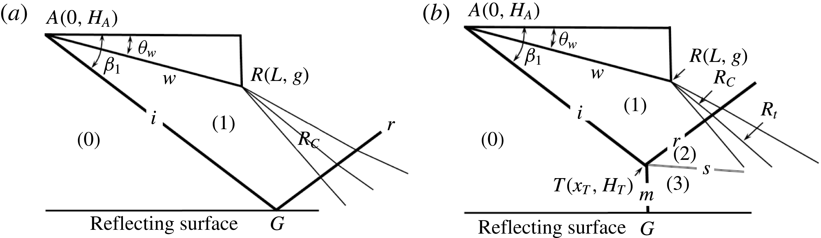
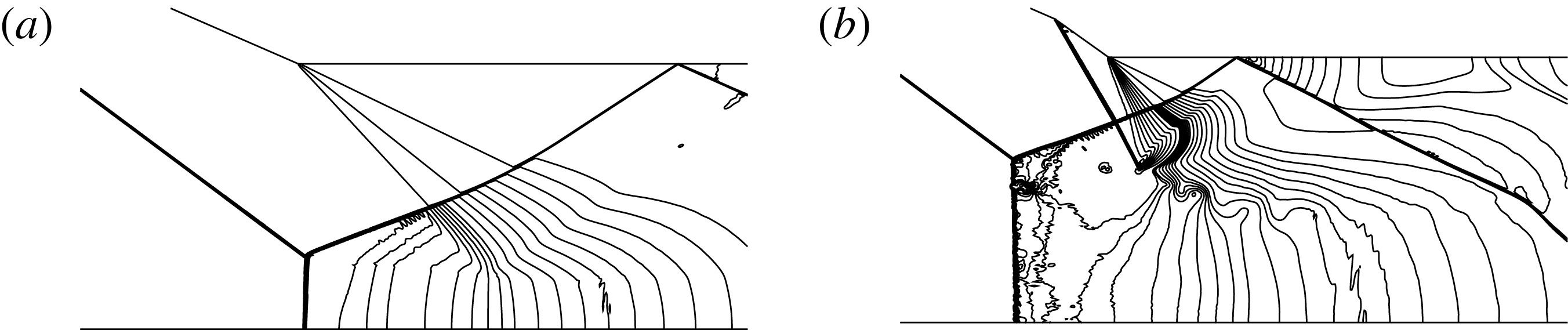
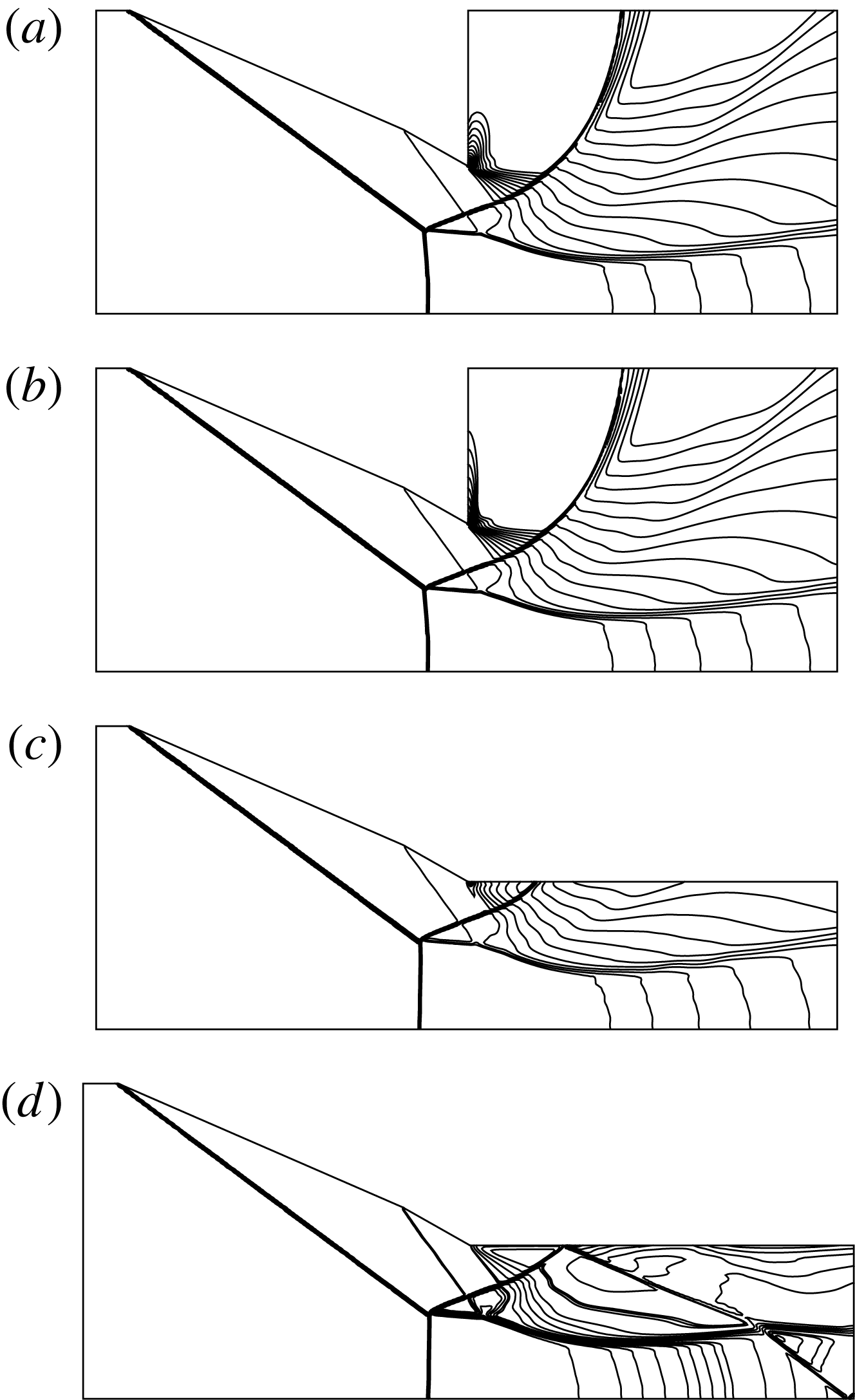
Shock reflection in steady supersonic flow is a well-studied phenomenon (Ben-Dor Reference Ben-Dor2007). As displayed in figure 1, for a supersonic flow with inflow Mach number
 $M_{0}>1$
, a wedge of length
 $w$
and angle
 $\unicode[STIX]{x1D703}_{w}$
induces an incident shock wave (
 $i$
), which reflects from the reflecting surface, leading to either regular reflection (RR) or Mach reflection (MR). For RR, the reflection of the incident shock wave (
 $i$
) produces a reflected shock wave (
 $r$
). For MR, first observed by Mach (Reference Mach1878), the reflection of the incident shock wave (
 $i$
) produces a reflected shock wave (
 $r$
) and a strong shock wave called the Mach stem (
 $m$
). These three shock waves are connected by the triple point (
 $T$
).
A slipline (
 $s$
) is issued from this triple point. This slipline balances the pressures between the flow regions downstream of the reflected shock wave and the Mach stem. The slipline and the reflecting surface enclose a flow region that can be approximately treated as a quasi-one-dimensional duct with averaged flow parameters satisfying quasi-one-dimensional isentropic flow relations (Azevedo & Liu Reference Azevedo and Liu1993; Li & Ben-Dor Reference Li and Ben-Dor1997; Mouton & Hornung Reference Mouton and Hornung2007; Gao & Wu Reference Gao and Wu2010). The transmitted expansion waves (denoted
 $R_{t}$
in figure 1
b) from the trailing edge (
 $R$
) intersect this slipline and reduce the pressure, so that the convergence of the quasi-one-dimensional flow duct slows down to create a sonic throat. The three-shock waves and the slipline separate the flow into four regions (labelled (0), (1), (2) and (3)), the solutions of which in the vicinity of the triple point can be found using the three-shock theory of Von Neumann (Reference Von Neumann1945).
Shock reflection configuration. (a) Regular reflection. (b) Mach reflection.

The criteria for transition to Mach reflection from regular reflection and vice versa have been provided by Von Neumann (Reference Von Neumann1943). In the plane
 $(M_{0},\unicode[STIX]{x1D703}_{w})$
, where
 $M_{0}$
is the free-stream Mach number, there are two curves called the detachment criterion (
 $\unicode[STIX]{x1D703}_{w}=\unicode[STIX]{x1D703}_{w}^{(D)}(M_{0})$
) and von Neumann criterion (
 $\unicode[STIX]{x1D703}_{w}=\unicode[STIX]{x1D703}_{w}^{(N)}(M_{0})$
), with
 $\unicode[STIX]{x1D703}_{w}^{(N)}(M_{0})<\unicode[STIX]{x1D703}_{w}^{(D)}(M_{0})$
. Above the detachment criterion
 $(\unicode[STIX]{x1D703}_{w}>\unicode[STIX]{x1D703}_{w}^{(D)}(M_{0}))$
, only MR is possible. Below the von Neumann criterion
 $(\unicode[STIX]{x1D703}_{w}<\unicode[STIX]{x1D703}_{w}^{(N)}(M_{0}))$
only RR is possible. These two curves enclose a region in the plane
 $(M_{0},\unicode[STIX]{x1D703}_{w})$
called the dual solution domain, within which both reflections may be possible (Henderson & Lozzi Reference Henderson and Lozzi1975; Hornung, Oertel & Sandeman Reference Hornung, Oertel and Sandeman1979), according to theoretical study (Teshukov Reference Teshukov1989; Li & Ben-Dor Reference Li and Ben-Dor1996), numerical study (Vuillon, Zeitoun & Ben-Dor Reference Vuillon, Zeitoun and Ben-Dor1995) and experimental study (Chpoun et al.
Reference Chpoun, Passerel, Li and Ben-Dor1995). If the flow condition comes from variations of
 $(M_{0},\unicode[STIX]{x1D703}_{w})$
from the pure RR domain (below the von Neumann criterion), we have RR in the dual solution domain. If the flow condition comes from variations of
 $(M_{0},\unicode[STIX]{x1D703}_{w})$
from the pure MR domain (above the detachment criterion), we have MR in the dual solution domain. This is called a hysteresis phenomenon in transition, see Ben-Dor et al. (Reference Ben-Dor, Ivanov, Vasilev and Elperin2002) and Hornung (Reference Hornung2014) for a thorough review of important works related to this subject. A RR in the dual solution domain may also transit to MR through some upstream perturbation (Ivanov et al.
Reference Ivanov, Klemenkov, Kudryavtsev, Fomin and Kharitonov1997, Reference Ivanov, Markelov, Kudryavtsev and Gimelshein1998; Ivanov, Kudryavtsev & Khotyanovskii Reference Ivanov, Kudryavtsev and Khotyanovskii2000; Kudryavtsev et al.
Reference Kudryavtsev, Khotyanovsky, Ivanov and Vandromme2002; Li, Gao & Wu Reference Li, Gao and Wu2011).
The size of the Mach stem and the mechanism by which the size of the Mach stem is determined were first studied by Hornung & Robinson (Reference Hornung and Robinson1982) who measured the Mach stem height for a set of inflow conditions and concluded that the relative Mach stem height
 $H_{T}$
should be a function of
 $\unicode[STIX]{x1D6FE}$
(specific heat ratio),
 $M_{0}$
,
 $\unicode[STIX]{x1D703}_{w}$
and
 $g/w$
(
 $g$
is the height of the rear wedge corner and
 $w$
is the length of the wedge lower surface). A number of theoretical models have been built to predict the Mach stem height (Azevedo & Liu Reference Azevedo and Liu1993; Li & Ben-Dor Reference Li and Ben-Dor1997; Mouton & Hornung Reference Mouton and Hornung2007; Gao & Wu Reference Gao and Wu2010; Bai & Wu Reference Bai and Wu2017), through establishing pressure relations below the slipline (using quasi-one-dimensional flow theory) and above the slipline (using pressure relations for Mach waves). The balance between the pressure variation over the slipline (caused by the transmitted expansion waves) and that below the slipline (caused by the convergence and divergence of the quasi-one-dimensional duct) determines a Mach stem height that must meet the sonic throat compatibility condition, i.e. sonic condition occurs at the throat (Bai & Wu Reference Bai and Wu2017). If the sonic throat compatibility condition is not yet met, then a pressure perturbation generated somewhere in the duct propagates towards the Mach stem through the subsonic portion of this duct to adjust the Mach stem height (Li & Ben-Dor Reference Li and Ben-Dor1997).
The previous studies involve only one incident shock wave. Here, we consider shock reflection with two incident shock waves. The second incident shock wave is downstream of the first one and is caused by deflecting further the wedge lower surface at some point. The strength of the second incident shock wave is determined by the additional wedge deflection angle (denoted
 $\unicode[STIX]{x1D6FF}$
).
The reason to consider such a configuration is related to possible application. For instance, the inlet wall of air breathing engines may be allowed to have a double wedge configuration. In fact, Li & Ben-Dor (Reference Li and Ben-Dor1999) have studied unsteady Mach reflection, with a moving shock wave impinging a double wedge. They found that after the shock impinges the second turning point, two triple points form. The shock interaction problem free of the reflecting surface and with two shock waves generated from a double wedge has been studied by Hu et al. (Reference Hu, Gao, Myong, Dou and Khoo2010), Li, Zhu & Luo (Reference Li, Zhu and Luo2014) and Xiong, Zhu & Luo (Reference Xiong, Zhu and Luo2016). Thus, the present study, with a shock reflected over a reflecting surface and in steady supersonic flow, complements the cases studied before.
Apart from the wedge additional deviation, the presence of another shock wave downstream of the incident shock wave may be caused by large downstream pressure and this configuration has been studied by Ben-Dor et al. (Reference Ben-Dor, Elperin, Li and Vasiliev1999), who imposed a downstream pressure behind the wedge rear corner in an artificial way. They found that when this downstream pressure
 $p_{w}$
is larger than
 $p_{1}$
(the pressure in region 1 of figure 1
b, just downstream of the incident shock wave), a shock is generated from the wedge corner. They found two important phenomena: the Mach stem height is increased for
 $p_{w}>p_{1}$
and there is some condition at which inverse-Mach reflection occurs. Since the second incident shock wave studied here also induces a pressure increase, it is interesting to see whether similar phenomena (increase of Mach stem height and advance of transition) occur.
In § 2, a geometrical restriction to have a comparable configuration between the single incident and double incident shock wave cases is given. Numerical computation of flow for shock reflection with two incident shock waves will be provided. Based on the numerical results, a Mach reflection configuration with second incident shock waves is given. We will see that with the influence of the second shock wave, additional shock waves, uniform flow regions and interaction points appear.
In § 3, theoretical models will be provided for determining the solutions in various uniform flow regions and the positions of various interacting points.
In § 4, the Mach stem height model of Bai & Wu (Reference Bai and Wu2017) will be updated to account for the influence of the second incident shock wave on the Mach stem height, for the case where the additional wedge deflection angle is small enough.
In § 5, both theory and computational fluid dynamics (CFD) will be used to study the influence of the second incident shock wave on the flow structure. A relatively coarse grid for CFD will be used in this section to obtain Mach stem height for a large number of cases to see the qualitative influence of the strength of the second incident shock wave.
In § 6, some further considerations will be presented, including a grid refinement study for CFD simulation and a discussion of the reason why theory does not work for very strong second incident shock waves. Preliminary discussions are given for (i) the influence of the second incident shock wave on the advance of transition from regular to Mach reflection to have an inverse-Mach stem, (ii) the influence of the choice of the top boundary downstream of the trailing edge and (iii) the influence of viscosity.
Concluding remarks and suggestion of further studies will be provided in § 7.
2 Mach reflection configuration with two incident shock waves
In this section, we first provide a comparable configuration such that the second incident shock wave is the sole new factor of influence, compared to shock reflection with a single incident shock wave. Then we perform numerical computations to obtain flow structures with single and double incident shock waves. The main flow structures are picked up to form a Mach reflection model with double incident shock waves.
2.1 Geometric restriction for a comparable configuration
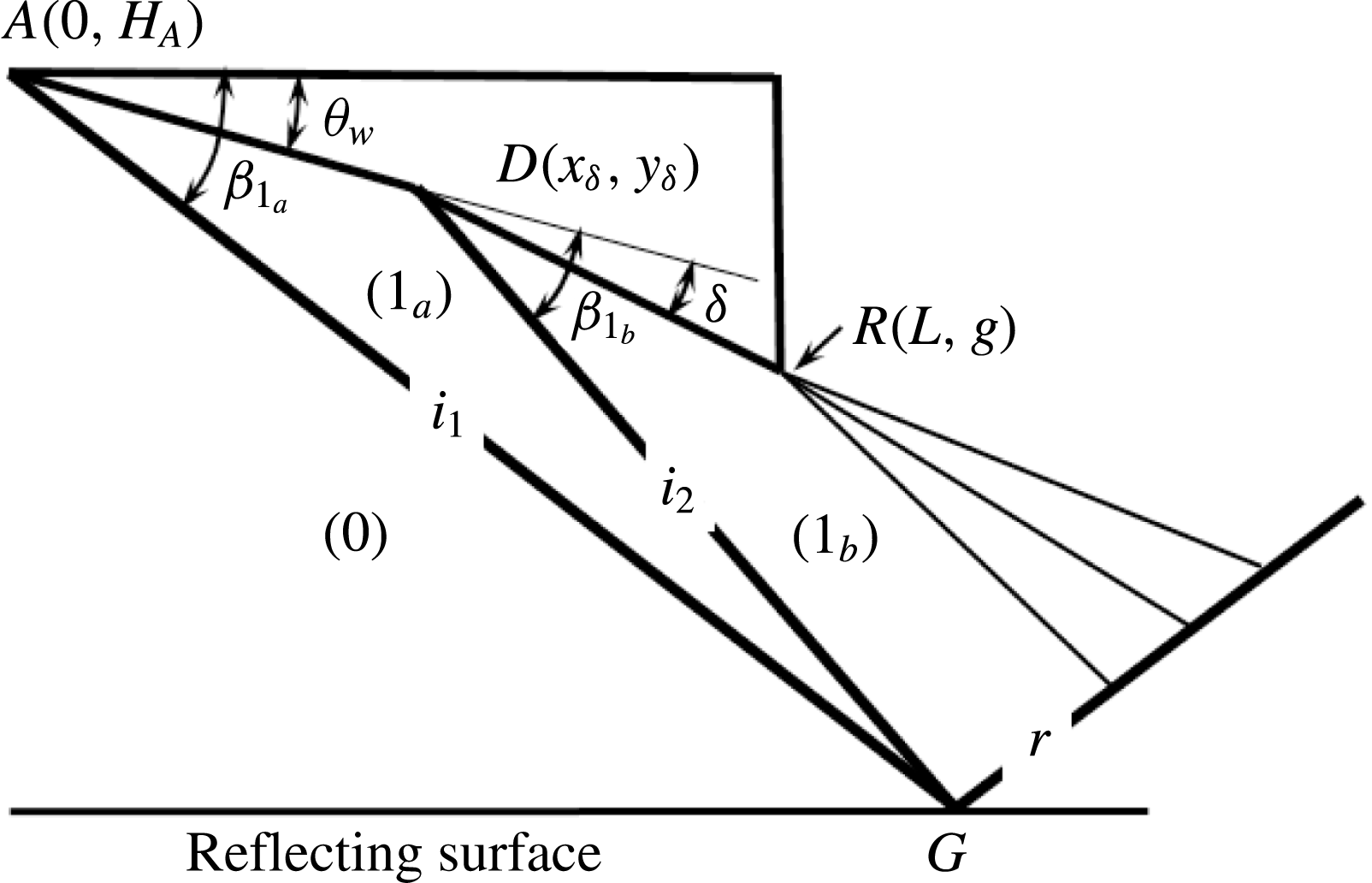
The geometric configuration of shock reflection with two incident shock waves is displayed in figure 2. We adopt a coordinate system with the horizontal axis along the reflecting surface and the vertical axis passing through the leading edge
 $A$
of the wedge. In this coordinate system, the position of
 $A$
is
 $(0,H_{A})$
, where
 $H_{A}$
is the height of the leading edge. The wedge lower surface deflects an additional angle
 $\unicode[STIX]{x1D6FF}$
(called the additional wedge deflection angle) at point
 $D$
, at (
 $x_{\unicode[STIX]{x1D6FF}},y_{_{\unicode[STIX]{x1D6FF}}}$
) to be determined below. The position of
 $D$
will be denoted
 $(x_{D},y_{D})$
in §§ 3 and 4 when another coordinate system is used. The influence of
 $\unicode[STIX]{x1D6FF}$
will be studied for a given wedge angle
 $\unicode[STIX]{x1D703}_{w}$
. The wedge horizontal length is
 $L$
, the wedge rear corner
 $R$
has a height denoted
 $g$
, so that
 $R$
is at
 $(x,y)=(L,g)$
. In the end of this subsection, we will state which parameters are fixed and which are computed from a given
 $\unicode[STIX]{x1D6FF}$
.
The height
 $H_{A}$
can be related to
 $x_{\unicode[STIX]{x1D6FF}}$
,
 $\unicode[STIX]{x1D6FF}$
and other geometrical parameters through the obvious relation
 $$\begin{eqnarray}H_{A}=x_{\unicode[STIX]{x1D6FF}}\tan \unicode[STIX]{x1D703}_{w}+(w\cos \unicode[STIX]{x1D703}_{w}-x_{\unicode[STIX]{x1D6FF}})\tan (\unicode[STIX]{x1D703}_{w}+\unicode[STIX]{x1D6FF})+g.\end{eqnarray}$$
The additional deflection at
 $D$
causes the second incident shock wave. To have a configuration with which we may compare the results with those of shock reflection of a single incident shock wave, we need to place some restrictions on the geometric parameters.
Geometric configuration with an additional wedge deflection angle
 $\unicode[STIX]{x1D6FF}$
, for shock reflection with two incident shock waves. The point
 $D$
at which this additional deflection occurs is chosen such that the two incident shock waves intersect at the reflecting surface in the case of normal reflection.
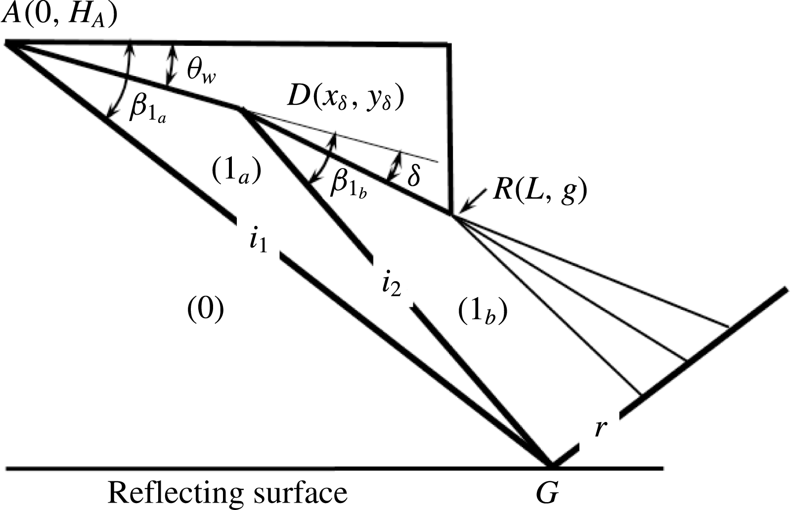
One restriction imposed here is that the two incident shock waves intersect at the reflecting surface. Equating the positions of these two shock waves on the reflecting surface gives
 $$\begin{eqnarray}\frac{H_{A}}{\tan \unicode[STIX]{x1D6FD}_{1_{a}}}=x_{\unicode[STIX]{x1D6FF}}+\frac{H_{A}-x_{\unicode[STIX]{x1D6FF}}\tan \unicode[STIX]{x1D703}_{w}}{\tan (\unicode[STIX]{x1D6FD}_{1_{b}}+\unicode[STIX]{x1D703}_{w})}.\end{eqnarray}$$
Here,
 $\unicode[STIX]{x1D6FD}_{1_{a}}$
is the shock angle of the first incident shock wave and
 $\unicode[STIX]{x1D6FD}_{1_{b}}$
is the shock angle of the second incident shock wave.
The expressions (2.1) and (2.2) can be solved to give
 $$\begin{eqnarray}x_{\unicode[STIX]{x1D6FF}}={\displaystyle \frac{g+L\tan (\unicode[STIX]{x1D6FF}+\unicode[STIX]{x1D703}_{w})}{\tan (\unicode[STIX]{x1D6FF}+\unicode[STIX]{x1D703}_{w})-\tan \unicode[STIX]{x1D703}_{w}+{\displaystyle \frac{\tan \unicode[STIX]{x1D6FD}_{1_{a}}(\tan (\unicode[STIX]{x1D6FD}_{1_{b}}+\unicode[STIX]{x1D703}_{w})-\tan \unicode[STIX]{x1D703}_{w})}{\tan (\unicode[STIX]{x1D6FD}_{1_{b}}+\unicode[STIX]{x1D703}_{w})-\tan \unicode[STIX]{x1D6FD}_{1_{a}}}}}}\end{eqnarray}$$
and
 $$\begin{eqnarray}H_{A}=x_{\unicode[STIX]{x1D6FF}}\frac{\tan \unicode[STIX]{x1D6FD}_{1_{a}}\tan (\unicode[STIX]{x1D6FD}_{1_{b}}+\unicode[STIX]{x1D703}_{w})-\tan \unicode[STIX]{x1D703}_{w}\tan \unicode[STIX]{x1D6FD}_{1_{a}}}{\tan (\unicode[STIX]{x1D6FD}_{1_{b}}+\unicode[STIX]{x1D703}_{w})-\tan \unicode[STIX]{x1D6FD}_{1_{a}}}.\end{eqnarray}$$
Another restriction is to make the influence of the second shock wave on the Mach stem height be solely determined by
 $\unicode[STIX]{x1D6FF}$
. Hornung & Robinson (Reference Hornung and Robinson1982) pointed out that, for standard Mach reflection, the Mach stem height
 $H_{T}$
should vary according to
 $$\begin{eqnarray}\frac{H_{T}}{L}=f\left(\unicode[STIX]{x1D6FE},M_{0},\unicode[STIX]{x1D703}_{w},\frac{g}{L}\right).\end{eqnarray}$$
Once the second incident shock wave appears, equation (2.5) naturally becomes
 $$\begin{eqnarray}\frac{H_{T}}{L}=f\left(\unicode[STIX]{x1D6FE},M_{0},\unicode[STIX]{x1D703}_{w},\frac{g}{L},\unicode[STIX]{x1D6FF}\right).\end{eqnarray}$$
Thus, the ratio
 $g/L$
should fixed here to be independent on
 $\unicode[STIX]{x1D6FF}$
, in order that
 $\unicode[STIX]{x1D6FF}$
becomes the sole parameter to account for the influence of the second incident shock wave.
In summary, to study the sole influence of the second incident shock wave in terms of the wedge deflection angle
 $\unicode[STIX]{x1D6FF}$
, we fix
 $M_{0},\unicode[STIX]{x1D703}_{w},L$
and
 $g$
to be independent of
 $\unicode[STIX]{x1D6FF}$
, for any given
 $\unicode[STIX]{x1D6FF}$
. The horizontal location
 $x_{\unicode[STIX]{x1D6FF}}$
of point
 $D$
is determined from (2.3) and the inlet height
 $H_{A}$
is set to the value given by (2.4).
Then, with such restrictions, the two incident shock waves intersect at the reflecting surface in the case of normal reflection. Moreover, with
 $M_{0},\unicode[STIX]{x1D703}_{w},L$
and
 $g$
fixed, the influence of the second incident shock wave or
 $\unicode[STIX]{x1D6FF}$
can be isolated according to (2.6).
The study of the influence of a second incident shock wave without the present geometric restrictions will be considered in the future when the issue of transition is to be studied.
2.2 Typical flow structures by numerical simulation
Here we demonstrate some numerical solutions in order to construct the flow model in § 2.3. For this computation, we use the second-order Roe scheme based on an unstructured grid, using an unstructured grid with approximately 460 cells along the streamwise direction and 180 cells along the transverse direction. In § 6 we will demonstrate a comparison of results between such a grid and a more refined grid, to show that the use of the present grid is suitable. The purpose of this paper is to study the Mach reflection configuration. Once the flow condition is in the dual solution domain, we compute the flow in such a way as to obtain Mach reflection. This is done here by computing an initial flow at a lower Mach number (low enough so that the reflection of the first incident shock wave is in the MR condition) to have Mach reflection and then using this as initial data to recompute the flow with the final Mach number in the inlet.
There is some flexibility to consider the upper boundary downstream of the trailing edge. In applications, it may be a solid wall or an open boundary (that can be treated as a non-reflecting boundary). We consider this boundary as a solid wall and a comparison of different treatments is given in § 6.2.
After some numerical computation for various choices of parameters, we find that (i) the flow structure is altered by the second incident shock wave in the dual solution domain of the first incident shock wave, and (ii) inverse-Mach reflection is triggered below the von Neumann condition of the first incident shock wave. Now we present these results for two typical flow conditions.
(i) The reflection of the first incident shock wave is in dual solution domain. This occurs for instance when
 $M_{0}=3.98$
,
$\unicode[STIX]{x1D703}_{w}=23.5^{\circ }$
and
$g\cos \unicode[STIX]{x1D703}_{w}/L=0.4$
. In this case,
$\unicode[STIX]{x1D703}_{w}>\unicode[STIX]{x1D703}_{w}^{(N)}(M_{0})$
(dual solution domain). Even when
$\unicode[STIX]{x1D6FF}=0^{\circ }$
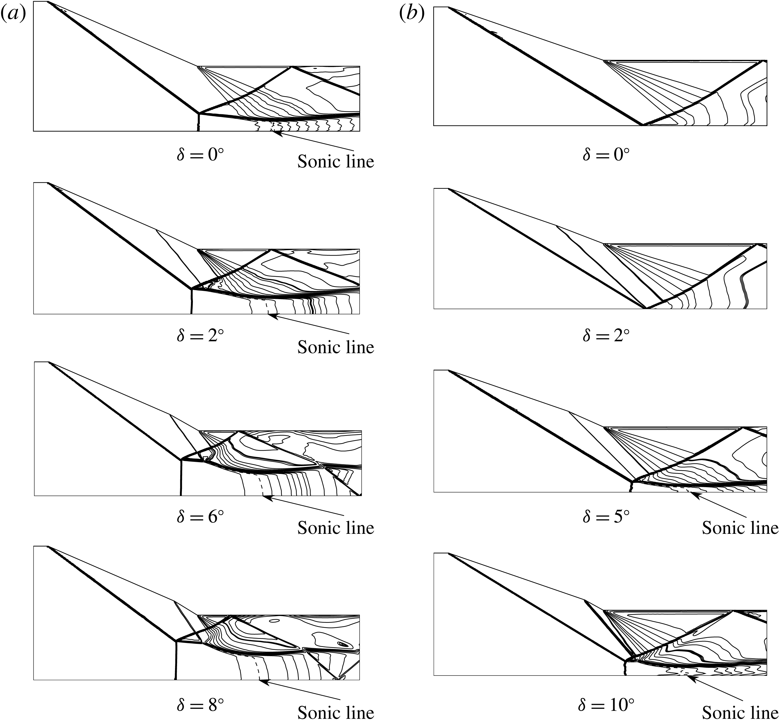
, we may have Mach reflection. For this typical condition, we have computed the flow with
$\unicode[STIX]{x1D6FF}=0^{\circ }$
,
$2^{\circ }$
,
$6^{\circ }$
,
$8^{\circ }$
. The Mach contours are displayed in figure 3(a). Compared to the flow with single incident shock wave (
$\unicode[STIX]{x1D6FF}=0^{\circ }$
), the Mach stem height is higher for
$\unicode[STIX]{x1D6FF}>0^{\circ }$
and increases with
$\unicode[STIX]{x1D6FF}$
. The slipline suddenly alters its direction at some point downstream of the triple point: it deflects more towards the reflecting surface when
$\unicode[STIX]{x1D6FF}$
is high.
(ii) The reflection of the first incident shock wave is below the von Neumann condition. This occurs for instance when
$M_{0}=3.98$
,
$\unicode[STIX]{x1D703}_{w}=19^{\circ }$
and
$g\cos \unicode[STIX]{x1D703}_{w}/L=0.4$
. In this case,
$\unicode[STIX]{x1D703}_{w}<\unicode[STIX]{x1D703}_{w}^{(N)}(M_{0})$
so that regular reflection occurs for
$\unicode[STIX]{x1D6FF}=0^{\circ }$
. For this typical condition, we computed the flow with
$\unicode[STIX]{x1D6FF}=0^{\circ }$
,
$2^{\circ }$
,
$5^{\circ }$
,
$10^{\circ }$
. The Mach contours are displayed in figure 3(b). At
$\unicode[STIX]{x1D6FF}=2^{\circ }$
we still have regular reflection. Mach reflection occurs at
$\unicode[STIX]{x1D6FF}=5^{\circ }$
and
$10^{\circ }$
. This means that the second incident shock wave induces Mach reflection of the first incident shock wave. The flow structure is similar to case (i) for
$\unicode[STIX]{x1D6FF}>0^{\circ }$
, but with inversion of the Mach stem and with the initial part of the slipline deflecting upward. This inverted Mach reflection phenomenon has also been observed by Ben-Dor et al. (Reference Ben-Dor, Elperin, Li and Vasiliev1999) with high downstream pressure.


Mach number contours with single and double incident shock waves for various
 $\unicode[STIX]{x1D6FF}$
. (a)
 $M_{0}=3.98$
,
 $\unicode[STIX]{x1D703}_{w}=23.5^{\circ }$
. (b)
 $M_{0}=3.98$
,
 $\unicode[STIX]{x1D703}_{w}=19^{\circ }$
.

2.3 Overall configuration for Mach reflection
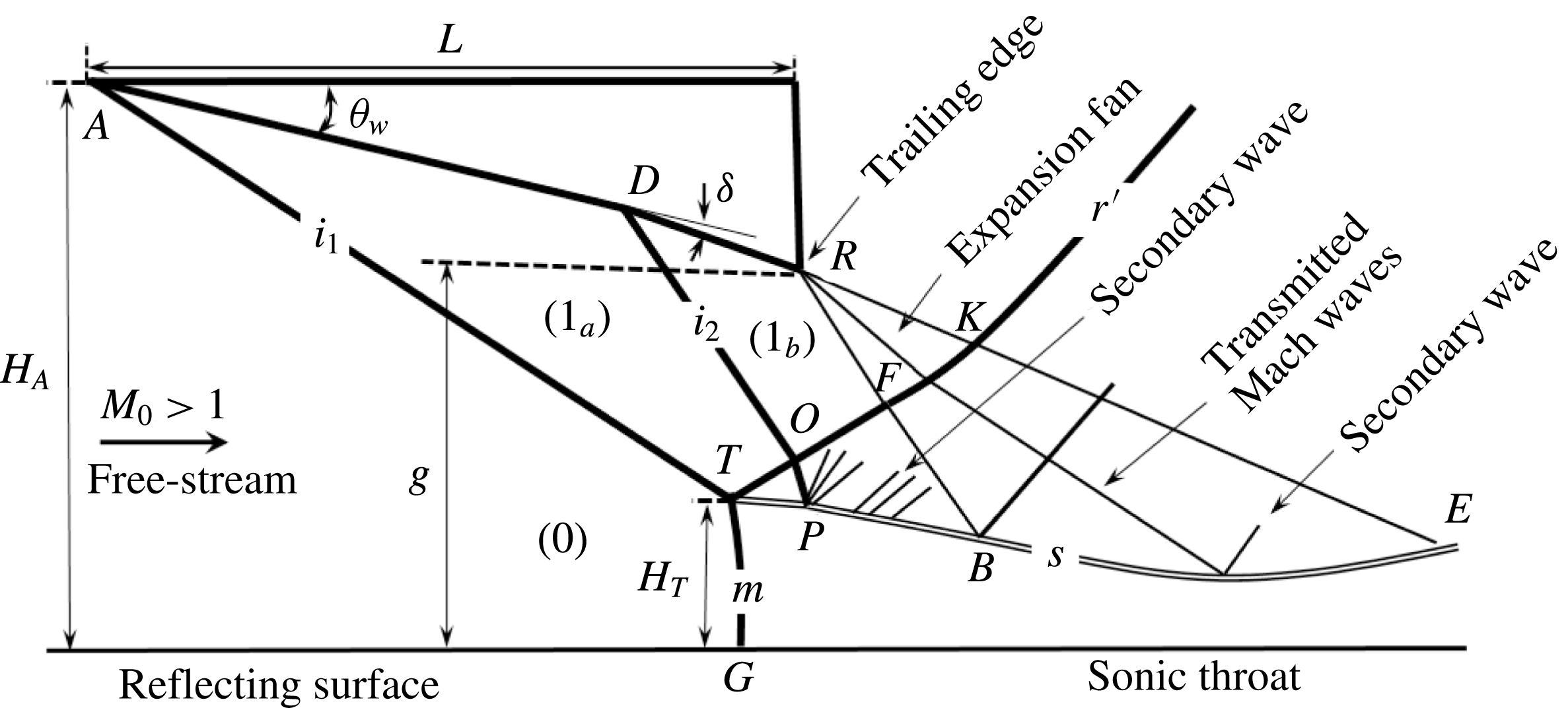
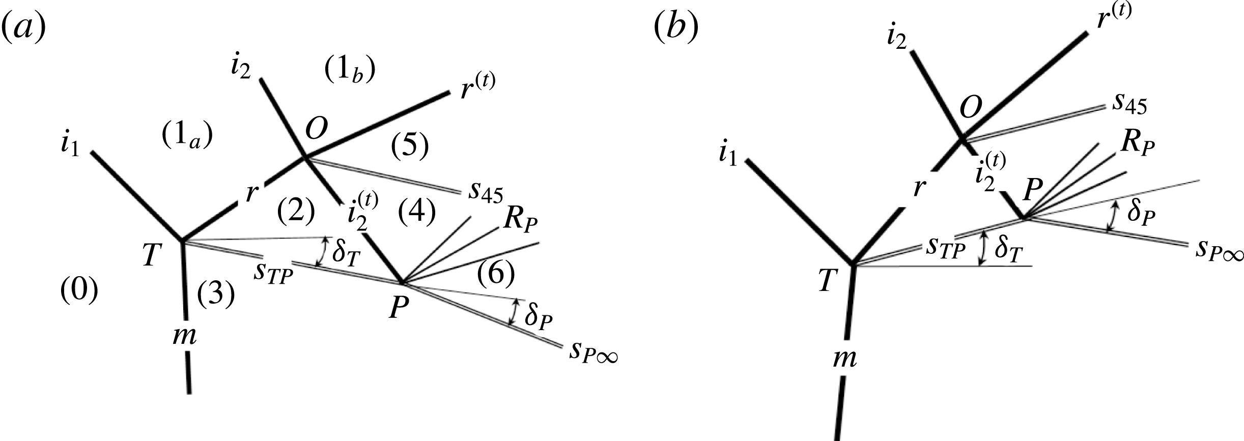
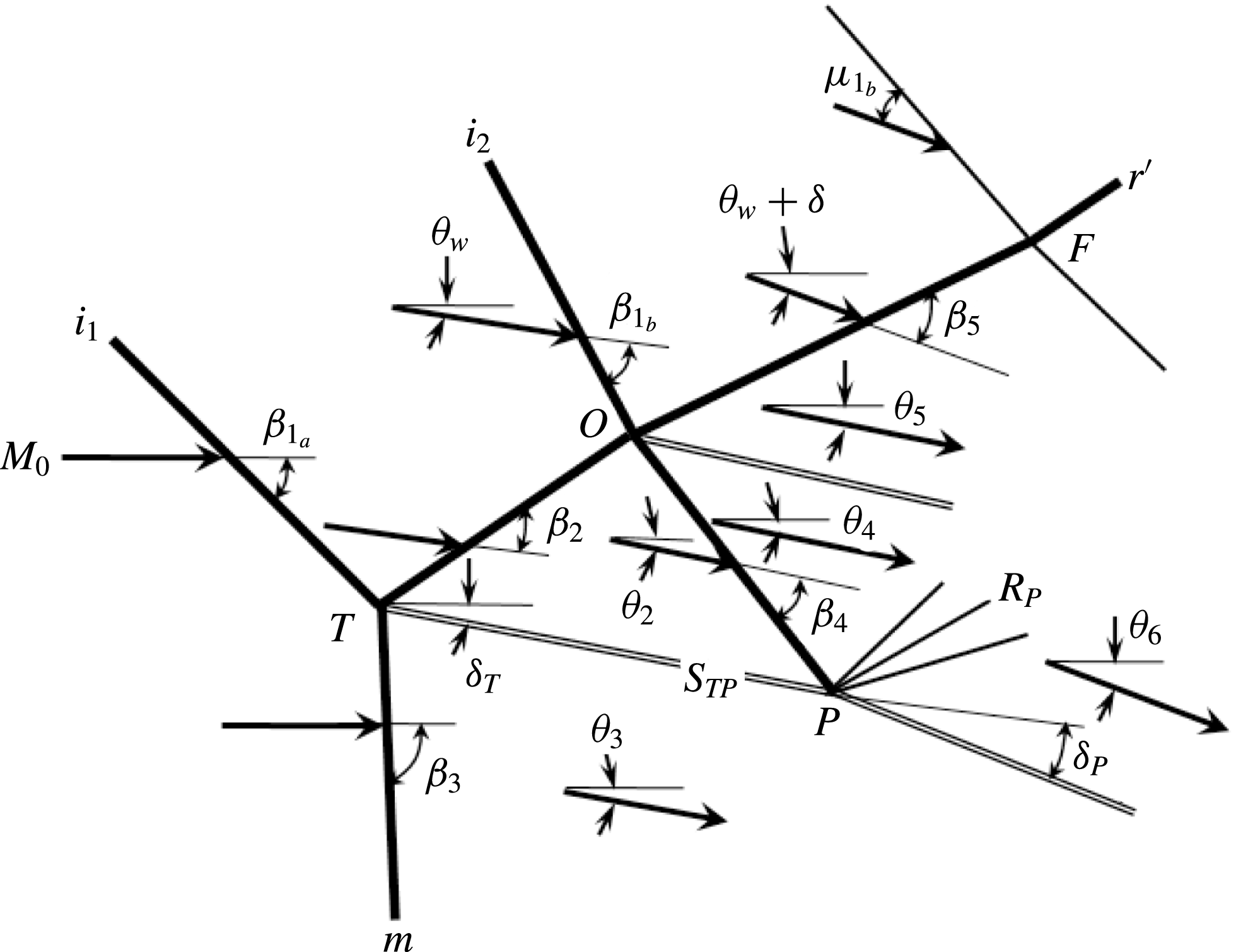
The overall configuration for Mach reflection follows from the numerical solutions presented above. The flow structure in the case of Mach reflection with influence of the second incident shock wave is schematically displayed in figure 4 for a global view. For a local view with a distinction between direct and inverse-Mach stems, see figure 5.
The two incident shock waves are labelled with
 $i_{1}$
(first) and
 $i_{2}$
(second), the reflected shock wave of the first incident shock wave is labelled
 $r$
. The second incident shock wave
 $i_{2}$
and the reflected shock wave interact at point
 $O$
. This interaction produces transmitted shock waves
 $r^{(t)}$
and
 $i_{2}^{(t)}$
, which are separated by a new slipline
 $s_{45}$
(figure 5). The reflection of the transmitted shock wave
 $i_{2}^{(t)}$
on the slipline produces reflected expansion waves
 $R_{P}$
at the point
 $P$
(reflection point on the slipline).
The various waves divide the flow into eight regions labelled
 $j=0,1_{a},1_{b},2,3,4,5,6$
as displayed in figures 4 and 5(a).
Configuration of flow structure for Mach reflection with two incident shock waves.

Configuration of flow structure near the interaction zones. (a) Mach reflection with
 $\unicode[STIX]{x1D703}_{w}>\unicode[STIX]{x1D703}_{w}^{(N)}(M_{0})$
, (b) Mach reflection with
 $\unicode[STIX]{x1D703}_{w}<\unicode[STIX]{x1D703}_{w}^{(N)}(M_{0})$
.

3 Exact solutions in uniform flow regions and interacting points
In this section, expressions for determining uniform flow solutions of various shock waves and the interaction points of the shock waves will be provided. The treatment of curved shock wave and slipline due to interaction from Mach waves will be discussed in § 4.
3.1 Model of uniform flow solutions
The various flow regions and interacting points are defined in figures 4 and 5(a). The uniform flow solutions rely on the use of shock relation and Prandtl–Meyer wave relation. To abbreviate the expressions, we have
 $$\begin{eqnarray}\left.\begin{array}{@{}c@{}}f_{\unicode[STIX]{x1D703}}(M,\unicode[STIX]{x1D6FD})={\displaystyle \frac{2(M^{2}\sin ^{2}\unicode[STIX]{x1D6FD}-1)}{(M^{2}(\unicode[STIX]{x1D6FE}+\cos 2\unicode[STIX]{x1D6FD})+2)\tan \unicode[STIX]{x1D6FD}}},\\ f_{M}(M,\unicode[STIX]{x1D6FD})=\sqrt{{\displaystyle \frac{(\unicode[STIX]{x1D6FE}-1)M^{2}+2}{2\unicode[STIX]{x1D6FE}M^{2}\sin ^{2}\unicode[STIX]{x1D6FD}-(\unicode[STIX]{x1D6FE}-1)}}+{\displaystyle \frac{2M^{2}\cos ^{2}\unicode[STIX]{x1D6FD}}{(\unicode[STIX]{x1D6FE}-1)M^{2}\sin ^{2}\unicode[STIX]{x1D6FD}+2}}},\\ f_{p}(M,\unicode[STIX]{x1D6FD})=1+{\displaystyle \frac{2\unicode[STIX]{x1D6FE}}{\unicode[STIX]{x1D6FE}+1}}(M^{2}\sin ^{2}\unicode[STIX]{x1D6FD}-1)\end{array}\right\}\end{eqnarray}$$
for the shock angle relation, Mach number relation and pressure relation, where
 $\unicode[STIX]{x1D6FD}$
is the shock angle. We also have
 $$\begin{eqnarray}\left.\begin{array}{@{}c@{}}\unicode[STIX]{x1D708}(M)=\sqrt{{\displaystyle \frac{\unicode[STIX]{x1D6FE}+1}{\unicode[STIX]{x1D6FE}-1}}}\arctan \sqrt{{\displaystyle \frac{\unicode[STIX]{x1D6FE}-1}{\unicode[STIX]{x1D6FE}+1}}(M^{2}-1)}-\arctan \sqrt{M^{2}-1},\\ \unicode[STIX]{x1D717}(M)=1+{\displaystyle \frac{\unicode[STIX]{x1D6FE}-1}{2}}M^{2},\end{array}\right\}\end{eqnarray}$$
where
 $\unicode[STIX]{x1D708}(M)$
is the Prandtl–Meyer function and the factor
 $\unicode[STIX]{x1D717}(M)$
usually appears in isentropic relations.
The solutions in region
 $j=0$
are uniform and given. The solutions in
 $1_{a}$
and
 $1_{b}$
are also uniform and are given by the standard oblique shock wave solutions. These solutions give the shock angles
 $\unicode[STIX]{x1D6FD}_{1_{a}}$
and
 $\unicode[STIX]{x1D6FD}_{1_{b}}$
for the two incident shock waves, flow parameters
 $p_{1_{a}},M_{1_{a}}$
in region
 $1_{a}$
and flow parameters
 $p_{1_{b}},M_{1_{b}}$
in region
 $1_{b}$
.
Compared to single incident shock wave, where we have only one triple point ahead of the expansion waves, here we have three interaction points
 $T,O$
and
 $P$
, as shown in figures 4 and 5.
Similar to the triple point solution of Von Neumann (Reference Von Neumann1945), here, the flow solutions in regions in the vicinity of the interaction points
 $T,O$
and
 $P$
are taken to be uniform flow solutions, ignoring the influence of secondary waves in region 2 (this influence will be considered in the Mach stem height model studied in § 4).
3.1.1 Triple point solution for both direct and inverse-Mach reflection
The solution of uniform regions near the triple point
 $T$
is independent of the second incident shock wave and is apparently the same as for standard (direct) Mach reflection. For standard Mach reflection, this solution is given by the three-shock theory of Von Neumann (Reference Von Neumann1945) which gives a slipline angle
 $\unicode[STIX]{x1D6FF}_{T}>0$
. However, for the present study, inverse-Mach reflection may be possible so that the slipline angle may take
 $\unicode[STIX]{x1D6FF}_{T}<0$
.
Now we outline the three-shock theory. It gives the flow parameters in the regions
 $1_{a}$
, 2 and 3 in the vicinity of the triple point (see figures 4 and 5), including the initial angle
 $\unicode[STIX]{x1D6FF}_{T}=\unicode[STIX]{x1D703}_{2}(T)$
of the slipline and the initial angle
 $\unicode[STIX]{x1D6FD}_{T}=\unicode[STIX]{x1D6FD}_{2}(T)$
of the reflected shock wave. More details on shock and deflection angles in various regions are shown in figure 6.
Deflection angles and shock angles in various regions.

The shock angle
 $\unicode[STIX]{x1D6FD}_{1_{a}}$
of the first incident shock wave and the flow parameters (
 $M_{1_{a}},p_{1_{a}}$
) are related to the upstream condition
 $(M_{0},p_{0})$
and the wedge angle
 $\unicode[STIX]{x1D703}_{w}$
through the oblique shock wave relations
 $$\begin{eqnarray}\tan \unicode[STIX]{x1D703}_{w}=f_{\unicode[STIX]{x1D703}}(M_{0},\unicode[STIX]{x1D6FD}_{1_{a}}),\quad M_{1_{a}}=f_{M}(M_{0},\unicode[STIX]{x1D6FD}_{1_{a}}),\quad p_{1_{a}}=p_{0}f_{p}(M_{0},\unicode[STIX]{x1D6FD}_{1_{a}}).\end{eqnarray}$$
The oblique shock wave relation for flow parameters in regions 2 and 3 are
 $$\begin{eqnarray}\tan (\unicode[STIX]{x1D703}_{w}-\unicode[STIX]{x1D703}_{2})=f_{\unicode[STIX]{x1D703}}(M_{1_{a}},\unicode[STIX]{x1D6FD}_{2}),\quad M_{2}=f_{M}(M_{1_{a}},\unicode[STIX]{x1D6FD}_{2}),\quad p_{2}=p_{1_{a}}f_{p}(M_{1_{a}},\unicode[STIX]{x1D6FD}_{2})\end{eqnarray}$$
and
 $$\begin{eqnarray}\tan \unicode[STIX]{x1D703}_{3}=f_{\unicode[STIX]{x1D703}}(M_{0},\unicode[STIX]{x1D6FD}_{3}),\quad M_{3}=f_{M}(M_{0},\unicode[STIX]{x1D6FD}_{3}),\quad p_{3}=p_{0}f_{p}(M_{0},\unicode[STIX]{x1D6FD}_{3}),\end{eqnarray}$$
where
 $\unicode[STIX]{x1D6FD}_{2}$
is the shock angle for the reflected shock wave
 $r$
and
 $\unicode[STIX]{x1D6FD}_{3}$
is the shock angle of Mach stem near the triple point. Both (3.3) and (3.4) are solved as weak shock waves while a strong shock wave solution is solved for (3.5).
Since on both sides of slipline the pressures and the flow directions are the same, the following additional relations hold
 $$\begin{eqnarray}\unicode[STIX]{x1D703}_{2}=\unicode[STIX]{x1D703}_{3},\quad p_{2}=p_{3}.\end{eqnarray}$$
The slipline has the deflection angle near the triple point given by
 $\unicode[STIX]{x1D6FF}_{T}=\unicode[STIX]{x1D703}_{2}$
.
Note that, in the case of inverse-Mach reflection for
 $\unicode[STIX]{x1D703}_{w}<\unicode[STIX]{x1D703}_{w}^{(N)}$
,
 $\unicode[STIX]{x1D703}_{2}$
is allowed to have negative value. For direct Mach reflection,
 $\unicode[STIX]{x1D703}_{2}>0$
.
3.1.2 Shock interaction solution at point
$O$

As shown in figure 5, the second incident shock wave (
 $i_{2}$
) and the reflected shock wave (
 $r$
) intersect at point
 $O$
to produce a shock–shock interaction, leading to two transmitted shock waves
 $r^{(t)}$
,
 $i_{2}^{(t)}$
and a slipline
 $s_{45}$
. This slipline separates the flow behind the transmitted shock waves into regions 4 and 5, assumed uniform in the present model.
The flow in region 2 upstream of the transmitted shock wave
 $i_{2}^{(t)}$
has been given by the triple point three-shock theory. For flow in region
 $1_{b}$
upstream of
 $r^{(t)}$
, the oblique shock wave relation gives
 $$\begin{eqnarray}\tan \unicode[STIX]{x1D6FF}=f_{\unicode[STIX]{x1D703}}(M_{1_{a}},\unicode[STIX]{x1D6FD}_{1_{b}}),\quad M_{1_{b}}=f_{M}(M_{1_{a}},\unicode[STIX]{x1D6FD}_{1_{b}}),\quad p_{1_{b}}=p_{1_{a}}f_{p}(M_{1_{a}},\unicode[STIX]{x1D6FD}_{1_{b}}),\end{eqnarray}$$
where
 $\unicode[STIX]{x1D6FD}_{1_{b}}$
is the shock angle of the second incident shock wave.
Applying the oblique shock wave relations to shock
 $r^{(t)}$
(with shock angle
 $\unicode[STIX]{x1D6FD}_{5}$
) and
 $i_{2}^{(t)}$
(with shock angle
 $\unicode[STIX]{x1D6FD}_{4}$
) gives
 $$\begin{eqnarray}\tan (\unicode[STIX]{x1D703}_{w}+\unicode[STIX]{x1D6FF}-\unicode[STIX]{x1D703}_{5})=f_{\unicode[STIX]{x1D703}}(M_{1_{b}},\unicode[STIX]{x1D6FD}_{5}),\quad M_{5}=f_{M}(M_{1_{b}},\unicode[STIX]{x1D6FD}_{5}),\quad p_{5}=p_{1_{b}}f_{p}(M_{1_{b}},\unicode[STIX]{x1D6FD}_{5})\end{eqnarray}$$
and
 $$\begin{eqnarray}\tan (\unicode[STIX]{x1D703}_{2}-\unicode[STIX]{x1D703}_{4})=f_{\unicode[STIX]{x1D703}}(M_{2},\unicode[STIX]{x1D6FD}_{4}),\quad M_{4}=f_{M}(M_{2},\unicode[STIX]{x1D6FD}_{4}),\quad p_{4}=p_{2}f_{p}(M_{2},\unicode[STIX]{x1D6FD}_{4}).\end{eqnarray}$$
Since the pressure and flow directions are the same across a slipline, we have two addition expressions
 $$\begin{eqnarray}\unicode[STIX]{x1D703}_{4}=\unicode[STIX]{x1D703}_{5},\quad p_{4}=p_{5}.\end{eqnarray}$$
3.1.3 Shock/slipline reflection solution at point
$P$

The transmitted second incident shock wave
 $i_{2}^{(t)}$
intersects the slipline at point
 $P$
, see figure 5 for details. The pressure jumps from
 $p_{2}$
to
 $p_{4}$
(with
 $p_{4}>p_{2}$
) across the shock wave
 $i_{2}^{(t)}$
. The pressure above the slipline should be the same as the pressure below the slipline. However, the subsonic flow below the slipline cannot sustain such a pressure jump. Thus, at the reflection, there must be an expansion fan to reduce the pressure, so that the pressure at region 6 (near
 $P$
) equals
 $p_{2}$
. Such a pressure drop is possible only if the slipline deflects an additional angle
 $\unicode[STIX]{x1D6FF}_{P}$
, with
 $\unicode[STIX]{x1D6FF}_{P}$
connected to the pressure drop
 $p_{6}-p_{4}=p_{2}-p_{4}$
by the Prandtl–Meyer relation
 $$\begin{eqnarray}\displaystyle \left.\begin{array}{@{}c@{}}p_{6}=p_{4}\left({\displaystyle \frac{1+{\displaystyle \frac{\unicode[STIX]{x1D6FE}-1}{2}}M_{4}^{2}}{1+{\displaystyle \frac{\unicode[STIX]{x1D6FE}-1}{2}}M_{6}^{2}}}\right)^{\unicode[STIX]{x1D6FE}/(\unicode[STIX]{x1D6FE}-1)},\\ \unicode[STIX]{x1D708}(M_{6})-\unicode[STIX]{x1D708}(M_{4})=\unicode[STIX]{x1D6FF}_{P}+\unicode[STIX]{x1D703}_{2}-\unicode[STIX]{x1D703}_{4},\\ p_{6}=p_{2}.\end{array}\right\} & & \displaystyle\end{eqnarray}$$
The triple point solution provides
 $\unicode[STIX]{x1D703}_{2},p_{2}$
and the shock/shock interaction solution (at point
 $O$
) provides
 $p_{4}$
and
 $\unicode[STIX]{x1D703}_{4}$
, thus the expressions (3.11) and (3.2) can be used to obtain
 $\unicode[STIX]{x1D6FF}_{P}$
. Obviously,
 $\unicode[STIX]{x1D6FF}_{P}$
is a function of
 $\unicode[STIX]{x1D6FF}$
, i.e.
 $\unicode[STIX]{x1D6FF}_{P}=\unicode[STIX]{x1D6FF}_{P}(\unicode[STIX]{x1D6FF})$
, with
 $\unicode[STIX]{x1D6FF}_{P}(0)=0$
.
3.2 Positions of various geometric and interaction points
We choose a coordinate system such that the
 $x$
axis is along the reflecting surface and the
 $y$
axis passes the triple point. The triple point is thus located at
 $$\begin{eqnarray}x_{T}=0,\quad y_{T}=H_{T}.\end{eqnarray}$$
This is different to what we have used in § 2.1. Actually, the Mach stem height
 $H_{T}$
is guessed and its final value will be solved using the algorithm detailed in § 5.
3.2.1 Relations for positions of points
$R$
,
$A$
and
$D$


The position of the trailing edge
 $R$
is given by
 $$\begin{eqnarray}x_{R}=L-(H_{A}-H_{T})\cot \unicode[STIX]{x1D6FD}_{1_{a}},\quad y_{R}=g,\end{eqnarray}$$
where
 $H_{A}$
is the inlet height given by (2.4). See § 2.1 for restrictions on the geometry. Point
 $A$
is at (
 $x_{A},y_{A}$
) with
 $$\begin{eqnarray}x_{A}=-(H_{A}-H_{T})\cot \unicode[STIX]{x1D6FD}_{1_{a}},\quad y_{A}=H_{A}.\end{eqnarray}$$
The position of point
 $D$
(point of generation of the second incident shock wave) is
 $$\begin{eqnarray}x_{D}=x_{\unicode[STIX]{x1D6FF}}+x_{A},\quad y_{D}=y_{A}-(x_{D}-x_{A})\tan \unicode[STIX]{x1D703}_{w},\end{eqnarray}$$
where
 $x_{\unicode[STIX]{x1D6FF}}$
is given by (2.3).
3.2.2 Relations of positions for points
$O,P$
and
$F$


The point
 $O$
lies on both the second incident shock wave (of shock angle
 $\unicode[STIX]{x1D6FD}_{1_{b}}$
and with upstream flow deflection angle
 $\unicode[STIX]{x1D703}_{w}$
) and the reflected shock wave (of shock angle
 $\unicode[STIX]{x1D6FD}_{2}$
and with upstream flow deflection angle
 $\unicode[STIX]{x1D703}_{w}$
), hence
 $$\begin{eqnarray}\left.\begin{array}{@{}c@{}}y_{O}=y_{D}-(x_{O}-x_{D})\tan (\unicode[STIX]{x1D6FD}_{1_{b}}+\unicode[STIX]{x1D703}_{w}),\\ y_{O}=y_{T}+(x_{O}-x_{T})\tan (\unicode[STIX]{x1D6FD}_{2}-\unicode[STIX]{x1D703}_{w}).\end{array}\right\}\end{eqnarray}$$
The point
 $P$
lies on both the first segment
 $s_{TP}$
of the slipline (of deflection angle
 $\unicode[STIX]{x1D6FF}_{T}$
) and the transmitted shock wave
 $i_{2}^{(t)}$
(of shock angle
 $\unicode[STIX]{x1D6FD}_{4}$
and upstream deflection angle
 $\unicode[STIX]{x1D703}_{2}=\unicode[STIX]{x1D6FF}_{T}$
), hence
 $$\begin{eqnarray}\left.\begin{array}{@{}c@{}}y_{P}=y_{T}-(x_{P}-x_{T})\tan \unicode[STIX]{x1D6FF}_{T},\\ y_{P}=y_{O}-(x_{P}-x_{O})\tan (\unicode[STIX]{x1D6FD}_{4}+\unicode[STIX]{x1D703}_{2}).\end{array}\right\}\end{eqnarray}$$
The first characteristic
 $RF$
of the wedge expansion fan (with upstream flow deflection angle
 $\unicode[STIX]{x1D703}_{w}+\unicode[STIX]{x1D6FF}$
) intersects the transmitted reflected shock wave
 $r^{(t)}$
(with shock angle
 $\unicode[STIX]{x1D6FD}_{5}$
and with upstream flow deflection angle
 $\unicode[STIX]{x1D703}_{w}+\unicode[STIX]{x1D6FF}$
) at point
 $F$
. The shock segment
 $OF$
is assumed to be straight, so that the position
 $(x_{F},y_{F})$
(which lies on both the first characteristics
 $RF$
and the shock
 $OF$
) can be evaluated by
 $$\begin{eqnarray}\left.\begin{array}{@{}c@{}}y_{F}=y_{R}-(x_{F}-x_{R})\tan (\unicode[STIX]{x1D707}_{1_{b}}+\unicode[STIX]{x1D703}_{w}+\unicode[STIX]{x1D6FF}),\\ y_{F}=y_{O}+(x_{F}-x_{O})\tan (\unicode[STIX]{x1D6FD}_{5}-\unicode[STIX]{x1D703}_{w}-\unicode[STIX]{x1D6FF}).\end{array}\right\}\end{eqnarray}$$
Here
 $\unicode[STIX]{x1D707}_{1_{b}}=\arcsin (1/M_{1_{b}})$
is the Mach angle in region
 $1_{b}$
.
3.2.3 Explicit expressions for the positions of various points
With the positions
 $T,R$
and
 $A$
given by (3.12), (3.13) and (3.14), respectively, the relations (3.15)–(3.18) can be solved to give
 $$\begin{eqnarray}\left.\begin{array}{@{}c@{}}x_{D}=x_{\unicode[STIX]{x1D6FF}}-H_{A}\cot \unicode[STIX]{x1D6FD}_{1_{a}}+H_{T}\cot \unicode[STIX]{x1D6FD}_{1_{a}},\quad y_{D}=H_{A}-x_{\unicode[STIX]{x1D6FF}}\tan \unicode[STIX]{x1D703}_{w},\\ x_{O}=N_{1}+N_{2}H_{T},\quad y_{O}=L_{1}+L_{2}H_{T},\\ x_{P}=S_{1}+S_{2}H_{T},\quad y_{P}=T_{1}+T_{2}H_{T},\\ x_{F}=U_{1}+U_{2}H_{T},\quad y_{F}=V_{1}+V_{2}H_{T},\end{array}\right\}\end{eqnarray}$$
where
 $$\begin{eqnarray}\left.\begin{array}{@{}c@{}}L_{1}={\displaystyle \frac{x_{\unicode[STIX]{x1D6FF}}(1-\tan \unicode[STIX]{x1D703}_{w}\cot (\unicode[STIX]{x1D6FD}_{1_{b}}+\unicode[STIX]{x1D703}_{w}))+H_{A}(\cot (\unicode[STIX]{x1D6FD}_{1_{b}}+\unicode[STIX]{x1D703}_{w})-\cot \unicode[STIX]{x1D6FD}_{1_{a}})}{\cot (\unicode[STIX]{x1D6FD}_{1_{b}}+\unicode[STIX]{x1D703}_{w})+\cot (\unicode[STIX]{x1D6FD}_{2}-\unicode[STIX]{x1D703}_{w})}},\\ L_{2}={\displaystyle \frac{\cot \unicode[STIX]{x1D6FD}_{1_{a}}+\cot (\unicode[STIX]{x1D6FD}_{2}-\unicode[STIX]{x1D703}_{w})}{\cot (\unicode[STIX]{x1D6FD}_{1_{b}}+\unicode[STIX]{x1D703}_{w})+\cot (\unicode[STIX]{x1D6FD}_{2}-\unicode[STIX]{x1D703}_{w})}},\\ N_{1}=L_{1}\cot (\unicode[STIX]{x1D6FD}_{2}-\unicode[STIX]{x1D703}_{w}),\\ N_{2}=(L_{2}-1)\cot (\unicode[STIX]{x1D6FD}_{2}-\unicode[STIX]{x1D703}_{w}),\end{array}\right\}\end{eqnarray}$$
 $$\begin{eqnarray}\left.\begin{array}{@{}c@{}}S_{1}=-{\displaystyle \frac{L_{1}}{\tan \unicode[STIX]{x1D6FF}_{T}-\tan (\unicode[STIX]{x1D6FD}_{4}+\unicode[STIX]{x1D703}_{2})}}-{\displaystyle \frac{N_{1}\tan (\unicode[STIX]{x1D6FD}_{4}+\unicode[STIX]{x1D703}_{2})}{\tan \unicode[STIX]{x1D6FF}_{T}-\tan (\unicode[STIX]{x1D6FD}_{4}+\unicode[STIX]{x1D703}_{2})}},\\ S_{2}={\displaystyle \frac{(1-L_{2})H_{T}}{\tan \unicode[STIX]{x1D6FF}_{T}-\tan (\unicode[STIX]{x1D6FD}_{4}+\unicode[STIX]{x1D703}_{2})}}-{\displaystyle \frac{N_{2}\tan (\unicode[STIX]{x1D6FD}_{4}+\unicode[STIX]{x1D703}_{2})}{\tan \unicode[STIX]{x1D6FF}_{T}-\tan (\unicode[STIX]{x1D6FD}_{4}+\unicode[STIX]{x1D703}_{2})}},\\ T_{1}=-S_{1}\tan \unicode[STIX]{x1D6FF}_{T},\\ T_{2}=1-S_{2}\tan \unicode[STIX]{x1D6FF}_{T},\end{array}\right\}\end{eqnarray}$$
and
 $$\begin{eqnarray}\left.\begin{array}{@{}c@{}}U_{1}={\displaystyle \frac{g-L_{1}+(L-H_{A}\cot \unicode[STIX]{x1D6FD}_{1_{a}})\tan (\unicode[STIX]{x1D707}_{1_{b}}+\unicode[STIX]{x1D703}_{w}+\unicode[STIX]{x1D6FF})+N_{1}\tan (\unicode[STIX]{x1D6FD}_{5}-\unicode[STIX]{x1D703}_{w}-\unicode[STIX]{x1D6FF})}{\tan (\unicode[STIX]{x1D707}_{1_{b}}+\unicode[STIX]{x1D703}_{w}+\unicode[STIX]{x1D6FF})+\tan (\unicode[STIX]{x1D6FD}_{5}-\unicode[STIX]{x1D703}_{w}-\unicode[STIX]{x1D6FF})}},\\ U_{2}={\displaystyle \frac{-L_{2}+\cot \unicode[STIX]{x1D6FD}_{1_{a}}\tan (\unicode[STIX]{x1D707}_{1_{b}}+\unicode[STIX]{x1D703}_{w}+\unicode[STIX]{x1D6FF})+N_{2}\tan (\unicode[STIX]{x1D6FD}_{5}-\unicode[STIX]{x1D703}_{w}-\unicode[STIX]{x1D6FF})}{\tan (\unicode[STIX]{x1D707}_{1_{b}}+\unicode[STIX]{x1D703}_{w}+\unicode[STIX]{x1D6FF})+\tan (\unicode[STIX]{x1D6FD}_{5}-\unicode[STIX]{x1D703}_{w}-\unicode[STIX]{x1D6FF})}},\\ V_{1}=L_{1}+(U_{1}-N_{1})\tan (\unicode[STIX]{x1D6FD}_{5}-\unicode[STIX]{x1D703}_{w}-\unicode[STIX]{x1D6FF}),\\ V_{2}=L_{2}+(U_{2}-N_{2})\tan (\unicode[STIX]{x1D6FD}_{5}-\unicode[STIX]{x1D703}_{w}-\unicode[STIX]{x1D6FF}).\end{array}\right\}\end{eqnarray}$$
4 Mach stem height model for weak additional wedge deflection angle
Theoretical models for the Mach stem height have been studied by previous authors (Azevedo & Liu Reference Azevedo and Liu1993; Li & Ben-Dor Reference Li and Ben-Dor1997; Mouton & Hornung Reference Mouton and Hornung2007; Gao & Wu Reference Gao and Wu2010) for Mach reflection with a single incident shock wave. Here, the Mach stem height model of Bai & Wu (Reference Bai and Wu2017) is updated to account for the influence of the second incident shock wave.
4.1 New feature of the Mach stem model
Comparing to Mach reflection with a single incident shock wave, the existence of the second incident shock wave modifies the flow condition upstream of the leading characteristics of the wedge corner expansion fan and introduces an abrupt deflection of the slipline at point
 $P$
. We simply include these effects in the Mach stem height model of Bai & Wu (Reference Bai and Wu2017) to obtain a simple model for the qualitative study of the influence of the second incident shock wave. To achieve this we first need to know the expressions for the positions of the interaction points
 $O$
,
 $P$
and
 $F$
, as shown in figure 5. This is given in § 3.2. In § 4.2 we outline the modified model for evaluating the Mach stem height.
Since theoretical models of the Mach stem height rely on a quasi-one-dimensional flow assumption and straight line assumption for the transmitted expansion waves, which may breakdown in the double incident shock wave case when the additional wedge deflection angle
 $\unicode[STIX]{x1D6FF}$
is large, here we build the model for only weak values of
 $\unicode[STIX]{x1D6FF}$
, although we also undertake computations for high values of
 $\unicode[STIX]{x1D6FF}$
.
In §§ 5 and 6, we will check in which range of
 $\unicode[STIX]{x1D6FF}$
the model predicts a Mach stem height comparable to the CFD results.
4.2 Mach stem height model
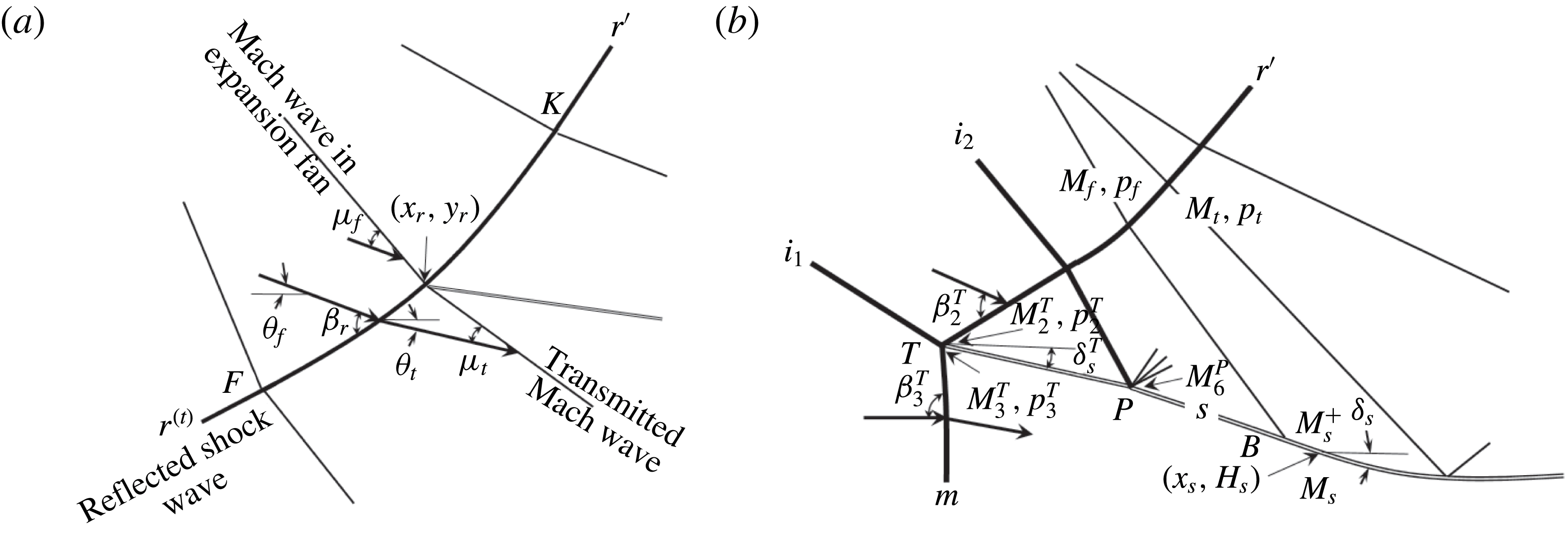
Figures 4 and 5 display the overall Mach reflection configuration used here for the Mach stem height. More details about the definition of flow parameters are given in figures 6 and 7.
Now we outline the major steps in determining the Mach stem height, see Bai & Wu (Reference Bai and Wu2017) for those details that are identical to single incident shock wave reflection.
Definition of flow parameters near the interacting part of the reflected shock wave (a) and near the slipline (b).

The Mach stem height
 $H_{T}$
is first guessed (for instance
 $H_{T}=(1/2)g$
) and then evaluated through an iterative process. In the following we will use the subscript
 $s$
to denote solutions for the slipline.
Step (a), triple point solution and shock interaction point solution. These solutions are independent of the Mach stem height and can be solved in advance. Once
 $M_{0}$
and
 $\unicode[STIX]{x1D703}_{w}$
are given, the triple point solution is given from the three-shock theory outlined in § 3.1.1. This three-shock theory gives the shock angles
 $\unicode[STIX]{x1D6FD}_{1_{a}}$
(first incident shock wave),
 $\unicode[STIX]{x1D6FD}_{2}^{T}$
(reflected shock wave) and
 $\unicode[STIX]{x1D6FD}_{3}^{T}$
(Mach stem), the Mach numbers
 $M_{1_{a}}$
,
 $M_{2}^{T}$
and
 $M_{3}^{T}$
, the pressures
 $p_{1_{a}}$
,
 $p_{2}^{T}$
and
 $p_{3}^{T}$
and the initial angle of the slipline
 $\unicode[STIX]{x1D6FF}_{s}^{T}$
. The superscript
 $T$
here means solutions near the triple point
 $T$
.
The shock/shock interaction theory outlined in § 3.1.2 gives solutions (Mach number
 $M_{j}$
, pressure
 $p_{j}$
, flow deviation angle
 $\unicode[STIX]{x1D703}_{j}$
) in regions
 $j=1_{b}$
, 4 and 5 and the shock angles
 $\unicode[STIX]{x1D6FD}_{1_{b}}$
,
 $\unicode[STIX]{x1D6FD}_{4}$
and
 $\unicode[STIX]{x1D6FD}_{5}$
.
Step (b), shock interaction point
 $O$
and shock/slipline reflection point
 $P$
. The positions of point
 $O$
and
 $P$
are dependent on the Mach stem height and are evaluated using the corresponding expressions in (3.19). The position
 $P$
will be further updated after the shape of the slipline segment
 $TP$
is computed.
Step (c), shape of the slipline before point
 $P$
. This is exactly the same as in Bai & Wu (Reference Bai and Wu2017). The inlet condition of the quasi-one-dimensional duct is defined as
 $M_{m}=(M_{3}^{T}+M_{G})/2$
and
 $p_{m}=(p_{3}^{T}+p_{G})/2$
, where
 $M_{G}$
and
 $p_{G}$
are normal shock solutions of the Mach number and pressure at the foot of the Mach stem.
The segment
 $TP$
of the slipline is a free part subjected to secondary Mach waves moving over it and, according to Bai & Wu (Reference Bai and Wu2017), its shape (height
 $H_{s}$
) is given by
 $$\begin{eqnarray}{\displaystyle \frac{H_{s}(x)}{H_{T}}}={\displaystyle \frac{M_{m}N^{-(\unicode[STIX]{x1D6FE}+1)/(2\unicode[STIX]{x1D6FE})}}{\sqrt{{\displaystyle \frac{2}{\unicode[STIX]{x1D6FE}-1}}(\unicode[STIX]{x1D717}(M_{m})N^{-(\unicode[STIX]{x1D6FE}-1)/\unicode[STIX]{x1D6FE}}\unicode[STIX]{x1D717}(M_{s}^{+})-1)}}}(\unicode[STIX]{x1D717}(M_{s}^{+}))^{(\unicode[STIX]{x1D6FE}+1)/(2\unicode[STIX]{x1D6FE}-2)},\end{eqnarray}$$
where
 $N=p_{2}^{T}/p_{3}(\unicode[STIX]{x1D717}(M_{2}^{T}))^{\unicode[STIX]{x1D6FE}/(\unicode[STIX]{x1D6FE}-1)}$
. The slipline deflection angle
 $\unicode[STIX]{x1D6FF}_{s}$
is related to
 $H_{s}$
by
 $$\begin{eqnarray}\unicode[STIX]{x1D6FF}_{s}(x)=-\text{arctan}\frac{\text{d}H_{s}}{\text{d}x}.\end{eqnarray}$$
Here,
 $M_{s}^{+}=M_{s}^{+}(x)$
is the Mach number just above the slipline and is related to the deflection angle of the slipline
 $\unicode[STIX]{x1D6FF}_{s}$
by the Prandtl–Meyer function
 $$\begin{eqnarray}\unicode[STIX]{x1D708}(M_{s}^{+})=\unicode[STIX]{x1D6FF}_{s}-\unicode[STIX]{x1D6FF}_{s}^{T}+\unicode[STIX]{x1D708}(M_{2}^{T}).\end{eqnarray}$$
See (3.2) for
 $\unicode[STIX]{x1D708}(M)$
and
 $\unicode[STIX]{x1D717}(M)$
. Expression (4.1) was obtained by pressure balance between the quasi-one-dimensional duct and secondary expansion waves over the slipline.
Step (d), shape of the slipline between
 $P$
and
 $B$
. Here, due to the reflection of the transmitted part
 $i_{2}^{(t)}$
of the second incident shock wave, the slipline changes angle at point
 $P$
to have an additional deflection angle
 $\unicode[STIX]{x1D6FF}_{P}$
as obtained in § 3.1.3, see expression (3.11).
Since the height of the slipline
 $H_{s}$
before point
 $P$
has been obtained more accurately in step (c), the position of point
 $P$
is now updated as
 $$\begin{eqnarray}\frac{y_{O}-y_{P}}{x_{O}-x_{P}}=\tan (\unicode[STIX]{x1D6FD}_{4}+\unicode[STIX]{x1D703}_{2}),\quad y_{P}=H_{s}(x_{P}),\end{eqnarray}$$
where the position
 $(x_{O},y_{O})$
is given in (3.19). See step (a) for
 $\unicode[STIX]{x1D6FD}_{4}$
and
 $\unicode[STIX]{x1D703}_{2}$
. The shape of slipline
 $PB$
is similarly defined as in step (c), starting now from point
 $P$
. The expressions (4.1)–(4.3) are still used here, but with
 $M_{m},M_{2}^{T}$
and
 $\unicode[STIX]{x1D6FF}_{s}^{T}$
replaced by
 $M_{s}(x_{P}),M_{6}^{P}$
and
 $\unicode[STIX]{x1D6FF}_{s}(x_{P})+\unicode[STIX]{x1D6FF}_{P}$
, respectively. Here
 $M_{6}^{P}$
is the Mach number in region
 $6$
but near point
 $P$
, given by (3.11),
 $M_{s}(x_{P})$
is the Mach number of the quasi-one-dimensional duct at point
 $x=x_{P}$
, given by
 $$\begin{eqnarray}\frac{H_{s}(x_{P})}{H_{T}}=\frac{M_{m}}{M_{s}(x_{P})}\left(\frac{\unicode[STIX]{x1D717}(M_{s}(x_{P}))}{\unicode[STIX]{x1D717}(M_{m})}\right)^{(\unicode[STIX]{x1D6FE}+1)/(2\unicode[STIX]{x1D6FE}-2)}.\end{eqnarray}$$
This step is continued to point
 $B$
where the slipline intersects the first characteristic of the transmitted Mach waves from the wedge corner expansion fan. After this point is the interacting part (
 $BE$
) of the slipline, which depends on the shape of the reflected shock wave.
Step (e), shape of the reflected shock wave
 $FK$
. The first characteristics of the wedge expansion fan intersects the transmitted reflected shock wave
 $r^{(t)}$
at point
 $F$
. The shock segment
 $OF$
is assumed to be straight, so that the position
 $(x_{F},y_{F})$
can be determined by (3.18), see (3.19) for the explicit expression.
The shape of the reflected shock wave follows from the analytical shock/expansion wave interaction algorithm given by Bai & Wu (Reference Bai and Wu2017), with minor modification for the upstream condition. Let
 $\unicode[STIX]{x1D703}_{f}$
be the deflection angle of the flow stream in the expansion fan, with
 $\unicode[STIX]{x1D703}_{f}=\unicode[STIX]{x1D703}_{W}+\unicode[STIX]{x1D6FF}$
for the leading characteristic
 $RF$
. When the flow direction deflects downwards,
 $\unicode[STIX]{x1D703}_{f}$
is considered positive. For any given
 $\unicode[STIX]{x1D703}_{f}$
, the Mach number
 $M_{f}$
and the pressure
 $p_{f}$
in the expansion fan follow from the Prandtl–Meyer solution. The interacting part (segment FK in figure 4) of the reflected shock wave has a shock angle
 $\unicode[STIX]{x1D6FD}_{r}$
following the expression according to Bai & Wu (Reference Bai and Wu2017)
 $$\begin{eqnarray}\frac{\text{d}\unicode[STIX]{x1D6FD}_{r}}{\text{d}\unicode[STIX]{x1D703}_{f}}=\frac{(\unicode[STIX]{x1D6FD}_{\unicode[STIX]{x1D703}}-K_{5}\unicode[STIX]{x1D6FD}_{M})-\unicode[STIX]{x1D6FD}_{\unicode[STIX]{x1D703}}K_{4}K_{3}}{1+2\unicode[STIX]{x1D6FD}_{\unicode[STIX]{x1D703}}K_{4}\sin (2\unicode[STIX]{x1D6FD}_{r})},\quad \unicode[STIX]{x1D6FD}_{r}=\unicode[STIX]{x1D6FD}_{5}\text{ at }\unicode[STIX]{x1D703}_{f}=\unicode[STIX]{x1D703}_{w}+\unicode[STIX]{x1D6FF}.\end{eqnarray}$$
The abscissa
 $x_{r}$
on the reflected shock is connected to
 $\unicode[STIX]{x1D703}_{f}$
through
 $$\begin{eqnarray}\frac{\text{d}x_{r}}{\text{d}\unicode[STIX]{x1D703}_{f}}=\frac{1-M_{f}^{2}-\unicode[STIX]{x1D717}(M_{f})}{M_{f}^{2}-1}\frac{\tan ^{2}(\unicode[STIX]{x1D703}_{f}+\unicode[STIX]{x1D707}_{f})+1}{\tan (\unicode[STIX]{x1D6FD}_{r}-\unicode[STIX]{x1D703}_{f})+\tan (\unicode[STIX]{x1D703}_{f}+\unicode[STIX]{x1D707}_{f})}(x_{r}-x_{R}),\end{eqnarray}$$
where
 $\unicode[STIX]{x1D707}_{f}$
is the Mach angle at
 $M_{f}$
. The parameters involved in (4.6) are defined by
 $$\begin{eqnarray}\left.\begin{array}{@{}c@{}}\unicode[STIX]{x1D6FD}_{\unicode[STIX]{x1D703}}=[1-K_{1}+2K_{2}M_{f}\cos ^{2}\unicode[STIX]{x1D6FD}_{r}]^{-1},\\ \unicode[STIX]{x1D6FD}_{M}=-[1-K_{1}+2K_{2}\cos ^{2}\unicode[STIX]{x1D6FD}_{r}]^{-1}K_{2}\sin (2\unicode[STIX]{x1D6FD}_{r}),\\ K_{1}={\displaystyle \frac{\sin 2(\unicode[STIX]{x1D6FD}_{r}-\unicode[STIX]{x1D703}_{f}+\unicode[STIX]{x1D703}_{t})}{\sin (2\unicode[STIX]{x1D6FD}_{r})}},\quad K_{2}={\displaystyle \frac{2(\unicode[STIX]{x1D6FE}+1)M_{f}\sin ^{2}(\unicode[STIX]{x1D6FD}_{r}-\unicode[STIX]{x1D703}_{f}+\unicode[STIX]{x1D703}_{t})}{[(\unicode[STIX]{x1D6FE}-1)M_{f}^{2}\sin ^{2}\unicode[STIX]{x1D6FD}_{r}+2]^{2}}},\\ K_{5}={\displaystyle \frac{M_{f}}{\sqrt{M_{f}^{2}-1}}}\unicode[STIX]{x1D717}(M_{f}),\\ \unicode[STIX]{x1D703}_{t}=\unicode[STIX]{x1D703}_{f}-\arctan \left(2\cot \unicode[STIX]{x1D6FD}_{r}{\displaystyle \frac{M_{f}^{2}\sin ^{2}\unicode[STIX]{x1D6FD}_{r}-1}{M_{f}^{2}(\unicode[STIX]{x1D6FE}+\cos 2\unicode[STIX]{x1D6FD}_{r})+2}}\right).\end{array}\right\}\end{eqnarray}$$
Starting from point
 $F$
, where the shock angle is
 $\unicode[STIX]{x1D6FD}_{r}=\unicode[STIX]{x1D6FD}_{5}$
, solve (4.6), (4.7) and
 $\text{d}y_{r}/\text{d}x_{r}=\tan (\unicode[STIX]{x1D6FD}_{r}-\unicode[STIX]{x1D703}_{f})$
to find
 $\unicode[STIX]{x1D6FD}_{r}=\unicode[STIX]{x1D6FD}_{r}(\unicode[STIX]{x1D703}_{f})$
and the position of the reflected shock wave
 $(x_{r},y_{r})$
for
 $\unicode[STIX]{x1D703}_{f}$
varying from
 $\unicode[STIX]{x1D703}_{w}+\unicode[STIX]{x1D6FF}$
to 0. At any
 $\unicode[STIX]{x1D703}_{f}$
or
 $(x_{r},y_{r})$
, the quantities
 $M_{t}$
and
 $p_{t}$
(solutions just downstream of the reflected shock wave) are connected to
 $M_{f}$
and
 $p_{f}$
through the oblique shock wave expressions, with the shock angle
 $\unicode[STIX]{x1D6FD}_{r}$
.
Step (f), shape of the interacting part of slipline (after point
 $B$
). The shape of the interacting part of the slipline depends on the transmitted expansion waves from the expansion fan since they bring information of the pressure waves from below the reflected shock waves to the slipline. Bai & Wu (Reference Bai and Wu2017) used straight characteristic line assumption for these transmitted expansion waves, although they are perturbed by the secondary waves from the free part
 $TB$
of the slipline. Here the problem is further complicated due to the second incident shock wave, which splits the flow regions into regions 4, 5 and 6 by shock interaction at point
 $O$
and shock reflection at point
 $P$
. Here, to capture the main physics we still use the straight characteristic line assumption and the flow upstream of the leading characteristics
 $FB$
is taken from solution of region 6. This assumption appears to hold in single incident shock wave case, according to the transmitted expansion waves displayed by Gao & Wu (Reference Gao and Wu2010), and is supposed to hold here for weak values of
 $\unicode[STIX]{x1D6FF}$
.
The position (
 $x_{B},y_{B}$
) of
 $B$
can be determined through
 $y_{B}=H_{s}(x_{B})$
and
 $y_{B}-y_{F}=-(x_{B}-x_{F})\tan (\unicode[STIX]{x1D707}_{F}+\unicode[STIX]{x1D703}_{6}^{P})$
where
 $\unicode[STIX]{x1D707}_{F}=\arcsin (1/M_{6}^{P})$
and
 $\unicode[STIX]{x1D703}_{6}^{P}=\unicode[STIX]{x1D6FF}_{s}^{P}$
. With point
 $B$
thus determined and with
 $M_{t}$
,
 $p_{t}$
determined through step (e), the expressions for the shape of the slipline after point
 $B$
are the same as those given by Bai & Wu (Reference Bai and Wu2017).
The deflection angle of the slipline
 $\unicode[STIX]{x1D6FF}_{s}$
satisfies
 $$\begin{eqnarray}\frac{\unicode[STIX]{x1D6FE}p_{t}M_{t}^{2}}{\sqrt{M_{t}^{2}-1}}\frac{\text{d}\unicode[STIX]{x1D6FF}_{s}}{\text{d}x_{s}}+\frac{\unicode[STIX]{x1D6FE}p_{f}M_{f}^{2}(K_{6}+K_{7})}{\unicode[STIX]{x1D6FE}+1}\unicode[STIX]{x1D6F9}(\unicode[STIX]{x1D6FF}_{s})^{-1}+\frac{\unicode[STIX]{x1D6FE}M_{s}^{2}}{1-M_{s}^{2}}\frac{p_{s}}{H_{s}}\tan \unicode[STIX]{x1D6FF}_{s}=0,\end{eqnarray}$$
where
 $$\begin{eqnarray}K_{6}=\frac{1-\unicode[STIX]{x1D6FE}-2\sin ^{2}\unicode[STIX]{x1D6FD}_{r}(2-M_{f}^{2})}{\sqrt{M_{f}^{2}-1}},\quad K_{7}=2\sin (2\unicode[STIX]{x1D6FD}_{r})\frac{(\unicode[STIX]{x1D6FD}_{\unicode[STIX]{x1D703}}-K_{5}\unicode[STIX]{x1D6FD}_{M})-\unicode[STIX]{x1D6FD}_{\unicode[STIX]{x1D703}}K_{4}K_{3}}{1+2\unicode[STIX]{x1D6FD}_{\unicode[STIX]{x1D703}}K_{4}\sin (2\unicode[STIX]{x1D6FD}_{r})}.\end{eqnarray}$$
The abscissa
 $x_{s}$
of the slipline is related to
 $\unicode[STIX]{x1D703}_{f}$
by
 $$\begin{eqnarray}\frac{\text{d}x_{s}}{\text{d}\unicode[STIX]{x1D703}_{f}}=\unicode[STIX]{x1D6F9}(\unicode[STIX]{x1D6FF}_{s}),\quad \unicode[STIX]{x1D6F9}(\unicode[STIX]{x1D6FF}_{s})=\frac{(K_{6}+K_{7})p_{f}M_{f}^{2}\sqrt{M_{t}^{2}-1}}{(\unicode[STIX]{x1D6FE}+1)p_{t}M_{t}^{2}}\unicode[STIX]{x1D6EC},\end{eqnarray}$$
where
 $$\begin{eqnarray}\unicode[STIX]{x1D6EC}=-\frac{\tan ^{2}(\unicode[STIX]{x1D707}_{t}+\unicode[STIX]{x1D703}_{t})+1}{(\tan (\unicode[STIX]{x1D707}_{t}+\unicode[STIX]{x1D703}_{t})-\tan \unicode[STIX]{x1D6FF}_{s})}\frac{M_{t}^{2}-1+\unicode[STIX]{x1D717}(M_{t})}{M_{t}^{2}-1}(x_{s}-x_{r})\end{eqnarray}$$
and
 $x_{r}=x_{r}(\unicode[STIX]{x1D703}_{f})$
is the abscissa at the reflected shock wave
 $FK$
. The flow parameters below the slipline are related to
 $H_{s}=H_{s}(x)$
through the quasi-one-dimensional isentropic flow relations.
Starting from point
 $B$
, and knowing
 $M_{t}$
and
 $p_{t}$
from step (e), the expressions (4.9) and (4.11) are used to find
 $x_{s}$
,
 $\unicode[STIX]{x1D6FF}_{s}=\unicode[STIX]{x1D6FF}_{s}(x_{s})$
and
 $H_{s}=H_{s}(x_{s})$
, for any
 $\unicode[STIX]{x1D703}_{f}$
varying from
 $\unicode[STIX]{x1D703}_{w}$
to 0.
 $H_{s}$
follows from
 $\unicode[STIX]{x1D6FF}_{s}$
through
 $\text{d}H_{s}/\text{d}x=\tan \unicode[STIX]{x1D6FF}_{s}$
.
Step (g), Mach stem height following the sonic throat compatibility condition. The initial guess of the Mach stem height
 $H_{T}$
is now updated to meet the sonic throat compatibility condition (Bai & Wu Reference Bai and Wu2017). Step (f) gives one throat position
 $x_{sonic}$
, with
 $\unicode[STIX]{x1D6FF}_{s}(x_{sonic})=0$
. Use the quasi-one-dimensional isentropic relation to find the Mach number
 $M_{s}$
in the quasi-one-dimensional duct. This gives another throat position
 $x_{M}$
, with
 $M_{s}(x_{M})=M_{s}^{\ast }=1$
.
If
 $x_{sonic}=x_{M}$
, then the initial choice of the Mach stem height is correct and is said to meet the sonic throat compatibility condition. If
 $x_{sonic}\neq x_{M}$
, then the choice of the Mach stem height
 $H_{T}$
is incorrect and should be updated until
 $x_{sonic}=x_{M}$
. The method of bisection given by Bai & Wu (Reference Bai and Wu2017) can then be used to update the Mach stem height. For given
 $M_{0}$
,
 $\unicode[STIX]{x1D703}_{w}$
,
 $\unicode[STIX]{x1D6FF}$
and
 $g\cos \unicode[STIX]{x1D703}_{w}/L$
, the height of the Mach stem thus determined is unique.
5 Theoretical and numerical study of the role of the second incident shock wave
In this section, we study the role of the second incident shock wave in the uniform flow properties near the interaction points, using the exact solutions presented in § 3 and CFD computations. The influence of the second incident shock wave on the Mach stem height is studied using CFD simulations and the approximate model presented in § 4. Though the Mach stem height model is intended only for small
 $\unicode[STIX]{x1D6FF}$
, here we also apply it to high
 $\unicode[STIX]{x1D6FF}$
.
5.1 Uniform flow solution and slipline deflection angle
$\unicode[STIX]{x1D6FF}_{P}$

Here, we show results only for two sets of conditions. One is
 $M_{0}=3.98$
and
 $\unicode[STIX]{x1D703}_{w}=23.5^{\circ }$
, the other is
 $M_{0}=5$
and
 $\unicode[STIX]{x1D703}_{w}=23.5^{\circ }$
. For each set, three values of
 $\unicode[STIX]{x1D6FF}$
are considered. The uniform flow solutions in regions 4 and 6 (in the vicinity of point
 $P$
, see figure 5
a and § 3.1 for method) and the slipline deflection angle
 $\unicode[STIX]{x1D6FF}_{T}$
(near the triple point) and
 $\unicode[STIX]{x1D6FF}_{P}$
(additional deflection angle of the slipline at point
 $P$
) are computed using the theoretical model (see § 3.1.1 for
 $\unicode[STIX]{x1D6FF}_{T}$
and § 3.1.3 for
 $\unicode[STIX]{x1D6FF}_{P}$
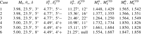
). They are also measured from CFD results. The results, with comparison between theory and CFD, are shown in table 1.
Mach contours showing that
 $P$
and
 $B$
are well separated for small
 $\unicode[STIX]{x1D6FF}$
and very close for large
 $\unicode[STIX]{x1D6FF}$
. (a)
 $M_{0}=5$
and
 $\unicode[STIX]{x1D703}_{w}=23.5^{\circ }$
,
 $\unicode[STIX]{x1D6FF}=5^{\circ }$
, (b)
 $M_{0}=5$
and
 $\unicode[STIX]{x1D703}_{w}=23.5^{\circ }$
,
 $\unicode[STIX]{x1D6FF}=8^{\circ }$
.

Comparison of flow parameters between theory and CFD. For
 $\unicode[STIX]{x1D6FF}_{T}$
measured from CFD, we use
 $+$
and
 $-$
to mean values slightly greater than or less than, since it is difficult to measure angles to within an accuracy of one degree.
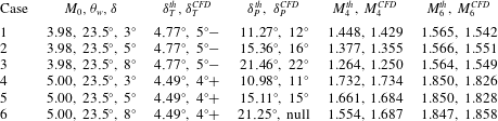
The theory compares well with the CFD results, although a discrepancy exists due to the simplification of the solution in region 2 (this solution is non-uniform due to Mach waves over the slipline, according to Gao & Wu (Reference Gao and Wu2010)) and due to measurement error of the slipline angle from the CFD results.
Both theory and CFD show that the additional deflection angle of the slipline
 $\unicode[STIX]{x1D6FF}_{P}$
is even greater than the additional wedge deflection angle
 $\unicode[STIX]{x1D6FF}$
. For the same
 $\unicode[STIX]{x1D6FF}$
and
 $\unicode[STIX]{x1D703}_{w}$
,
 $\unicode[STIX]{x1D6FF}_{P}$
decreases with increasing
 $M_{0}$
.
It is difficult to measure
 $\unicode[STIX]{x1D6FF}_{P}$
from the Mach contours for
 $M_{0}=5$
,
 $\unicode[STIX]{x1D703}_{w}=23.5^{\circ }$
and
 $\unicode[STIX]{x1D6FF}=8^{\circ }$
, since for this set of conditions, the point
 $P$
is too close to
 $B$
(
 $P$
is the shock/slipline interacting point and
 $B$
is the intersection of slipline and leading characteristics of the transmitted expansion waves, see figure 4). The fact that
 $P$
and
 $B$
are close, as displayed in figure 8, makes the segment
 $PB$
poorly resolved in CFD computation so that it is difficult to measure
 $\unicode[STIX]{x1D6FF}_{P}$
.
Both theory and CFD show that the additional deflection angle
 $\unicode[STIX]{x1D6FF}_{P}$
of the slipline is large and sensitive to
 $\unicode[STIX]{x1D6FF}$
. For instance, at
 $M_{0}=3.98$
and
 $\unicode[STIX]{x1D6FF}=8^{\circ }$
, the value of
 $\unicode[STIX]{x1D6FF}_{P}$
may exceed
 $20^{\circ }$
. This means that the flow duct below the slipline is highly convergent, which may greatly affect the Mach stem height, as discussed below.
In case that
 $\unicode[STIX]{x1D6FF}_{P}$
is large for large
 $\unicode[STIX]{x1D6FF}$
, the quasi-one-dimensional flow model for the duct between the slipline and reflecting surface may be not suitable. The Mach stem height model where the quasi-one-dimensional flow assumption is used may not work for large
 $\unicode[STIX]{x1D6FF}_{P}$
or
 $\unicode[STIX]{x1D6FF}$
, as shown below.
5.2 Dependence of Mach stem height on the strength of second incident shock wave
Here we put
 $g\cos \unicode[STIX]{x1D703}_{w}/L=0.4$
,
 $\unicode[STIX]{x1D703}_{w}=23.5^{\circ }$
and consider two Mach numbers,
 $M_{0}=3.98$
and
 $M_{0}=5$
.
Variation of the relative Mach stem height
 $H_{T}/L$
for various
 $\unicode[STIX]{x1D6FF}$
for
 $\unicode[STIX]{x1D703}_{w}=23.5^{\circ }$
,
 $g\cos \unicode[STIX]{x1D703}_{w}/L=0.4$
. (a)
 $M_{0}=3.98$
, (b)
 $M_{0}=5$
.

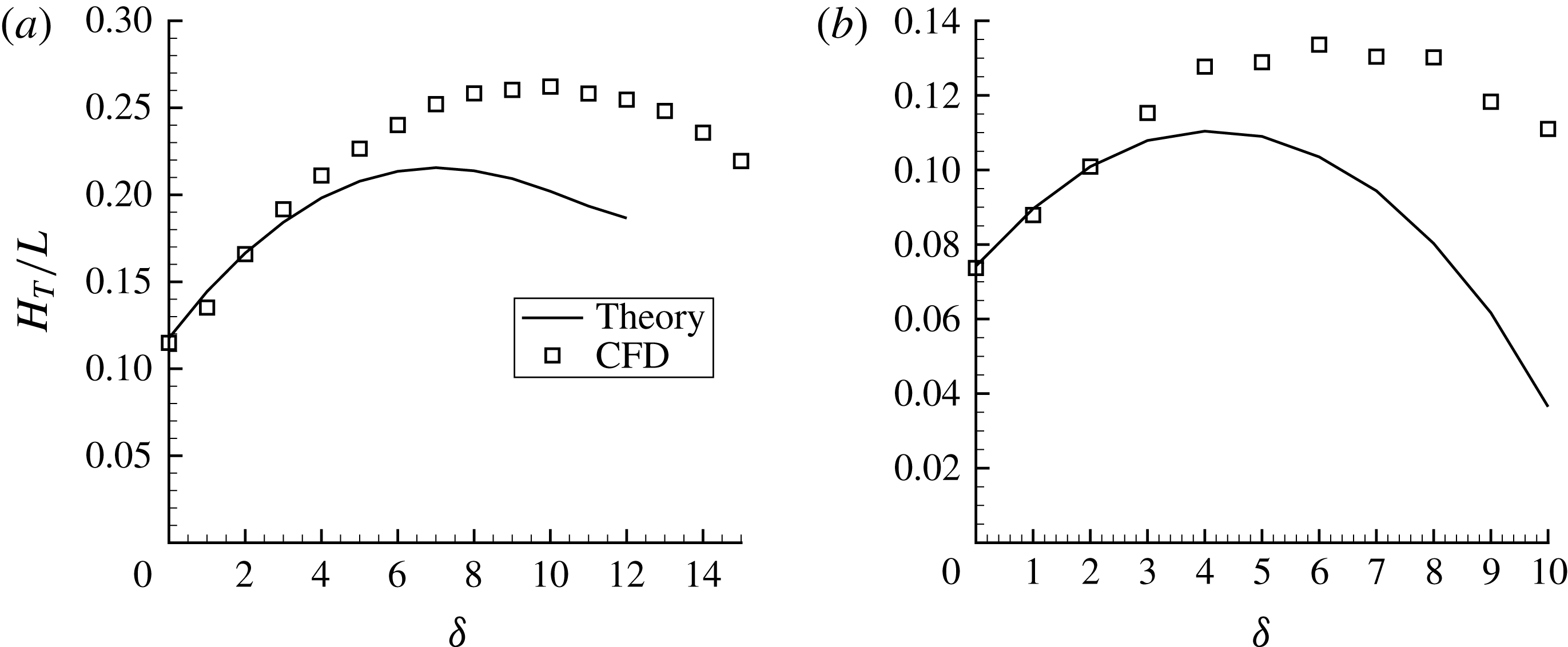
The relative Mach stem heights
 $H_{T}/L$
for a series of additional wedge deflection angles
 $\unicode[STIX]{x1D6FF}$
are displayed in figure 9(a) for
 $M_{0}=3.98$
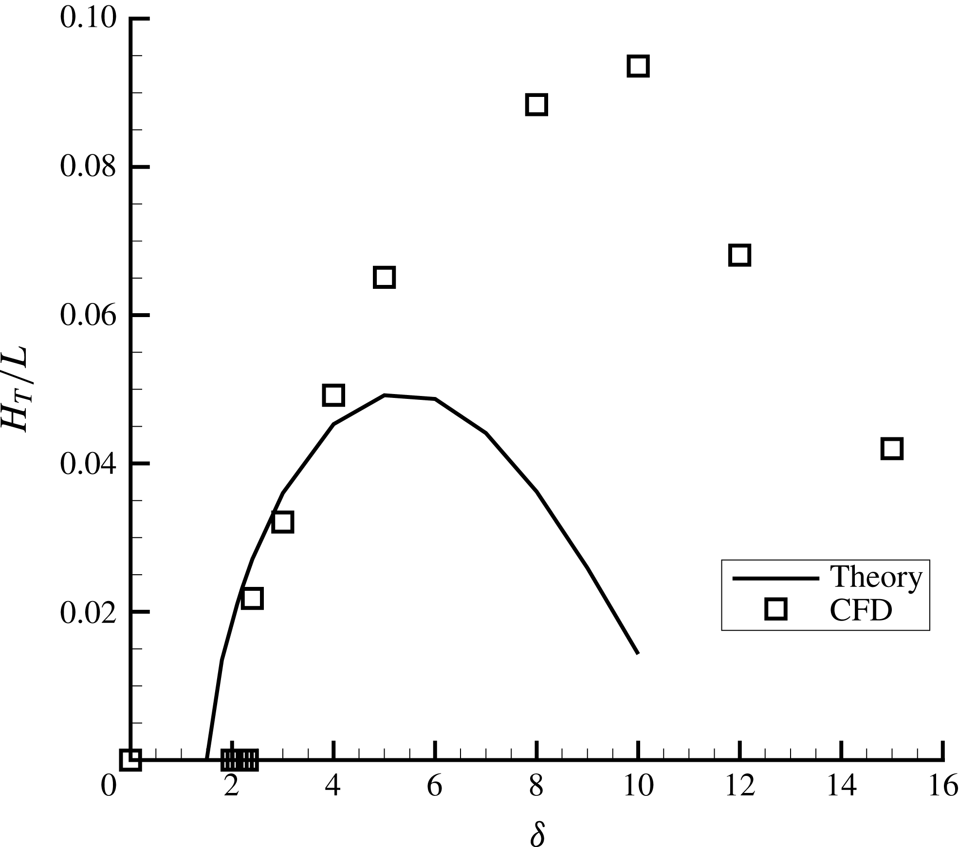
and in figure 9(b) for
 $M_{0}=5$
. The results of both theory and CFD are shown.
The theory agrees well with CFD when
 $\unicode[STIX]{x1D6FF}=0^{\circ }$
(which corresponds to Mach reflection with a single incident shock wave). This is not surprise since in this case the theory reduces to the model by Bai & Wu (Reference Bai and Wu2017) and this model has been checked out for accuracy. The good comparison also shows that the grid used for CFD is suitable for the single incident shock wave case.
Moreover, when
 $\unicode[STIX]{x1D6FF}>0^{\circ }$
but remains small enough (
 $\unicode[STIX]{x1D6FF}\leqslant 2^{\circ }$
), the theory also compares well with CFD. Hence, the theory can be used to explain the influence of the second incident shock wave for small
 $\unicode[STIX]{x1D6FF}$
.
However, for
 $\unicode[STIX]{x1D6FF}$
large enough (exceeding for instance
 $3^{\circ }$
), the discrepancy is large, for reasons to be discussed in § 6.1. Despite the discrepancy for large
 $\unicode[STIX]{x1D6FF}$
, we may draw two interesting conclusions:
(i) the Mach stem height is increased by the second incident shock wave;
(ii) the Mach stem height does not increase monotonically with
$\unicode[STIX]{x1D6FF}$
(which characterizes the strength of the second incident shock wave) and there is a maximum of the Mach stem height at some
$\unicode[STIX]{x1D6FF}$
. It is interesting that, although the theoretical model does not apply to high
$\unicode[STIX]{x1D6FF}$
, it successfully predicts a maximum.


Below we discuss the underlying mechanisms related to these phenomena.
5.3 Discussion of the underlying mechanisms for the observed phenomena
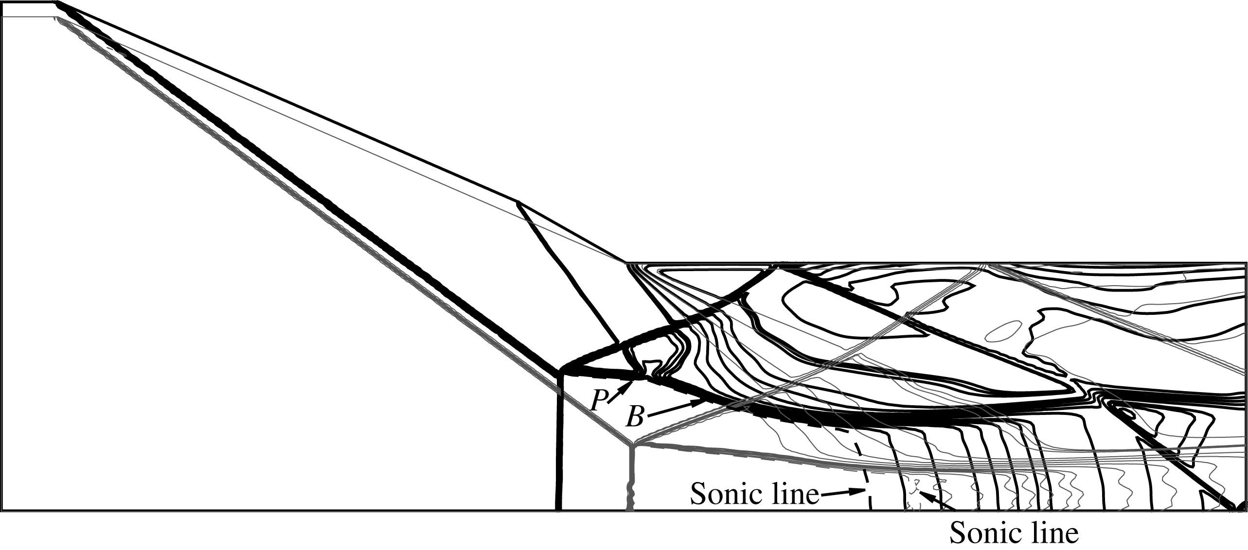
We first explain why the Mach stem height is increased by the existence of the second incident shock wave. For this purpose, we superimpose, for
 $M_{0}=3.98$
,
 $\unicode[STIX]{x1D703}_{w}=23.5^{\circ }$
, the Mach contours with
 $\unicode[STIX]{x1D6FF}=0^{\circ }$
(single incident shock wave) and
 $\unicode[STIX]{x1D6FF}=6^{\circ }$
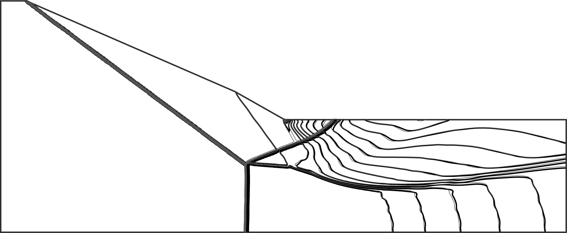
(double incident shock waves) in figure 10. It is seen that before point B (the intersection of the slipline and the leading characteristics of the transmitted Mach waves of the expansion fan from the trailing edge), the quasi-one-dimensional flow duct below the slipline converges more rapidly when
 $\unicode[STIX]{x1D6FF}$
increases from
 $0^{\circ }$
to
 $6^{\circ }$
.
Mach contours of Mach reflection for single and double incident shock waves,
 $M_{0}=3.98$
,
 $\unicode[STIX]{x1D703}_{w}=23.5^{\circ }$
,
 $g\cos \unicode[STIX]{x1D703}_{w}/L=0.4$
. Dark lines: double incident shock waves with
 $\unicode[STIX]{x1D6FF}=6^{\circ }$
, grey lines: single incident shock wave with
 $\unicode[STIX]{x1D6FF}=0^{\circ }$
.

In the case of single incident shock wave, Tan, Ren & Wu (Reference Tan, Ren and Wu2006) displayed in the plane
 $(M_{0},\unicode[STIX]{x1D703}_{w})$
the slipline angle
 $\unicode[STIX]{x1D6FF}_{T}$
(see their figure 4) while Gao & Wu (Reference Gao and Wu2010) displayed in the plane
 $(M_{0},\unicode[STIX]{x1D703}_{w})$
the relative Mach stem height for
 $w/H_{A}=1.1$
(see their figure 16). Comparing these two figures, it is seen that the Mach stem height increases when the slipline angle increases. The reason to have this dependence can be explained as follows. The size of the Mach stem is determined by the sonic throat compatibility condition (Bai & Wu Reference Bai and Wu2017). This sonic throat is established due to the pressure dropping effect by the transmitted expansion Mach waves from the wedge corner expansion fan.
There are two interacting mechanisms to drive the sonic throat compatibility condition to be satisfied. The convergence of the quasi-one-dimensional duct will drive the Mach number in this duct to reach 1 (sonic point). The pressure dropping effect by the impingement and reflection of the transmitted expansion waves over the slipline makes the slipline shift in the horizontal direction to have a throat (i.e. the local slipline deflection angle
 $\unicode[STIX]{x1D6FF}_{s}=0$
).
If the Mach stem height is too small, the convergence effect of the quasi-one-dimensional duct dominates so that the sonic condition reaches at a point before the throat point. If the Mach stem height is too large, the pressure dropping effect by the transmitted expansion waves dominates so that the throat reaches at a point before the sonic point. The sonic point must coincide with the throat position so that the Mach stem height is unique.
Obviously, in the case of double incident shock wave studied here, the reflection of the second incident shock wave over the slipline at point
 $P$
makes the quasi-one-dimensional duct converge at a greater rate than without the second incident shock wave, so that sonic condition is reached earlier. To meet the sonic throat compatibility condition (or pressure balance across the slipline), the Mach stem and the slipline must be elevated to receive the fast pressure decreasing effect of the higher position of the transmitted expansion waves (the higher the position, the faster the pressure drops because of the quasi-fan sharper nature of the transmitted expansion waves).
Now we explain why there is a maximum of
 $H_{T}$
for some
 $\unicode[STIX]{x1D6FF}$
. To be more precise, for fixed
 $M_{0}$
and
 $\unicode[STIX]{x1D703}_{w}$
, the relative Mach stem height does not increase with
 $\unicode[STIX]{x1D6FF}$
monotonically. Both theory and CFD predict a maximum. A maximum of the (relative) Mach stem height is reached at some
 $\unicode[STIX]{x1D6FF}=\unicode[STIX]{x1D6FF}_{m}$
.
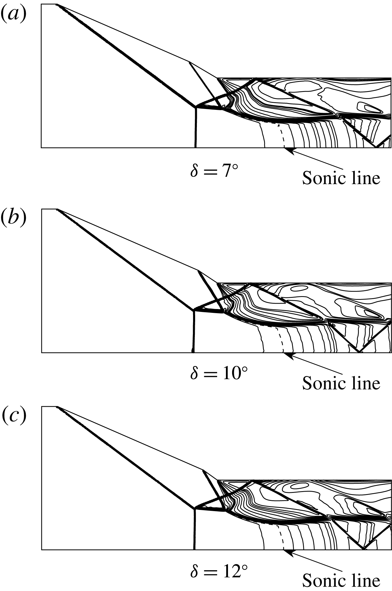
Mach contours of Mach reflection for double incident shock waves with three different
 $\unicode[STIX]{x1D6FF}$
. The other flow conditions are
 $M_{0}=3.98$
,
 $\unicode[STIX]{x1D703}_{w}=23.5^{\circ }$
, and
 $g\cos \unicode[STIX]{x1D703}_{w}/L=0.4$
.

For
 $M_{0}=3.98$
,
 $\unicode[STIX]{x1D703}_{w}=23.5^{\circ }$
, we have
 $\unicode[STIX]{x1D6FF}_{m}\approx 10^{\circ }$
from CFD data and
 $\unicode[STIX]{x1D6FF}_{m}\approx 7^{\circ }$
from theory. For
 $M_{0}=5$
,
 $\unicode[STIX]{x1D703}_{w}=23.5^{\circ }$
,
 $\unicode[STIX]{x1D6FF}_{m}\approx 7^{\circ }$
from CFD and
 $\unicode[STIX]{x1D6FF}_{m}\approx 4^{\circ }$
by theory. Note that there are some oscillations of the numerical Mach stem height near
 $\unicode[STIX]{x1D6FF}_{m}$
for the second case. This may be due to the fact that the Mach stem height is highly sensitive to the second incident shock wave near
 $\unicode[STIX]{x1D6FF}_{m}$
so that a slight inefficiency in resolving small structures such as Kelvin–Helmholtz unstable waves and secondary Mach waves would lead to such oscillation.
To see the reason for the existence of a maximum, we display in figure 11 the Mach contours for
 $M_{0}=3.98$
and
 $\unicode[STIX]{x1D703}_{w}=23.5^{\circ }$
, with
 $\unicode[STIX]{x1D6FF}=7^{\circ }<\unicode[STIX]{x1D6FF}_{m}$
,
 $\unicode[STIX]{x1D6FF}=10^{\circ }\approx \unicode[STIX]{x1D6FF}_{m}$
and
 $\unicode[STIX]{x1D6FF}=12^{\circ }>\unicode[STIX]{x1D6FF}_{m}$
.
It is clear that when
 $\unicode[STIX]{x1D6FF}$
is large enough, the reflection point
 $P$
is very close to the leading characteristics of the transmitted expansion waves. Above we have argued that the increase of Mach stem height by the second incident shock wave is due to the high convergence rate of the quasi-one-dimensional duct after point
 $P$
. However, when
 $\unicode[STIX]{x1D6FF}$
is very high, this duct with increased convergence rate spans only a short distance, before the leading characteristic of the transmitted expansion waves intersects the slipline. For instance, at the extreme case when
 $P$
touches this leading characteristic, the deflection
 $\unicode[STIX]{x1D6FF}_{p}$
at point
 $P$
has no role.
This explains the existence of a maximum of the Mach stem height at some
 $\unicode[STIX]{x1D6FF}$
.
6 Further considerations
In this section, we check the grid convergence of the numerical results and the flow field in the convergent duct to show the reason why the theory does not apply quantitatively for large
 $\unicode[STIX]{x1D6FF}$
. We also briefly study the influence of the nature of the top boundary downstream of the trailing edge, advance of regular to Mach reflection and the possible influence of viscosity.
6.1 Discussion of accuracy of CFD simulation and theory
As discussed in § 5.2, the discrepancy in the Mach stem heights between theory and CFD is large for large
 $\unicode[STIX]{x1D6FF}$
. In the case of large
 $\unicode[STIX]{x1D6FF}$
, the interaction points
 $P$
,
 $O$
and
 $B$
, as shown in figures 4 and 5, are confined in a narrow region. This means that the flow is highly complex and has a high gradient there. We thus wonder if the discrepancy between theory and CFD in predicting the Mach stem height at large
 $\unicode[STIX]{x1D6FF}$
partially comes from bad resolution of the CFD method. Here, we thus perform some calculations using a very refined grid.
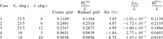
The number of cells used in §§ 2 and 5 is
 $180\times 460$
. Now we consider a very refined grid, with approximately
 $900\times 2300$
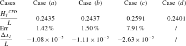
cells. Table 2 displays the Mach stem heights for several conditions.
Mach stem heights predicted by CFD using a coarse grid and a refined grid, compared to theory.
 $M_{0}=3.98$
.
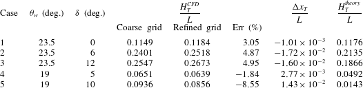
We see that the Mach stem heights predicted by the original coarse grid and the refined grid are very close, with a relative error (difference of Mach stem heights obtained by the refined grid and the coarse grid and divided by the coarse grid one) below 9 %. For the first three cases (
 $\unicode[STIX]{x1D703}_{w}=23.5^{\circ }$
), the refined grid gives a Mach stem height higher than the coarse grid, and the position of the Mach stem appears more upstream, as shown in table 2 (where
 $\unicode[STIX]{x0394}x_{T}$
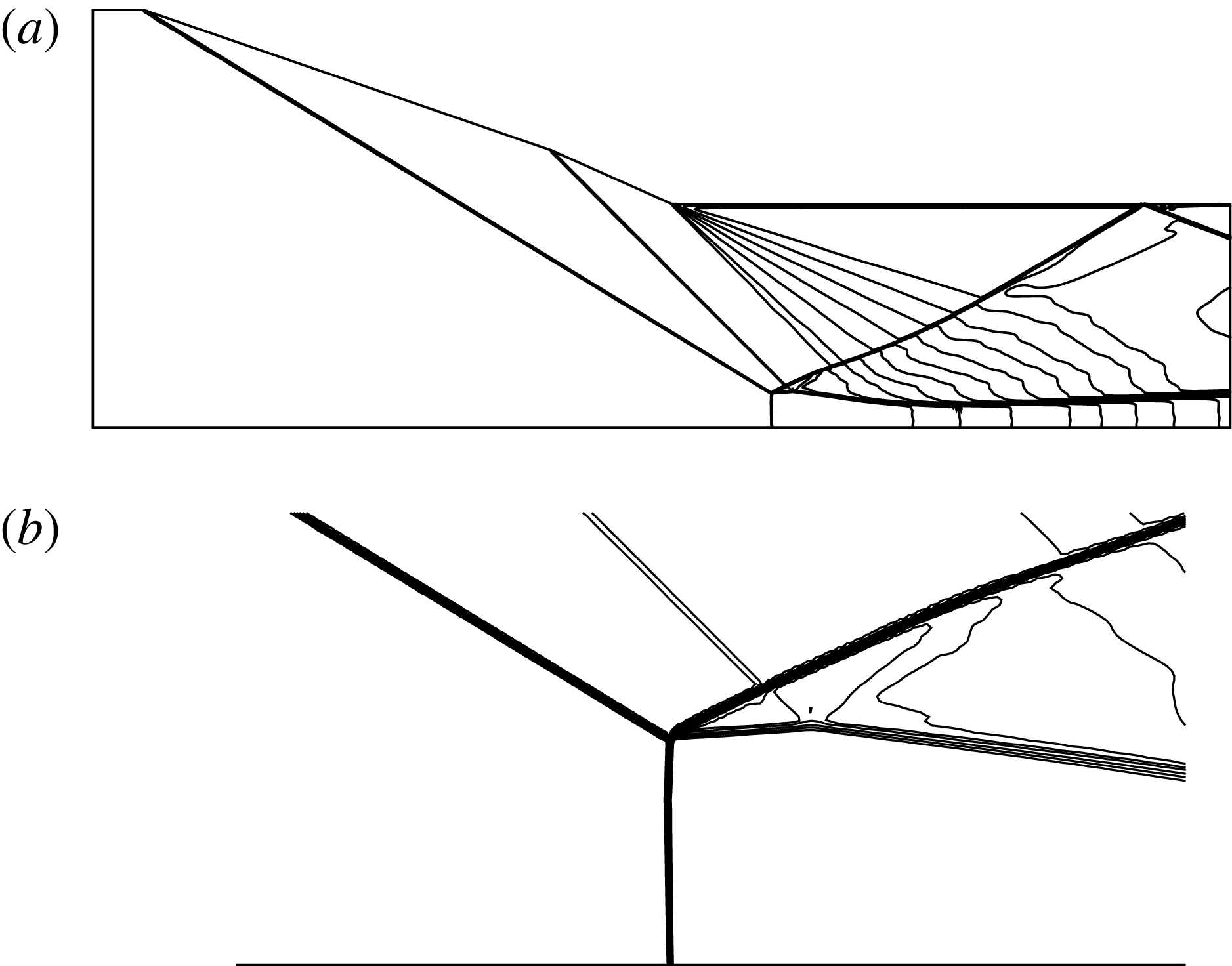
is the difference in the triple points of the refined grid and the coarse grid) since the triple point is along the first incident shock wave, so that the higher the Mach stem the more upstream it is. For the last two cases, the Mach stem height obtained by the refined grid is smaller than that obtained by coarse grid and the position of the Mach stem appears more downstream in the refined case. This discrepancy is significantly smaller than the discrepancy between theory and CFD, meaning that the discrepancy between theory and CFD is not due to the inaccuracy of the CFD calculations. However, the flow structures are more sharply resolved when the refined grid is used, as shown in figure 12 for
 $M_{0}=3.98$
,
 $\unicode[STIX]{x1D703}_{w}=23.5^{\circ }$
,
 $\unicode[STIX]{x1D6FF}=6^{\circ }$
.
Mach contours for
 $\unicode[STIX]{x1D6FF}=6^{\circ }$
,
 $\unicode[STIX]{x1D703}_{w}=23.5^{\circ }$
,
 $M_{0}=3.98$
. (a) Coarse grid, (b) fine grid.

Thus, the discrepancy is mainly due to a deficiency of the theoretical model for large
 $\unicode[STIX]{x1D6FF}$
. One reason may be that the flow duct below the slipline is highly convergent after the interaction point
 $P$
, so that quasi-one-dimensional flow model is not suitable.
Figure 13 displays the pressure contours inside the convergent duct for
 $\unicode[STIX]{x1D6FF}=0^{\circ }$
and
 $\unicode[STIX]{x1D6FF}=12^{\circ }$
, at
 $\unicode[STIX]{x1D703}_{w}=23.5^{\circ }$
,
 $M_{0}=3.98$
. It is clear that for
 $\unicode[STIX]{x1D6FF}=0^{\circ }$
the contour lines are almost vertical inside the convergent part of the duct below the slipline, meaning that the flow in the duct is almost one-dimensional and the quasi-one-dimensional flow model is usable. However, for
 $\unicode[STIX]{x1D6FF}=12^{\circ }$
the contour lines are non-vertical inside the convergent part of the duct below the slipline, meaning that the flow in the duct is essentially two-dimensional and the quasi-one-dimensional flow model is not usable.
This may explain that the theoretical model, which uses quasi-one-dimensional model for flow below the slipline, cannot give a quantitative prediction for a high value of
 $\unicode[STIX]{x1D6FF}$
. Thus, for high
 $\unicode[STIX]{x1D6FF}$
, one should rely on CFD or build a more advanced model.
Mach contours near the convergent duct
 $\unicode[STIX]{x1D703}_{w}=23.5^{\circ }$
,
 $M_{0}=3.98$
. (a)
 $\unicode[STIX]{x1D6FF}=0^{\circ }$
, (b)
 $\unicode[STIX]{x1D6FF}=12^{\circ }$
.

6.2 Influence of the top boundary downstream of the trailing edge
The influence of the type of the top boundary downstream of the trailing edge has never been considered before. Here we consider a comparison between results obtained using a solid wall condition and a non-reflecting boundary condition. Four cases are considered, the first two cases have this boundary at the same height of the inlet (similarly as the set-up of Ben-Dor et al. Reference Ben-Dor, Elperin, Li and Vasiliev1999) and the last two cases have this boundary at the same level of the rear wedge corner.
Figure 14 displays the Mach contours for comparison. It is seen that for the last treatment (where the top boundary is a wall), the flow field is contaminated with the reflected shock from the top wall (interacting with the subsonic–supersonic nozzle associated with the Mach stem).
Table 3 shows a comparison of the Mach stem heights. It is seen that, comparing with the solution of case (d) (this boundary type has been used in this paper), the Mach stem heights of the first two cases are slightly higher, also, the positions of the triple point of the first two cases are slightly further upstream. The Mach stem height of case (c) is higher than that of case (d), and the position of the triple point is further upstream.
Mach stem heights with different choices of top boundary condition downstream of the trailing edge, for
 $M_{0}=3.98$
,
 $\unicode[STIX]{x1D703}_{w}=23.5^{\circ }$
and
 $\unicode[STIX]{x1D6FF}=6^{\circ }$
. For cases (a) and (b), the top boundary is at the same height as the inlet (for case (a), the left boundary of the increased region is a non-reflecting one and for case (b) this boundary is a solid wall). For cases (c) and (d), the top boundary is at the same height as the rear edge of the wedge (for case (c), the top boundary is a non-reflecting one and for case (d), the boundary is a solid wall).

Mach stem heights with different treatments of the top boundary, the differences are relative to the case (d) solution. For the definitions of cases (a)–(d), see the caption of figure 14.
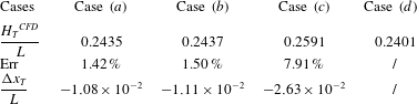
Thus, the Mach stem height is affected by the top boundary. This observation makes general sense even for Mach reflection with a single incident shock wave. In applications, the top boundary may be either a wall or an open boundary. Since the Mach stem heights for various choices of top boundary are different, a further study is required for this subject, to explain the reason for such a difference and to quantify the difference, even for a single incident shock wave reflection.
6.3 A preliminary study of the advance of regular to Mach transition and inverse-Mach stem
Ben-Dor et al. (Reference Ben-Dor, Elperin, Li and Vasiliev1999) observed, for their Mach reflection problem with a downstream pressure perturbation, an advance of the transition from RR to MR and an inverse-Mach reflection below the usual von Neumann criterion. This phenomenon occurs for the present double incident shock wave case, as shown in figure 3(b).
For
 $M_{0}=3.98$
, the von Neumann condition (in the case of single incident shock wave) corresponds to
 $\unicode[STIX]{x1D703}_{w}^{(N)}\approx 21^{\circ }$
. Now we display the results for
 $\unicode[STIX]{x1D703}_{w}=19^{\circ }$
, with various
 $\unicode[STIX]{x1D6FF}$
. As discussed in § 2.2, if both RR and MR are allowed, we adjust the computation to have a Mach reflection solution. Figure 15 displays the Mach contours with
 $\unicode[STIX]{x1D6FF}=5^{\circ }$
, using the refined grid. Although
 $\unicode[STIX]{x1D703}_{w}=19^{\circ }$
is below the usual von Neumann condition
 $\unicode[STIX]{x1D703}_{w}^{(N)}\approx 21^{\circ }$
, we observe Mach reflection, which is an inverse-Mach reflection. For inverse-Mach reflection, the Mach stem is convex toward the upstream direction and the initial angle of the slipline is negative (Henderson & Lozzi Reference Henderson and Lozzi1979; Hornung Reference Hornung1986; Hekiri & Emanuel Reference Hekiri and Emanuel2015).
Mach contours of inverse-Mach reflection, for
 $M_{0}=3.98$
,
 $\unicode[STIX]{x1D703}_{w}=19^{\circ }$
,
 $g\cos \unicode[STIX]{x1D703}_{w}/L=0.4$
,
 $\unicode[STIX]{x1D6FF}=5^{\circ }$
. (a) Overall view, (b) local view.

In figure 16, we display the Mach stem height for various
 $\unicode[STIX]{x1D6FF}$
. Mach reflection occurs when
 $\unicode[STIX]{x1D6FF}>2.4^{\circ }$
for the present case. Let us use ‘blunt body similarity’ to explain why the second incident shock wave may trigger the advance of transition for sufficiently large
 $\unicode[STIX]{x1D6FF}$
.
Roye, Henderson & Menikoff (Reference Roye, Henderson and Menikoff1998) provided a configuration (see their figure 6b) where an additional blunt body is placed along the reflecting surface and an inverted Mach reflection ahead of this blunt body is observed. This blunt body triggers a bow shock wave which is of course convex toward the upstream direction. The intersection of this bow shock with the incident shock wave produces a Mach stem. This means that the Mach stem is also a part of a bow shock, which is convex toward the upstream direction and thus inverted.
For the present problem, the second incident shock wave makes the slipline segment
 $PB$
deflect toward the reflecting surface. Such a declined segment plays a role equivalent to that of a blunt body, and is thus capable of inducing a bow shock and inverted Mach stem for similar reason as discussed above.
Inverted shock only occurs when the flow condition is in the domain below the usual von Neumann condition (Hekiri & Emanuel Reference Hekiri and Emanuel2015). This explains why the second incident shock wave can advance the transition.
For a given set of
 $M_{0}$
and
 $\unicode[STIX]{x1D703}_{w}$
in the RR domain, there should exist a value
 $\unicode[STIX]{x1D6FF}$
beyond which inverted Mach reflection occurs. A further study is required to obtain the theoretical value of this
 $\unicode[STIX]{x1D6FF}$
.
Variation of the relative Mach stem height
 $H_{T}/L$
for various
 $\unicode[STIX]{x1D6FF}$
. The input conditions are
 $M_{0}=3.98$
,
 $\unicode[STIX]{x1D703}_{w}=19^{\circ }$
and
 $g\cos \unicode[STIX]{x1D703}_{w}/L=0.4$
.

6.4 A preliminary consideration of the effect of viscosity
As in many previous studies with a single incident shock wave, here we have only considered inviscid flow. The influence of viscosity should be studied further because of the following two reasons.
(i) Viscosity is expected to increase the Mach stem height due to the increased displacement effect of the wedge boundary layer on Mach reflection.
(ii) The thickening of the shear layer emanating from the triple point by viscosity may also have some influence since the pressure across the shear layer balances over a finite distance.
These influences have been studied for single incident shock wave by Schmisseur & Gaitonde (Reference Schmisseur and Gaitonde2011) through CFD. They concluded that the Mach stem height is only modestly affected by viscosity when the Mach stem height is measured against the incident shock angle.
The displacement effect of the wedge boundary layer increases the equivalent wedge angle and thus the incident shock angle. For single incident shock wave reflection, a theoretical model has been proposed and will be published elsewhere. The displacement effect for the double incident shock wave case needs be studied in the future.
Schmisseur & Gaitonde (Reference Schmisseur and Gaitonde2011) also showed that no significant differences between inviscid and viscous calculations exist in the shear layers emanating from the triple point. To see whether this remark holds true in the double incident shock wave case, we perform a viscous computation (by solving the Navier–Stokes equations of compressible flow in which both the effects of viscosity and thermal conductivity are accounted for). For this purpose, we choose the case
 $M_{0}=3.98$
,
 $\unicode[STIX]{x1D703}_{w}=23.5^{\circ }$
and
 $\unicode[STIX]{x1D6FF}=6^{\circ }$
. The Reynolds number based on the inlet height
 $H_{A}$
is
 $8.5\times 10^{6}$
(this Reynolds number was used by Hornung & Robinson (Reference Hornung and Robinson1982) in their experimental study). Numerically, the inviscid part of the Navier–Stokes equations is solved using the same approach as for the inviscid flow, while the viscous and thermal conductive terms of the Navier–Stokes equations are approximated using second-order central differences. To isolate the influence of viscosity on shear layer, the wedge boundary layer is not resolved in this computation (since a detailed study of the influence of this boundary layer will be considered elsewhere).
Figure 17 displays a comparison of the Mach contours between inviscid and viscous flow computations. As in the study of Schmisseur & Gaitonde (Reference Schmisseur and Gaitonde2011), we observe no significant differences between inviscid and viscous calculations in the shear layers downstream of the triple points. The Mach stem height is slightly increased by viscosity, a conclusion already pointed out by Schmisseur & Gaitonde (Reference Schmisseur and Gaitonde2011). In the present case, the inviscid calculation gives
 $H_{T}/L=0.2591$
while the viscous calculation gives
 $H_{T}/L=0.2640$
, which is 1.89 % larger.
The present observation for viscous flow has been obtained only for a particular set of flow conditions. When the Reynolds number is much smaller, the thickening of the shear layer will be more pronounced so that the Mach stem height may be significantly affected. A theoretical model accounting for the thickening of the shear layer for shock reflection with small Reynolds number may be thus a subject for further study.
Mach contours for inviscid and viscous flows using non-reflecting condition on top boundary, with
 $\unicode[STIX]{x1D703}_{w}=23.5^{\circ }$
,
 $M_{0}=3.98$
,
 $\unicode[STIX]{x1D6FF}=6^{\circ }$
. Dark lines: inviscid flow, grey lines: viscous flow.

7 Concluding remarks
Mach reflection in steady supersonic flow with two incident shock waves is studied here. Using CFD it is shown that the second incident shock wave produces an additional shock/shock interaction point and a shock/slipline reflection point. Theoretical models are built for calculating flow parameters of the uniform flow regions and the positions of the interacting points. A Mach stem height model is updated from that of Bai & Wu (Reference Bai and Wu2017) for a single incident shock wave reflection to study the influence of the second incident shock wave. This model is valid for very small second deflection angles (
 $\unicode[STIX]{x1D6FF}\leqslant 2^{\circ }$
), i.e. it compares well with CFD results for
 $\unicode[STIX]{x1D6FF}\leqslant 2^{\circ }$
. For large second deflection angles, the model is qualitatively correct so that quantitative prediction should rely on CFD prediction or a more advanced model.
The shock/slipline reflection deflects the slipline towards the reflecting surface, elevating therefore the Mach stem height. Under the geometrical configuration we use in this paper, for a strong second incident shock wave, the variation of the Mach stem height as a function of the wedge deflection angle causing the second incident shock wave is non-monotonic. This is because when the incident shock wave is too strong, the slipline additional deflection (by the second incident shock wave), having the effect of elevating the Mach stem height, occurs over a reduced length of the slipline. Even though the flow condition is such that the first incident shock wave is below the usual von Neumann criterion, Mach reflection, i.e. inverted-Mach reflection, may be triggered by the second incident shock wave.
Three issues may form subjects of further study. The first is the critical condition for advanced RR to MR by the second incident shock wave. The second is to remove the geometric restriction that the two incident shock waves meet at the reflecting surface in the case of normal reflection. The third is related to viscous effects associated with the wedge boundary layer and thickenings of the shear layer, especially when the Reynolds number is small.
Acknowledgements
The referees provided valuable comments on this manuscript, which helped us to greatly improve the manuscript. This work was supported by the Natural National Science Foundation of China (no. 11802157).