THE UNITED STATES COMMISSION OF LABOR DATA

Because of its value as a trans-national survey, the data collected for the 1890 and 1891 Sixth and Seventh Reports of the USCL have been widely used in research, see for example, Michael R. Haines (Reference Haines1979), Timothy J. Hatton, George R. Boyer, and Roy E. Bailey (Reference Hatton, Boyer and Bailey1994), Sara Horrell and Deborah Oxley (Reference Horrell and Oxley1999), and Lynn Hollen Lees (Reference Lees and Merriman1979). The survey was conducted by Carroll D. Wright (1840–1909). It is known from Jeffery G. Williamson's (Reference Williamson1967) biographic sketch of Wright that he served in the Massachusetts Senate from 1871–1873, was persuaded to take over the Massachusetts Bureau of Statistics of Labor in 1873, and became the United States Commissioner for Labor in 1885. According to Williamson, Wright believed that “voluntary circulars were an inadequate source of data.” As a result, he developed and perfected advanced census techniques with face-to-face interviews in a number of enquiries in Massachusetts before the Sixth Annual Report in 1890 (Williamson Reference Williamson1967, pp. 102–3). According to Haines (Reference Haines1979, p. 272), Wright was “one of the United States’ great empirical statisticians.” Because the Sixth and Seventh Reports were motivated by the McKinley Tariff question, he was interested in estimating the cost of production and the standard of living in nine industries producing internationally traded goods (Williamson Reference Williamson1967, p. 105). Data were collected from 24 states in the United States and five European countries (Belgium, France, Germany, Great Britain, and Switzerland). Nearly one-third of the international sample related to cotton textiles (31.8), while less than 10 percent related to steel coke and iron ore (9.9 percent). Further, 97.8 percent of the households in the sample were male-headed households (Haines Reference Haines1979, pp. 293–4). For Britain, the sample comprised 1,024 households. The cotton, iron and steel, and Coal and coke industries were the most heavily represented. Most households, 777, declared themselves as English, with 128 Scottish, 80 Welsh, 38 Irish, and one declaring as Italian. There is only one female-headed household in the British sample.

The published reports provide only the briefest of description of the way in which families were selected and family structure and expenditure information recorded. The Report merely states (in relation to pig iron workers):

The Report highlights the fact that the families were asked to keep “accounts for a year's living” and that the word family is actually used to describe what we now define as households, as the family is defined as a “totality – husband, wife, children, boarders, everybody that goes to make up the household.”Footnote ⁴

It was not clear whether the sample was ever intended to be a random sample of families from the industries chosen. According to Lees (Reference Lees and Merriman1979, p. 170), the head of the travelling commissioners claimed that employers supplied wage data and that “home visits were made in the company of trusted local people to ask for information when regular accounts were not kept.” Henry Higgs, a contemporary writing in 1893, guessed that the yearly totals were estimated from records kept over a much shorter period (Lees, p. 170). Lees suggests that the biases of the data include an over-representation of “steadily employed” persons, as well as unknown selection criteria for individuals and firms within industries. Since region is not recorded it is impossible to investigate the extent of this bias.

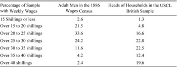
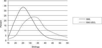
A number of writers have attempted to investigate the extent to which the USCL survey was representative of workers in Britain in the 1890s. Lees examined the budgets of the sub- sample of 777 English households and found that more than one-half worked in the cotton and wool industries (52 percent) and that skilled workers “predominate.” Lees thought that “While the sample is clearly biased away from the unskilled, from the transient, the irregularly employed, and the youngest workers, it clearly reaches far beyond an aristocracy of labor” (Ibid, p. 171). Further work on the biases of the USCL sample of British households was carried out by Hatton, Boyer, and Bailey (Reference Hatton, Boyer and Bailey1994). They found that of the 956 workers considered, 263 were unskilled, 409 semi-skilled, and 284 were skilled. However, this categorization varied across industries such that “unskilled workers form the dominant group in pig iron and coke; semi-skilled workers the dominant group in cotton, wool and coal; and skilled workers the dominant group in steel, bar-iron and glass” (Hatton, Boyer, and Bailey, p. 440). Looking at average income by industry, therefore, gives a misleading impression of the hierarchy of high- and low-wage industries. This point was further investigated by Horrell and Oxley (Reference Horrell and Oxley1999). In a comparison of the average income figures recorded in the USCL budgets with other data available for earnings in the industries, they found that although the male earnings were “in line with those for their occupations, the budgets oversample from the higher-paying occupations in each industry and the distribution of earnings for the whole sample thus falls into a higher range than that found for the industry as a whole” (Ibid, p. 499). Table 1 and Figure 1 illustrate Horrell and Oxley's point. They compare the distribution of recorded earnings in 1890–1891 with the 1886 wage census and show the extent to which the USCL likely oversamples heads of households with relatively high weekly earnings.

Table 1

WAGE DISTRIBUTIONS FROM THE 1886 WAGE CENSUS AND THE USCL HEADS OF HOUSEHOLDS

Sources:

Calculated by authors from the 1890–1891 United States Commissioner of Labor Data and 1886 Wage Census British Parliamentary Papers 1893–1894 [C.6889] “Wages. General report on the wages of the manual labour classes in the United Kingdom,” p. 476.

There is compelling evidence, therefore, to suggest that the workers sampled in USCL were not only engaged in heavy manual work but were also mostly in the higher-income part of the British wage distribution. For instance, the mean USCL wage of more than 31 shillings is in the top 20 percent of the 1886 wage census distribution.Footnote ⁵ This sampling has implications for Logan's findings. If these workers were heads of hungry households, then it is likely the households headed by lower-paid workers were on average even hungrier and very close to seriously inadequate diets.

Figure 1

BRITISH WEEKLY EARNINGS DISTRIBUTIONS FOR ADULT MEN IN 1886 WAGE CENSUS AND IN USCL

Sources: Calculated by authors from the 1890–1891 United States Commissioner of Labor Data and 1886 Wage Census British Parliamentary Papers 1893–1894 [C.6889] “Wages. General report on the wages of the manual labour classes in the United Kingdom,” p. 476.

CALCULATING AVAILABLE CALORIES IN THE USCL DATA

The food section of the USCL survey asks respondents to give an itemized expenditure “of a year's living.” This was, in turn, aggregated to expenditure on more than 20 categories of food and converted to U.S. dollars. This level of aggregation is quite high and raises problems for the conversion of expenditures into quantities and calories. There are, however, some relatively homogeneous food categories for which the questionnaire asked for food quantities, mostly for items that tended to be sold by a standard weight. As we explain later, these include all the key foodstuff for calories, so the seemingly daunting problem of aggregation, for example of all fruit and vegetables, turns out in practice not to be a major problem for our purpose. From the point of view of calorie estimation food expenditure aggregation raises two issues: the choice of deflator to a unit of weight and the choice of conversion into calories.

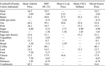
Logan constructed prices to deflate budget expenditures for each of the food categories, by taking the average of the reported British prices for foods in the Aldrich Report (U.S. Senate Committee on Finance, 1892).Footnote ⁶ The example he uses is the case of butter, of which two types, creamery and dairy, were recorded and these were averaged to create the butter price (Logan Reference Logan2006, p. 317). The British prices themselves were collected from a limited number of stores in Leeds, Manchester, and Liverpool in June of 1889. The averages taken from the Aldrich Report are listed in the first column of Table 2. These, however, are not the only prices available. To reach a broader view of the validity of the Aldrich prices, prices are taken from two alternative sources. The USCL survey collected both expenditures and quantities purchased for some foods. The mean implicit deflator from USCL is presented in the second column of Table 2. The most important external source comes from the British Parliamentary Papers (BPP), House of Commons Report on wholesale and retail prices for 1903 (BPP HC.321, 1903). This reports time series of retail prices for a large number of food types, often differentiated by quality and place of sale although many are retail prices from London stores (presented in column 3).

A second important source of important food prices is the Labour Gazette that regularly published prices from Co-op stores around the country. These are listed in column 3. The fifth column of Table 2 gives our “best” set of prices, which are the USCL deflators where we have them with gaps filled in from the BPP HC.321 column.Footnote ⁷ Bread, flour, butter, pork (particularly bacon), sugar, meat, and potatoes are the key foodstuffs for calories in this sample for nutrition. For flour, butter, and sugar the “mixed source” price is above our Aldrich price, while for bread and pork the reverse is true and for meat the prices are identical. It is relevant that all price differences for these energy-important foodstuffs are less than 5 percent. As a consequence, the estimated quantities—and hence our estimates of energy available from the diets—are not significantly affected by these price differences.

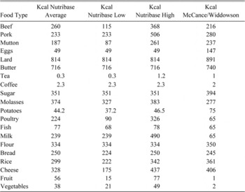
To convert from quantities to calories, we take calorie values from Nutribase (2001) as did Logan (Reference Logan2006, Reference Logan2009). This source is encyclopedic and gives nutrition data for a vast array of foods. For instance, it offers more than 350 types of bread, with wide variation in calorie estimates. The approach taken here is to sample from Nutribase by food category, and then use the mean calories from our sample as well as, where possible, values that are plus or minus two standard deviations from the mean. These estimates are given as the first three columns of Table 3. The fourth column is from the British standard source of nutritional information, commonly referred to as McCance and Widdowson (Paul and Southgate Reference Paul and Southgate1979).

Table 2

COMPARISON OF US¢ PRICES USED FOR CONVERSION OF EXPENDITURE TO QUANTITY

Sources:

For retail prices in Table 2:

• (a) Column 1: U.S. Senate Committee on Finance. Retail Prices and Wages: A Report by Mr. Aldrich…

• (b) Column 2:

  • Bread: BPP, HC.321 1890 large firm price (from Baker's Record), p. 223.

  • Butter: HC.321 mean of Danish and Irish Butter London quarterly prices 1890, Firm A, p. 285.

  • Cheese: HC.321 weighted average of home-produced Cheddar (0.75) and imported American and Canadian cheese (0.25); 1890 price Firm A, p. 290.

  • Coffee: HC.321 mean of Mocha roasted and ground, Costa Rica ground; London price 1890 Firm A, p. 330.

  • Eggs: HC.321, mean of quarterly prices for new laid eggs, 1890, Firm A, p. 297.

  • Lard: HC.321, mean of London price of Lard 1890, Firm (by block per pound) A and Firm D (per packet per pound), p. 278.

  • Fish: HC.321 commences 1898. Mean of quarterly London price for Haddock and whole Cod, Firm A, p. 298.

  • Note that the price of preserved Salmon was 7.5d/pound in 1891 (Firm A, p. 300).

  • Fruit: Prest (Reference Prest1954) average price 1900 of apples and pears, Table 32 p. 60.

  • Flour: HC.321 mean London 1890 price of household flour per seven pounds, Firm A and Firm D, p. 236–7.

  • Pork: HC321 mean London 1890 price of three cuts (belly, chops, legs), Firm A, p. 272.

  • Meat (assumed to be mutton): HC.321 weighted average 1890 March and September price of four cuts of British

  • Mutton (0.75) and eight cuts of imported New Zealand Mutton (0.25), price Firm A, p. 268–9.

  • Sugar: HC.321 average of 1890 London prices for Demerara and granulated sugar Firm A and C, p. 304 and 306.

  • Tea: HC.324 average of 1890 London prices of three types of China and three types of Indian tea Firm A, p. 325.

  • Vegetables: Prest (Reference Prest1954) average of 1900 price for cabbage, beans, peas, turnip, carrot, and onions. Table 29, p. 52.

  • Condiments: HC.321 average of 1890 London price of vinegar (Firm C per quart bottle) and ground black pepper per pound (Firm A), p. 339 and p. 340.

  • Beef: HC.321 average of 1890 London prices (March and September) for 5 cuts of meat, Firm A p. 260.

  • Potatoes: HC.321 average of 1893–1894 price for potatoes Firm A (number of pounds per 12d), p. 259.

  • Rice: HC.321 average of 1890 London price per two pounds for five types of rice (Firm A), p. 240.

  • Molasses: HC.321 average 1890 London price per two pound tin for golden syrup dark and light, Firm A p. 308.

  • Milk: HC.321 average 1890 London “prevailing retail price,” p. 279.

• (c) Column 3: Co-operative store prices (average of 91 societies, 1893), The Labour Gazette, August 1893, p. 88, for Bread, Butter, Cheese, Bacon, Flour Sugar, Tea, Potatoes, Milk and Fresh Meat. The Gazette also lists the price of Margarine and Jams/Marmalade, which have not been used.

• (d) Column 4: Authors’ calculations from USCL data.

Table 3

CALORIES AVAILABLE BY FOOD, PER 100G, FROM NUTRIBASE AND MCCANCE AND WIDDOWSON

Sources:

Nutribase (2001) and Paul and Southgate (Reference Paul and Southgate1979). See text from method of calculation.

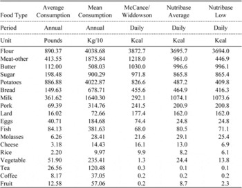
There are some notable differences between these sources. The mean Nutribase values are lower than the McCance and Widdowson values for meat, eggs, and cheese and a lot higher for milk.Footnote ⁸ Table 4 provides estimates of annual average household consumption of each food type. Column 1 reports average consumption (in pounds) derived from reported quantities in USCL survey reports, where available, and otherwise from the expenditure data deflated by the appropriate retail prices given in BPP HC.301.

In column 2 we convert average annual consumption to units of 100g and in columns 3, 4 and 5, these figures are used to derive daily household energy estimates using the Nutribase average, Nutribase low, and McCance and Widdowson nutritional values. For those foods that are recorded separately, the importance of bread (baked and as flour) and butter in the diet is instantly visible in Table 4. Moreover, because the energy conversion factors of these items do not vary too much by source, the broad calorie story is almost the same for whichever conversion is used.Footnote ⁹ One further aspect of the survey is worth noting here. Respondents were asked to estimate how much they spent of “other foods.” The answers ranged from zero (for more than 20 percent of households) to 30 percent of all spending in one particular case. For almost 94 percent of all households the share of other foods was 10 percent or less, and the average share was 3.6 percent. It is possible meals eaten outside the home accounted for some of this spending, and also some low calorie purchases like condiments and vinegar. We decided simply to gross up our calorie estimates by the expenditure share of other foods. If we are correct on the possible kinds of expenditure reflected in this spending, then we might induce a small upward bias into our calorie estimates, since meals taken outside the home would have been relatively expensive and condiments contain few calories.

Table 4

AVERAGE ANNUAL CONSUMPTION PER HOUSEHOLD

Source:

Authors calculations from the data on British households in the USCL data set.

Table 5

MEAN DAILY CALORIES AVAILABLE, PER CAPITA, ESTIMATES, ALL USING STONE PRICES (For reference, Logan (Reference Logan2006, Reference Logan2009) estimates a mean of 1,390 Kcal)

Notes:

The terms in brackets in the second and fourth columns and standard errors.

Source:

Authors calculations from the data on British households in the USCL data set.

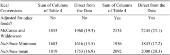
Per capita daily calorie intakes are estimated in several ways and presented in Table 5. In columns 1 and 2 no adjustment is made for “other food,” while that adjustment is made in columns 3 and 4. Column 1 is the sum of all foods reported in Table 4, using different nutritional conversions, divided by the mean household size. The energy values reported in column 3 inflate this total by food expenditure on other foods as a proportion of total food expenditure. This method treats these unspecified other foods as nutritionally equivalent to the average value of all specified foods. Totals are reported with and without this adjustment. Columns 2 and 4 report estimates directly from the household data, so these are the sample mean per capita daily calorie estimates, with standard errors attached. In principle the two numbers should be identical. However, the mean calorie numbers in Table 4 and thus in columns 1 and 3 of Table 5 are from all available observations, rather than observations where estimates for all foods are present, which is the case from columns 2 and 4 of Table 5. Whichever method is used to calculate the nutritional value of the diets of British households in the USCL survey, these estimates of available energy per capita are much higher than Logan's.

Our best estimate is that the energy available to the British urban households included in the USCL survey was around 2,000–2,200 kcal per capita per day, or 2,600–2,900 kcal per equivalent adult man, excluding calories from alcoholic drinks. This is about 50 percent above Logan's estimate, of less than 1,400 kcal per capita per day, from the same source. If we were to add energy from alcohol consumption, it would probably raise our estimate by about 400 kcal (see Gazeley and Newell Reference Gazeley and Newell2012, p. 17).Footnote ¹⁰ We note that this preferred estimate also is similar to Gazeley and Horrell's recent findings for the energy available to agricultural laborer's households of 2,153 kcal per capita per day in 1893–1894, which already includes some allowance for energy from alcohol (Gazeley and Horrell Reference Gazeley and Horrell2013, p. 12).

If we consider the comparison between Britain in 1890 and Maharashtra in the early 1980s, recall that Logan (Reference Logan2009) suggests the households of some of the better-paid British workers around 1890 had many fewer calories at their disposal than rural families in Maharashtra in the early 1980s. This result stems from the particularly low calorie conversion in Logan's work. There are two other aspects of the comparison that suggest the reverse relativity. The first one stems from the finding that in both the USCL and the Maharashtra samples, the price of calories purchased in the form of meat was around ten times that of calories purchased in the form of cereals.Footnote ¹¹ Among the Maharashtrian households, expenditure on meat was on average about 5 percent of total food spending (Subramanian and Deaton Reference Subramanian and Deaton1996, Table 1). In the USCL sample, by contrast, the share of meat expenditure was more than five times larger on average, at 25.5 percent. Making any reasonable allowance for cultural differences, it is very hard to believe that households with such low levels of available calories as Logan estimates would deliberately make themselves even hungrier by allocating so much of their budget to this most expensive form of energy.

Secondly, Subramanian and Deaton give the mean food share for the Maharashtrian sample at 67 percent; whereas the average food share in the USCL British data is 50 percent, and the Maharashtrian mean food share of 67 percent lies above the 95th percentile of the British sample. The food share is very reliable (inverse) index of economic well-being with a long history (see, for example, Almås Reference Almås2012) and it is unlikely that urban households surviving on very few calories would deliberately devote so few of their resources to food. These comparisons strongly support our higher estimates of available calories among USCL 1890 households.