I. INTRODUCTION
The advent of the Doppler-polarimetric technique for the observation of clouds and precipitation is accompanied by a sharp growth of measurable variables [Reference Yanovsky, Russchenberg, Ligthart and Fomichev1], or measurands. The potential of data interpretation not only becomes higher, but also processing is more complicated. Because of complexity, sometimes it becomes very difficult to implement signal processing in real time that results in a restriction of practical applications of new promising scientific achievements. That is why operative radar data interpretation to derive necessary information arises as a very important problem. A number of Doppler-polarimeteric measurands that together with conventional parameters like reflectivity and Doppler spectrum width can be associated with desired parameters of weather objects. Recently spectral differential reflectivity and other functions and parameters were introduced [Reference Yanovsky, Russchenberg and Unal2, Reference Yanovsky3]. The estimation of such parameters requires rather sophisticated signal processing algorithms. Fuzzy logic and neural network approaches give possibilities to avoid bulky computations and time losses during signal processing, while they can take into account many significant measurands applying the last scientific achievements into the practice. These approaches were successfully applied to such kind of tasks in [Reference Yanovsky, Pitertsev, Ostrovsky, Mazura and Marchuk4] for hydrometeor-type classification and in [Reference Yanovsky, Russchenberg and Ligthart5] for both hydrometeor type and turbulence intensity determination. In this aspect, additional informative parameters are always desirable especially if they carry independent information on the features of the object under study and may increase the functionality, accuracy, and reliability of the system.
In this paper, which is an extended version of [Reference Glushko and Yanovsky6], we study a new Doppler-polarimeteric parameter – differential Doppler velocity (DDV) that was recently introduced [Reference Yanovsky, Russchenberg and Ligthart5–Reference Wilson, Illingworth and Blackman7]. Our goal is to show that this parameter is associated with both rain microstructure and turbulence in rain, and may be useful in meteorological radar as an instrument for hydrometeor-type recognition and turbulence intensity estimation. It can be considered as an additional source of information for remote sensing of atmosphere including fuzzy logic and neural network application to develop radar algorithms for automatic classification of hydrometeor type, turbulence intensity, and dropsize distribution estimation in rain.
Section II of the paper focuses on the phenomenological models of Doppler spectra in the case of reflecting microwave signal from precipitation. It provides math expressions for calculations of spectra at different radar performance specifications including sounding waveform polarization, parameters of the object under study, and conditions of observation.
Section III gives the definition of DDV as a measurable variable that is the subject of investigation.
In Section IV, the software based on the developed models is used for calculations providing theoretical relationship between DDV and the parameters of microstructure of the reflecting object and turbulence intensity.
The results of real data processing for verification and improvement of the theory are presented in Section V.
In Section VI, we point out some applications of the DDV parameter and an example of signal processing prototype working in real time. Finally, we indicate some promising capabilities of the proposed technique and trends of future research.
II. MODELS OF DOPPLER-POLARIMETERIC SPECTRA
It is clear that spectra of the reflected signal can be analyzed by direct Fourier transform with respect to a voltage at the output of radar receiver. However, having a purpose of physical interpretation of measurements during remote sensing, or solving an inverse problem, it would be extremely important to build a model of the expected spectrum that would be based on a phenomenological consideration respective to the critical properties of the object under study as well as the frequency band and other features of microwave facility that is used for remote sensing. This section describes such a model based on the approach [Reference Yanovsky3] and suitable for DDV calculations.
The basic initial models that are necessary for theoretical consideration are the models of: (a) microstructure of scatterers in resolution volume of rain; (b) turbulence that may affect the scatterers; (c) inertia of raindrops, which do not follow turbulence motion perfectly; (d) coordinates and polarization basis.
The microstructure of rain is described by generally accepted Gamma dropsize distribution (DSD) in the form [Reference Doviak and Zrnic8]

where N(D) is the number of droplets with an equivalent diameter between D and D+dD in the unit of volume, D 0 is the diameter of the median drop volume. Expression (1) includes the Marshall–Palmer model as a special case for μ = 0. In the case μ ≠ 0, N 0 can be derived [Reference Yanovsky3] from the Marshall–Palmer distribution by keeping the rainwater content constant for a given D 0. The fall speed of raindrops in stationary air is related to their size. The approximation of the relationship between drop diameter D and the drop fall speed is given in [Reference Atlas, Srivastava and Sekhon9]. We just take into account antenna elevation angle θ to obtain a radial component v f of drop fall velocity:

The shape of a droplet is described by the axial ratio ρ = a 3/a 1, where a 1 and a 3 are horizontal and vertical semi-axes of the spheroid as a model of droplet shape, and the following [Reference Yanovsky3]:
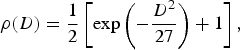
where D is the equivolumeteric droplet diameter in mm.
Turbulence is modeled by its energetic spectrum according to Kolmogoroff–Obukhoff minus five third law [Reference Tatarski10]:

where ɛ is the eddy dissipation rate, C is the dimensionless constant, Ω is the spatial frequency Ω = 2π/L with L as the turbulence vortex scale, a random value. Model of turbulence (4) supposes a constant eddy dissipation rate ɛ in the inertial sub-range.
Inertia of droplets was taken into account following [Reference Yanovsky3, Reference Yanovsky and Fishman11]. Bigger drops are more oblate, they fall faster and contribute more to the reflectivity, but they are more inertial and less involved in turbulent motion than small droplets.
Linear orthogonal polarization basis was used. Polarization of radar signal depends on antenna orientation or, more exactly, on spatial direction of wave propagation. ‘Horizontal’ polarization (ϕ = 0) is really horizontal (E-vector lies in the horizontal plane independently on elevation angle θ); the position of vector E at ‘vertical’ polarization (ϕ = π/2) depends on the elevation angle θ: it is really vertical at horizontal sounding, it is horizontal at the sounding into zenith.
Considering the Doppler-polarimetric approach, one should take into account that Doppler measurements give information about radial velocities of the hydrometeors, while polarimetry is connected with the shape and orientation of the hydrometeors. In the frequency domain, the Doppler-polarimetric radar is able to measure Doppler energy spectra at different combinations of polarizations of transmitted and received waves, so-called Doppler-polarimetric spectra.
Theoretically, the Doppler-polarimetric spectrum is proportional to the drop radial velocity distribution weighted by reflectivity and number of droplets with a given diameter in the unity of resolution volume. It can be written down as

where p(v/D, ɛ, θ) is the radial velocity distribution under the condition of drop equivolumetric diameter D that is moving due to gravity and turbulence with eddy dissipation rate ɛ at antenna elevation equal to θ;
σmn (D/θ, ɛ) is a radar cross-section (RCS) of the non-spherical droplet of given equivolumetric diameter at θ antenna elevation and ɛ turbulence intensity for mn polarization (m = h;v, n = h;v). In case λ ≫ D RCS is [Reference Yanovsky, Russchenberg and Unal2]:

where F mn (Λ) and Φmn(δ, α, θ) represent the shape of the particle (quantified with Λ) and orientation (δ, α) of the droplet; ɛr characterizes the relative electric permittivity.
Probability density of droplet velocity caused by turbulence can be calculated as done in [Reference Yanovsky, Russchenberg and Ligthart5]:

with w T as probability density of turbulence velocity and w(L) as probability density of spatial scales of turbulence. The lower limit of the integration L thres in formula (7) is a minimal (threshold) spatial scale of vortex, which involves a raindrop into the turbulent motion. It is a function of drop diameter D.
Integration over D gives drop turbulent velocity distribution (DTVD) – DTVD of an ensemble of droplets:
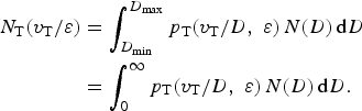
The limits of integration can be taken from 0 to infinity, if N(D) = 0 at D < D min and D > D max. The last inequalities are true practically.
Radial velocity distribution p(v) caused by both turbulence v T and gravity v f can be calculated if one takes into account that v = v f + v T and partial distribution (for specific droplet diameter) can be written as p T [(v − v f)/D, ɛ]. After integration over all diameters of drops, one can obtain a non-normalized distribution of velocity for ensemble of drops:

and then the probability density after normalization is

As follows from (1), (2), and (7), both functions p Σ(v) and p(v) depend also on θ, ɛ, D o, μ and some other values, which can be used as parameters during calculations; they are not indicated directly in expressions (9) and (10) for simplicity.
Finally, Doppler-polarimetric spectra at any combination of sounding waveform polarization and co- or cross-polarization component on reception can be calculated under different conditions by substituting (10), (6), and (1) into expression (5).
III. MEASURABLE VARIABLES AND DDV DEFINITION
There are a number of measurands typical for polarimetric weather radar, such as [Reference Doviak and Zrnic8] differential reflectivity ZDR, linear depolarization ratio LDR, co-polar correlation coefficient between orthogonally polarized signals ρ, specific differential phase Kdp. Some new measurable parameters were studied in [Reference Yanovsky, Russchenberg and Unal2], particularly spectral differential reflectivity is defined as sZdr = 10 lg[S hh(v)/S vv(v)] with S hh(v) and S vv(v) as Doppler spectra estimations at horizontal (hh) and vertical (vv) polarizations. For circular polarization, the resembling parameter was proposed earlier in [Reference Kezys, Torlaschi and Haykin12]. Another parameter EPS can be called ‘equivalent eddy dissipation rate.’ It is calculated from the observed Doppler spectrum width by subtracting a contribution of drop fall distribution component by using the algorithm described in [Reference Yanovsky, Russchenberg and Unal2].
Having an expression for Doppler-polarimetric spectra, the mean Doppler velocity is calculated as the first ordinary moment of a corresponding spectrum. Finally, DDV can be defined based on the expressions for Doppler-polarimetric spectra (5) as

Expression (11) is a platform for the calculation of DDV at different conditions.
In rain, the bigger drops are more oblate and they fall faster than smaller drops. Moreover, bigger drops contribute more to the mean value of Doppler velocity at horizontal polarization than at vertical polarization due to normal orientation of oblate raindrops with horizontal bigger axis of spheroid [Reference Doviak and Zrnic8]. That is why DDV appears as a positive or close to zero value in case of rain. It should depend also on antenna elevation angle θ, eddy dissipation rate ɛ, and parameters of DSD N(D): median drop diameter D 0 and spread μ.
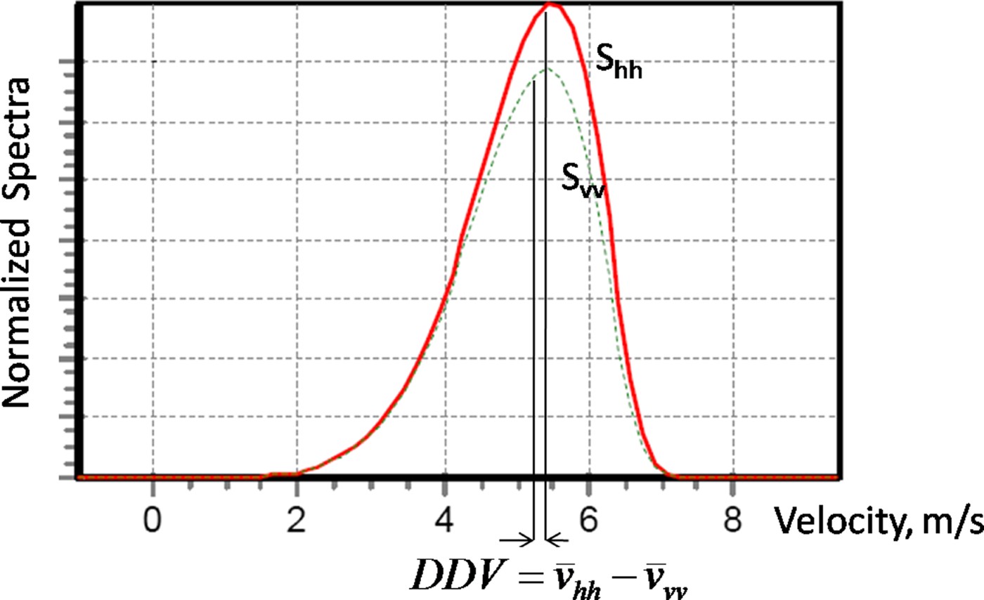
Figure 1 Doppler spectra of raindrops at horizontal (S hh) and vertical (S vv) polarizations calculated at gamma drop size distribution (DSD) with median drop diameter 1.5 mm, antenna elevation θ = 45° and negligible turbulence (ɛ = 0.0001 m2s3). Parameter ΔV is indicated as the difference between mean velocities at orthogonal polarizations.
Demonstrates an example of Doppler spectra of rain calculated at horizontal and vertical polarizations.
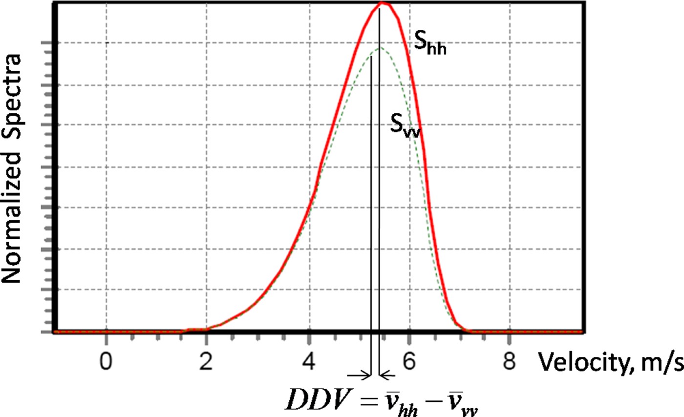
The actual difference between mean Doppler velocities  hh− vv varies with elevation angle θ. In order to eliminate dependence on the viewing angle (antenna elevation θ), DDV can be defined ΔV/sin θ [Reference Wilson, Illingworth and Blackman7]. In [Reference Wilson, Illingworth and Blackman7], it was shown that DDV depends on DSD. In [Reference Yanovsky, Russchenberg and Ligthart5], the dependence between DDV and turbulence intensity was supposed.
IV. DDV CALCULATIONS
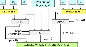
The software developed earlier [Reference Yanovsky3] was modernized to calculate DDV as a function of microstructure and wind parameters. The structure of the software is shown in Fig. 2. Input data are: (i) parameters of gamma DSD, namely, spread factor μ and median drop diameter D 0 (third parameter – scaling factor N 0 is dependent and calculated by the software); (ii) viewing angle or antenna elevation θ; (iii) polarization model as linear polarization radar waveform that can be set as ‘horizontal’ or ‘vertical’ on transmission and reception forming hh, vv, and hv (vh) combinations; (iv) parameters of wind and turbulence model, namely, average wind speed W, eddy dissipation rate ɛ, and turbulence outer scale [Reference Tatarski10] limitations L out, that is, the largest vortex scale L taken into account.
Structure of the software developed to calculate DDV as a function of microstructure of rain and turbulence parameters.

The developed software forms DSD and turbulence models. Then the drop fall velocity distribution and the DTVD are developed taking into account the inertia of droplets of different sizes. These data allow getting statistical characteristics of scatterers (droplets) motion in reflecting volume. After integration with weighting by RCS of drops, the developed software calculates Doppler spectra at different polarimetric parameters S hh(v), S vv(v) and DDV for various initial parameters of DSD, turbulence, etc.
A) Relationship of DDV with microstructure of precipitation
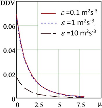
Having these Doppler spectra, one can easily investigate the behavior of DDV under the different conditions and its relationship with microstructure of rain given by DSD initially. Such numerous calculation results have been analyzed. Figure 3 shows the dependence between DDV and one of the microstructure parameters – spread of Gamma DSD μ.
DDV curves as a function of spread parameter μ of Gamma DSD model. Calculations were done at D o = 2.0 mm and three values of eddy dissipation rate ɛ indicated as numbers in (m2/s3). The solid curve corresponds to ɛ = 0.1 m2/s3, dotted curve – ɛ = 1 m2/s3, and dashed curve – ɛ = 10 m2/s3.

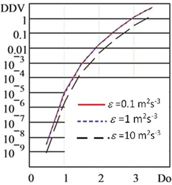
One can see from Fig. 3 that broadening DSD (increasing μ) leads to decreasing DDV, and this phenomenon affects more if the turbulence intensity is higher. These calculation results are improved by the investigation of the median droplet diameter D 0 influence onto the DDV behavior. Median drop diameter is the second important parameter of Gamma DSD and can be reliably associated with rain rate. These results are given in Fig. 4, where three curves represent different eddy dissipation rate values at the same μ = 2.
DDV curves as a function of median drop diameter D o as a parameter of the Gamma DSD model. Calculations were done at μ = 2.0 mm and three values of eddy dissipation rate ɛ indicated as numbers in (m2/s3). The solid curve corresponds to ɛ = 0.1 m2/s3, dotted curve – ɛ = 1 m2/s3, and dashed curve – ɛ = 103m2/s3.

One can see that solid and dotted curves in Fig. 4 almost coincide. This fact means that light turbulence practically has quite minor impact on DDV as a parameter that characterizes the microstructure of the object under study.
The relations between DDV as a measurable variable and DSD as desirable data are really strong in the case of absence of turbulence. Bigger values of median drop diameter D o definitely increase positive DDV values. Broadening DSD (increasing μ) leads to decreasing DDV. That is why the observed DDV values together with such common polarimetric parameter as ZDR = 10 lg(Z hh/Z vv) – differential reflectivity can be used to derive all DSD parameters:D 0, μ, and scaling parameter N 0, especially if reflectivity Z is also estimated (no matter Z vv or Z hh).
B) Relationship of DDV with wind and turbulence parameters
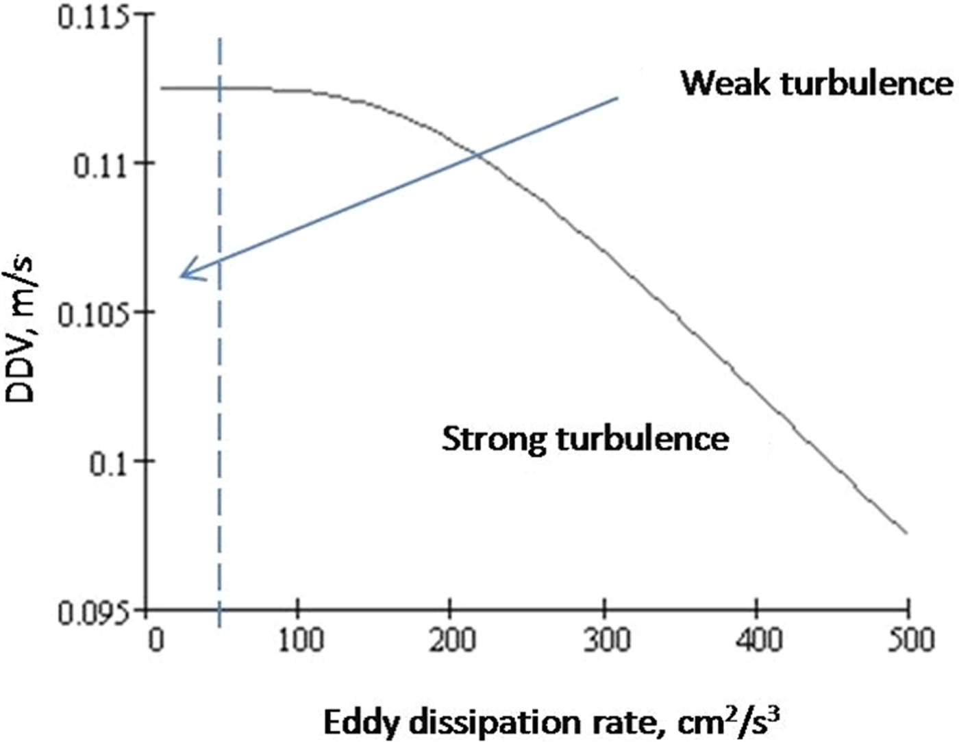
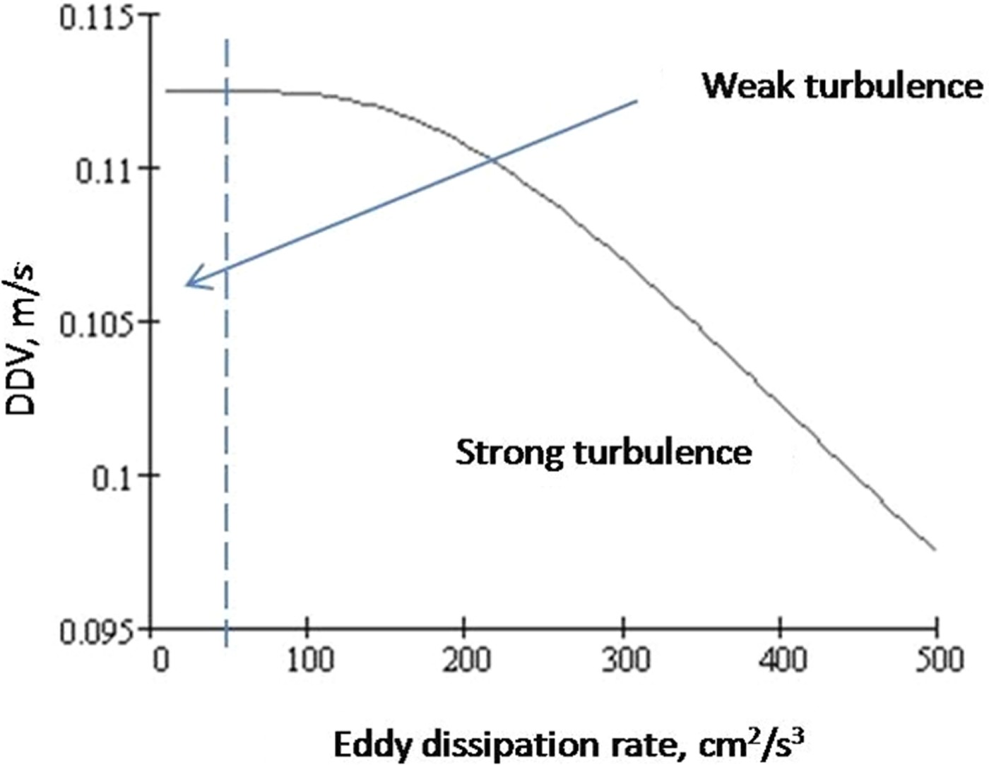
Turbulence tends to smear out the details of the actual Doppler spectra observed. The calculations show how it has an influence upon the difference in the mean values of velocity using horizontal and vertical polarizations. In case of light turbulence, DDV is slightly affected. However, strong turbulence influences significantly. This is illustrated by the result of calculation in Fig. 5.
Results of calculation: DDV versus eddy dissipation rate at θ = 30°, D 0 = 1.5 mm, and μ = 5.
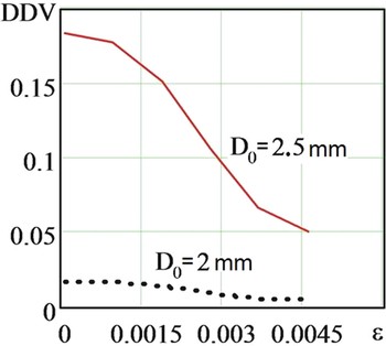
Particularly, DDV values as a function of the eddy dissipation rate and similar microstructure parameters are presented in Fig. 6.
DDV curves as function of eddy dissipation rate ɛ (m2/s3). The solid curve corresponds to D o = 2.5 mm and dotted curve corresponds to D o = 2.0 mm.

It is seen from the figure that under the action of turbulent air motions, DDV decreases with an increasing eddy dissipation rate. Median drop diameter D 0 is strongly related with the intensity of rain, and larger droplets provide higher DDV values.
V. MEASUREMENTS
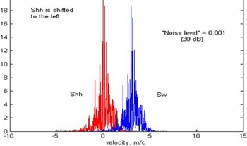
Measurements were done by using the Doppler-polarimetric Transportable Atmospheric Radar (TARA) of the Delft University of Technology (TU-Delft), The Netherlands. TARA is S-band CW FM radar with high resolution. Particularly the mode of 15 m range resolution was used during the observations of widespread and continuous rain including the melting layer and the ice part of a cloud in Cabauw Experimental Site for Atmospheric Research, located in the center of the Netherlands. Raw data were saved in 2001 and dedicated data processing was done recently in Kiev. Figure 7 represents an example of non-averaged sampling Doppler spectra measurements that can be compared with the calculation presented in Fig. 1.
Measured sampling Doppler spectra S hh(v) and S vv(v). The image S hh(v) is shifted to the left for better visual discrimination between the spectra.

In rain, DDV was always positive and had a value of 0.03–0.2 m/s taking into account adjustment on antenna elevation θ. Positive DDV in rain was expected due to the normal orientation of raindrops which are oblate. Estimates of μ showed the most frequent values in rain of 5 and 6, but they vary substantially. Within the melting layer DDV becomes negative, with a value of around – 0.05–0.25 m/s. This can be explained by the fact that the faster-falling rain drops are more spherical than slow snowflakes and suchlike. DDV values (absolute magnitudes) in the ice part of the cloud are normally noticeably less than in rain or the melting layer. This can occur, because the spread in fall velocities of ice particles is much less than that of raindrops and a fortiori of a mixture of drops and snowflakes.
These results are in good coordination with the developed theory [Reference Yanovsky, Russchenberg and Ligthart5] as well as with experimental data of Wilson et al. [Reference Wilson, Illingworth and Blackman7]. That means that parameter DDV, which can be easily measured in real time, can be used operationally for estimation of DSD in rain as well as for hydrometeor-type recognition as an additional measurand.
A uniform wind should have no effect on the measurement of DDV, since both estimates of Doppler velocity are affected by the same speed of air as was pointed by Wilson et al. [Reference Wilson, Illingworth and Blackman7]. The situation that needs to be considered is related to a wind shear or turbulence within the pulse resolution volume. Metcalf [Reference Metcalf13], who analyzed the difference in various Doppler velocities, measured using circular polarization, concentrated on looking for the effect of high wind shears, which can affect the Doppler velocities of different fall speeds of particles.
In case of linear polarization, wind shear influence on DDV was investigated by Wilson et al. [Reference Wilson, Illingworth and Blackman7]. One of the reasons why wind shear should affect DDV relates to a horizontal wind shear [Reference Metcalf13], when the larger particles take longer to respond to the wind change, so their horizontal velocity is not that of the wind. Hence, the horizontal velocity at a given height will depend on the fall speed of the particles. Such shear effect is most severe at higher terminal velocities, as would occur in rain. Ice has much lower fall speeds, so even in strong wind shears this effect is negligible. This shear effect is independent of the beam width and decreases with increasing elevation angle.
Another reason, pointed out by Wilson et al. [Reference Wilson, Illingworth and Blackman7], relates to a shear that exists together with a change in the type of particle across the pulse resolution volume. This could occur, for example, at the bottom of the melting layer, and then the measured DDV values could be biased. The narrower the width of the beam, the lesser such wind shear influence is. Anyhow in case of strong wind, shear measurements of DDV in rain can be biased.
The independence of DDV on turbulence intensity was supposed in [Reference Wilson, Illingworth and Blackman7]. In contrast, our research shows that DDV is negatively correlated with turbulence intensity. This effect should be taken into account when using DDV as measurable parameter for deriving information about microstructure rain. Moreover, it can be considered as one of the measurands in the system estimating turbulence intensity and especially hydrometeor-type recognition.
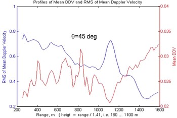
It is interesting to compare DDV behavior with other parameters that are derived from the same raw data. As an example, profiles of mean DDV and rms of mean Doppler velocity are shown in Fig. 8.
Profiles of mean DDV and rms of averaged Doppler velocity at inclined sounding (45°) in light rain. Horizontal axis presents the range.

One can see that the trend of the DDV is opposite to that of the rms of the mean Doppler velocity. This illustrates a kind of negative correlation.
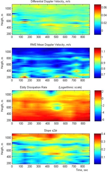
In the images, given in Fig. 9, measurement results are shown in coordinates ‘Height–Time’. They compare the field of DDV with other measurable parameters in resolution volumes, particularly: mean Doppler velocity, equivalent eddy dissipation rate, and slope of the linear part of the curve of spectral differential reflectivity (slope sZdr). All measurements were done during about 15 min in widespread rain simultaneously. Color represents the value of the parameter according to the scale given to the right of the image.
Field of DDV in comparison with some other measurable parameters. From the top: DDV; rms mean Doppler velocity; effective eddy dissipation rate; and slope sZdr.

One can see clearly by comparison of these images that DDV behavior tends to be opposite to rms Doppler velocity and turbulence intensity, and to be similar to the slope sZdr – the parameter investigated in [Reference Yanovsky, Russchenberg and Unal2] as a characteristic of turbulence, and which is much more difficult to be measured than DDV.
When analyzing these results, one should take into account that the objects that were sounded (clouds and precipitation) contained only light or negligible turbulence. Moreover, in the image of eddy dissipation rate (Fig. 9) the logarithmic scale was used, and absolute values indicated in the scale are not meaningful, just relative values are important.
Taking into account that DDV is more sensitive to the turbulence intensity in case of strong turbulence (see Fig. 5), it is reasonable to expect an even more pronounced relationship DDV with eddy dissipation rate. This supposition should be checked in further experimental research.
VI. APPLICATIONS
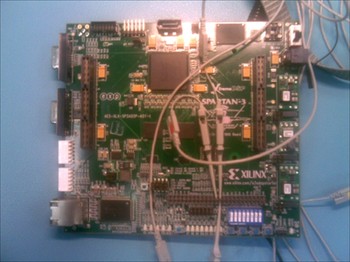
DDV can be used as a perspective parameter for a detailed analysis of microstructure of rain with microwave Doppler-polarimetric radar, and as one of the predictors for automatic recognition of hydrometeor type. It can also be useful for enhancing the efficiency of the remote recognition of hail and icing for aviation purposes. As an example, DDV was used as one of the measurands in the prototype of a weather radar for hydrometeor-type recognition. Fuzzy logic and neural network approach was used [Reference Yanovsky, Ostrovsky and Marchuk14]. In the prototype, in contrast to real radar, the signals are got not from ADC but from PC by USB bus to microcontroller and then to processing device (Fig. 10) based on FPGA Spartan 3 where calculations in real time were done.
The prototype of signal processing device working in real time.

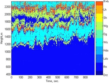
An example of the results of hydrometeor-type recognition by using neural network classifier is presented in Fig. 11. This classifier uses DDV as one of the input parameter together with other measurable variables indicated in section 3. It was trained for recognition between drizzle, rain, low density snow, high density snow, wet snow, graupel, wet graupel; small hail, large hail, and mixture of rain and hail. The same data were used as in the previous paper [Reference Yanovsky, Ostrovsky and Marchuk14].
Result of hydrometeor-type recognition by using real-time neural network classifier. Symbols in color: Drz = drizzle; Rn = rain; Lds = low density snow; Hds = high density snow; Ws = wet snow; Dg = dry graupel; Wg = wet graupel; Sh = small hail; Lh = large hail; R + h = rain + hail mixture.

VII. CONCLUSIONS
In this paper, we have studied radar Doppler spectra of the reflections from rain at different polarizations and in particular the difference between mean Doppler velocities at horizontal and vertical polarizations named DDV.
Theoretical consideration, modeling, and measurements have shown that in the case of microwave radar sounding of rain DDV depends on rain microstructure and turbulence intensity.
Describing drop-size distribution by gamma model, it has been proved that DDV is smaller if spread parameter μ is smaller while DDV increases when median drop diameter D 0 becomes bigger. Turbulence mixing scatterers leads to decreasing DDV values.
DDV can be considered as a novel measurable parameter that is reasonable to be used as an additional source of information for microwave radar remote sensing of atmosphere. Efficiency of DDV application in addition to known Doppler and polarimetric parameters is explained by weak correlation between DDV and other measurands while the correlation between DDV and the parameters of rain microstructure and turbulence in rain is significant.
A prototype of the signal processing device has been developed. Together with other measurable parameters, it uses DDV for fuzzy deriving DSD of rain and hydrometeor-type recognition.
 Dmitry N. Glushko was born in Kiev, Ukraine, on July 26, 1983. He received M.S. degree with Highest Honors in electronics and telecommunications from the Faculty of Electronics of the National Aviation University, Kiev, Ukraine in 2007. From 2006 to 2008, he worked in TTcomm Ukraine (operator of satellite communications) as Technical Manager. In 2008, he joined Radio-electronics Department of NAU as an assistant (teacher) and Ph.D. student. His main research interests are in radar signal processing and remote sensing of the atmosphere. He was awarded Young Engineers Prize for the paper presented at EuRAD-2009 in Rome.
 Felix J. Yanovsky was born in Kiev, Ukraine. He received a radio engineering degree with Highest Honors from Kiev Institute of Civil Aviation Engineers, Ukraine, in 1968, Ph.D. in Radar and Radio-navigation from Moscow State Technical University in 1979. Then he got two D.Sc. degrees: the first one in Aviation Transport/Meteorology from National Aviation University (NAU), Kiev, Ukraine, and the second one in Radar and Radio-navigation from Moscow State Technical University, Russia. For many years he was with the NAU in Kiev, Ukraine. During 1996–2003; he also worked at the Delft University of Technology, The Netherlands as Top-scientist, Professor. Currently, he is the Head of Radio-electronics Department at NAU. He is an IEEE Fellow, member of Aerospace and Electronics Systems (AES), Geoscience and Remote Sensing (GRS), Microwave Theory and Technique (MTT), and Signal Processing (SP) Societies, and author of more than 400 publications including, 10 books and 40 invention patents. Directions of scientific activity: radar, remote sensing, avionics, signal processing, adaptive measurements, atmosphere electricity, radar meteorology, and Doppler polarimetry.