1 Introduction
In certain shock- and gravity-driven variable-density flows, the memory of initial conditions (IC) remains noticeable as the flow transitions to turbulence (George & Davidson Reference George and Davidson2004; George Reference George2008; Banerjee & Andrews Reference Banerjee and Andrews2009; Kuchibhatla & Ranjan Reference Kuchibhatla and Ranjan2013). Further insight into how the characteristic statistical behaviour of transitional turbulence might depend upon these initial conditions can be provided by studying Richtmyer–Meshkov instability (RMI) (Richtmyer Reference Richtmyer1960). RMI occurs at the interface of two impulsively accelerated fluids, each of different density. RMI is closely related to Rayleigh–Taylor instability (RTI) (Strutt Reference Strutt1900; Taylor Reference Taylor1950), which occurs when a heavy and a light fluid are accelerated such that the density and pressure gradients are oriented in opposite directions, causing growth of initial interface perturbations. Conversely, RMI develops regardless of the relative position of the gases at the interface (heavy/light or light/heavy), and can be considered as an extension of RTI, where the constant acceleration of the interface is replaced by an impulsive acceleration, e.g. a shock which amplifies initial perturbations on the interface. In both instabilities, the vorticity equation for compressible flow is
 $$\begin{eqnarray}\frac{\text{D}\unicode[STIX]{x1D74E}}{\text{D}t}=(\unicode[STIX]{x1D74E}\boldsymbol{\cdot }\unicode[STIX]{x1D735})\boldsymbol{u}-\unicode[STIX]{x1D74E}(\unicode[STIX]{x1D735}\boldsymbol{\cdot }\boldsymbol{u})+\unicode[STIX]{x1D735}\times \left(\frac{1}{\unicode[STIX]{x1D70C}}\unicode[STIX]{x1D735}\boldsymbol{\cdot }\unicode[STIX]{x1D749}\right)+\frac{1}{\unicode[STIX]{x1D70C}^{2}}(\unicode[STIX]{x1D735}\unicode[STIX]{x1D70C}\times \unicode[STIX]{x1D735}P),\end{eqnarray}$$
which highlights the relationship between vorticity and the gradients of density,
 $\unicode[STIX]{x1D70C}$
, and pressure,
 $P$
, showing how the shock deposits baroclinic vorticity at the interface. For large Reynolds numbers, the viscous effect is negligible (
 $\unicode[STIX]{x1D749}$
is the viscous stress tensor). Moreover, upon initial shock, the baroclinic term is dominant over the vortex stretching (
 $(\unicode[STIX]{x1D74E}\boldsymbol{\cdot }\unicode[STIX]{x1D735})\boldsymbol{u}$
) and the vortex dilation (
 $\unicode[STIX]{x1D74E}(\unicode[STIX]{x1D735}\boldsymbol{\cdot }\boldsymbol{u})$
) terms, and therefore the vorticity equation can be approximated by the baroclinic production term (
 $\text{D}\unicode[STIX]{x1D74E}/\text{D}t\approx 1/\unicode[STIX]{x1D70C}^{2}(\unicode[STIX]{x1D735}\unicode[STIX]{x1D70C}\times \unicode[STIX]{x1D735}P)$
). As the initial perturbations grow, vorticity further distorts the interface, and is a primary driving force of RMI evolution. As RMI progresses, it induces turbulence and mixing, making it a phenomenon of interest to a variety of fields.
RMI is an important phenomenon occurring in many applications at length and time scales spanning several orders of magnitude. RMI occurs undesirably at the smallest scales in Inertial Confinement Fusion (ICF) as the ablation, and subsequent shock, of the outer shell material causes mixing with the thermonuclear fuel (Ranjan, Oakley & Bonazza Reference Ranjan, Oakley and Bonazza2011). Experiments have shown that reduced instability growth rates at the shell/fuel interface can improve ICF performance (Lindl et al. Reference Lindl, Landen, Edwards and Moses2014). RMI is equally important at intermediate length scales in applications such as supersonic combustion. In scramjets, the high speed of the aircraft subjects the fuel and oxidizer to multiple shocks in the combustor. A better understanding of RMI could allow for improved design of combustors that optimize mixing for combustion (Waitz, Marble & Zukoski Reference Waitz, Marble and Zukoski1993; Yang, Chang & Bao Reference Yang, Chang and Bao2014; Reilly et al. Reference Reilly, McFarland, Mohaghar and Ranjan2015). On the largest scales, RMI plays an important role in Supernova Remnant (SNR) formation. Although not yet completely understood, there is evidence that RMI may precede or act in conjunction with other instabilities to affect the development of the SNR (Kane, Drake & Remington Reference Kane, Drake and Remington1999; Kifonidis et al. Reference Kifonidis, Plewa, Scheck, Janka and Müller2006).
Understanding the physics responsible for the increase in mixing and turbulent behaviour in these systems begins by recognizing the phenomena driving the production of vorticity. More specifically, the baroclinic production of vorticity at the interface is due to the misalignment of the pressure gradient (provided by the shock) and the density gradients of the two materials. In shock-accelerated flows, the strength of the pressure gradient is indicated by the Mach number of the incident/reflected shock wave. The strength of the density gradient in a two-fluid system is expressed nondimensionally by the Atwood number
 $$\begin{eqnarray}A=\frac{\unicode[STIX]{x1D70C}_{2}-\unicode[STIX]{x1D70C}_{1}}{\unicode[STIX]{x1D70C}_{2}+\unicode[STIX]{x1D70C}_{1}}.\end{eqnarray}$$
In most cases, the subscript 2 refers to heavy fluid while subscript 1 refers to a light fluid. The Atwood number can be used for unshocked and shocked interfaces; however, in the present work,
 $A\sim 0.22$
refers to pre-shock Atwood number. The post-shock and post-reshock Atwood numbers are approximately 0.23 and 0.25, respectively. Initial interface perturbations can be characterized by the ratio (
 $\unicode[STIX]{x1D6FC}=\unicode[STIX]{x1D702}/\unicode[STIX]{x1D706}$
) of their amplitude,
 $\unicode[STIX]{x1D702}$
, to their wavelength,
 $\unicode[STIX]{x1D706}$
. Additionally, this parameter can be related to the growth rate of the overall mixing region, or extent of fluid interpenetration, and essentially defines the misalignment between the interface and the shock (see (1.1)). In the initial growth period, linear growth rates are typically seen for
 $\unicode[STIX]{x1D6FC}<0.1$
, while nonlinear growth rates can be seen earlier for higher
 $\unicode[STIX]{x1D6FC}$
and at later times. In the nonlinear regime, an increase in mixing and tendency toward turbulence are likely. The dependence of RMI upon the density and pressure gradients, which can be directly related to the velocity field, highlights further interest. This linkage signals a departure from passive-scalar mixing, as the variable-density characteristic of the system constantly adjusts the behaviour of the flow in response to forcing from the velocity field (Dimotakis Reference Dimotakis2005).
Many studies have been conducted to better understand the conditions that result in a transition to turbulence. Greater shock strength, higher Atwood number, and larger values of
 $\unicode[STIX]{x1D6FC}$
favour an earlier transition to turbulence. The interaction of the developing interface with a second shock, which can be provided by the reflection of an incident shock at a wall, causes deposition of vorticity on a wider range of length scales. In this way, Balakumar et al. (Reference Balakumar, Orlicz, Tomkins and Prestridge2008) showed the rapid redistribution of previously ordered vorticity, which was believed to drive the mixing region to a turbulent state. Further studies have shown that the modal content of the interface is a key factor for transition. Balakumar et al. (Reference Balakumar, Orlicz, Tomkins and Prestridge2008) showed that the vortex configuration resulting from the initial shock advects material and neighbouring vortices, which strongly affect the extent of the mixing region and the state of the field that interacts with the reshock wave. Weber et al. (Reference Weber, Haehn, Oakley, Rothamer and Bonazza2012) achieved a turbulent mixing transition before reshock for an initial condition consisting of structures with small separation of length scales.
Due to the importance of initial interface perturbations, much work has also been done on the creation and characterization of the initial conditions from which the instability evolves. The first experiments used a thin membrane to separate two gases and prescribe the initial condition (Meshkov Reference Meshkov1969; Brouillette & Sturtevant Reference Brouillette and Sturtevant1994; Vetter & Sturtevant Reference Vetter and Sturtevant1995; Houas & Chemouni Reference Houas and Chemouni1996). However, this technique introduces membrane fragments into the mixing process, influencing instability development as well as complicating flow visualization. Subsequent researchers created membraneless, slightly diffuse interfaces between two gases in vertical shock tubes with heavy gas below light gas. Jacobs & Sheeley (Reference Jacobs and Sheeley1996) used the resulting stable configuration to create a well-defined sinusoidal initial condition between the gases by horizontally oscillating the entire test section.
Several other works in the study of RMI evolution have imposed random-mode initial conditions on an interface. One method creates Faraday waves on an otherwise flat interface, which is achieved by vertically oscillating the column of gases (Jacobs et al. Reference Jacobs, Krivets, Tsiklashvili and Likhachev2013). Other groups have utilized a shearing Kelvin–Helmholtz (KH) type instability at the interface to impose a complex, multi-mode perturbation between the gases. This method allows for the creation of a specific range of initial amplitudes and wavelengths to study the variance of initial conditions on instability evolution and the eventual transition to turbulence (Weber et al. Reference Weber, Haehn, Oakley, Rothamer and Bonazza2012).
Due to the complexity of RMI physics and the typically fast time scales of flow evolution, there have also been many efforts dedicated to understanding RMI using computational methods. As in experimental work, computational studies have concentrated on modeling the instability evolution originating from different initial conditions, while great attention has been dedicated to understanding the evolution from well-defined, two-dimensional, harmonic initial conditions. Furthermore, just as advances in simulations have bolstered RMI experiments, the improvement of experimental diagnostic capabilities have improved the fidelity and breadth of information available for validating and improving simulations. Schilling, Latini & Don (Reference Schilling, Latini and Don2007) performed simulations of single-mode RMI before and after re-shock, and the results were compared to the planar laser induced fluorescence (PLIF) experimental work by Collins & Jacobs (Reference Collins and Jacobs2002), and Latini, Schilling & Don (Reference Latini, Schilling and Don2007) compared dissipation effects using WENO methods of different orders.
McFarland, Greenough & Ranjan (Reference McFarland, Greenough and Ranjan2011) furthered the relationship between experiments and simulations by performing a computational study of RMI development from an inclined interface covering multiple incident shock strengths, initial interface inclinations, and various Atwood numbers using ARES code. The research covered experiments performed on the shock tube which the present work was completed on, and was thus constrained to the capabilities of this facility. Morgan et al. (Reference Morgan, Aure, Stockero, Greenough, Cabot, Likhachev and Jacobs2012) also used ARES code to investigate late-time development of RMI in shock tubes, and later compared with a compressible version of the Miranda code (Cook & Cabot Reference Cook and Cabot2005; Cook Reference Cook2007). The effect of different three-dimensional, multi-mode, small-scale initial perturbations on RMI evolution was previously investigated numerically by Thornber et al. (Reference Thornber, Drikakis, Youngs and Williams2011, Reference Thornber, Drikakis, Youngs and Williams2012) using implicit large-eddy simulation (ILES) with systematic grid refinement which showed the mixing layer transition to a turbulent state.
The modal interactions of the initial conditions investigated in the present study, a large-wavelength inclined interface perturbation and a small-wavelength multi-mode perturbation superimposed on the inclined interface, and their effect on RMI evolution were initially investigated using simulations by McFarland et al. (Reference Mcfarland, Reilly, Black, Greenough and Ranjan2015). These simulations were conducted to directly compare their results with experiments conducted at the facility where the present paper was completed. Thus the conditions (Mach number, gases used, interface inclination angle) in the McFarland study match those of the current study. The study includes an extension to 3D and other improvements upon the work in McFarland et al. (Reference McFarland, Greenough and Ranjan2011), as early simulations differed some in the qualitative results, these simulations encompassed a large range of parametric variations including the perturbation, resolution, and boundary conditions. The ARES work found that before reshock, distinct memory of initial condition was found in both large and small scales. However, as the post-reshock flow proceeded towards turbulence, it only retained some memory of the initial conditions for high-amplitude, large-wavelength perturbations. The results and conclusions of this work have a large influence on the hypothesis of the current work.
The present experimental study aims to address the influence of modal content in the initial condition on RMI transition to a more turbulent state. RMI evolution was studied for two different initial conditions. The first, referred to as the single-mode case (S), is a predominantly single-mode, inclined interface between two gases. It should be noted that the gases are oriented so that the light gas rests on the heavy gas (light/heavy), i.e. the incident shock travels from the light to the heavy gas. The second set of experiments, referred to as the multi-mode case (M), were performed with a perturbed, multi-mode, inclined interface. The imposed perturbation creates density gradients of varying smaller scales, hypothesized to result in various sized density and velocity scales which develop in addition to the major scale of the inclined interface, and do so differently than case S. The initial conditions are described in further detail in the experimental facility section. During the experimental investigation, concentration and velocity fields are obtained by performing instantaneous, simultaneous PLIF and particle image velocimetry (PIV) measurements. RMI evolution has been characterized at two times following the incident shock-interface interaction, and at two different times after the reflected shock (reshock) has interacted with the evolving interface. Quantitative concentration and velocity fields, as well as the coupling of both, are utilized to describe the temporal evolution of the flow and obtain data necessary for achieving the objectives of this study.
The goal of the present study is to further delineate the influence of initial conditions on a transitioning variable-density flow field. Through the statistical characterization of key turbulent parameters we highlight differences and similarities between the single-mode and multi-mode initial conditions. Through the qualitative analysis of the concentration field we provide a highly detailed temporal description of the flow morphology as it transitions towards turbulence. By superimposing vorticity fields onto simulated schlieren images, we highlight the co-location of the density gradients with shear stresses, while also providing further qualitative information about the interfacial evolution. Through a combination of statistics, including turbulent kinetic energy, Reynolds number, and enstrophy, spectral and scalar analysis were used to show that the flow is indeed in a state of transition to turbulence. Obtaining details of how varying initial conditions affect the general mixing characteristics of variable-density flows is also of primary interest to this study.
The current work is presented in the following sections. In § 2, we discuss the experimental facility used to conduct this study and the conditions in which it was completed. Section 3 provides a qualitative analysis of the density fields obtained from PLIF and shows the temporal evolution of the flow field for both experimental cases. In § 4, a quantitative analysis of the PLIF and PIV data is conducted. Section 5 presents the discussion on the flow transition towards turbulence. Finally, § 6 provides the conclusions and discussion for this study.
2 Experimental setup
The experiments were performed at the inclined shock tube facility at Georgia Institute of Technology. The shock tube measures 9 m in total length and has an 11.43 cm by 11.43 cm internal cross section. It is designed to be capable of high incident shock Mach number experiments (
 $M\approx 2.5$
in air at atmospheric conditions). Further explanation of experimental facility can be found in McFarland et al. (Reference McFarland, Reilly, Creel, McDonald, Finn and Ranjan2014b
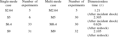
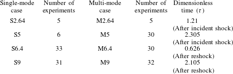
), Reilly et al. (Reference Reilly, McFarland, Mohaghar and Ranjan2015). The experimental duration is 10 ms which is limited by the interaction of the expansion waves from the driver with the interface. Also, the number of realizations selected for each time, experimental times and dimensionless times are given in table 1. Dimensionless times,
 $\unicode[STIX]{x1D70F}=k{\dot{h}}_{0}(t-t^{\ast })$
, are calculated using the method which is described in McFarland et al. (Reference McFarland, Greenough and Ranjan2011) and McFarland, Greenough & Ranjan (Reference McFarland, Greenough and Ranjan2014a
). After incident shock,
 ${\dot{h}}_{0}\approx 17.2~\text{m}~\text{s}^{-1}$
is the initial growth rate, which is measured based on the 5 %–95 % method of computing the mixing width,
 $t$
is the experimental time, and
 $t^{\ast }=\unicode[STIX]{x1D706}/(2w_{i}\tan \unicode[STIX]{x1D703})$
is the time required for the shock wave to traverse the inclined interface. After reshock, the same equation is used; however,
 ${\dot{h}}_{0}\approx 20.7~\text{m}~\text{s}^{-1}$
is the mixing width growth rate after reshock,
 $t^{\ast }=h_{(pre-reshock)}/w_{r}$
is the time that reshock wave traverse the pre-reshock interface,
 $t=t_{exp}-t_{(reshock-interface-interaction)}$
, where
 $t_{exp}$
is actual experimental time and
 $t_{(reshock-interface-interaction)}\approx 5.05~\text{ms}$
.
 $k=2\unicode[STIX]{x03C0}/\unicode[STIX]{x1D706}$
is wave number, and
 $w_{i}$
and
 $w_{r}$
are incident shock and reshock speeds.
Number of experimental realizations selected for analysis per case, experimental times and dimensionless times.
The evolution of the interface was observed with simultaneous PLIF and PIV methods, the results from which were systematically registered to compute the instantaneous density and velocity fields for each experimental realization. The simultaneous measurements were performed by viewing the mixing layer from the same side of the laser plane, which required tilting one of the cameras. It has been verified that one can still obtain a strong PLIF signal even when the camera is tilted and that the perspective calibration preserves the information of the scalar field. A Scheimpflug mount was used with the PLIF camera in order to focus on the off-axis laser plane. This was corrected using calibration images of a dual-plane calibration target and a de-warping algorithm available with Insight 4G™.
PLIF measurements are performed by seeding only the light gas with acetone. In the current study, a Litron laser capable of 120 mJ per pulse at 266 nm is used to illuminate the seeded gas from below. Pure nitrogen is passed through a bubbler held at constant temperature to ensure consistent saturation concentration. The saturated nitrogen is mixed in a large mixing volume with pure nitrogen to achieve a constant concentration of acetone which yields an Atwood number of 0.22 (pure nitrogen/carbon dioxide yields
 $A=0.23$
). The fluorescence emission is captured using an un-intensified TSI PowerView 29 MP CCD camera equipped with a 50 mm f/1.2 Nikon lens with an additional 2+ close up lens. In order to capture only fluorescence emitted by acetone, the camera is equipped with a notch filter removing 532 nm wavelength light due to the PIV signal; 2 by 2 binning is used to increase the signal-to-noise ratio, yielding a spatial resolution of 73
 $\unicode[STIX]{x03BC}\text{m}~\text{pixel}^{-1}$
. Additionally, the acquired images are subjected to further correction to extract the quantitative concentration field (Collins & Jacobs Reference Collins and Jacobs2002; Weber et al.
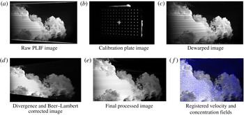
Reference Weber, Haehn, Oakley, Rothamer and Bonazza2012, Reference Weber, Haehn, Oakley, Rothamer and Bonazza2014). A sample image throughout the correction process is shown in appendix A.
For PIV measurements, both gases were seeded with titanium dioxide particles with an average particle size of 0.3–1
 $\unicode[STIX]{x03BC}\text{m}$
. Based on the relaxation time of the particles in either gas, they should fall to no more than 1 % of the current pixel resolution, which is much less than the 10 % subpixel accuracy achieved by the Gaussian subpixel interpolation method (McFarland et al.
Reference McFarland, Reilly, Creel, McDonald, Finn and Ranjan2014b
). The seeded particles were illuminated using a dual-cavity New Wave Research Gemini PIV laser at 200 mJ and wavelength of 532 nm which is diverged into a sheet just before entering the bottom of the tube. The location of the beam waist was adjusted for each image acquisition location, and through a knife-edging technique it was estimated that the laser light sheet thickness at each location was
 ${\approx}0.65\pm 0.05~\text{mm}$
. Acquisition was performed using a TSI PowerView 29-MP CCD camera with a 532 nm bandpass filter and a 2+ close up lens. The two beams of the lasers are combined by reflecting the 266 nm beam and allowing the 532 nm beam to pass through a beam-splitter. The laser sheet thickness was selected based on the depth of field (Stanislas & Monnier Reference Stanislas and Monnier1997):
 $$\begin{eqnarray}\unicode[STIX]{x1D6FF}z\simeq \pm 2.4\bigg(\frac{1-\text{Mag}}{\text{Mag}}\bigg)^{2}\bigg(\frac{f}{2\unicode[STIX]{x1D70E}}\bigg)^{2}\unicode[STIX]{x1D706}.\end{eqnarray}$$
In the present work,
 $f$
-
 $\text{number}=4,\text{Mag}\backsim 0.2,\unicode[STIX]{x1D706}=532~\text{nm}$
, so
 $\unicode[STIX]{x1D6FF}z\simeq \pm 0.33$
, and therefore the illumination of particles outside the depth of field is minimized by keeping the laser sheet thickness approximately equal to the depth of field. Because out-of-plane gradients are present, especially after reshock, the laser sheet thickness and interrogation window are also required to be small in order to mitigate error in the small scales due to the volume-averaging effects associated with PIV (Lavoie et al.
Reference Lavoie, Avallone, De Gregorio, Romano and Antonia2007).
For PIV processing, a combination of grid methodologies are used, a Rectangular Grid engine (pre-reshock) and a recursive Nyquist grid (post-reshock). For the pre-reshock cases, a Rectangular Grid engine is used to enable more control of the grid settings. In addition, in the pre-reshock case, due to the high mean velocity of the flow, an offset of 20 pixels was used to more accurately capture the velocity fluctuations in the moving frame. The image pairs were processed with Insight 4G™ software using a
 $24\times 24$
pixel final spot size with 50 % overlap, which corresponds to a
 $372~\unicode[STIX]{x03BC}\text{m}$
vector spacing. In PIV post-processing, smoothing and interpolation were used. In order to remove the effect of the boundary layers, a mask is used in processing and they are not included in the results, which reduced the interpolated vectors to about 1 % in both experimental cases. In order to reduce the effect of small-scale spurious noise on PIV results, a
 $5\times 5$
Gaussian filter with a standard deviation of 0.8 was used, as it was found to have an acceptably low effect on the small-scale velocity statistics. Concerning the laser synchronization for PIV image capturing, laser pulse time delays of 2.5 and
 $2.2~\unicode[STIX]{x03BC}\text{s}$
were used for the post-reschock and pre-reshock cases, respectively. The details of registering the PIV data with PLIF fields, which is a crucial step in the analysis, are provided in appendix A, and the details of instantaneous and statistical uncertainty measurements are explained in appendix B.
2.1 Initial condition creation and characterization
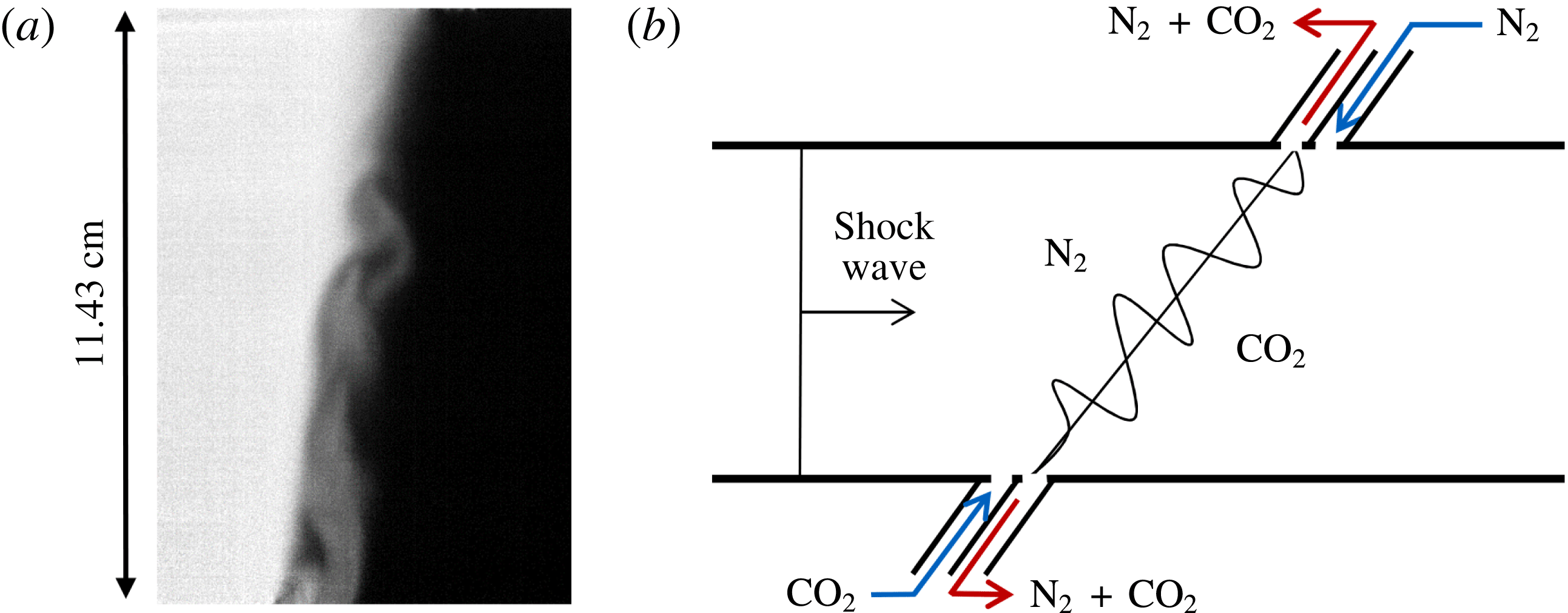
Multi-mode initial condition creation. (a) Sample corrected multi-mode initial condition image where nitrogen is light and carbon dioxide is dark. (b) Simplified schematic showing the general method of interface creation by outflowing the mixture of gases at the interface, shown as red arrows, and flowing pure nitrogen and carbon dioxide below and above the interface, respectively, to create shear and buoyancy effects. In the schematic, the angle of the interface is slightly exaggerated for clarity. In both depictions gravity acts normal to the interface. The actual inlets and outlets consist of small perforations to prevent disturbance of the shock.

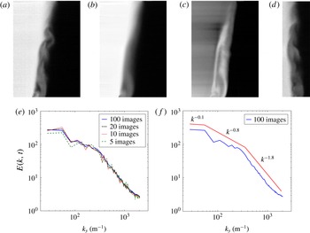
IC characterization: (a) Sample multi-mode IC (image intensity corresponds to mole fraction of nitrogen). (b) Ensemble average of mole fraction for 200 multi-mode IC images. (c) Standard deviation of same 200 images. (d) Multi-mode IC after
 $10^{\circ }$
rotation with respect to inclined shock tube (
 $80^{\circ }$
). (e) Average energy spectra for increasing number of ensemble-averaged images for rotated IC. (f) Energy spectra calculated from a rotated IC in (d) within a concentration between 0.18 and 0.3. Different slopes are shown by red lines.

One of the main goals of this paper is to understand the role of the initial condition in shock-driven, variable-density flows. In order to achieve this goal, we have implemented two sets of initial conditions which vary in their modal composition. The first case is an inclined interface (tube angle of
 $80^{\circ }$
relative to horizon) which is a predominantly single-mode interface. The single-mode interface is created following the process outlined previously (McFarland et al.
Reference McFarland, Reilly, Creel, McDonald, Finn and Ranjan2014b
; Reilly et al.
Reference Reilly, McFarland, Mohaghar and Ranjan2015). It was determined that this method creates a relatively flat interface with a diffusion thickness
 ${\approx}0.96~\text{cm}$
. For insight into the mathematical representation of the inclined interface, which is effectively half of a period of a triangular wave, Mikaelian (Reference Mikaelian2016) suggested that the inclined interface can be closely represented by half of a cosine wave which has a Fourier coefficient carrying 81 % of the Fourier expansion. The multi-mode interface is created by injecting light gas into the heavy gas just below the interface creation plane and by injecting heavy gas into the light gas just above the interface creation plane. The light gas then rises from its injection point in the heavy gas section while the heavy gas falls from its injection point in the light gas section to create a multi-mode interface between the two larger sections of gas. This configuration, combined with the suction of a vacuum pump at the interface outflow slots, creates a counter flow condition with a combination of shear and buoyancy instabilities along the interface. A sample multi-mode initial condition PLIF image corrected for variations in laser intensity and background noise effects is shown in figure 1(a), where the intensity of the image concentration corresponds to the mole fraction of the light gas (white), and the multi-mode interface creation is described in figure 1(b). The initial condition characterization was done by taking 200 PLIF images of the multi-mode interface and then using energy spectra of density and Proper Orthogonal Decomposition (POD) to provide a statistical analysis of the interface.
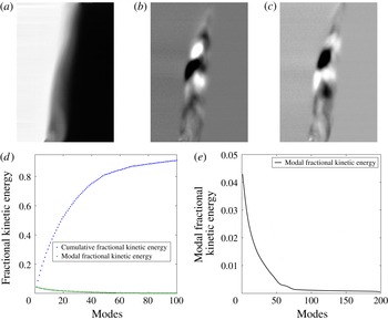
Dominant modes of the POD for 200 ensemble-averaged multi-mode initial conditions and their respective kinetic energy: (a) Mode 0 (Ensemble average), (b) Mode 1 (4.4 % of total kinetic energy), (c) Mode 2 (4.1 % of total kinetic energy). (d) Modal and cumulative fractional kinetic energy for the first 100 (90 %) modes. (e) Modal fraction of kinetic energy for all 200 modes.

Figures 2(b) and 2(c) show the ensemble average and standard deviation, respectively, of the nitrogen mole fraction for 200 PLIF images. As seen in figure 2(c), the largest fluctuation occurred near the bottom surface (the left side of the shock tube) where the mole fraction standard deviation is 1.2 %, which shows the repeatability of our initial condition. In order to isolate the effect of the secondary modes from the large-wavelength inclined perturbation on the energy spectra, images of the inclined multi-mode interface are rotated
 $10^{\circ }$
. One such rotated interface sample is shown in figure 2(d). In a method similar to Weber et al. (Reference Weber, Haehn, Oakley, Rothamer and Bonazza2014), the energy spectrum is calculated along the perturbed region within the concentration between 0.18 and 0.3 (small to mid-range scales), then averaged in the streamwise direction for each realization and then ensemble-averaged for the total number of realizations. Figure 2(e) shows the ensemble average of density energy spectra for an increasing number of interface images, indicating that the spectrum converges after approximately 20 images.
Using 100 images, the ensemble average of energy spectra in the perturbed region is shown in figure 2(f). Three ranges of different slopes can be distinguished from the analysis of the rotated image in figure 2(f). According to figure 2(f), the primary peak wave number is
 $k\approx 40~\text{m}^{-1}$
, and the spectral range that has the highest energy (
 $k<40$
) is related to the shock tube dimension. The spectra undergo a change in slope at
 $k\approx 200~\text{m}^{-1}$
, highlighting an intermediate range from
 $40<k<200$
. The scales in this range relate to shear and buoyancy effects in the initial condition. Finally, the smallest scales, which are related to the diffusion thickness, are seen in a third range (
 $k>200$
), which has the steepest slope of the spectra. Rather than a fit to the data, the figure shows fiducials for the three ranges.
To compute the POD of the initial condition, the same set of 200 PLIF realizations used in the density energy spectra investigation were utilized. In POD, each mode represents a coherent flow structure based on its reoccurrence in all images. Furthermore, to find the kinetic energy of a particular mode, one must look at the associated eigenvalue (Berkooz, Holmes & Lumley Reference Berkooz, Holmes and Lumley1993). In the POD analysis, mode 0 represents the ensemble average of the 200 density fields, as shown in figure 3(a). Additionally, when comparing figure 3(a) with figure 2(b), it can be shown that the images are similar, and thus indicates the accuracy of the POD code used (both of them show ensemble average of flow fields). Although the total, 199, modes in this decomposition were analyzed, to achieve better visualization only the first 90 % of the the modal fraction and cumulative fractional energy of modes are considered, as is shown in figure 3(d). Figures 3(b) and 3(c), respectively, represent modes 1 and 2 of the decomposition, containing 4.4 % and 4.1 % of the total energy, respectively. Figure 3(d) shows that the first 18 modes contain 50 % of the perturbations’ kinetic energy, which suggests multi-mode perturbations are occurring on the interface. To further clarify this point, the modal fraction of kinetic energy is shown in figure 3(e), which illustrates that the first 18 modes comprise a majority of the flow perturbations’ kinetic energy. The connection between POD and energy spectra of density can be observed by considering the mid-range scales in modes 1 and 2 of POD analysis which are approximately
 $2{-}5~\text{cm}$
and are in good agreement with the scales of the intermediate range of energy spectra.
3 Qualitative analysis of time evolution of density fields
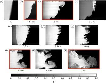
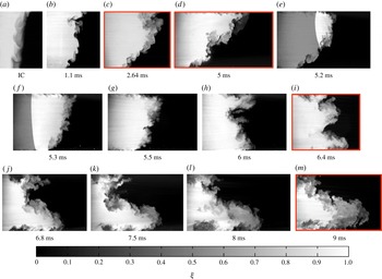
Using several samples of corrected PLIF images, the current section provides a complete temporal evolution of the density fields for both experimental cases. The concentration field evolution for the single-mode case is depicted in figure 4, while the evolution for the multi-mode case is shown in figure 5. Each realization is created from a single experimental run, meaning they are not truly subsequent images from the same experiment, and thus the flow features will not match exactly from one time to the next. The images do, however, show general agreement between features from image to image. Proceeding from left to right, the initial interface is shown in panel (a) of each figure. The interface interaction with the incident shock marks the start time of the evolution of each field. The incident shock direction is from left to right in the images (from light to dark fluid), although the shock itself was not captured in the images. However, the next few images show the interaction of the reshock wave with the interface (moving from right to left), which appears as a sharp gradient in the light gas at 5.2 and 5.3 ms in both figures. Several realizations follow which show the post reshock development of the field through the latest time (
 $t=9.0~\text{ms}$
).
As can be seen by surveying figures 4 and 5, the general orientation of the interface overturns and is linked to an overall interpenetration between the two gases, which is similar for both cases because it is mainly dependent on the longest-wavelength mode of perturbation present in the IC (i.e. the overall inclination). Both figures show that the flow field is becoming more turbulent and mixed, while the mixing layer is also growing, from the start of the evolution through the latest times. However, general differences do exist as the interpenetration and mixing of case S is characterized more by coherent vortices and large structures, whereas case M displays more chaotic behaviour and smaller features.
In each case the incident shock compresses the diffusion layer and intensifies the density gradients, as can be seen in figures 4(a,b) and 5(a,b). As the incident shock pushes the interface closer to parallel with the streamwise direction, it stretches, thereby increasing the surface area and further sharpening the density gradient. These mechanisms increase the rate of diffusion as it is driven by density gradients and contact area.
Evolution of concentration field due to RMI for a single-mode initial condition (Case 1) interface. Red boxes indicate times that simultaneous PLIF/PIV are collected. Incident shock of Mach 1.55 at atmospheric conditions. (d,e) Show the passage of reshock. The scale does not apply to images containing reshock.

In the single-mode case, diffusion is the primary form of mixing at the surface of the interface. It is interesting to note that later (through mixing analysis) the rate of diffusion is less than the rate of sharpening since there is a net increase of the gradient. However, in the multi-mode case, in addition to shear/diffusion effects, small-scale transport across the interface due to small, actively growing multi-mode secondary perturbations serves as a major mechanism of mixing even prior to reshock. The most noticeable observation before reshock is that the multi-mode secondary perturbations of case M initially grow more rapidly due to the deposition of less-organized vorticity on the more complex initial condition, leading to greater mixing across the interface as their smaller scales break down earlier and contribute to increased mixing and a more irregular interface.
Evolution of concentration field due to RMI for multi-mode initial condition (Case 2) interface. Red boxes indicate times that simultaneous PLIF/PIV are collected. Incident shock of Mach 1.55 at atmospheric conditions. (e,f) Show the passage of reshock. The scale does not apply to images containing reshock.

The latest time before reshock, 5 ms, is considered to be the initial condition for the reshock interaction (figures 4(c) and 5(d)). The interface positioning for reshock is a key feature in the flow evolution, as both interfaces have a major inclined mode, yet also have significant coherent structures separated from the dominant inclined mode. Thus, the initial condition for reshock is multi-mode in both cases; however, the important difference between the two cases is the distribution of the wavelengths of these modes. Case M has structures with wavelengths and amplitudes extending over a wider, and relatively continuous range compared to case S. One can also infer from the figures that case M has more mixed mass at the interface, yielding density gradients that are less sharp.
Reshock recompresses the interface, intensifying the density gradients. After reshock, the interface begins to overturn counterclockwise, or in reverse of the direction of rotation caused by the incident shock interaction. The overturning pushes the interface past a perpendicular orientation relative to the streamwise direction just after 6.0 ms. This is often called a phase reversal, referring to the phase of the periodic interface. As was the case before reshock, the long-wavelength perturbation once again has the strongest effect on the overturning motion and the overall extent of interpenetration of the two fluids. In contrast to the stretching that occurs pre-reshock, at early times post-reshock the interface is confined as it reverses direction, eventually becoming oriented perpendicular to the streamwise direction. Finally, once the interface proceeds past perpendicular, stretching begins anew to intensify the density gradients. The reshock wave, which is visible traveling from right to left in the images for 5.2 and 5.3 ms, is shaped by the interface but becomes smooth very quickly. A comparison of the two cases at 5.5 ms highlights the effect of the reshock initial condition. Case S displays the growth of several distinct protrusions along the interface which appear to be inversions of similarly scaled structures existing prior to reshock. Case M is less organized, more diffuse, and has more small-scale features scattered along the underlying long-wavelength perturbation. This contrast is due to shock interaction with a wider range of scales in case M, including much smaller features, which have developed due to the faster break-down of the original mid-range-scale structures prior to reshock.
As the interface rotates counter-clockwise and the features are condensed, the interaction of modes becomes apparent. The smaller distinct structures in case S begin to merge and form a pair of large coherent features (spikes of dark carbon dioxide) which curl as the interface continues to overturn and stretch, as can be seen in figure 4(g–i). These general features persist to late time but become broken down as secondary instabilities distribute vorticity on the interface, increasing mixing and diffusion. Qualitatively, it appears from figure 4(j) that much of the mass previously contained in the spike has been stripped off and entrained in the strong bubble region at the bottom right of the image. In figure 5(i–l) the more chaotic large features of case M form a shape which at 9 ms appears qualitatively similar to case S. However, the two large structures (distinct vortical spikes near the centre of figure 4(i–j)) that persist in case S are not recognizable in case M, which is instead characterized by many smaller irregular features. These features might be remnants from the post-reshock initial growth state or could be newly developing features born from secondary instabilities. In the latter case, these instabilities may be induced by shear and large-scale rotations of the entire interface, or even individual regions, which transport gradients and generate new vorticity through baroclinic torque as centripetal accelerations and density gradients interact. Overall, the general form of each case at 9 ms is similar. Both are dominated by a large bubble and spike combination that contains a mixing layer which appears to be in a turbulent state, as it contains a large range of scales and a considerable amount of mixing.
4 Evaluation of the state of the flow using simultaneous PLIF/PIV
4.1 Analysis of the density field
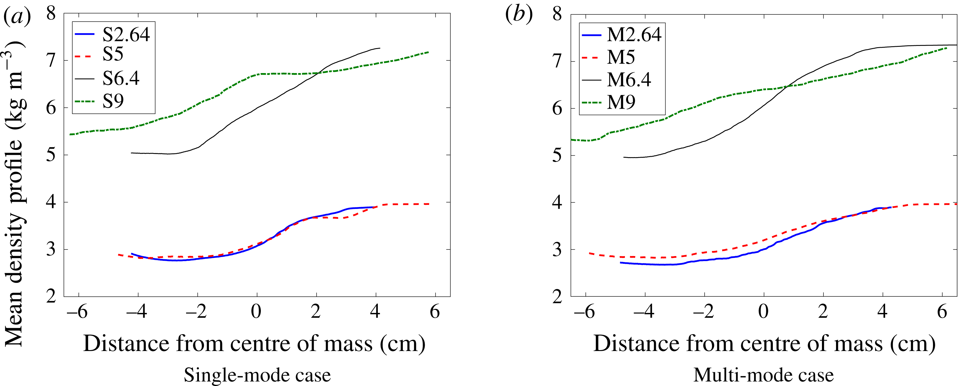
We will now probe the state of the flow by analyzing quantitative concentration fields (correction method described in § 2). Values of density calculated from 1D gas dynamics can be applied to the known values of concentration. From the density fields we can extract statistics that describe the state of mixing and begin to understand the flow field evolution.
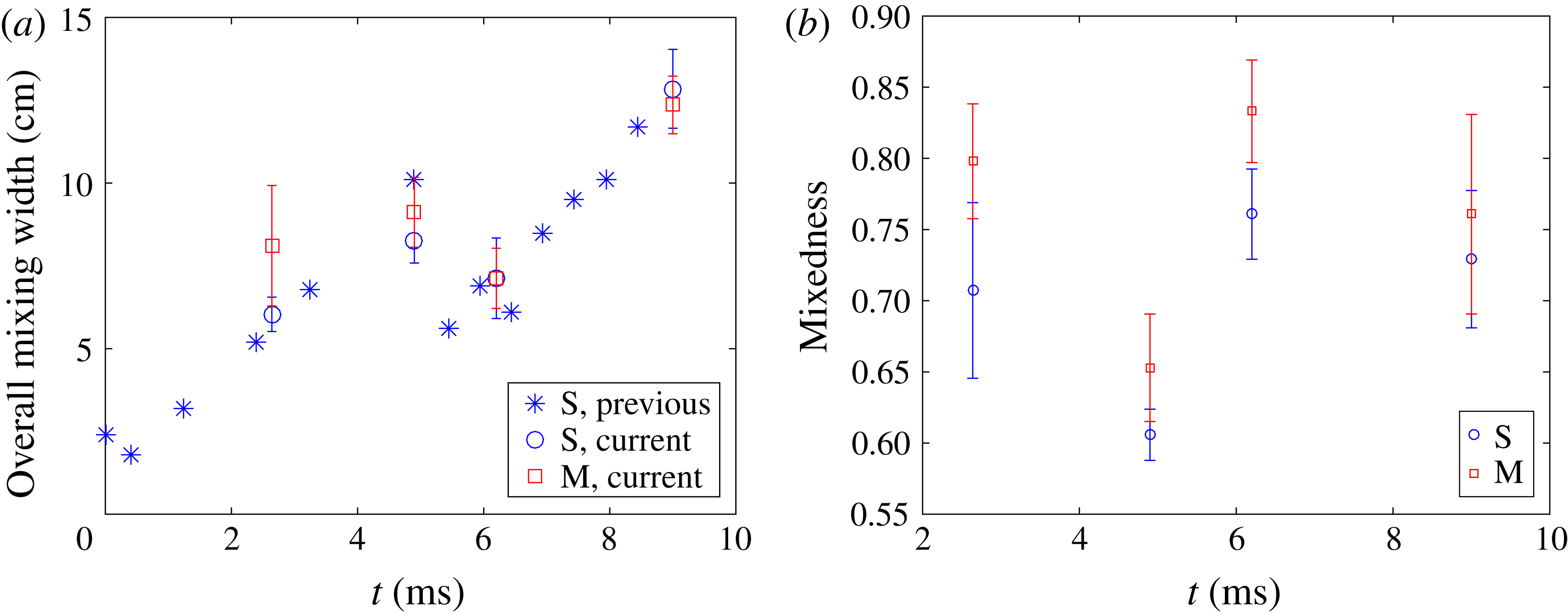
The total width of the mixing region is measured as the distance in the direction of shock propagation between 5 % and 95 % values of the concentration profile (averaged in the direction normal to shock propagation). Figure 6(a) shows the mixed width versus time. The error bars represent plus or minus one standard deviation. The data points without error bars are from a previous study (Reilly Reference Reilly2015), with the same conditions as the single-mode case S presented here, but with only PLIF measurements. The data from the current study is consistent with the previous data as expected, but the multi-mode case displays a slightly larger mixed width at 2.64 ms (note that error bars overlap). The larger mixed width could be due to the inflow of gases slightly above and below the interface, as detailed in § 2, combined with the increased thickness of the mixing layer which is superposed on the inclined interface. The growth of the interface follows a fairly linear trend at the earliest times, as expected for an amplitude-to-wavelength ratio of the inclined perturbation
 $\unicode[STIX]{x1D6FC}=0.088$
, and maintains a trend which is fairly close to linear even until reshock. The linear growth corresponds to the strong penetration seen in the density fields. The overall growth rate of the mixing layer calculated from experiments can be compared to analytical results. The growth rate calculated from experiments is approximately
 $17.2~\text{m}~\text{s}^{-1}$
just after shock passage (initial growth rate is very similar for both cases), for which the linear theory of Richtmyer predicts a growth rate of
 $16.9~\text{m}~\text{s}^{-1}$
(Richtmyer Reference Richtmyer1960). Using the model of Weber, Cook & Bonazza (Reference Weber, Cook and Bonazza2013) to extract the growth rate by modeling vorticity deposition and applying the Biot-Savart law yields a growth rate of
 $17.3~\text{m}~\text{s}^{-1}$
. As secondary instabilities begin to have larger effects, a change in growth rate from linear to non-linear is expected as the penetrating mass spreads through the mixing region more rapidly and homogeneously. Although a strongly nonlinear trend is not obvious, it is apparent that secondary instabilities play a role in the mixing process; we see significant spreading of mass throughout the mixing region in the multi-mode case before and after reshock. Additionally, the post-reshock, single-mode case appears to break up due to secondary instabilities, although the linear perturbation at the largest scale is somewhat separated from the scales at which this mixing is occurring.
(a) Total mixing width at different times for both single-mode (case 1) and multi-mode (case 2), and (b) total mixedness at different times for both single-mode (S) and multi-mode (M) cases.

Mixedness profiles are a measure of how well-entrained fluid is molecularly mixed. If none of the entrained fluid is mixed molecularly (immiscible case) the mixedness is zero, but if all the entrained fluid is molecularly mixed (a pure substance, locally homogeneous) then mixedness is one. The mixedness was calculated using
 $\unicode[STIX]{x1D703}=\overline{\unicode[STIX]{x1D709}_{1}\unicode[STIX]{x1D709}_{2}}/\overline{\unicode[STIX]{x1D709}_{1}}\times \overline{\unicode[STIX]{x1D709}_{2}}$
, where
 $\unicode[STIX]{x1D709}$
represents mole fraction and subscripts 1 and 2 refers to light and heavy gases.
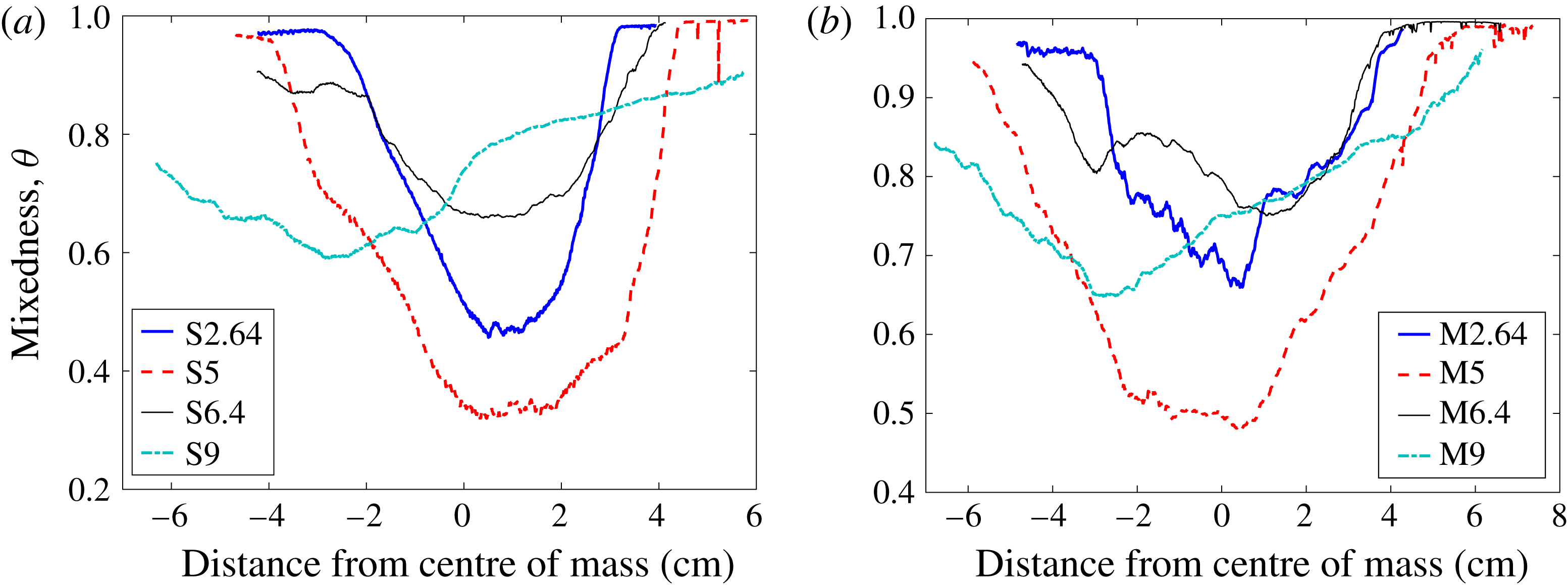
Mixedness can be calculated by averaging over the entire mixing region, as shown in a temporal progression in figure 6(b). The time plot shows that from 2.64 ms to 5 ms the penetration of additional fluid as the interface stretches decreases mixedness due to gradient intensification. Case M shows higher mixedness at times before and just after reshock. After reshock, both cases undergo an increase in mixedness because the mixed material is confined to a smaller region during the inversion. From 6.4 ms to 9 ms the mixedness decreases again due to intensification of the gradients as the interface grows again. Although the mixedness is higher at all times for the multi-mode case, at 9 ms it is the closest between the cases. As the interface stretches, which causes additional entrainment but also increased turbulent mixing, the mixedness remains close to 0.8. Similar to the observations of Schilling et al. (Reference Schilling, Latini and Don2007), Lombardini, Pullin & Meiron (Reference Lombardini, Pullin and Meiron2012) and Tritschler et al. (Reference Tritschler, Olson, Lele, Hickel, Hu and Adams2014) the mixedness approches 0.85 asymptotically, as increased mass is injected into the mixing region and entrained fluid continues to become homogenized by turbulent mixing. It appears that the interface is approaching this point; however, given the extent of inhomogeneity (which remains throughout the mixing region at 9 ms), it is likely that the interface is still approaching the asymptotic state. Moreover, observation of figure 7 gives insight into the how well-mixed fluid is in different regions. Mixing in the bubble region (heavy gas side) is enhanced in the multi-mode case before reshock, while the bubble region of the single-mode case remains sharper before reshock. The effect of the rollup manifests itself in case S, at 5 ms, as a slight bump in the mixedness followed by a sharp upturn to one as as it approaches the pure nitrogen region. The multi-mode case is less mixed in the bubble region at 9 ms, which is evidence of continued turbulence development at smaller scales.
Temporal evolution of mixedness for both (a) single-mode (S) and (b) multi-mode (M).

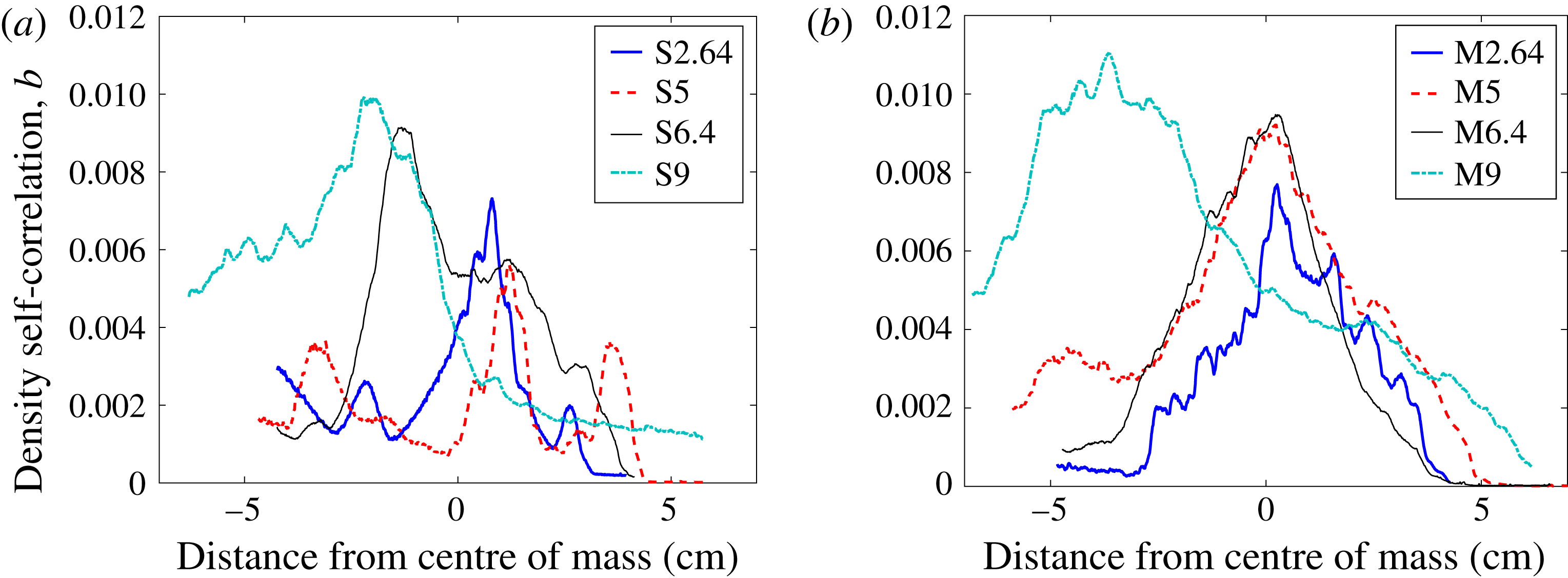
The autocorrelation of density fluctuations with specific volume fluctuations, also known as the density self-correlation (DSC) or the
 $b$
parameter as introduced by Besnard et al. (Reference Besnard, Harlow, Rauenzahn and Zemach1992) in the Besnard, Harlow, and Rauenzahn, or BHR model, helps describe instantaneous mixing occurring in the flow:
 $$\begin{eqnarray}b=-\langle \unicode[STIX]{x1D70C}^{\prime }\unicode[STIX]{x1D708}^{\prime }\rangle ,\quad \unicode[STIX]{x1D708}^{\prime }=(1/\unicode[STIX]{x1D70C})^{\prime }.\end{eqnarray}$$
The averaging in (4.1) has typically been performed in two different ways by the RMI community: spanwise averaging, when there are not enough realizations to form an ensemble, and true ensemble averaging when there are enough realizations. The effect of averaging method on the value of
 $b$
was demonstrated by Balakumar et al. (Reference Balakumar, Orlicz, Ristorcelli, Balasubramanian, Prestridge and Tomkins2012). The DSC, averaged over the spanwise direction, is zero for pure fluids, including homogeneous mixtures, where there is no spatial variance in the density. Thus, the spanwise averaging method describes the level of inhomogeneity in the spanwise direction. If averaged over an ensemble, the DSC is zero where there are no fluctuations from the ensemble. This averaging method produces values for
 $b$
which correspond to the density fluctuation intensity, different information than mixedness provides. Livescu & Ristorcelli (Reference Livescu and Ristorcelli2008) shows the relationship between mixedness and the DSC, and if both are calculated from spanwise averaging they both describe homogeneity (inhomogeneity) in the flow. In the present work, ensemble averaging was used to produce a DSC field which was then averaged in the spanwise direction to obtain profiles along the streamwise direction. Because of the coupling between the density and velocity fields, density fluctuations are selected to the flux of mass (the velocity of the mass flux will be described in detail later) which drives the production of Reynolds stress in the BHR model. The production term of the Reynolds stress from the BHR model (Schwarzkopf et al.
Reference Schwarzkopf, Livescu, Baltzer, Gore and Ristorcelli2016) is
 $$\begin{eqnarray}[a_{i}\overline{P}_{,j}+a_{j}\overline{P}_{,i}]-\overline{\unicode[STIX]{x1D70C}}[\widetilde{R}_{ik}\widetilde{u}_{j,k}+\widetilde{R}_{jk}\widetilde{u}_{i,k}]\end{eqnarray}$$
where
 $a$
is the mass flux.
According to figure 8, the profiles of the DSC are similar at 2.64 ms because the interface has just been compressed by the incident shock. This compression confines the area over which the density can fluctuate while the interface stretching is sharpening the gradients. However, the mixing is slightly higher in the multi-mode case. At 5 ms the profiles are the most different, as the single-mode case shows localized peaks in mixing at shear-driven roll-ups, whereas the multi-mode case shows mixing throughout the mixing layer due to increased mode merging effects. Both cases show similarly high levels of mixing at 6.4 ms due to the recent forcing of the reshock wave. However, at 9 ms, the DSC is higher for case M in the spike tip and bubble regions, which is evidence that turbulent mixing mechanisms in those regions persist even after the forcing of reshock has ceased. The mixing intensity at 9 ms after reshock is commensurate with the asymptotic theory of mixedness in that as more fluid is injected into the mixing region, which is growing nonlinearly, density fluctuations act in synergy with strong velocity fluctuations, which describes the motivation for (4.2).
Temporal evolution of the combined density self-correlation for both (a) single-mode (S) and (b) multi-mode (M) cases.

To conclude analysis of the density fields, and preface subsequent discussion on the velocity fields, the density gradients are analyzed in conjunction with vorticity. The PLIF resolution is not sufficient to show the exact scalar dissipation rate with
 $Sc\approx 1$
, the Batchelor scale,
 $\unicode[STIX]{x1D706}_{b}\approx \unicode[STIX]{x1D706}_{k}$
(
 $\text{resolution}\approx 7\unicode[STIX]{x1D706}_{b}$
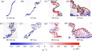
); however, the dissipation rate filtered by the resolution scale is provided in appendix C. An alternative method of visualizing density gradients is a simulated schlieren technique (Quirk & Karni Reference Quirk and Karni1996) which is shown in figure 10 with the vorticity overlaid. This result from simultaneous measurements provides a description of how well the small-scale features of the flow (scalar and velocity gradients) are connected. The simulated schlieren field is derived from the density field by
 $$\begin{eqnarray}\unicode[STIX]{x1D6F7}(x,y,t)=\exp \bigg\{-\unicode[STIX]{x1D705}\frac{|\unicode[STIX]{x0394}\unicode[STIX]{x1D70C}|}{|\unicode[STIX]{x0394}\unicode[STIX]{x1D70C}|_{max}}\bigg\},\quad \unicode[STIX]{x1D705}=\left\{\begin{array}{@{}ll@{}}100\quad & \unicode[STIX]{x1D709}<0.75\\ 20\quad & \unicode[STIX]{x1D709}>0.75\end{array}\right.,\end{eqnarray}$$
where
 $\unicode[STIX]{x1D709}$
is mole fraction. Sharper gradients appear darker in the images. Most of the mixing region in case S has sharper gradients at each experimental time. The gradients appear sharper towards the spike side (light gas side, left) of the interface at all times as the pure heavy gas is injected into the light gas and the resultant shearing strips off mass as it mixes. The multi-mode case appears to break down to smaller scales much more quickly than the single-mode case, but both appear to have become much more disorganized at 9 ms. The vorticity is discussed in further detail in the subsequent section.
4.2 Analysis of velocity field
In this section, the acquired velocity fields are analyzed and discussed through the use of vorticity fields (pre- and post-reshock) and the effect of the velocity-averaging method on Reynolds stress profiles is discussed. Probability density functions (PDFs) of velocity fluctuations (Orlicz et al.
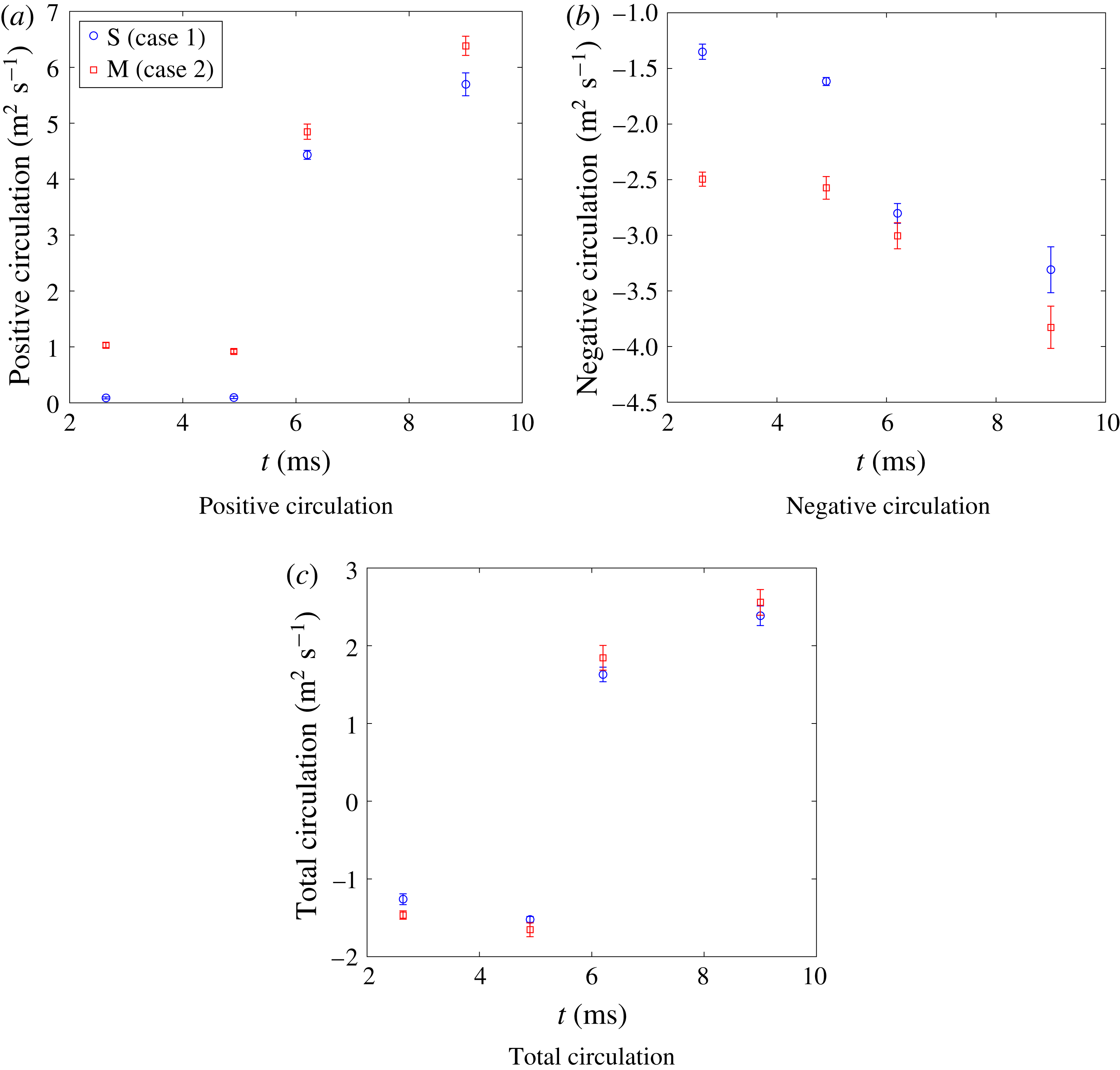
Reference Orlicz, Balasubramanian, Vorobieff and Prestridge2015), and the positive, negative and total circulation are explained in appendix C. In order to reliably perform velocity field analysis, the velocity fluctuations must be calculated correctly, from spanwise or ensemble averaging. To calculate velocity fluctuations using spanwise averaging, the bulk velocity
 $u_{b,i}$
was defined as the streamwise and spanwise spatial average of the
 $i$
th component of the velocity. The relative velocity was then defined as the difference between the instantaneous and bulk velocities,
 $$\begin{eqnarray}\displaystyle & \displaystyle u_{b,i}(en)=\langle u_{i}(x,y,en)\rangle _{x,y} & \displaystyle\end{eqnarray}$$
 $$\begin{eqnarray}\displaystyle & \displaystyle u_{r,i}(x,y,en)=u_{i}(x,y,en)-u_{b,i}(en). & \displaystyle\end{eqnarray}$$
Next, the relative velocity was spatially averaged over the spanwise or
 $y$
-direction. Then the velocity fluctuation,
 $u^{\prime }$
, was defined as the relative velocity minus the spanwise-averaged velocity,
 $$\begin{eqnarray}\displaystyle & \displaystyle \overline{u_{r,i}}(x,en)=\langle u_{r,i}(x,y,en)\rangle _{y} & \displaystyle\end{eqnarray}$$
 $$\begin{eqnarray}\displaystyle & \displaystyle u_{i}^{\prime }(x,y,en)=u_{r,i}(x,y,en)-\overline{u_{r,i}}(x,en). & \displaystyle\end{eqnarray}$$
Comparison of Favre-averaged Reynolds stress components in the multi-mode case at 9 ms based on two methods of velocity fluctuation calculation: (a) spatial versus (b) ensemble averaging.

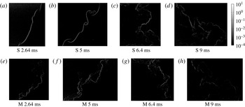
Vorticity evolution overlaid on simulated schlieren images for both cases. S refers to single-mode case and M refers to multi-mode case.

Velocity fluctuations found using ensemble averaging were obtained by taking the difference between the instantaneous velocity and an ensemble average. Equations (4.8) and (4.9) show the ensemble average, which is defined as the velocity at each
 $x,y$
location averaged over all realizations at each experimental time:
 $$\begin{eqnarray}\displaystyle & \displaystyle \overline{u_{i}}(x,y)=\langle u_{i}(x,y,en)\rangle _{en} & \displaystyle\end{eqnarray}$$
 $$\begin{eqnarray}\displaystyle & \displaystyle u_{i}^{\prime }(x,y,en)=u_{i}(x,y,en)-\overline{u_{i}}(x,y). & \displaystyle\end{eqnarray}$$
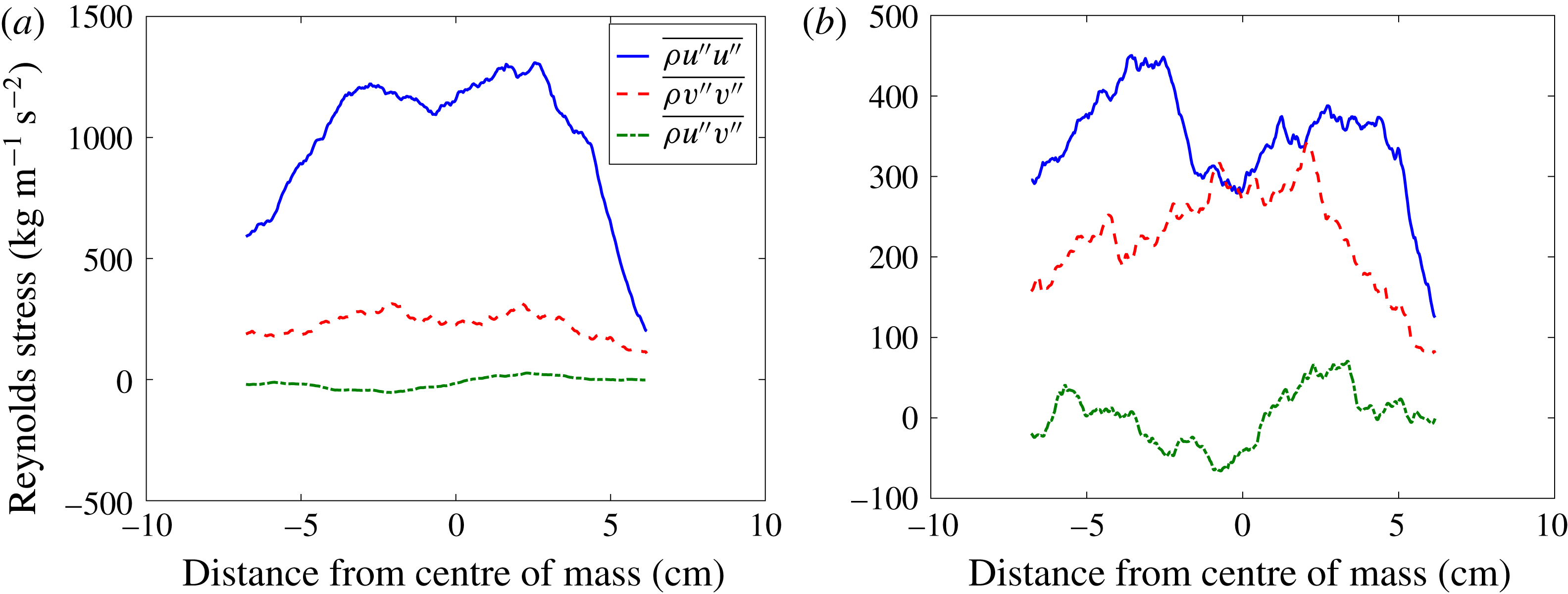
The two methods yield different results. To highlight the effect of ensemble averaging versus the use of traditional spanwise averaging, Favre-averaged Reynolds stresses for case M at 9 ms (late time, post-reshock) are shown in figure 9. For the Favre-averaged Reynolds stress, velocity fluctuation components come from mass-weighted average quantities:
 $\tilde{u_{i}}=\overline{\unicode[STIX]{x1D70C}u_{i}}/\overline{\unicode[STIX]{x1D70C}}$
. Figure 9 shows that the most significant difference between the two methods is the magnitude of the
 $u^{\prime \prime }u^{\prime \prime }$
term, which is significantly higher when using spanwise averaging, due to the large fluctuations in the streamwise velocity across the interface. The
 $v^{\prime \prime }v^{\prime \prime }$
and
 $u^{\prime \prime }v^{\prime \prime }$
terms are similar in magnitude but show more variation across the interface in the ensemble averaged case. We expect this variation would decrease as more experiments are executed. In a statistically repeatable, homogeneous turbulent flow field it would be expected that the ensemble and spatial averages would yield the same result. Comparatively, in our flow field the spanwise velocity is relatively insensitive to the averaging method, suggesting it is homogeneous in the spanwise direction. However, the large difference in the streamwise direction highlights the need for ensemble averaging due to the inhomogeneity of the streamwise velocity across the interface. Consequently, velocity statistics were calculated using ensemble averaging.
Resolving the vorticity field and flow circulation are two key aspects of a velocity field analysis. Using the PIV methods outlined earlier, the velocity fields were resolved using TSI INSIGHT 4G™ in order to provide a quantitative analysis of the flow field. Any holes in the velocity fluctuation field were filled via interpolation using nearby values. The field was subsequently filtered using a median filter with a bin of 11-by-11 vectors in order to smooth spurious noise induced by small gradients in the fields and allow for a more accurate analysis. The two methods that have been used to compute vorticity are explained in appendix C.
The evolution of the vorticity field is shown in figure 10, where red and blue represents positive and negative vorticity, respectively. Due to the misalignment of the pressure and density gradients, the baroclinic term results in vorticity deposition across the flow field, which in turn results in mixing and deformation of the interface. For the single-mode case, shown starting with figure 10(a), the incident shock wave passing from light to heavy gas creates strong negative vorticity across the interface. The magnitude of the vorticity immediately after incident shock compares well with the analytical model of Weber et al. (Reference Weber, Cook and Bonazza2013), which gives approximately
 $0.9\times 10^{4}~\text{s}^{-1}$
. At 5 ms after incident shock, the vorticity deposited on the interface has caused the initial perturbations to grow in amplitude and form larger vortical structures, as seen in figure 10(b). As the amplitude of the perturbation is larger than the IC and the density gradients are enhanced, it is expected that a larger amount of vorticity will be deposited as the reshock wave passes back from the heavy to light gas regions, leading to much higher levels of vorticity (Weber et al.
Reference Weber, Haehn, Oakley, Rothamer and Bonazza2012). This can be seen in figure 10(c), where as the reshock wave passes through the interface, it deposits such a large amount of vorticity that the majority of the field becomes positive. This reversal of the vorticity field is a result of the application of additional opposite-signed (now positive) baroclinic torque, and the interface itself begins to rotate in the opposite direction immediately after reshock. Furthermore, small pockets of negative vorticity are preserved even after reshock. The presence of positive and negative vorticities after reshock, seen in figure 10(d), is a result of vorticity deposition on an interface with a much less unidirectional gradient. It is also apparent that, due to the more mixed state of the reshock initial condition (5 ms), there is a larger area of the flow over which vorticity is deposited.
For the multi-mode case, shown as a progression starting from figure 10(e), the general physics is similar but key differences should be highlighted. In figure 10(e), immediately following the incident shock wave, the complex nature of the multi-mode interface has already resulted in the deposition of positive vorticity even before reshock. In figure 10(f), the vorticity has grown again, feeding the growth of the perturbations that serve as the initial conditions for the multi-mode reshock case. Figure 10(g) shows the vorticity field immediately prior to reshock and displays the anticipated deposition of positive vorticity due to the application of baroclinic torque. As expected, the deposition of vorticity in the multi-mode case results in higher-amplitude positive vorticity post-reshock than in the single-mode case, due to the presence of positive vorticity pre-reshock. However, this figure displays a notable difference between the two cases, as although the amount of vorticity deposition is equivalent, its distribution is markedly different. In the single-mode case, the vorticity deposition occurs along the interface, as it closely follows its shape. Whereas in the multi-mode case the distribution of vorticity deposited is broader and more diffuse. Lastly, it can again be seen from figure 10(h) that by late time the vorticity becomes more widely deposited throughout the flow field, its amplitude grows, and the level of mixing increases.
4.3 Analysis of simultaneous velocity and density field statistics
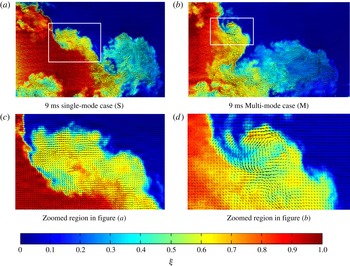
Figure 11 shows velocity vector fields which have been registered to density fields as discussed in § 2. This visualization shows the connection between the velocity field and the density field, and highlights that there is a velocity gradient across the density gradients, especially at the edge of the mixing layer where the density gradient is strong. However, a more chaotic state is present in the bubble region, which is generally more mixed, but still contains a level of local inhomogeneity.
The alignment of vorticity with concentration gradients is just one example of the utility gained by registering the simultaneous density and velocity fields. Density-velocity statistics are critical to validation of turbulence models for variable-density flows and give insight into the physics of multi-component mixing in the developing RMI flow.
Registered velocity and concentration fields for 9 ms multi-mode and single-mode inclined cases. (a,b) Include
 $1/4$
of the velocity field resolution and indicate the regions to be zoomed in (c,d), which show
 $1/2$
of the velocity field resolution for clarity.

The mass flux due to turbulent fluctuations found by correlating the density and velocity fluctuations, is
 $a_{i}=\overline{\unicode[STIX]{x1D70C}^{\prime }u_{i}^{\prime }}/\overline{\unicode[STIX]{x1D70C}}$
. The overbar represents an ensemble average which yields a field of values. To obtain a profile, the fields are averaged in the spanwise direction.
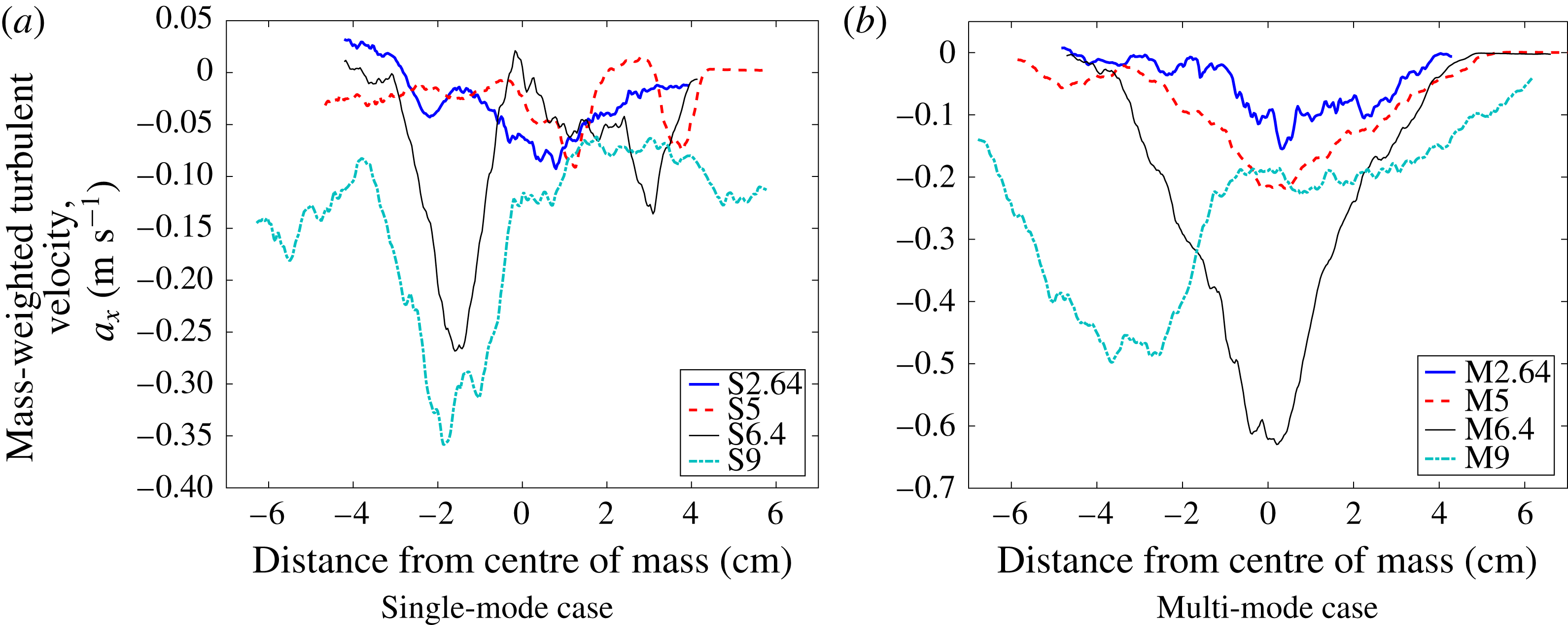
The streamwise velocity mass flux is shown in figure 12. Based on the choice of axes, a negative value denotes that, on average, positive fluctuations in density correspond to a velocity fluctuation in the streamwise-direction toward the region of pure light gas while negative fluctuations in density correspond to a velocity fluctuation in the opposite direction. This leads to turbulent interpenetration.
Temporal evolution of the combined turbulent mass flux in the streamwise direction of the velocity fluctuations. Single-mode (S) and multi-mode (M) cases.

It is obvious that at all times case M has more fluctuating mass flux across the majority of the mixing layer. At the earliest time, 2.64 ms, the two cases appear very similar in shape, but with slightly more flux in the multi-mode case. At 5 ms, two small negative peaks can be seen in the single-mode case where shear-driven rollups cause increased fluctuations, while the multi-mode case has a maximum near the centre of mass where POD analysis of the initial condition suggests there is significant modal content. Reshock amplifies the flux in both cases as more energy is delivered to the mixing region. At 6.4 ms, the single-mode case shows peaks at the edges of the mixing region where there is intense penetration. The multi-mode case shows a similar level of flux near the edges, but a maximum near the centre of mass. At the latest time (9 ms) the bubble region (the right side of the image) is becoming more homogenized, and therefore has less mass flux than the spike region, where a sharper contrast in density yields more intense flux of mass. Similar to 6.4 ms, the multi-mode case has greater mass flux over almost the entire domain, reinforcing the assumption that the multi-mode case is in a state of more active turbulent development.
4.4 Reynolds stresses and anisotropy
In this section we examine the anisotropy of the flow field through the Reynolds stresses, quantified by the normalized anisotropy tensor:
 $$\begin{eqnarray}\unicode[STIX]{x1D6FD}_{ij}=\frac{\unicode[STIX]{x1D619}_{ij}}{R_{kk}}-\frac{1}{3}\unicode[STIX]{x1D6FF}_{ij},\quad \unicode[STIX]{x1D619}_{ij}=\overline{\unicode[STIX]{x1D70C}{u_{i}}^{\prime \prime }{u_{j}}^{\prime \prime }}/\overline{\unicode[STIX]{x1D70C}}.\end{eqnarray}$$
The components of the tensor are bounded by
 $-1/3$
to
 $2/3$
, where a value of
 $-1/3$
indicates the component has no energy while a value of
 $2/3$
indicates the component contains all of the energy. A value of zero is approached as the Reynolds stresses become equal, indicating an isotropic turbulent energy. For our case, only the streamwise and spanwise components of velocity are available and so we assume that the fluctuations in the out-of-plane direction are equal to those of the spanwise direction. This sets
 $\unicode[STIX]{x1D6FD}_{22}$
equal to
 $\unicode[STIX]{x1D6FD}_{33}$
. This assumption is likely less accurate before reshock, but is a necessary limitation of 2D PIV measurements.
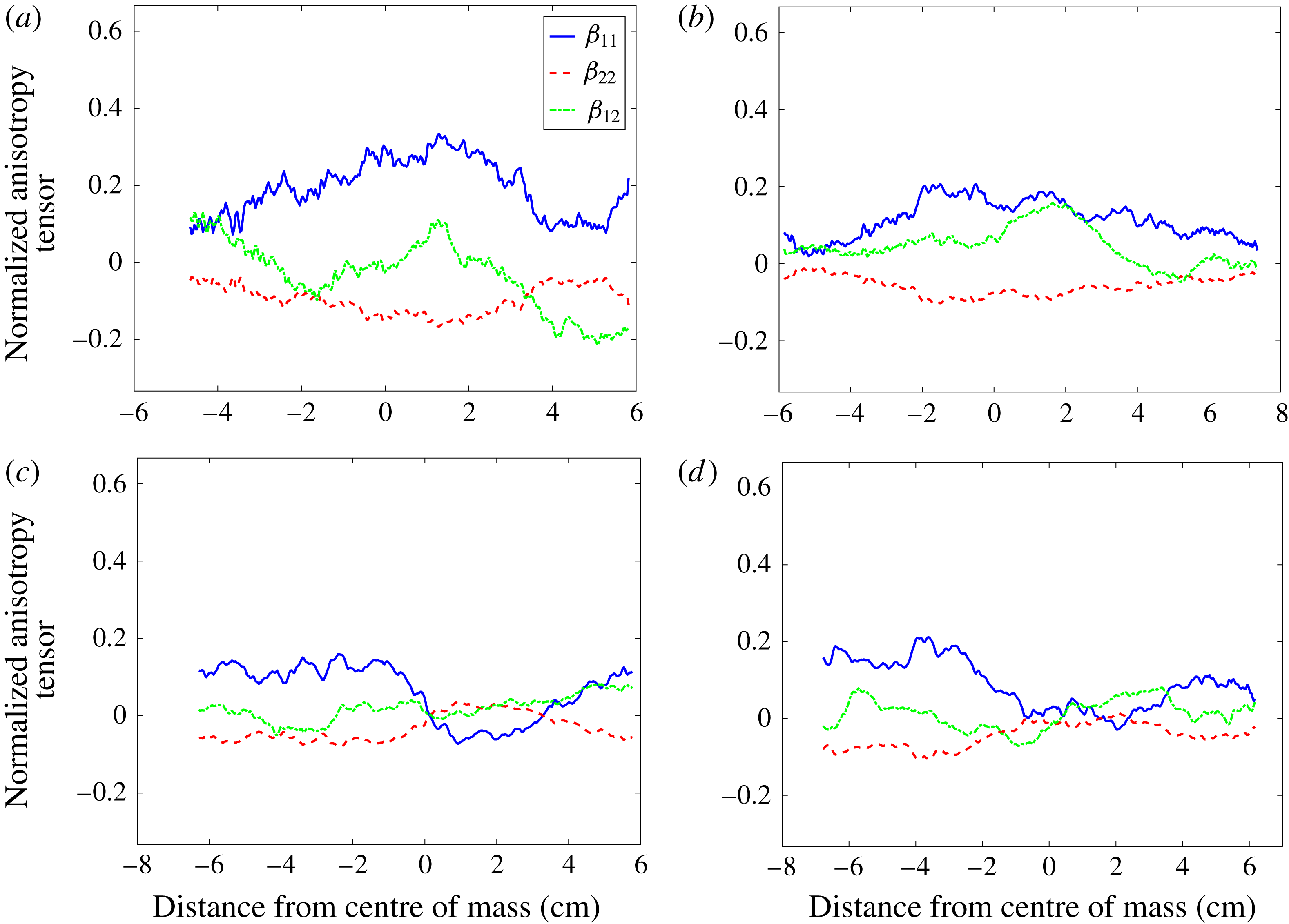
Figure 13 shows the components of the spanwise average of the normalized anisotropy tensor for each case at two times, immediately before reshock (5 ms), and late after reshock (9 ms). From this figure it is evident that the anisotropy decreases after reshock for both cases, with large regions of nearly equal components near the centre of mass in the flow. Before reshock, both cases show a peak in anisotropy near the centre of mass, though the single-mode case shows a higher anisotropy. Both cases at 9 ms show strong non-zero values for the
 $\unicode[STIX]{x1D6FD}_{11}$
and
 $\unicode[STIX]{x1D6FD}_{22}$
components in the upstream flow field, indicating that the former, pre-reshock bubble region now contains the majority of anisotropy. In the downstream region of the post reshock flows we see a much more isotropic region, with the
 $\unicode[STIX]{x1D6FD}_{22}$
term taking a positive value.
The normalized anisotropy tensor components at (a,b) 5 and (c,d) 9 ms for both (a,c) single-mode and (b,d) multi-mode cases.

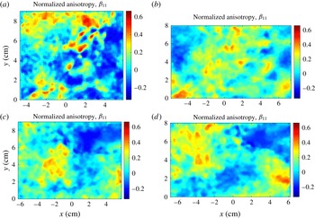
Additional insight into the flow can be gained by examining the spatial distribution of the anisotropy components. Figure 14 shows the spatial distribution of
 $\unicode[STIX]{x1D6FD}_{11}$
. It is noticeable that the anisotropy does not drop to zero away from the interface, due to a small amount of noise which manifests predominantly in the streamwise direction. Although the magnitude of some of the velocity fluctuations away from the interface is small compared to the fluctuations at the interface, the normalization of anisotropy does not typically weight the magnitude of fluctuations because it is classically used in homogeneous flows. Nevertheless, it is customary to present information about inhomogeneous flow in this context while understanding the caveats involved. Before reshock,
 $\unicode[STIX]{x1D6FD}_{11}$
is highest upstream of the interface in the bubble-front region and near the spike tip. The single-mode inclined interface case shows a less well organized field due in part to its less turbulent flow field. After reshock, these regions persist and are transported by the overturning process. The downstream region now contains the high
 $\unicode[STIX]{x1D6FD}_{11}$
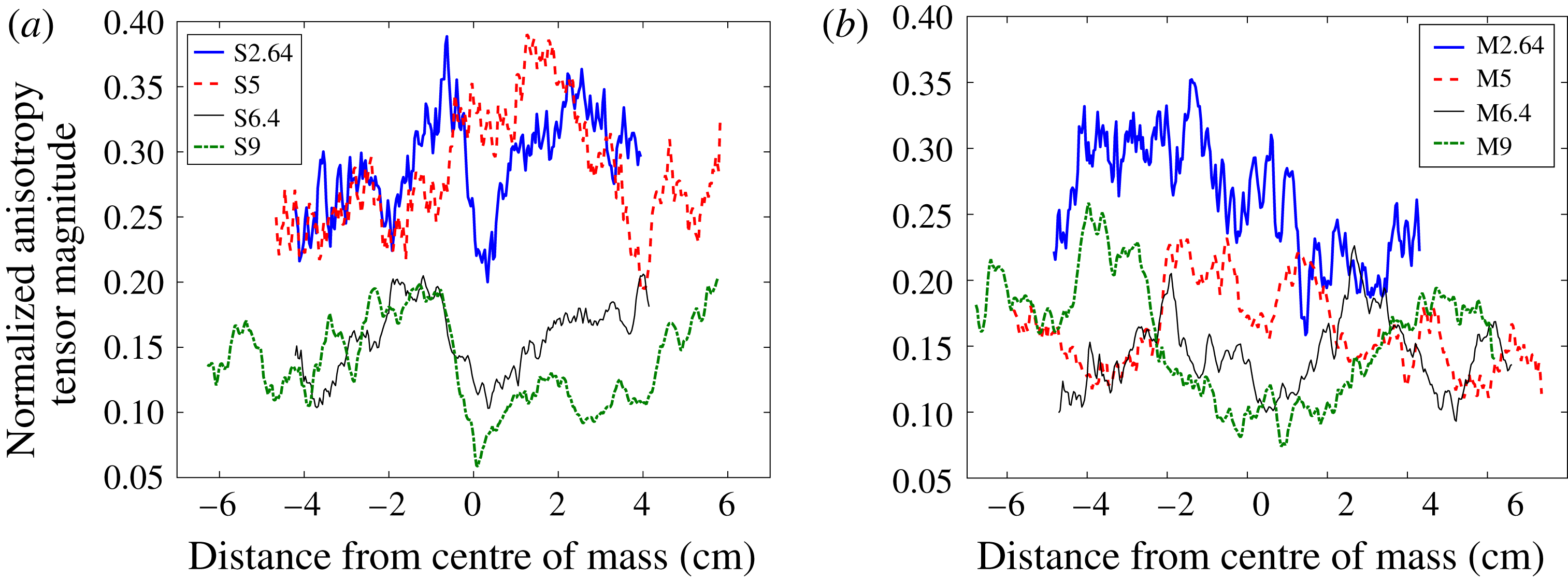
found in the pre-reshock spike while the anisotropy of the pre-reshock bubble front is pushed upstream by the emerging post-reshock spike structure. In order to consider the trend of anisotropy over time, where much lower anisotropy for the multi-mode case before reshock can be seen more clearly, the spanwise average of normalized anisotropy tensor magnitude is shown and explained in appendix C.
 $\unicode[STIX]{x1D6FD}_{11}(x,y)$
for each case at (a,b) 5 ms (before reshock) and (b,d) 9 ms (late time post reshock). (a,c) Single-mode and (b,d) multi-mode cases.

4.4.1 The Boussinesq approximation
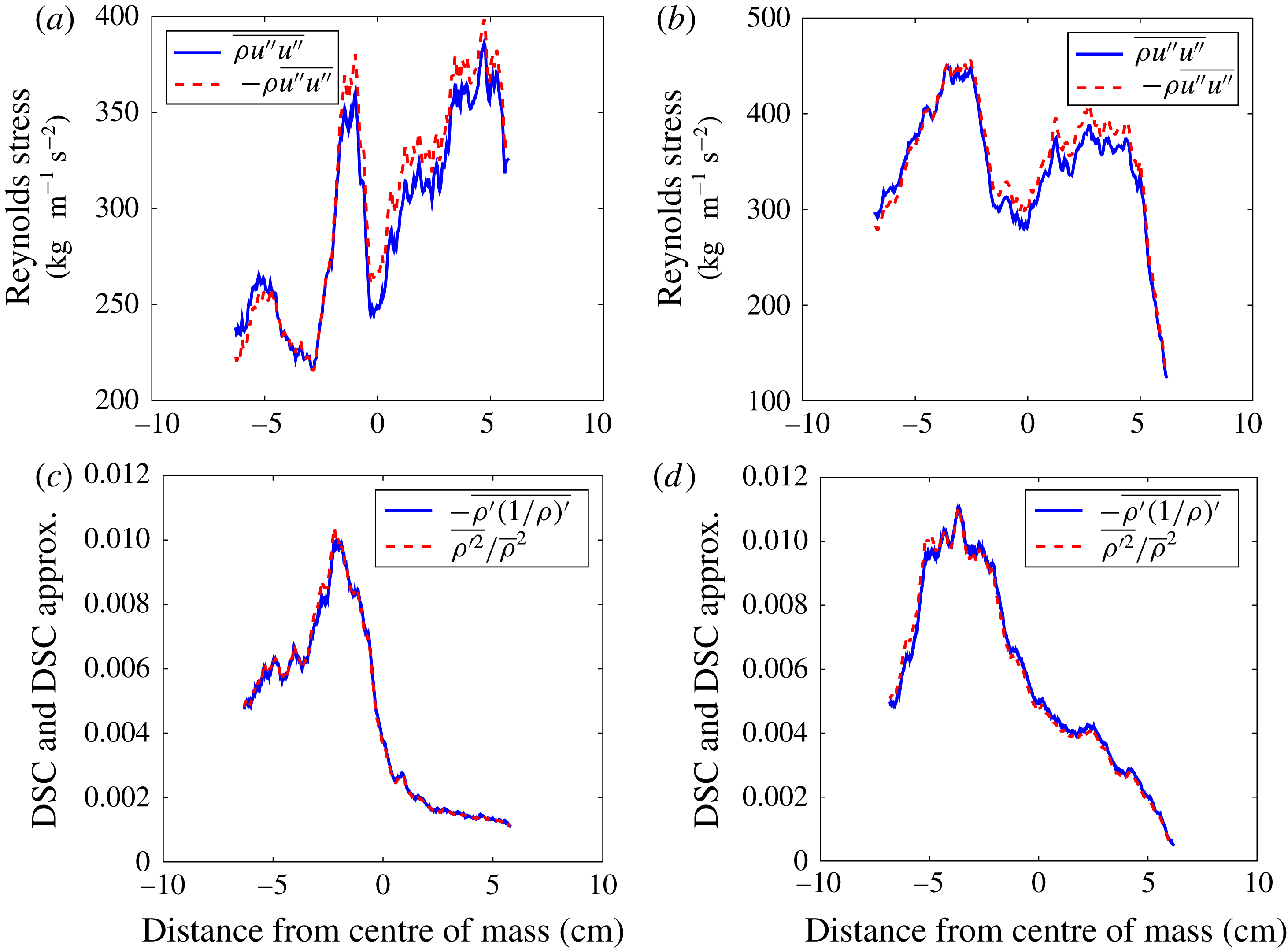
Figure 15 shows a comparison of the Reynolds stress and density self-correlation values compared to approximations which do not account for the variation of the density field at late post-reshock times. Comparing the Favre-averaged Reynolds stress, accounting for density variations, to the Reynolds-averaged Reynolds stress multiplied by the spanwise average density shows a small variation in the Reynolds stress values, within 5 %. The density self-correlation also shows a very similar value to its approximation, again within 5 % of its approximation, as expected as our densities differ by less than a factor of two. The approximation for the DSC used here, the first term of its Taylor expansion (Livescu & Ristorcelli Reference Livescu and Ristorcelli2008), has also been compared to the DSC by Tomkins et al. (Reference Tomkins, Balakumar, Orlicz, Prestridge and Ristorcelli2013), who saw good agreement except at the edge of the mixing region using a fluid layer of
 $SF_{6}$
in air.
Comparison of (a,b) Favre-averaged Reynolds stress to its approximation and (c,d) density self correlation (DSC) to first term of Taylor series expansion of DSC both at 9 ms. (a,c) Single-mode case and (b,d) multi-mode case.

5 Analysis of flow transition
In this section, turbulent length scales derived from the density and velocity fluctuation fields are discussed. Taylor microscales and integral scales are calculated to estimate the inertial range and amount of decadal separation in different velocity and density spectra. Using three different methods, Reynolds numbers are calculated and subsequently used to compute inner viscous and Liepmann–Taylor scales. Finally, transition to turbulence is discussed in regard to its relation to length scales and Reynolds number, and by analyzing different velocity and density spectra.
5.1 Turbulent length scales and Reynolds numbers
The Taylor microscale can be defined using two methods. The first method is based on fitting a quadratic function to the peak and two points, both on the right side of the peak, of the velocity or density fluctuation autocorrelations. The slope of the resulting curvature at
 $f(0)$
is 0 (Pope Reference Pope2000; Ramaprabhu & Andrews Reference Ramaprabhu and Andrews2004). The average of the correlation functions for each field can be defined as
 $$\begin{eqnarray}f(r)=\frac{\langle F(x,y)F(x+r,y)\rangle }{F^{2}},\end{eqnarray}$$
where
 $F$
is density or velocity fluctuation (streamwise or spanwise), and
 $\langle F(x,y)F(x+r,y)\rangle$
is the spatial average (over
 $x$
and
 $y$
) and the ensemble average over all the fields. Correlation functions can also be used to calculate the integral scale by finding the area under the curve of
 $f(r)$
,
 $$\begin{eqnarray}L_{11}=\int f(r,t)\,\text{d}r.\end{eqnarray}$$
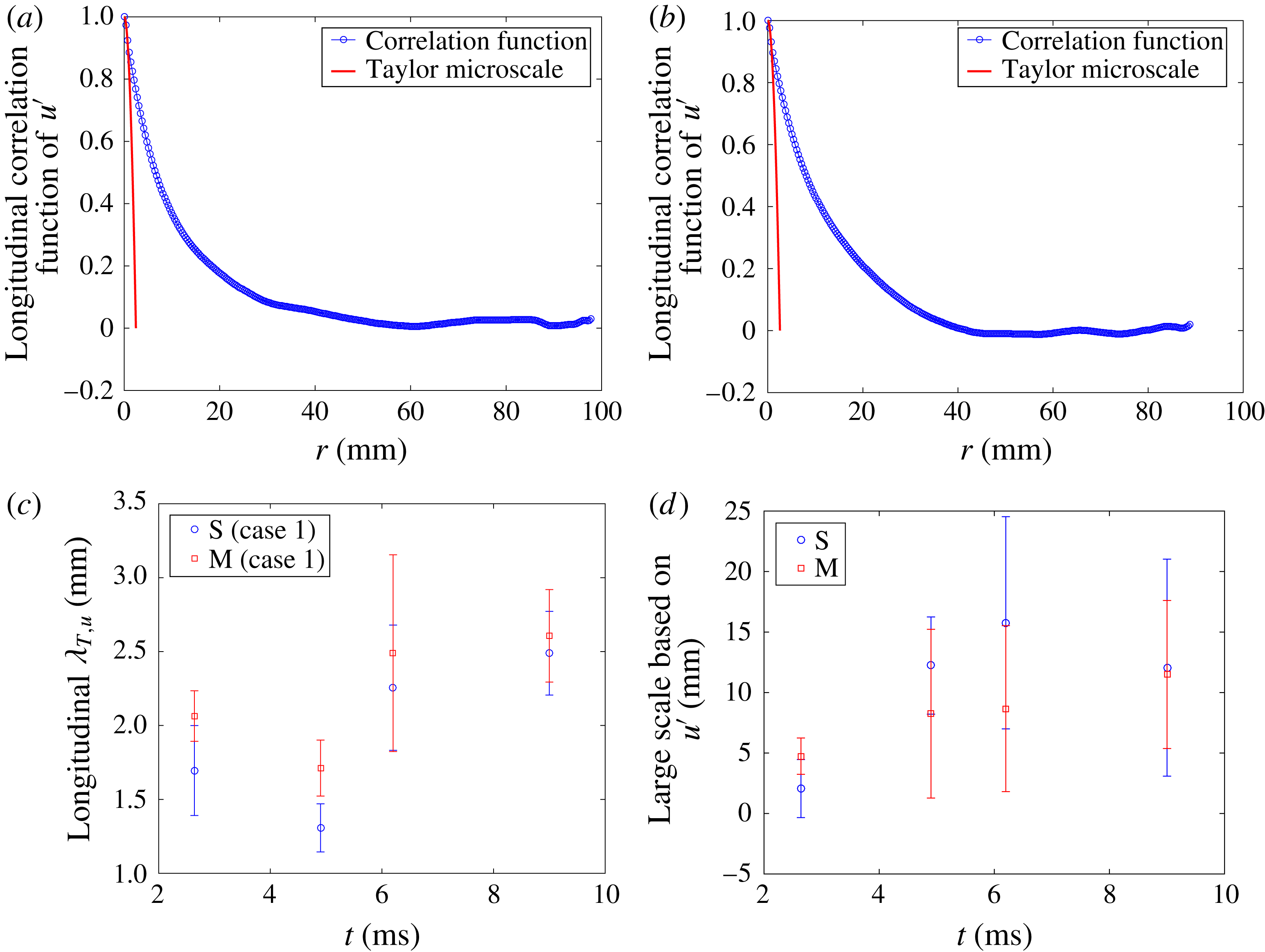
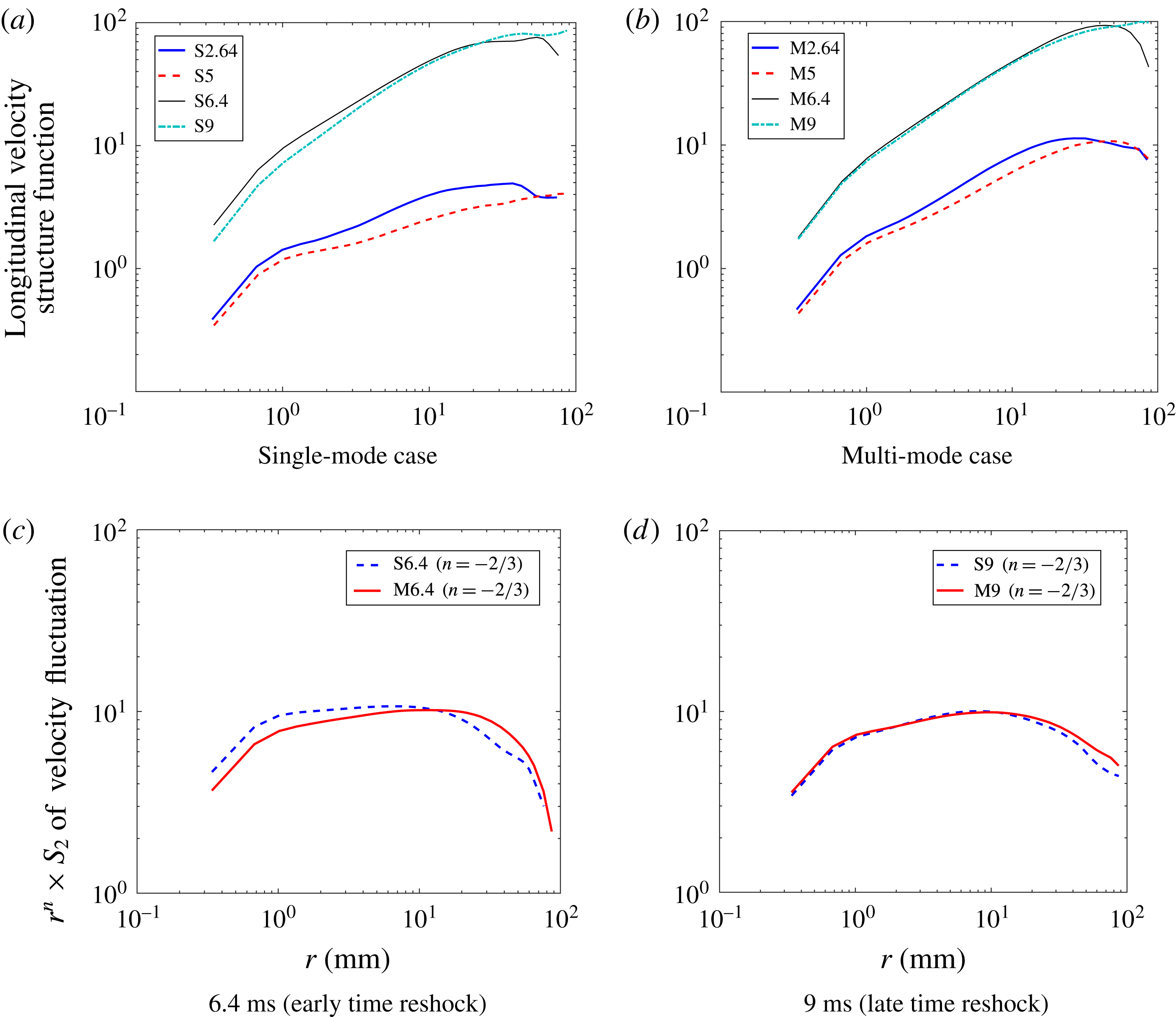
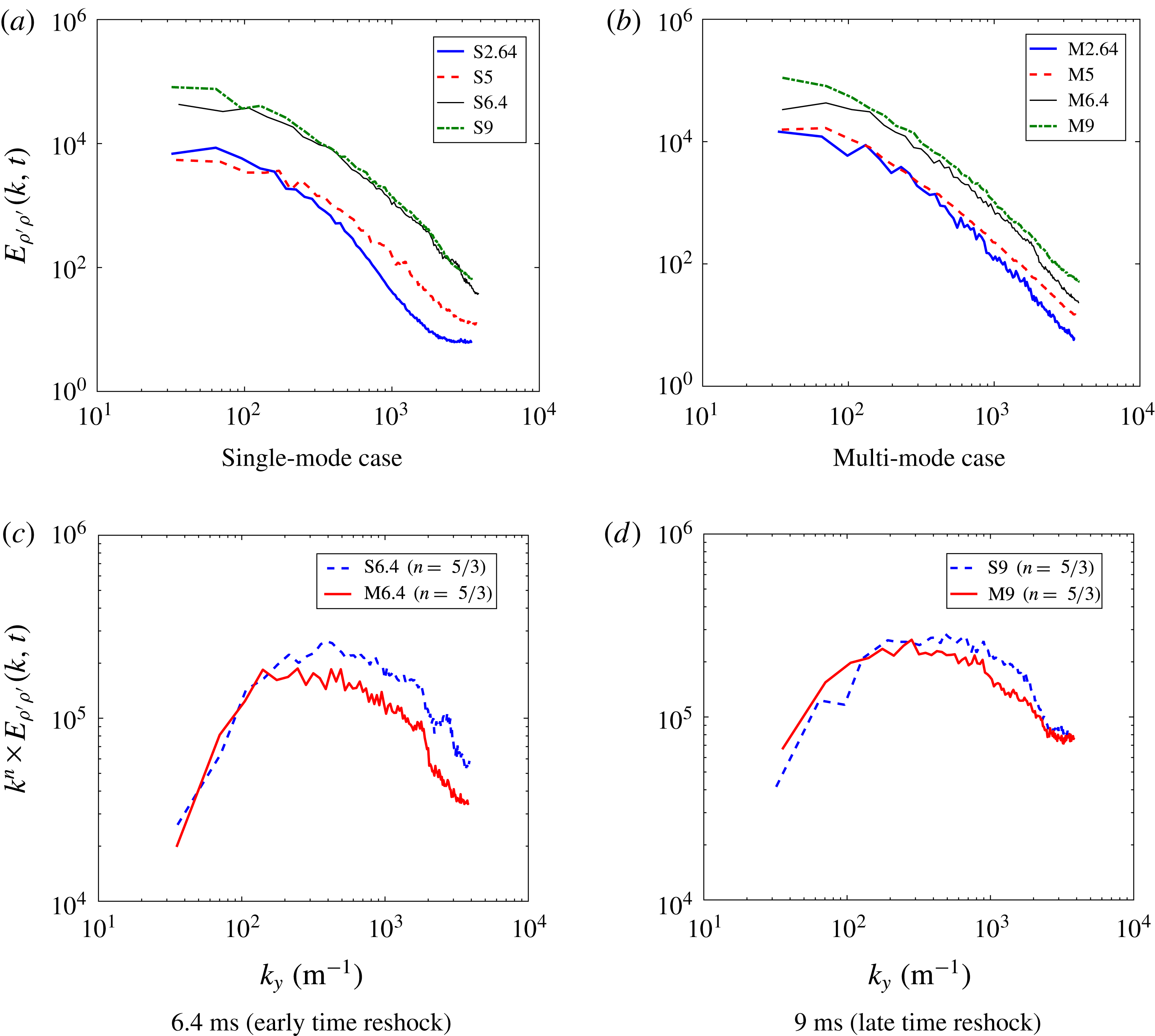
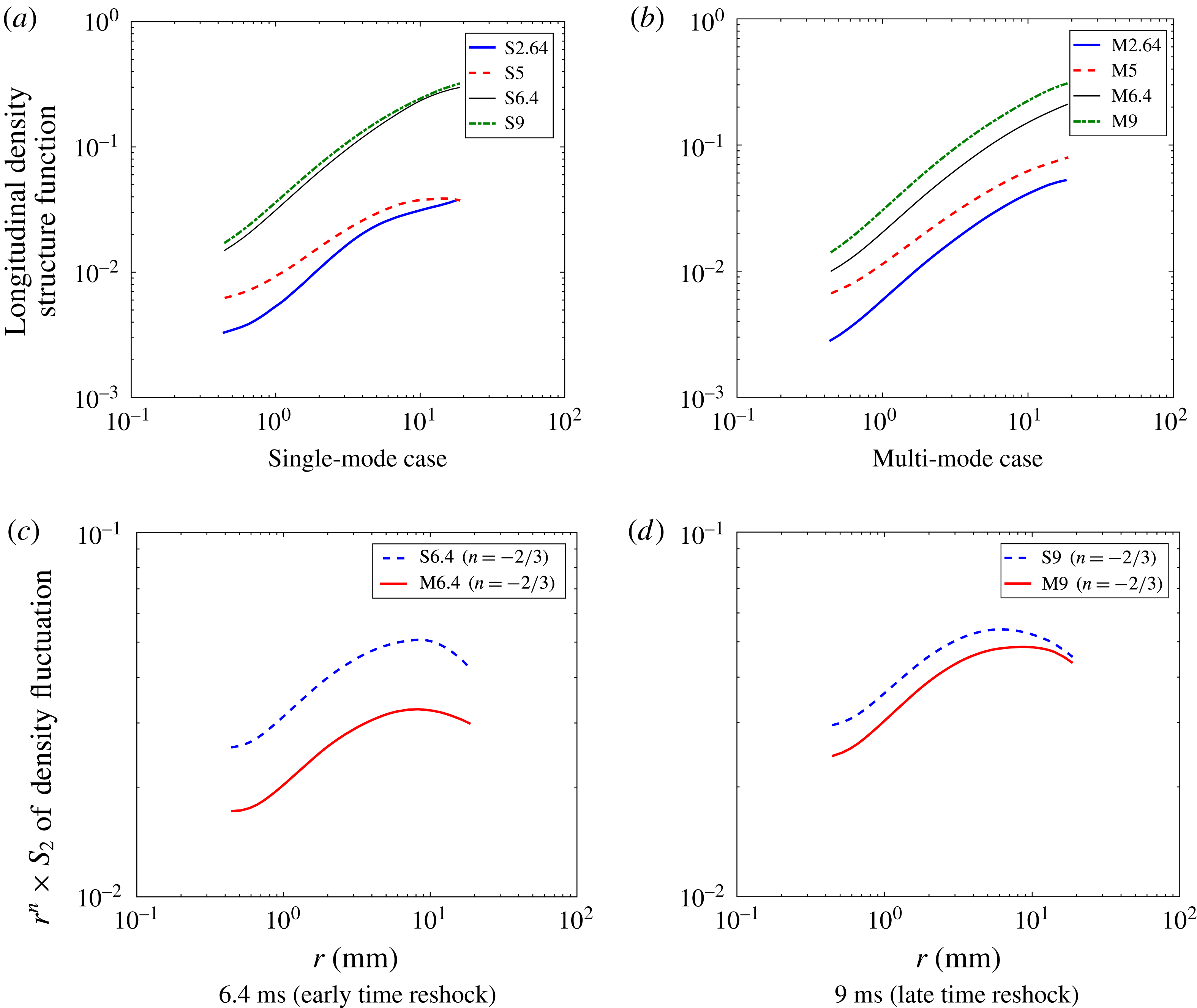
Using correlation functions to calculate Taylor microscales and integral scales is useful for estimating the inertial range in energy spectra. Consider an example using the longitudinal correlation function of streamwise velocity fluctuations at 9 ms, as is shown for the single-mode and multi-mode cases in figures 16(a) and 16(b), respectively. To find the slope of the energy spectra, one must calculate the least-squares fit of the points between the Taylor micro and integral scales in the energy spectra. The error bars in figure 16 represent plus or minus one standard deviation. Inspection of figure 16 suggests that the separation between micro and integral scales, which is also an indication of the inertial range in the energy spectra, will increase after reshock. Furthermore, at 6.4 ms the highest
 $L/\unicode[STIX]{x1D706}=23/2.4\approx 10$
is observed in the single-mode case.
Correlation functions of streamwise velocity fluctuation for both cases at 9 ms (a,b) and the temporal evolution of the corresponding Taylor microscales (c) and integral scales (d) calculated from the correlation functions.

An alternative method for calculating the Taylor microscale is by computing the variance and gradient of the velocity or density fluctuations (Pope Reference Pope2000). Thus the Taylor microscale can be calculated as
 $$\begin{eqnarray}\unicode[STIX]{x1D706}_{T,\unicode[STIX]{x1D702}}=\sqrt{\frac{2\overline{\unicode[STIX]{x1D702}_{i}^{\prime ^{2}}}}{\overline{(\unicode[STIX]{x2202}\unicode[STIX]{x1D702}_{i}^{\prime }/\unicode[STIX]{x2202}x_{i})^{2}}}},\end{eqnarray}$$
where
 $\unicode[STIX]{x1D702}$
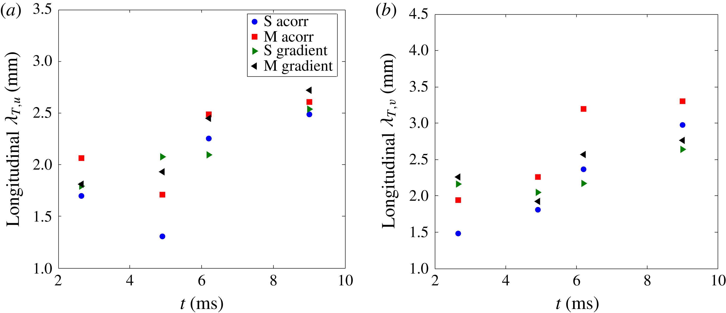
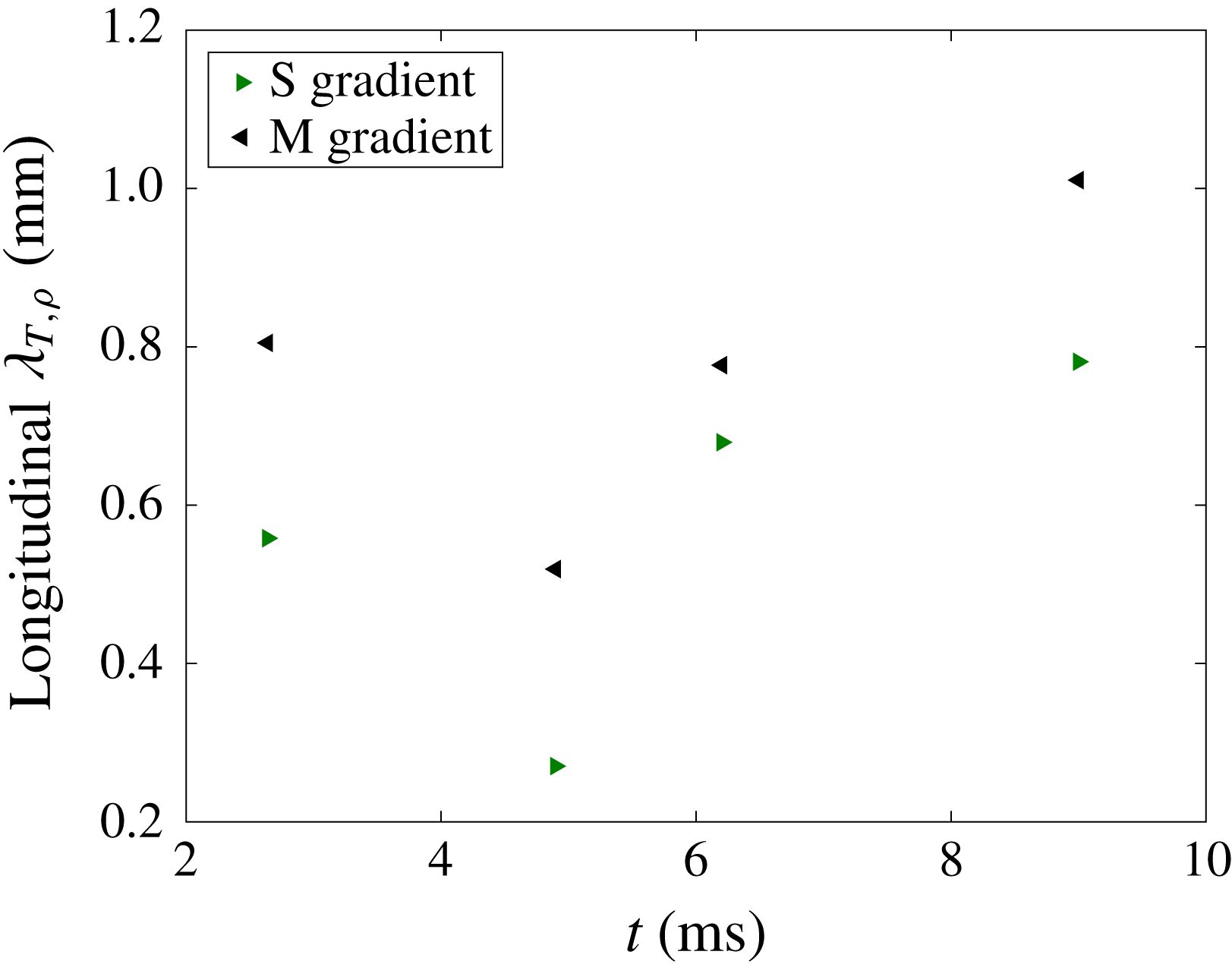
is the velocity or density field. According to figure 17, both methods show similar trends for Taylor microscales given by the velocity fluctuations, as both increase after reshock. Figure 17 also shows that the Taylor microscales from streamwise and spanwise velocity fluctuations are higher in the multi-mode case compared to the single-mode case due to higher fluctuations. Taylor microscales derived from streamwise density fluctuations calculated using the spatial gradient method, are also shown in figure 18. This figure shows a trend similar to the streamwise velocity fluctuation Taylor microscales from the correlation function method. However, the magnitude of Taylor microscales based on velocity fluctuation is between 1.5 and 3 mm, notably different from those given by density fluctuations, which are around 0.4 to 1 mm. This difference is thought to be due to resolution effects and will be discussed later by comparing Batchelor and Taylor microscales from different Reynolds number calculations.
Comparison between the use of spatial gradients and correlation functions to find the Taylor microscales derived from (a) streamwise and (b) spanwise velocity fluctuations.

Temporal evolution of the streamwise density fluctuation based Taylor microscale, found using spatial gradients.

The Taylor microscales computed above were then used as a comparison for those found using the Reynolds number. When using the Reynolds number to characterize turbulence, several calculation methods must be considered because of the unsteady nature of the flow and the disagreement in the literature about which method is best for characterizing transitioning, variable-density flow. Therefore, three different methods are considered to determine the relative applicability and insight they can provide for this particular experiment.
The first method uses the total mixing width growth rate,
 $Re_{h}=h{\dot{h}}/\unicode[STIX]{x1D708}_{mix}$
, where
 $h$
is the total mixing layer width,
 ${\dot{h}}$
is the mixing width growth rate, and
 $\unicode[STIX]{x1D708}_{mix}$
is the mixed kinematic viscosity of the two gases. The mixed kinematic viscosity can be found using
 $(\unicode[STIX]{x1D707}_{1}+\unicode[STIX]{x1D707}_{2})/(\unicode[STIX]{x1D70C}_{1}+\unicode[STIX]{x1D70C}_{2})$
, where 1 and 2 denote the light and heavy gases, respectively. The mixing width and the mixing width growth rate data were extracted from figure 6(a), which was previously explained in the analysis of density statistics. The mixing width growth rate was then determined by fitting a linear trend line to the mixing width data shown in figure 6(a). Due to the changes imparted by the reshock and overturning of the interface, the mixing width undergoes a drastic change. For this reason, two different values are also found for the pre- and post-reshock mixed kinematic viscosity by using one-dimensional gas dynamics and property relations; these values are approximated to be
 $6.27\times 10^{-6}$
and
 $4.08\times 10^{-6}~\text{m}^{2}~\text{s}^{-1}$
, respectively.
The circulation Reynolds number was the second method investigated,
 $Re_{\unicode[STIX]{x1D6E4}}=\unicode[STIX]{x1D6E4}/\unicode[STIX]{x1D708}_{mix}$
, where
 $\unicode[STIX]{x1D6E4}$
is the absolute value of the average total circulation, calculated using the methods outlined in § 4.2.
The final method, the turbulent kinetic energy based Reynolds number is
 $Re_{K}=\sqrt{\overline{K}}h/\unicode[STIX]{x1D708}_{mix}$
, where the turbulent kinetic energy is
 $K(x,y)=(u^{\prime }(x,y)^{2}+v^{\prime }(x,y)^{2})/2$
, and
 $\overline{K}$
is the spatial average of the
 $K(x,y)$
field on the whole domain.
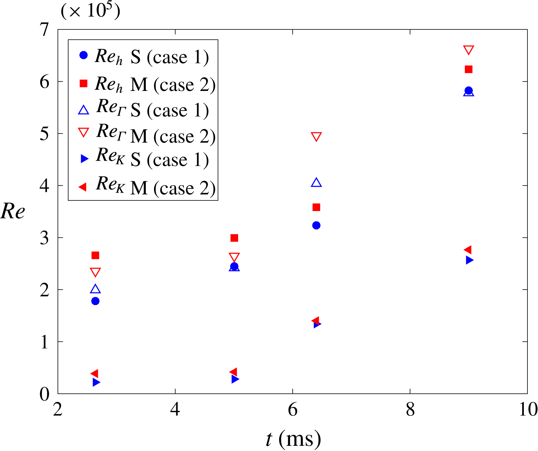
Figure 19 shows the time dependence of each Reynolds number for both single-mode and multi-mode cases. All three methods show a similar trend, as they increase with time at approximately the same rate. This similar trend was expected for
 $Re_{h}$
and
 $Re_{\unicode[STIX]{x1D6E4}}$
because they have similar origins (Jacobs & Sheeley Reference Jacobs and Sheeley1996). Furthermore, Tomkins et al. (Reference Tomkins, Balakumar, Orlicz, Prestridge and Ristorcelli2013) found similar agreement, within a factor of two, between the two methods. Comparatively,
 $Re_{K}$
shows lower magnitudes than the other two, yet displays the same overall trend. As stated by Dimotakis (Reference Dimotakis2000), achieving
 $Re\approx 10^{4}$
is conjectured to be necessary to observe a mixing transition and is a more restrictive condition beyond conditions for turbulent transition. Employing this criterion showed that the Reynolds numbers obtained via the above-mentioned methods satisfy the necessary condition for transition to turbulence at all times.
Temporal Reynolds number values found using three different methods: Mixing width growth rate, total circulation, and total kinetic energy.

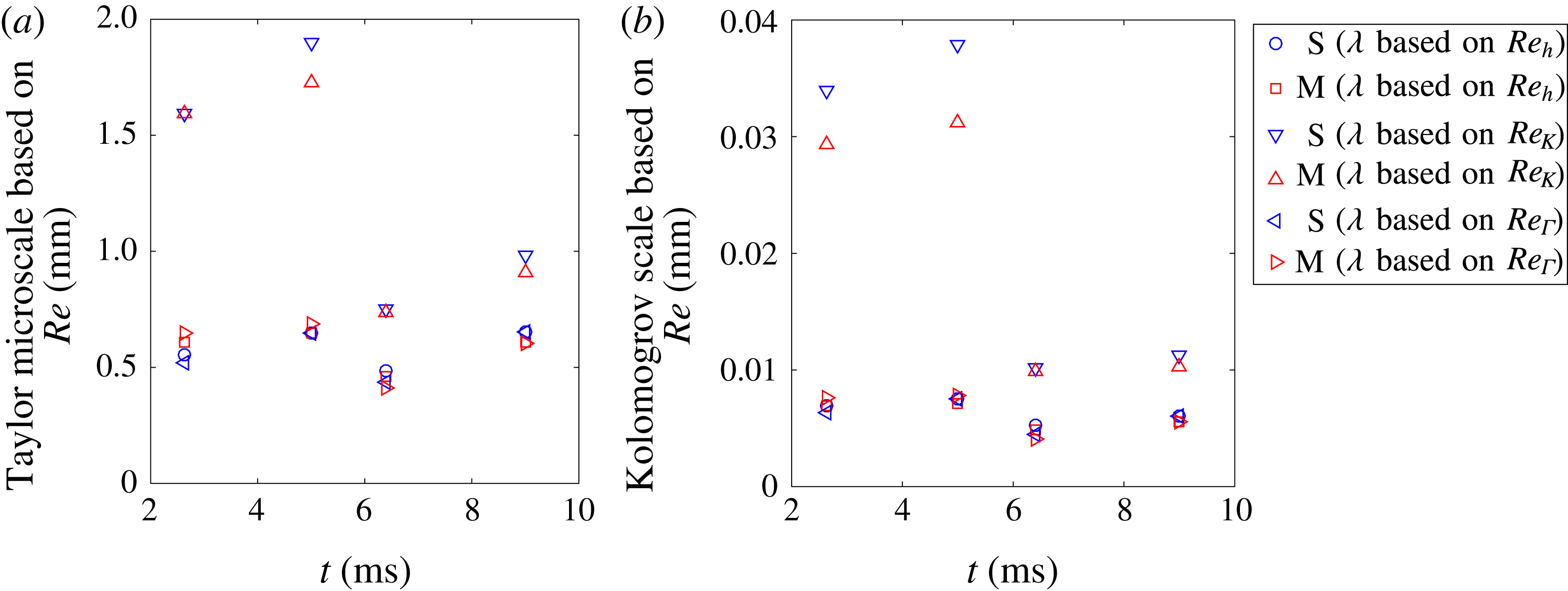
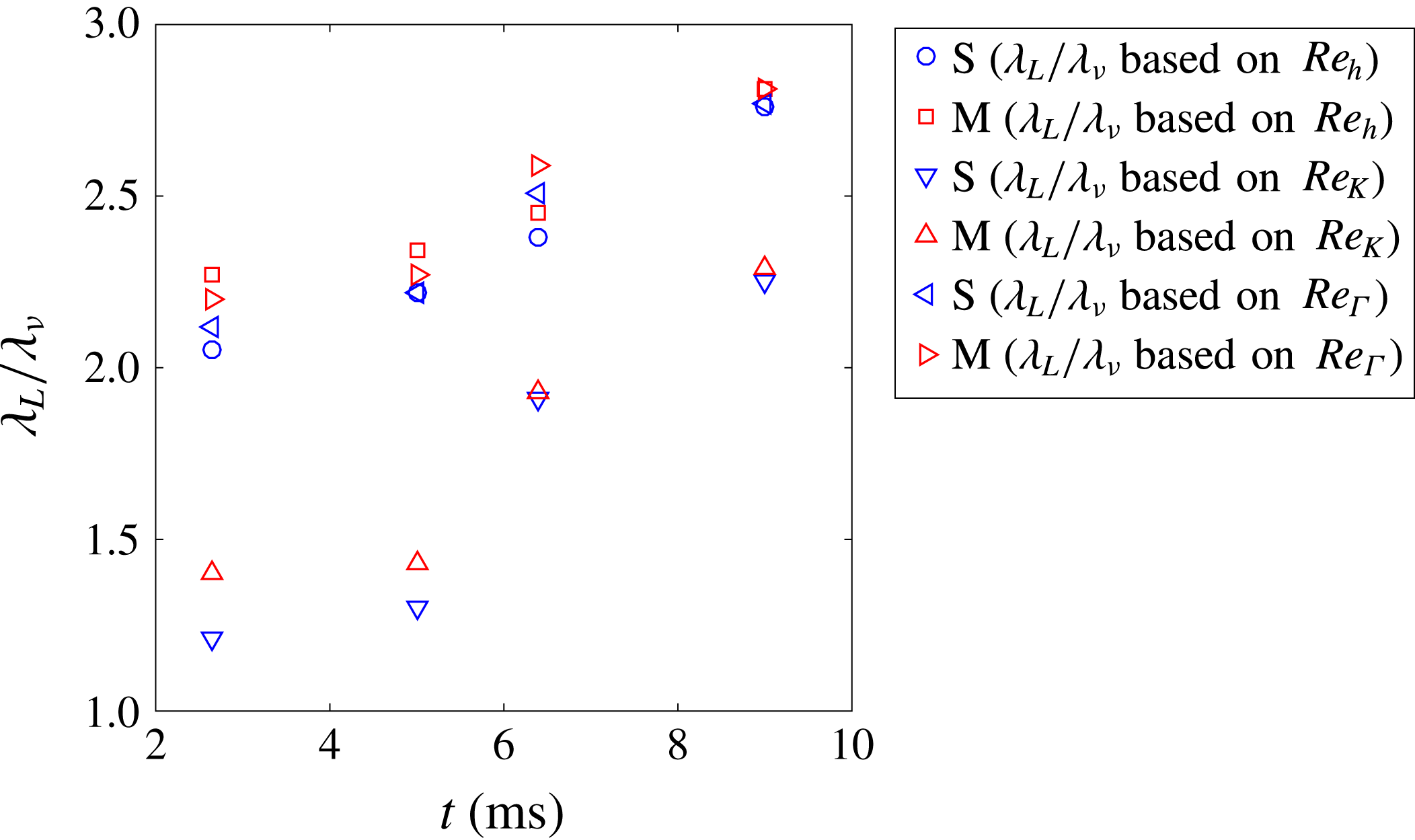
Further information about the energy spectra can be extracted through the Taylor microscale and Kolmogrov scale. These scales can be estimated with a simplifying assumption of local isotropy and knowledge of the Reynolds number values. The Kolmogrov length scale is calculated from the largest length scale in the flow, the mixing width
 $h$
, and the Reynolds number using
 $\unicode[STIX]{x1D706}_{k}\approx hRe^{-3/4}$
. Similarly, the second useful length scale, the Taylor microscale, is
 $\unicode[STIX]{x1D706}_{T}\approx \sqrt{15}hRe^{-1/2}$
(Pope Reference Pope2000; Tomkins et al.
Reference Tomkins, Balakumar, Orlicz, Prestridge and Ristorcelli2013; Orlicz et al.
Reference Orlicz, Balasubramanian, Vorobieff and Prestridge2015).
With information provided by the Kolmogrov scale, one can better estimate in which scales the viscosity is dominant at higher wave numbers. The Taylor microscale gives insight into the inertial sub-range, and allows one to delineate the maximum size of scales which can be assumed to be isotropic and free of influence from large-scale flow features (Robey et al. Reference Robey, Zhou, Buckingham, Keiter, Remington and Drake2003).
By comparing the Taylor microscales derived from Reynolds numbers to those based upon correlation functions, the effects of resolution can be investigated. According to figures 17 and 20, the Taylor microscales measured from velocity correlation functions and spatial gradients are larger by a factor of 3–4 compared to those of
 $Re_{h}$
and
 $Re_{\unicode[STIX]{x1D6E4}}$
, and by a factor of 1.5–2 compared to that of
 $Re_{K}$
. The differences between these methods implies that the resolution effects in velocity could be responsible for the differences. However, comparing Taylor microscales given from the Reynolds number and density correlation function methods (figure 18) shows almost identical results, indicating that the PLIF resolution is fine enough to capture Taylor microscales from density fields.
Other important scales which have been used to show turbulent transition criteria are the Liepmann–Taylor scale (
 $\unicode[STIX]{x1D706}_{L}\approx 5hRe^{-1/2}$
) and the inner viscous scale (
 $\unicode[STIX]{x1D706}_{\unicode[STIX]{x1D708}}\approx 50\unicode[STIX]{x1D706}_{k}$
). The threshold for transition, and therefore the possible presence of an inertial range in the spectra, based on these scales is (
 $\unicode[STIX]{x1D706}_{L}/\unicode[STIX]{x1D706}_{\unicode[STIX]{x1D708}}>1$
), where both scales can be calculated from Reynolds numbers (Dimotakis Reference Dimotakis2000).
Taylor microscale (a) and Kolomogrov scale (b) progressions found with Reynolds numbers derived using three different methods.

Progression of the ratio of Liepmann–Taylor scale to the inner viscous scale provided by Reynolds number values from three different methods.

Values of
 $\unicode[STIX]{x1D706}_{L}/\unicode[STIX]{x1D706}_{\unicode[STIX]{x1D708}}$
computed from the three different Reynolds numbers methods are shown in figure 21. For each of the three calculations, since the fraction is above 1, an inertial range is present, especially after reshock. However, work by Lombardini et al. (Reference Lombardini, Pullin and Meiron2012) suggests that for fully developed turbulence
 $\unicode[STIX]{x1D706}_{L}/\unicode[STIX]{x1D706}_{\unicode[STIX]{x1D708}}$
should be above 10, which is not achieved in the present case. Therefore, based on all discussed above (Reynolds number calculations, the fraction of integral scale to correlation function Taylor microscale, and the fraction of Liepmann–Taylor scale to the inner viscous scale), one can conclude that while a mixing transition is occurring in the present case, especially after reshock, fully developed turbulence is likely not reached.
5.2 Time evolution of energy spectra and structure functions
In order to understand the growth of different scales and to quantify the inertial range, the time evolution of fluctuating kinetic energy, fluctuating enstrophy and the density variance spectra before and after reshock are presented. The general procedure used to compute the spectrum of a quantity
 $\unicode[STIX]{x1D711}(x,y,t)$
(velocity, density or enstrophy fluctuation) is described by Reilly et al. (Reference Reilly, McFarland, Mohaghar and Ranjan2015). Thus, the one dimensional energy spectrum of any quantity is
 $$\begin{eqnarray}\left[E_{\unicode[STIX]{x1D711}^{\prime }}\right]_{i}=FFT(\unicode[STIX]{x1D711}^{\prime })\boldsymbol{\cdot }\text{conj}(FFT(\unicode[STIX]{x1D711}^{\prime })),\end{eqnarray}$$
where
 $FFT(\unicode[STIX]{x1D711}^{\prime })$
is the Fourier coefficient of the
 $2\unicode[STIX]{x03C0}$
periodic function
 $\unicode[STIX]{x1D711}(x,y,t)$
in the spanwise direction and
 $\text{conj}(FFT(\unicode[STIX]{x1D711}^{\prime }))$
is its complex conjugate.
The temporal development of the total fluctuating kinetic energy spectra is computed by adding the
 $u^{\prime }$
and
 $v^{\prime }$
components of the energy spectra for the
 $i$
th column:
 $$\begin{eqnarray}[E]_{i}=[E_{u^{\prime }}]_{i}+[E_{v^{\prime }}]_{i}.\end{eqnarray}$$
Temporal evolution of the combined total fluctuation kinetic energy spectra (a,b), a comparison of compensated spectra at early and late reshock times (c,d), and the normalized cross-correlation spectrum (dashed line fitted with a solid line) (e,f).

The progression of the kinetic energy spectra without
 $w^{\prime }$
component and a comparison of the compensated spectra for the two experimental cases at each time is shown in figure 22. In figure 22(a,b), one can observe oscillations before reshock, especially in the single-mode case at early time (2.64 ms), which are then smoothed by reshock. The spectra increase after reshock (6.4 ms) for both cases, as the second shock adds more energy to the mixing region. Conversely, energy decays after incident shock at 5 ms and at late time after reshock (9 ms). Compensated spectra are also shown in figure 22(c,d), where the compensation exponent,
 $n$
, is shown in the legend. Because the out-of-plane component of velocity is unknown, the spectra is compared to that of the inertial sub-range scaling of both (
 $-5/3$
) and (
 $-3$
) predicted by 3D and 2D classical turbulence, respectively. It is important to note the assumptions of classical spectra are that the flow is both isotropic and incompressible. The flow is fairly incompressible after passage of shock, but is anisotropic and inhomogeneous. However, similar to Schilling et al. (Reference Schilling, Latini and Don2007) and Orlicz et al. (Reference Orlicz, Balasubramanian, Vorobieff and Prestridge2015), the scalings associated with classical turbulence of expected power laws of
 $5/3$
, for the small, energy-containing wave numbers, and 3, for larger wave numbers are used to compensate the velocity fluctuation spectra. Once compensated, a full decade (
 $k_{y}\approx 200$
–2000) of the inertial range approximately follows the
 $-5/3$
law after reshock, at 6.4 and 9 ms. However, less than half a decade of spectra in the large wave numbers is observed to approximately follow the
 $k^{-3}$
power law. This is likely an effect of resolution limitation and not a physical dissipation range. The compensated energy spectra is used to emphasize the separation between large and small scales which is another indication of transition to turbulence (Zhou Reference Zhou2017).
In order to investigate the level of anisotropy and memory of initial conditions across different scales with time for both single and multi-mode cases, the normalized cross-correlation spectrum between
 $u^{\prime }$
and
 $v^{\prime }$
,
 $|E_{u^{\prime }v^{\prime }}(k_{y})|/[E_{u^{\prime }u^{\prime }}(k_{y})E_{v^{\prime }v^{\prime }}(k_{y})]^{1/2}$
, is considered in figure 22(e,f) (Tavoularis & Corrsin Reference Tavoularis and Corrsin1981a
,Reference Tavoularis and Corrsin
b
; Shen & Warhaft Reference Shen and Warhaft2000). Anisotropy is clearly present before reshock (2.64 and 5 ms) in the single-mode case even at smaller scales; however, in the multi-mode case, the tendency toward isotropy of small scales is evident as the wave number increases. This local isotropy in the multi-mode case also suggests that memory of the initial condition is maintained before reshock (both 2.64 and 5 ms) because imposed perturbations in the IC causes a tendency toward isotropy in mid-range scales. After reshock (6.4 and 9 ms), the cross-correlation spectrum decays more rapidly in both single- and multi-mode cases, which indicates that local isotropy is reached at lower wave numbers than before reshock. The decrease in normalized cross-correlation spectrum from 6.4 ms to 9 ms in both cases at larger scales is an indicator of breakdown of large scales to small scales between 6.4 and 9 ms. Comparison of single- and multi-mode cases at 6.4 and 9 ms shows the similarity between imposed scales in the initial condition and the scales which result from breakdown of large to small scales upon reshock. Thus, a significant range of scales exists which are locally isotropic in both cases, and the anisotropy is primarily contained in the large scale which is common to the two cases.
The fluctuating enstrophy is defined as
 $(\unicode[STIX]{x1D714}^{\prime })^{2}/2$
and its time evolution is seen in figure 23(a,b), which also shows the compensated spectra for both of the cases after reshock (figure 23(c,d)), similar to the velocity energy spectra in figure 22. While the slope of fluctuating enstrophy spectra is lower than velocity spectra, it is similar to the velocity energy spectra in that it is again amplified by reshock. An additional similarity is that the enstrophy spectra also decays at late time after the incident shock (5 ms).
Temporal evolution of the fluctuation enstrophy spectra (a,b) and a comparison of compensated spectra at early and late reshock times (c,d).

The fluctuating enstrophy spectra in homogeneous, isotropic flow (classical turbulence) can be related to velocity spectra via
 $E_{\unicode[STIX]{x1D714}^{\prime }\unicode[STIX]{x1D714}^{\prime }}(k,t)=k^{2}E(k,t)$
. The expected slope of the inertial range in the fluctuating enstrophy spectra will be
 $1/3$
at small wave numbers and
 $-1$
at large wave numbers for 3D turbulence. Moreover, according to Batchelor (Reference Batchelor1969) and Kraichnan (Reference Kraichnan1967), the energy spectra of classical 2D turbulence scales with
 $k^{-3}$
, which yields
 $-$
1 scaling for enstrophy spectra at inertial range scales. Therefore,
 $-$
1 scaling in the enstrophy spectrum can be compared with both classical 3D turbulence at larger wave numbers and classical 2D turbulence at smaller wave numbers (Kraichnan Reference Kraichnan1967; Batchelor Reference Batchelor1969). Figure 23(c,d) shows approximately
 $k^{-1}$
scaling in the compensated spectra for less than one decade after reshock; however, the largest scales show scaling close to
 $k^{1/3}$
for almost one decade (
 $k_{y}\approx 20$
–200).
Structure functions were calculated in order to find the inertial ranges and slopes of spectra so they could be compared with those from different spectra. The second-order longitudinal structure function is
 $S_{2}(r)=\langle (\unicode[STIX]{x1D702}(x+r)-\unicode[STIX]{x1D702}(x))^{2}\rangle$
, where
 $\unicode[STIX]{x1D702}$
is the velocity or density fluctuation in the direction of the separation length,
 $r$
, and brackets
 $\langle \rangle$
denote both spatial and ensemble averaging.
Temporal evolution of the velocity structure function (a,b) and a comparison of compensated structure function at early and late reshock times (c,d).

Figure 24 shows the time evolution of the velocity structure functions for each case (a,b), as well as the comparison between the compensated structure functions after reshock (c,d). The decay of the small-scale contribution can be seen during both pre- (2.64–5 ms) and post-reshock (6.4–9 ms) for the single- and multi-mode cases. In addition, the large scale peak is similarly dampened at 5 and 9 ms for both cases. Analyzing the compensated structure functions after reshock shows a slope close to that of the
 $2/3$
power law of Kolomogorov turbulence (classical turbulence) for almost an entire decade.
The temporal development of the density fluctuation spectrum and the comparison of compensated spectra for each case after reshock are shown in figure 25(a,b) and (c,d), respectively. Unlike the velocity fluctuation spectra, there is a small increase in the density spectra after incident shock, between 2.64 and 5 ms, and after reshock, between 6.4 and 9 ms, especially at small scales. Yet, similar to the velocity spectra, reshock sharply increased the spectra magnitude, which suggest that density fluctuations are stronger post-reshock. Classical scaling of
 $-5/3$
is again of interest, even for density spectra. Therefore, the assumption of isotropy at small scales should hold true in order to have the same scaling as a classical spectra. Some researchers have found similar scaling for density spectra even with inhomogeneous and unsteady flow, which is not assumed in the classical case (Vorobieff, Rightley & Benjamin Reference Vorobieff, Rightley and Benjamin1998). In the current case, the density fluctuation spectrum shows an approximate
 $k^{-5/3}$
scaling for half a decade at intermediate wave numbers after reshock, as shown by the compensated spectra. There is a small increase in the inertial range which can be seen from 6.4 ms (early reshock) to 9 ms (late time after reshock). Furthermore, these results are verified by density fluctuation structure functions which are shown in figure 26. Post-reshock, density fluctuation structure functions also show close to
 $2/3$
scaling for intermediate
 $r$
and for less than a decade.
Temporal evolution of the density spectra (a,b) and a comparison of compensated spectra at early and late reshock times (c,d).

Temporal evolution of the density structure function (a,b) and a comparison of compensated structure function at early and late reshock times (c,d).

6 Conclusions
Variable-density turbulence resulting from RMI was studied to investigate turbulent mixing and its dependence on initial conditions. Using simultaneous PLIF-PIV diagnostics, an interface between a nitrogen-acetone mixture and carbon dioxide (Atwood
 ${\sim}$
0.22) which initially contained small wavelength, multi-mode secondary perturbations was compared to that of the large-wavelength single-mode perturbation initial condition before (2.64 and 5 ms) and after reshock (6.4 and 9 ms) at incident shock Mach number
 ${\approx}1.55$
.
Before reshock, comparison of the single- and multi-mode case using density and velocity statistics, such as mixing width, mixedness, density self-correlation, anisotropy, vorticity, and normalized cross-correlation spectrum, provide evidence that the flow shows a distinct memory of the initial conditions. In both cases the long-wavelength perturbation has a strong influence on the interface development before and after reshock because the overall entrainment, stretching, and overturning occur at this large scale. The coherence of the large-wavelength spike and bubble features in the density field even after reshock leads to the conclusion that the memory of the largest scales is maintained.
After reshock, the reflected shock wave deposits additional vorticity which is two to three times higher than the initial vorticity deposition. The resulting disordered vorticity field produces small-scale perturbations similar to those present in the multi-mode initial condition, which then causes an apparent loss of memory of the initial condition at small wavelengths. However, the memory of the initial condition is still observed after reshock, as indicated by the distribution of small-scale structures along the interface, and in the positive and negative vorticity distributions which correspond with the density gradients of the small-scale structures as shown in figure 10. Furthermore, the multi-mode case is observed to have less intense gradients and be more well mixed at all times even after reshock. The multi-mode case displayed higher positive circulation at all times, while the single-mode case showed higher negative circulation. This difference between the two cases results from the interaction of the initial shock and reshock with a more unidirectional density gradient in the single-mode case but with a multidirectional density gradient in the multi-mode case.
In order to confirm that these initial condition remnants occurred in a state of transition to turbulence in the mixing layer after reshock, the following points are investigated:
-
(1) According to Dimotakis (Reference Dimotakis2000), the Reynolds number threshold for a transition to turbulence to be possible is
 $10^{4}$
. This criteria was found to be satisfied at all times for both initial conditions.
-
(2) Another important turbulent transition criterion, which shows the possibility of the presence of an inertial range, is the ratio of the Liepmann–Taylor scale to the inner viscous scale, which should be larger than 1 (
$\unicode[STIX]{x1D706}_{L}/\unicode[STIX]{x1D706}_{\unicode[STIX]{x1D708}}>1$
) (Dimotakis Reference Dimotakis2000). This criterion was also satisfied at all times for both cases. However, to achieve fully developed turbulent flow, Lombardini et al. (Reference Lombardini, Pullin and Meiron2012) suggests that this fraction should be larger than 10, which is not attained in this experiment. In the case of the study by Lombardini et al. (Reference Lombardini, Pullin and Meiron2012), it was found that this threshold was only met for a Mach number greater than 3. -
(3) The energy spectra of the velocity, enstrophy and density fluctuations show inertial range formation for approximately one decade, which is further evidence of the transition to turbulence after reshock. Additionally, similar inertial ranges are formed in the second-order structure functions of velocity and density fluctuations which are consistent with the results of the energy spectra.


Turbulent length scales were measured from small scales using correlation function and spatial gradient methods (which are dependent on resolution), and then they were compared with length scales extracted from larger-scale measurements by means of various Reynolds number calculation methods. Results suggest that the resolutions of density fields are fine enough to capture Taylor microscale; however, Taylor microscales which were computed from velocity correlation functions are larger by a factor of 3–4 compared to those from the Reynolds number.
In both cases after reshock, local isotropy is demonstrated by the normalized cross-correlation spectra at most scales smaller than the inclined perturbation scale. Many measurements presented in the current work have shown that the additional perturbations of the multi-mode case, which have an obvious effect on early flow development, are also remembered after reshock despite development of local isotropy at the scales of these perturbations and evidence that the flow is transitioning to turbulence.
Acknowledgements
The authors are grateful to Vladimer Tsiklashvili for all his assistance in experiments and R. Mejia-Alvarez for his guidance regarding POD analysis. This work was partially supported by the National Science Foundation Faculty Early Career Development (CAREER) Award (award no. 1451994) and Air Force Office of Scientific Research Young Investigator Research Program (AFOSR-YIP, grant no. FA9550-13-1-0185).
Appendix A. Process to register PLIF fields with PIV data
This section is provided to outline the process used to obtain registered fields. Figure 27 shows a visual representation of PLIF processing and describes the steps. As stated before, the procedure is derived from Collins & Jacobs (Reference Collins and Jacobs2002), Weber et al. (Reference Weber, Haehn, Oakley, Rothamer and Bonazza2012, Reference Weber, Haehn, Oakley, Rothamer and Bonazza2014). In order to capture the same field of view and maintain resolution, it is necessary that at least one of the cameras be angled. It was found that if a configuration is chosen such that the PIV camera was angled in relation to the laser sheet using a scheimpflug mount (with the PLIF camera perpendicular) the velocity statistics, especially vorticity, yielded a high error due to out-of-plane motion which can not be distinguished from in-plane-motion using only one offset PIV camera (it is possible in stereo PIV). Fortunately, a comparison of the resulting density profiles from the PLIF camera in the angled and the perpendicular orientation resulted in
 ${<}2$
% difference. Therefore, the PLIF camera with a scheimpflug mount was angled in relation to the laser sheet, with the PIV camera perpendicular, for the experimental setup.
PLIF/PIV Processing: (a) A sample PLIF image as collected. (b) Image of the two-plane calibration plate which is used to correct for lens and perspective effects and to align the PLIF image to the PIV vector field. (c) PLIF image after dewarping is performed to correct lens and perspective effects. (d) PLIF image after correction for decrease in intensity at radial locations farther from the cylindrical lens due to divergence and for Beer–Lambert attenuation due to absorption. The image has been transformed in a way that does not decrease resolution in order to make rays parallel so that streaks appear as high-frequency content in only one direction and low-frequency content in the other. (e) Final processed PLIF image after filtering of high-frequency streaks due to index of refraction mismatch across the interface and reversing the aforementioned transformation. (f) An example showing 25 % of vectors registered to the final PLIF image.

Furthermore, the density and velocity fields must be reconciled accurately, so registering the separate PIV and PLIF results is a crucial step in the analysis. To register the results and images from each of these cameras, the calibration plate seen in figure 27(b) was used. The plate was made so that each white dot is separated precisely by 10 mm in the
 $X$
and
 $Y$
directions and a depth of 1 mm in the
 $Z$
direction. To complete the calibration process, the plate was aligned with the laser light-sheet and illuminated with an external light source so each dot was clearly visible and focused. The plate was positioned such that each camera was able to capture its entirety. After capturing calibration images, a third-order polynomial mapping function was used, as in Soloff, Adrian & Liu (Reference Soloff, Adrian and Liu1997), to map the white dot locations on the image plane to their true measurement locations on the calibration plate in order to correct lens effect. After calibrating the images for both PLIF and PIV cameras separately, the two images are registered to the same coordinate plane by first shifting the fiducial point and using the corner dots to determine the scaling between the two images. Then the spatial region, which is not common to both velocity and density fields, is cropped. The result is that the two fields represent the same spatial region, but maintain the original resolution for calculations.
Appendix B. Instantaneous and statistical uncertainty analysis
Despite the aforementioned efforts to maximize fidelity of the present experiments, it is important to provide analysis of the sources and magnitude of error in the current work. The instantaneous uncertainty in the vector field was estimated to be 1 % using the Primary Peak Ratio (PPR) method, which is the ratio of the primary correlation peak to the strongest secondary correlation peak. Image quality, in-plane and out-of-plane motions affect peak ratio (Charonko & Vlachos Reference Charonko and Vlachos2013; Tomkins et al. Reference Tomkins, Balakumar, Orlicz, Prestridge and Ristorcelli2013; Xue, Charonko & Vlachos Reference Xue, Charonko and Vlachos2014). Instantaneous error in the density measurements results from shot-to-shot noise, variations in extinction coefficient, and index of refraction effects on the light sheet. The shot noise is approximately 2 % of the intensity range, acetone concentration is maintained constant and uniform in the light gas to provide consistency in the extinction coefficient, and the index of refraction effects are corrected to the ability of current procedures. The resulting error in the instantaneous density fields is estimated to be less than 10 % (Balakumar et al. Reference Balakumar, Orlicz, Ristorcelli, Balasubramanian, Prestridge and Tomkins2012).
Regarding statistical uncertainty analysis, velocity, density, and the corresponding derived statistics are random variables which are generally functions of space and time. Due to this, the central limit theorem suggests that the rate of statistical convergence is dependent upon the square root of the mean square error (MSE) or, alternatively, the standard deviation of the estimator (Bendat & Piersol Reference Bendat and Piersol2011),
 $$\begin{eqnarray}\sqrt{var(\hat{\unicode[STIX]{x1D719}}(x))}=\unicode[STIX]{x1D70E}_{\hat{\unicode[STIX]{x1D719}}}=\sqrt{\frac{\unicode[STIX]{x1D70E}_{\unicode[STIX]{x1D719}}^{2}}{N_{i}}},\end{eqnarray}$$
where
 $\hat{\unicode[STIX]{x1D719}}(x)$
is the estimator for any statistics of the random variable
 $x$
and
 $N_{i}$
is the total number of independent samples. For example, the sample mean
 $\bar{u}$
is an estimator for the population mean
 $u$
-component velocity,
 $\unicode[STIX]{x1D707}_{u}$
. In this case
 $\hat{\unicode[STIX]{x1D719}}=\bar{u}$
and
 $\unicode[STIX]{x1D70E}_{\unicode[STIX]{x1D719}}^{2}=\unicode[STIX]{x1D70E}_{u}^{2}$
.
 $N_{i}$
appears in the denominator, and hence convergence of any specific statistic is dependent on the number of realizations. Variances for the estimators of the statistics of interest were derived previously (Benedict & Gould Reference Benedict and Gould1996; Balakumar et al.
Reference Balakumar, Orlicz, Ristorcelli, Balasubramanian, Prestridge and Tomkins2012) and are shown in table 2. For each of the statistics, confidence intervals may be formed following the method of Benedict & Gould (Reference Benedict and Gould1996),
 $$\begin{eqnarray}\unicode[STIX]{x1D719}=\hat{\unicode[STIX]{x1D719}}\pm z_{\unicode[STIX]{x1D6FC}}\sqrt{\frac{\unicode[STIX]{x1D70E}_{\unicode[STIX]{x1D719}}^{2}}{N_{i}}},\end{eqnarray}$$
where
 $z$
is the
 $z$
-score for the normal distribution at the desired confidence interval (
 $\unicode[STIX]{x1D6FC}$
), which was 95 % for this study. Typical confidence intervals (CI) and one (
 $\unicode[STIX]{x1D70E}$
) relative error (RE) level are shown in table 2.
Definitions, equations and convergence of statistical estimations.
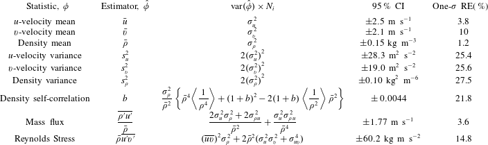
The experiment was repeated at fixed times after the arrival of the incident shock to produce independent ensembles. Small variations in particle and acetone density, shock velocity, image quality, and other experimental aspects make achieving identical conditions difficult. Although every effort was made to mitigate these variations, approximately 30 realizations were completed per test time for each initial condition at most experimental times in order to ensure minimal influence from these variations on the data set and to allow calculation of ensemble statistics. Approximations for the estimator variance and standard errors were calculated using
 $N_{i}\approx 30$
. Furthermore, after averaging over the ensemble, many statistics are averaged in the spanwise direction to produce a profile against streamwise coordinates. This implies an assumption of spatial homogeneity across the layer. This assumption is typically accepted when a limited number of realizations are available (Shankar & Lele Reference Shankar and Lele2014), and is necessary for comparison with many simulations and other experimental work. An initial calculation found the integral length scale,
 $L$
, to be
 $L\approx 1.0$
cm, which was used to identify the length of independence in the spatial field. Therefore, the spanwise length, (
 ${\approx}10~\text{cm}$
), yields close to 10 independent samples per ensemble and about 300 total for the spanwise-averaged calculations at most experimental times.
Appendix C. Additional insights into the state of the flow
C.1 Dissipation rate and mean density profile
This section gives further insights into the density field evolution through a description of dissipation rate, and mean density profiles. The scalar dissipation rate,
 $\unicode[STIX]{x1D712}=D(\unicode[STIX]{x1D6FB}\unicode[STIX]{x1D709}.\unicode[STIX]{x1D6FB}\unicode[STIX]{x1D709})$
, is a measure of the rate of molecular mixing which occurs on the smallest scales. As mentioned earlier, the PLIF resolution is not sufficient to capture the Batchelor scale, so the dissipation rate is filtered to the resolution, and thus will likely underestimate dissipation rate. The dissipation rate would be zero for immiscible fluids, although they are capable of entrainment at slightly larger length scales. Molecular mixing serves to homogenize the flow and is thus critical to the development of the interface, as the strength of gradients affects secondary instability development and the early vorticity field resulting from reshock. The scalar dissipation rate calculated assuming a constant diffusivity is shown in figure 28. At each of the experimental times presented, the single-mode case displays a higher rate of dissipation in most of the mixing region. The two times before reshock highlight a major difference between the single-mode and multi-mode cases; the deposition of vorticity in many directions onto the multi-mode interface contorts the scalar dissipation field leading to a much less organized field, and consequently lower dissipation rates over a larger area. The dissipation rates on the spike side due to the penetration of fresh mass and shearing of mixing mass are slightly higher than in the bubble region, whereas in the single-mode case where less mixed mass is available to be stripped off, the dissipation rate is approximately the same along the length of the interface. The comparison is similar after reshock as well, although there is less dissipation overall due to smearing of gradients by turbulent motion.
Dissipation rate evolution for both cases. S refers to single-mode case and M refers to multi-mode case.

Profiles of the density fields, which were averaged in the spanwise direction and averaged over the ensemble, are shown in figure 29. There is a small difference between 2.64 and 5 ms due to the increase in mixed width from interface stretching. There is a noticeable difference at 5 ms between the two cases, where the shear rollup causes a local peak at about 1.9 cm in the single-mode case. The increase in density and the increase in the density contrast between the two gases caused by reshock is obvious. Less obvious is any difference between the two cases at 6.4 ms; the single-mode case has a slightly steeper transition on the light gas side. The overturning of the interface is pronounced for both cases from 6.4 ms to 9 ms as the mixing layer encompasses a larger region. The multi-mode case has a predominantly linear profile at 9 ms while the single-mode case has a slight deviation from a linear trend near the centre of mass due to a heavy-gas feature which is more consistently present.
Temporal evolution of the mean density profiles at each time.

C.2 Circulation
This section gives further insights into the velocity field evolution through description of circulation. Concerning vorticity and circulation, two separate methods were used in order to verify the procedures and results. First, vorticity was computed by taking the curl of the 2D velocity vector field (
 $\unicode[STIX]{x1D714}=\unicode[STIX]{x1D735}\times V$
) at each point in the field. This method is identical to the process used in Reilly et al. (Reference Reilly, McFarland, Mohaghar and Ranjan2015). Next, for comparison and verification, vorticity was back-calculated from circulation: a local circulation for each point in the velocity fluctuation field was found using
 $$\begin{eqnarray}\unicode[STIX]{x1D6E4}(t)=\int _{C}\boldsymbol{V}\boldsymbol{\cdot }\,\text{d}\boldsymbol{r},\end{eqnarray}$$
where the velocity field is integrated around a closed interval
 $C$
, which encompasses the entire cropped region of the velocity field. This method is similar to the one used in Schilling et al. (Reference Schilling, Latini and Don2007) and Weber et al. (Reference Weber, Haehn, Oakley, Rothamer and Bonazza2014), which was shown to have good agreement with the Samtaney–Zabusky model, but the encompassing region of
 $C$
is altered. The above integral was broken up into the sum of many small integrals with regions of
 $C$
that encompass individual points in the velocity field. The velocity differences along each line segment making up the small area
 $S$
(with a size of
 $2\times 2$
vectors) result in a ‘local circulation’ about the centre of each region. The total circulation is then the sum of these ‘local circulations’ calculated from individual points in the velocity fluctuation field. From this point the following relation is used to find the vorticity
 $$\begin{eqnarray}\unicode[STIX]{x1D6E4}(t)=\int \int _{S}\unicode[STIX]{x1D74E}\boldsymbol{\cdot }\text{d}\boldsymbol{S}.\end{eqnarray}$$
Thus, by dividing each local circulation value by the area,
 $\text{d}\boldsymbol{S}$
, of the encompassing region
 $C$
, a vorticity field is generated from the circulation of the flow field. Evaluating the integral in this way allows for the size and shape of the region
 $C$
to be selected to achieve further smoothing in the vorticity field, if desired. The results of these two methods produce vorticity fields that are essentially identical.
Positive, negative and total circulation. The error bar at each time represents
 $\pm$
one standard deviation.

Results from the circulation data can help to understand the vorticity field evolution, as the circulation is merely the result of vorticity deposition (Schilling et al. Reference Schilling, Latini and Don2007). The positive, negative, and total circulation in the flow field at each time is displayed below in figure 30(a–c). Due to the relation between vorticity and circulation, by comparing figure 30(a,b), it can be confirmed that the negative vorticity components in the multi-mode and single-mode cases are of a greater amplitude than the positive components (for case S, positive circulation, and thus positive vorticity is essentially negligible). After the incident shock wave passes, both negative and positive circulation components can also be seen to increase very slightly, as was expected from the vorticity analysis. For both cases, the greatest increase in positive circulation comes immediately after reshock. This is to be expected as it corresponds to when the greatest amount of positive vorticity is deposited within the flow field. Comparatively, the greatest increase in negative circulation occurs as the reshocked interface perturbations grow. It should also be noted that the growth rate of vorticity and circulation (both positive and negative) post-reshock, between 5 and 6.4 ms, is greater in the single-mode case than in the multi-mode case, yet total circulation shares a very comparable trend for both.
C.3 Normalized anisotropy tensor magnitude
Temporal evolution of
 $\unicode[STIX]{x1D6FD}_{11}$
for both single-mode and multi-mode cases.

This section gives further insights into the cross statistics through a description of normalized anisotropy tensor magnitude. The spanwise average of
 $\unicode[STIX]{x1D6FD}_{ij}$
obscures the total anisotropy as it averages both positive and negative values over the span. Since ensemble averaging is used the values across the span are not correlated by their average. Figure 31 shows the spanwise average of the magnitude of the anisotropy tensor
 $\Vert \unicode[STIX]{x1D737}\Vert$
:
 $$\begin{eqnarray}\Vert \unicode[STIX]{x1D737}\Vert =\unicode[STIX]{x1D6FD}_{ij}\unicode[STIX]{x1D6FD}_{ij}.\end{eqnarray}$$
 $\Vert \unicode[STIX]{x1D737}\Vert$
is positive everywhere, accounts for all three directions, and diminishes to zero as the flow becomes isotropic. From figure 31, a clear trend emerges over time for the two cases. Both cases show a high degree of anisotropy at early times, as expected, but the multi-mode case shows a much lower anisotropy before reshock, at 5 ms. The anisotropy remains lower for the multi-mode case after reshock. The single-mode case does not show low values until after reshock.