1. INTRODUCTION
Ambiguity resolution is crucial to precise Global Navigation Satellite System (GNSS) applications. It has attracted a great deal of attention from the GNSS community in the past two decades. Various methods have been developed to solve for the integer ambiguities, such as the extra-widelaning technique (Wübbena, Reference Wübbena1989), ambiguity function method (Counselman and Gourevitch, Reference Counselman and Gourevitch1981), fast ambiguity resolution approach (Frei and Beulter, Reference Frei and Beulter1990), Cholesky decomposition (Euler and Landau, Reference Euler and Landau1992), least squares (LS) ambiguity searching technique (Hatch, Reference Hatch1990) and the Least squares AMBiguity Decorrelation Adjustment (LAMBDA) (Teunissen, Reference Teunissen1993). The popularity of the LAMBDA method stems from its numerical efficiency and its guaranteed optimality in the sense of maximising the probability of correct integer ambiguity estimation (Teunissen, Reference Teunissen1999).
In the past two decades, the LAMBDA method has been used for applications in which the ambiguity dimension is in the order of several tens. With the advent of denser network processing and multi-frequency, multi-GNSS tracking, the ability to deal with much higher ambiguity dimension is required. This contribution is the first attempt to analyse LAMBDA's performance in high dimensional search spaces. By embedding the LAMBDA method into the Bernese software (version 5.0), the ambiguity resolution performance can be compared and evaluated. The evaluation includes the numerical efficiency of the decorrelation and the search steps of LAMBDA itself and the effect of the LAMBDA integer solution on the baseline precision (i.e. baseline repeatability). It should be noted that our analyses in this contribution are only the first step due to the fact that: (i) we use the LAMBDA method only as a full ambiguity resolver (i.e. no partial ambiguity resolution is examined) and (ii) the LAMBDA results are not validated, e.g. without the fixed failure-rate ratio test (Teunissen and Verhagen, Reference Teunissen and Verhagen2009).
The structure of the rest paper is as follows. In Section 2, a brief review is given of integer LS estimation and the LAMBDA method. In Section 3, the Bernese quasi-ionosphere-free (QIF) ambiguity resolution method is described. The experimental results and analyses for the LAMBDA's performance are presented in Section 4. Finally, some concise concluding remarks are given in Section 5.
2. INTEGER LEAST SQUARES AMBIGUITY RESOLUTION AND LAMBDA METHOD
2.1. Integer least squares ambiguity estimation theory
All the linearized GNSS observation equations can be generalized as:

where the observation vector y∈Rn contains the observed-minus-computed pseudorange and carrier-phase observables; the observation noise vector e is usually assumed to be normally distributed with zero mean and variance-covariance matrix Q y; The vector a∈Zm is for unknown carrier-phase integer ambiguities, and the vector b∈Rp for other real-valued unknown parameters, which usually includes baseline components and possibly tropospheric and ionospheric parameters; The matrices A and B are the known design matrices to a and b, and both of them generally have full column rank. Based on the LS criterion, the equation system (1) is solved by means of the minimisation problem:

Generally, the following three-step procedure is employed for solving the minimisation problem (2). In the first step, the integer property of a is disregarded and the float solution and its variance-covariance matrix are computed:
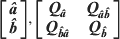
In the second step, the float ambiguities are mapped into integers by setting up a new minimisation problem:

In the third step, the real-valued parameters  solved from the first step are updated using the fixed integer ambiguities
 from the second step:

For the ambiguity-fixed solution  having a better precision than its float counterpart , the success probability of integer ambiguity solution must be sufficiently close to 1 (De Jonge et al, Reference De Jonge, Teunissen, Jonkman and Joosten2000).
2.2. The LAMBDA method
In the LAMBDA method, the integer solution to (4) is found by means of an efficient search over the ellipsoidal search space defined as

The search speed depends on the size χ 2 and the shape of the ellipsoid. The positive constant χ 2 can be predetermined using different strategies (De Jonge and Tiberius, Reference De Jonge and Tiberius1996) and then gradually shrunk during the search (Chang et al, Reference Chang, Yang and Zhou2005; De Jonge and Tiberius, Reference De Jonge and Tiberius1996; Teunissen, Reference Teunissen1993, Reference Teunissen1995b). The shape and orientation of the ellipsoid are defined by the variance-covariance matrix  of the float ambiguity estimates. Since a high correlation among the ambiguities may lead to search halting which in turn makes the search time-consuming, the decorrelated ambiguities are used instead of the original ones in the LAMBDA method (Teunissen, Reference Teunissen1993). After decorrelation, the original ambiguities are transformed to the decorrelated ones using z=ZTa, and then the search is conducted in the transformed ellipsoid:

where  and
 . Let the triangular factorisation of the decorrelated variance-covariance matrix be
 , the search over the ellipsoid (7) is then based on the evaluation of the scalar interval:

with
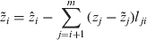
where L is a unit lower triangular matrix and l ji (j > i) is its element of the jth row and the ith column; D is a diagonal matrix whose ith element,  , is the conditional variance of the ith transformed ambiguity z i conditioned on the transformed ambiguities I={i+1, …, m}. Based on these bounds (8), the search is performed. For more details on the LAMBDA method, one refers to Teunissen (Reference Teunissen1993, Reference Teunissen1995a, Reference Teunissenb), De Jonge and Tiberius (Reference De Jonge and Tiberius1996), Strang and Borre (Reference Strang and Borre1997), Teunissen and Kleusberg (Reference Teunissen and Kleusberg1998), Hofmann-Wellenhof et al (Reference Hofmann-Wellenhof, Lichtenegger and Collins2001) and Leick (Reference Leick2004).
3. BERNESE AMBIGUITY RESOLUTION AND ITS TRANSFORMATION
3.1. Quasi-ionosphere-free ambiguity resolution strategy in Bernese
Several ambiguity resolution strategies are available in the Bernese software package. The optimal strategy is determined by many factors including the baseline length, session length, and so on. The quasi-ionosphere-free (QIF) strategy is used to solve ambiguities of baselines over several hundred kilometres long. The criterion used in the QIF strategy is to minimise the difference between the real-valued and integer ionosphere-free biases (IFBs).
In the QIF algorithm, the L1 and L2 ambiguities are fixed as a pair. Firstly, the IFB standard deviations of all pairs of the original DD float ambiguities and the newly formed DD float ambiguities with changed reference satellite are computed based on the variance-covariance matrix of float ambiguity estimates. Then the ambiguity fixing process starts from the ambiguity pair with the smallest IFB standard deviation. Its integer candidates are defined by the integer candidates of L1 and widelane ambiguities. The pair of integer candidates with the smallest difference between the real-valued and integer IFBs is accepted as the optimal solution, as long as such a difference is smaller than the user-defined maximum value. Once such a pair of integer candidates is accepted, the entire sequential LS adjustment and the procedure described above are repeated so that all or some of the ambiguity pairs are fixed. More details can be found in Dach et al (Reference Dach, Hugentobler, Fridez and Meindl2007).
3.2. Ambiguity transformation in QIF
The Bernese software works not only with original DD ambiguities, but also with transformed DD ambiguities with changed reference satellites. Thus, the fixed ambiguities in QIF are in fact the transformed ambiguities from the original ambiguities. This transformation can be symbolised as:
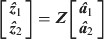
where  and
 are the original DD float ambiguities at the L1 and L2 frequencies respectively. Since the L1 and L2 ambiguities, as a pair, are fixed simultaneously, the Z-transformation matrix has structure

where ZB is used to transform the DD ambiguities at one frequency by changing the reference satellite. All elements in one row of ZB are in either case: (i) 0 except one 1 to retain the original DD ambiguity; (ii) 0 except one 1 and one –1 to form the new DD ambiguity. For instance, the ZB is given for the four DD ambiguities as:
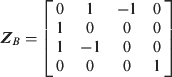
In this case, the newly formed DD ambiguities,  and
 with respect to the L1 and L2 frequencies, are first fixed simultaneously because their associated IFB standard deviation is smallest.
It is emphasised that the fixed ambiguities in Bernese are the transformed ambiguities in terms of (10) rather than the original DD ambiguities. Furthermore, only part of the transformed ambiguities that meet the user-defined conditions can be fixed. Thus, the dimension of Z is t-by-m with generally t⩽m.
4. EXPERIMENT RESULTS AND ANALYSIS
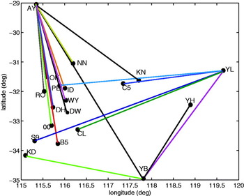
The experiment was conducted using the 24-hour dual-frequency GPS data with 30 s sampling interval from a network in Perth of West Australia. As illustrated in Figure 1, there are 19 stations in the network, which form 18 baselines in terms of the so-called “maximum path algorithm” in Bernese. The maximum, minimum and mean distances of all baselines are 695, 225 and 380 km, respectively.
In Bernese, the default cut-off angle is 3° if an elevation-dependent observation weighting model is selected. In this experiment, the cut-off angle is set to 7° in order to exclude the lower-elevation observables, which suffer strong disturbances from unmodelled systematic errors, such as multipath effects. Moreover, to avoid the occurrence of ambiguity estimates with extremely large variance due to short observation spans in the data processing, we set the minimal observation time span of each ambiguity to 30 minutes in the configuration panel of the Bernese software.
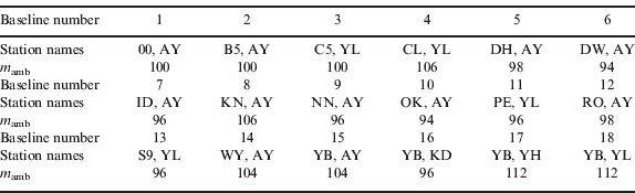
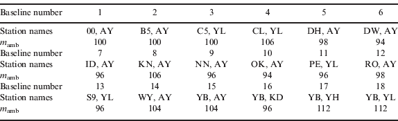
Table 1 lists the baseline number, the station names as well as the total number of ambiguities for each baseline in the network. The number of ambiguities per baseline is around 100, which is referred to as high dimension. The LAMBDA method was embedded into the “AMBRES” subroutine of the Bernese software package. The “RNX2SNX” processing control file (PCF) of Bernese was specified to compute the float ambiguity solution of each baseline. Then, both the LAMBDA and QIF methods in “AMBRES” are employed to fix the ambiguities, respectively. By comparing the fixed solutions derived from these two methods, the LAMBDA's performance is evaluated.
The station distribution and the formed baselines in the GPS network.

Baseline numbers, station names and the number of ambiguities (m amb) for each baseline in the network.
4.1. Numerical efficiency of LAMBDA
In this section, LAMBDA's performance in the ambiguity decorrelation and search is evaluated. The evaluation items include the precision of the ambiguity estimates, the decorrelation number, the search speed and the ambiguity spectrum before and after the decorrelation.
4.1.1. Precision of ambiguity estimates
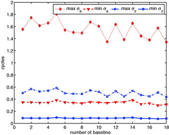
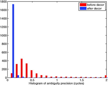
The ambiguity precisions (one sigma), σ a and σ z, calculated before and after the decorrelation are examined and the maximum and minimum ones for all 18 baselines are shown in Figure 2. Obviously, both the maximum and minimum precisions of the transformed ambiguities are much smaller. Figure 3 shows the histogram of total 1808 ambiguity precisions of the 18 baselines before and after the decorrelation. From this figure, it can be seen that before the decorrelation, the ambiguity precision is distributed over the interval from 0 to 2 cycles. After the decorrelation, the distribution interval is significantly reduced to smaller than 0·3 cycles, and most of the ambiguity precision is distributed over the smaller interval from 0 to 0·1 cycles. Therefore, the decorrelation has indeed succeeded in pushing the larger ambiguity precisions into much smaller values.
The maximum and minimum of the ambiguity precisions (one sigma) before and after the decorrelation.

Histogram of the ambiguity precisions (one sigma) of all the 18 baselines before and after the decorrelation.

4.1.2. Diagonality of variance-covariance matrix
The main purpose of the aforementioned decorrelation is to reduce the correlations amongst the ambiguities. Due to the integer constraints on the ambiguity transformation matrix Z, complete diagonality of the transformed ambiguity variance matrix can generally not be realised. We employ the decorrelation number, r, to measure the diagonality (correlation) degree of a matrix, which is defined as a ratio between the product of conditional standard deviations and the product of the standard deviations of this matrix. Thus the decorrelation number of the transformed variance-covariance matrix  is computed as:
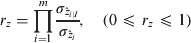
where  is the standard deviation of the ith ambiguity conditioned on the ambiguities from (i+1) to m;
 is the standard deviation of the ith ambiguity. The larger the r z is, the more diagonal the matrix is. Ideally, r z=1 which indicates a full decorrelation (diagonal matrix). For a geometrical interpretation on decorrelation number, one can refer to Teunissen et al (Reference Teunissen, de Jonge and Tiberius1996, Reference Teunissen, de Jonge and Tiberius1997).
To take the dimensional effect into account, we use the m-th root of r z in this paper
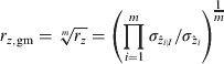
We have a similar formula to measure the diagonality of the original variance matrix  . According to the property, det(Z)=±1, of the decorrelating Z-transformation matrix, we have
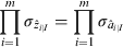
Thus, the decorrelation makes the variance matrix more diagonal, i.e., r z>ra or r z,gm>r a,gm, if  . The gain in decorrelation is defined as (Teunissen, Reference Teunissen1993)
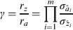
The large γ is associated to the high degree of the decorrelation. For the geometric interpretation of the decorrelation gain, one can refer to Teunissen (Reference Teunissen1993). Again considering the effect of the dimension, we use the m-th root of the decorrelation gain

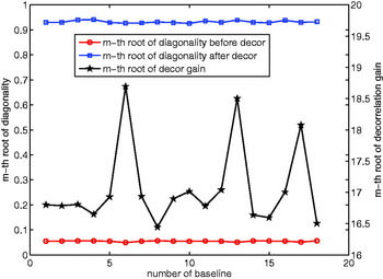
Figure 4 shows the m-th roots of the decorrelation number and the decorrelation gain for all baselines. It shows that the decorrelation indeed makes the ambiguity variance matrix much more diagonal. The m-th root of decorrelation number is improved from 0·055 to 0·932 on average for all the baselines after the decorrelation. Its corresponding m-th root of the decorrelation gain is as large as 17.
The m-th root of decorrelation number and the decorrelation gain before and after the decorrelation with m denoting the number of ambiguities of each baseline.

4.1.3. Spectrum of ambiguity conditional standard deviations
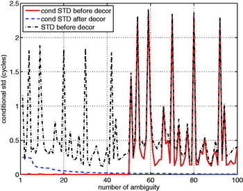
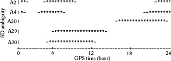
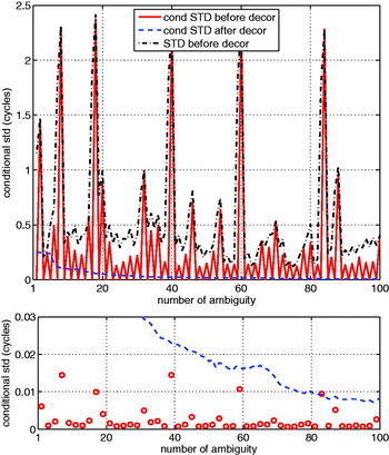
The purpose of the ambiguity decorrelation is not only to improve the ambiguity precision but also to flatten the spectrum of ambiguity conditional variances since the large discontinuities in the spectrum will result in the search halting, referring to De Jonge and Tiberius (Reference De Jonge and Tiberius1996). Figure 5 shows the spectrums of ambiguity conditional standard deviations before (red solid line) and after the decorrelation (blue dashed line) as well as the spectrum of ambiguity (unconditional) standard deviations before the decorrelation (black dash-dot line) for the first baseline. In this case, the ambiguity vector is structured as  . Understandably, the L1 ambiguity standard deviations have similar variation behaviour to the L2 ambiguity standard deviations. The spikes shown in Figure 5 are due to the poor observability of the corresponding ambiguities, i.e. they are linked to short observation time spans or poor observation quality. The part of the single-difference (SD) (between two receivers) satellite visibility plot output from Bernese is shown in Figure 6 for the first baseline. The asterisk indicates good quality observations during the corresponding 20 minute interval, while the dash marks the occurrence of missing epochs in the corresponding interval. The SD ambiguity A30 is selected as the reference to form DD ambiguities. The SD ambiguity A2 can form three DD ambiguities with A30 due to its discontinuity, and the first DD ambiguity has an extremely large standard deviation because of its short observation span. It is the same as the first DD ambiguity formed between A4 and A30. For more understanding of Figure 6 and more formation of the DD ambiguities in Bernese, one can refer to Dach et al (2007, p. 63 and p. 170).
The spectrum of ambiguity standard deviations before decorrelation and the spectrums of ambiguity conditional standard deviations before and after decorrelation for the first baseline.

SD (between-receiver) satellite visibility plot output from Bernese for the first baseline.

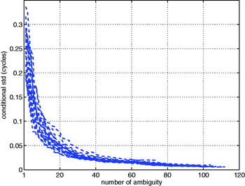
For the conditional standard deviations without decorrelation (red solid line) in the Figure 5, they have nosier and larger values in the second half part than in the first half part, and also a distinct jump exactly at the half-way of the spectrum. This is attributed to the high correlation between the L1 and L2 ambiguities and further to the presence of the ionospheric unknowns in the observation equations. After the decorrelation, the spectrum of conditional standard deviations (blue dashed line) is efficiently flattened; the spectrum jump vanishes and the magnitude of the spectrum is greatly reduced from 2·5 cycles to smaller than 0·3 cycles. The other 17 baselines in the network have the similar spectrums of conditional standard deviations without decorrelation to the first baseline in Figure 5. Their corresponding spectrums of the conditional standard deviations with decorrelation are illustrated in Figure 7, showing that the smooth spectrums have been realised.
To further examine the issue that L1 ambiguities are highly correlated with L2 ambiguities, we restructure the ambiguity vector 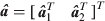 as:

where  and
 are the ith L1 and L2 ambiguities, respectively. For the restructured ambiguity vector
 of the first baseline, the spectrums of conditional standard deviations before and after decorrelation as well as the spectrum of (unconditional) standard deviations before decorrelation are plotted in Figure 8. The spikes also exist in both the conditional and unconditional standard deviations before decorrelation, which have the same attribution of poor observability as that in Figure 5. Now, we focus on examining the spectrum of the conditional standard deviations before decorrelation (read solid line). Considering the ambiguity order in , the elements in the upper subplot of Figure 8 from right to left are as follows. The first element is the unconditional standard deviation
 of
 , and the second is the conditional standard deviation
 of
 on the condition of . Analogously, the third element is the conditional standard deviation
 of
 on the condition of both and , and so on. Therefore, the figure has clearly shown (also see the bottom subplot of Figure 8) that L1 and L2 ambiguities from one ambiguity pair are highly correlated, while the ambiguities from the different ambiguity pairs are much less correlated.
The spectrums of ambiguity conditional standard deviations after decorrelation for all baselines in the network (each line for one baseline).

The spectrum of standard deviations before decorrelation and the spectrums of conditional standard deviations before and after decorrelation (upper subplot) as well as the conditional standard deviations of L1 ambiguities after decorrelation (bottom subplot) for the restructured ambiguity vector of the first baseline.

4.1.4. Numerical efficiency
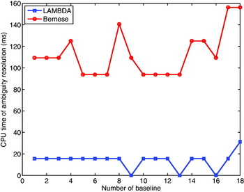
Up to now, the decorrelation has shown that it works well in the high-dimensional cases, i.e., after decorrelation, the ambiguity precision is improved, the variance-covariance matrix is more diagonal and the spectrum of conditional ambiguity standard deviations is flattened significantly. We further evaluate the computational efficiency of LAMBDA in comparison with Bernese. After the float ambiguities are solved, both the LAMBDA and QIF methods are used to fix the ambiguities. We record their consumed CPU time only in the ambiguity resolution processing for each baseline. The results are illustrated in Figure 9. LAMBDA turned out to be faster for all baselines since all of its results, except one, are less than 20 ms compared to about 100 ms using Bernese.
The consumed CPU time by LAMBDA and Bernese for the ambiguity resolution of each baseline.

4.2. Performance evaluation of LAMBDA
4.2.1. Performance evaluation in terms of fixed integers
To get an insight on how well LAMBDA works, we may directly compare its fixed integers with those of Bernese. It should be noted that the LAMBDA method fixes all ambiguities, while Bernese usually fixes only a subset of ambiguities and the fixed ambiguities are either the original DD ambiguities or the difference between two original ambiguities with the same reference SD ambiguity (actually, the newly formed DD ambiguities). We transform the fixed DD ambiguities from LAMBDA to the new ones that have the same combinations to those from Bernese. Assuming that the fixed integer ambiguity vector from LAMBDA is  , it is transformed by:

where Z is the transformation matrix from (10) and it is used to form the new ambiguities that to be fixed in Bernese;  is the transformed integer ambiguity vector, which has the same linear combination as the fixed ambiguity vector
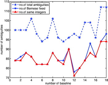
 from Bernese. Therefore, we can now directly compare with , and count the number of the same integer values. Figure 10 shows the number of fixed ambiguities by Bernese (i.e., the dimension of ), the number of same integers in both vectors and as well as the number of total ambiguities of each baseline. It is observed that, for most of baselines, the fixed ambiguities by Bernese can be also fixed by LAMBDA with the same integers. Furthermore, considering that some ambiguities fixed by LAMBDA cannot be fixed by Bernese, it is concluded that the fixed ambiguities by Bernese are generally the subset of the fixed ambiguities by LAMBDA.
The number of fixed ambiguities by Bernese (blue solid line with squares), the number of same integers in both vectors and (red solid line with triangles) as well as the number of total ambiguities of each baseline (blue dashed line with stars).

4.2.2. Performance evaluation in terms of baseline repeatability
From the test results of the previous section, one cannot judge whether the ambiguities fixed by both methods are correct or not. Therefore, we further evaluate the LAMBDA performance by analysing the effect of its integer solutions on the baseline repeatability (i.e., empirical baseline precision) in this section. From now on, we use a total of 12-day dual-frequency GPS data from the same network in Figure 1. We design different experiment scenarios by specifying the observation spans of 2, 3, 4, 6, 12 and 24 hours, respectively. If the session span is 6 hours, the total number of sessions for 12 days is 24/6×12=48, which means that we can obtain 48 fixed solutions for each baseline.
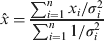
The baseline repeatability is defined as:
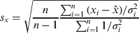
where n is the number of sessions from which the baseline was solved for; x i and σ i are the baseline component estimate and its standard deviation from the ith session, respectively;  is the weighted mean of the baseline component and calculated based on the component estimates of all sessions:
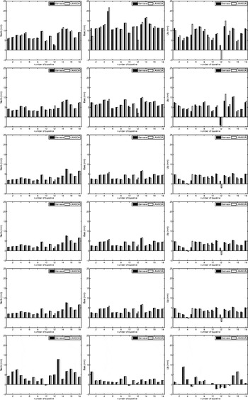
According to (20), one can compute the baseline repeatabilities with both the float and fixed ambiguities, say, s float and s fix. Figure 11 shows the comparison of baseline repeatability between the float solution and the fixed solution of LAMBDA as well as the fixed solution of Bernese, namely:

A positive Δs value means that the precision of the fixed solution is higher than that of the float solution. In Figure 11, the results from the first row to the last row are for the observation spans of 2, 3, 4, 6, 12 and 24 hours respectively, and from left to right the columns are for the north, east and up components. From all subplots, it can be seen that most of the Δs values are positive, which means that the baseline repeatability of the fixed solution is much better than that of the float solution. In addition, with the observation span getting longer, the baseline repeatability difference between the float solution and the fixed solution becomes smaller. It makes sense, because the baseline estimates solved from a long observation span have high precision even using the float ambiguity. It is also observed that the horizontal components (especially the east component in the second column of Figure 11) have significant improvements for all observation spans, while the up component has a moderate improvement and, for some baselines, degrades after ambiguity fixing although the degradation is very small. Such results are consistent with those reported by Blewitt (Reference Blewitt1989) and Ge et al (Reference Ge, Gendt, Rothacher, Shi and Liu2008).
The difference between the baseline repeatabilities with the fixed ambiguities from LAMBDA and Bernese is also calculated

where s ber and s lmd are the baseline repeatabilities with the fixed ambiguities from Bernese and LAMBDA, respectively. A positive Δs indicates that the precision of the baseline component with the fixed ambiguities from LAMBDA is higher than that from Bernese. As shown in Figure 12, for the short observation spans, it seems that LAMBDA is marginally better than Bernese in the up component. For the 2-hour observation span, the baseline repeatability differences, i.e. the Δs values, are within several millimetres. Also with the observation span getting longer, the differences become smaller. The differences are smaller than 1 mm for all the baselines when the observation span is longer than 12 hours. Such small difference can be adequately ignored in practice. Therefore, the baseline repeatabilities derived from LAMBDA and Bernese can be considered comparable for practical purposes.
The difference of baseline repeatability computed using the float ambiguity estimates and the fixed ambiguity estimates derived from LAMBDA and Bernese. The results from the first row to the last row are for the observation spans of 2, 3, 4, 6, 12 and 24 hours, and from left to right for north, east and up components, respectively.

The difference of baseline repeatabilities computed using the fixed ambiguities from Bernese and LAMBDA. The results from left to right and up to bottom are for the observation spans of 2, 3, 4, 6, 12 and 24 hours respectively.

4.2.3. Baseline repeatability with the ambiguity resolved from a network
In the Bernese software, one could solve for the float ambiguities of all baselines in a network depending on the size of network and observation span etc, but the ambiguity fixing processing is performed only in baseline-by-baseline mode. It is feasible to use LAMBDA to fix all ambiguities from this network simultaneously. In Bernese, the number of unknown parameters is limited for the purpose of computation efficiency. Thus it is advised to use the baseline mode to solve float ambiguities instead of using the network mode, unless the network is small, e.g. it only consists of several baselines along with sufficiently short observation spans. In our experiment, a total of 18 baselines are tested and thus we can only solve the network float ambiguities with observation span of 2 hours. Otherwise, the number of parameters will exceed the parameter threshold. In the network solution, the number of ambiguity parameters generally exceeds 400. First of all, we address whether the LAMBDA method works still efficiently in the network mode. Using the 12-day data the same as that used in the subsection 4.2.2, the total number of the sessions is 24/2×12=144, which means that there are 144 network ambiguity solutions. The spectrum of ambiguity conditional standard deviations from the network ambiguity solution mode is very noisy before decorrelation and with magnitude of 2·5 cycles although they are not illustrated here. After the decorrelation, these values are all smaller than 0·3 cycles as shown in Figure 13. This indicates that the decorrelation is still efficient in the high dimensional case even with more than 400 ambiguities.
The spectrum of the ambiguity conditional standard deviations from all the 144 network ambiguity solutions after the decorrelation (each line for one network solution).

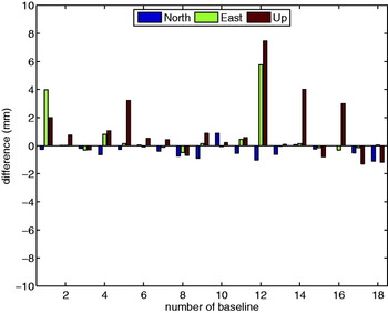
We can also employ LAMBDA to fix the ambiguities of the network solutions and then compute the baseline component estimates as well as the baseline repeatability s network. Let the baseline repeatability using the ambiguity resolved from the baseline-by-baseline mode be s baseline, the difference between the two baseline repeatabilities are calculated by:

A positive Δs value means that the baseline repeatability from the network mode is better than that from the baseline-by-baseline mode. It is observed from Figure 14 that, for most of the baselines, the results from the two ambiguity resolution modes are similar, whereas for the 1st and 12th baselines, the Δs values reach 4 mm and 8 mm. The reason is that these two baselines have poor baseline repeatabilities with baseline-by-baseline mode, see the first subplot of Figure 12. Therefore, it is concluded that for the baselines that have good baseline repeatabilities from the baseline-by-baseline mode, the comparable baseline repeatabilities are achievable from the network mode. However, for the baselines with poor baseline repeatabilities from the baseline-by-baseline mode, they may be further improved by the network mode. It is emphasised again that the network ambiguity fixing mode is not available in Bernese software.
The difference of the baseline repeatabilities based on the fixed ambiguities resolved from LAMBDA using the baseline-by-baseline and the network modes, respectively; GPS data session is 2 hours.

5. CONCLUDING REMARKS
The LAMBDA method has been widely used for carrier phase ambiguity resolution with the number of ambiguities up to several tens in the past two decades. With the advent of denser network and the availability of multi-frequency, multi-GNSS systems, it is significant to understand LAMBDA's efficiency and performance in high dimensional ambiguity spaces.
In this contribution, a first attempt was made to analyse the LAMBDA performance in high-dimensional ambiguity spaces using the real GPS data. We have embedded the LAMBDA method into the Bernese software for evaluating and comparing its performance with Bernese approach. The performance evaluation includes the numerical efficiency of the decorrelation and search steps of LAMBDA itself, and the effect of the LAMBDA optimal integer solution on the baseline precision. The experiment results suggest that the LAMBDA method is still efficient in high dimensional ambiguity spaces. The results of the LAMBDA's performance in terms of the baseline repeatability suggest that the baseline repeatability resulted from the LAMBDA solution are comparable with those from Bernese. However, if the baseline precision obtained from the baseline-by-baseline ambiguity resolution mode is poor, one can further improve it by using the network ambiguity resolution mode based on LAMBDA. Therefore, for future denser network processing and multi-GNSS tracking, the easy-to-use LAMBDA method should be considered as an alternative to those approaches used in some prestigious software packages, such as Bernese.Footnote 1
We note that a further improvement is possible in our analyses, since (i) we used the LAMBDA method only as a full ambiguity resolver (i.e. no partial ambiguity resolution was attempted) and (ii) the fixed ambiguities in this paper were not independently validated, e.g. the fixed failure-rate ratio test was not performed.
ACKNOWLEDGMENTS
This work has been conducted in the context of the Positioning Program of the Cooperative Research Centre Spatial Information (CRC-SI). The second author is the recipient of an Australian Research Council (ARC) Federation Fellowship (Project No.: FF0883188). This support is gratefully acknowledged.