1. Introduction
There has been an increasing interest in developing cooperative robotic systems as reliable solutions to different demands during the last decades. Cooperative robotic systems comprise robots that work together as a team to complete a common task. Examples of these systems include cooperative UAVs, mobile robots, and manipulators [Reference Gimenez, Gandolfo, Salinas, Rosales and Carelli1–Reference Qian, Zi and Ding3]. The importance of these systems has led to the emergence of various control methods for them. One of the usual strategies of controlling cooperative robots is the model-based approach [Reference AzizZadeh, Menhaj and Talebi4–Reference Pizetta, Brandão and Sarcinelli-Filho7].
Despite some benefits, model-based controllers are developed based on the accurate modeling of systems. However, dynamic equations of systems are usually obtained using approximations or simplifications. As a result, uncertainties appear in the system model, which challenges the model-based controller design and makes them unreliable. On the contrary, the model-free techniques can reject the model imprecisions by choosing data-driven approaches [Reference Chen and Lin8].
To this mean, many researchers have developed adaptive methods for cooperative robotic systems. In ref. [Reference Pliego-Jimenez and Arteaga-Perez9], an adaptive force-position controller is designed using time-varying constraints for two robotic arms handling an object. Reference [Reference Marino10] has introduced a two-layer observer-control structure for mobile manipulators that handle an object. An adaption law is also developed in this research to address the issue of uncertainty. In ref. [Reference Sun, Huo and Jiao11], the relative orientation and position are controlled for a cooperative spacecraft system. An adaptive rule is presented to deal with uncertainties, and the stability of the whole system is confirmed. In ref. [Reference Shojaei12], an adaptive and robust controller is presented for a robotic system based on the PID concept. The stability is proved using the Lyapunov lemma. An adaptive controller for multiple quadrotors carrying a load together is developed in ref. [Reference Arab, Shirazi and Yazdi13]. The Lyapunov theorem is used to verify the system’s stability. Other robust methods are also developed to confront disturbances and uncertainties. In ref. [Reference Yang, Zong, Nguang and Zhao14], a disturbance observer-based bumpless transfer H∞ control scheme is developed for switching Markovian LPV systems. Reference [Reference Zong, Li and Sun15] presents a robust disturbance observer-based controller for Markovian systems. It is proved that the system is stable according to the exact Lyapunov analysis. In ref. [Reference Zong, Ren and Karimi16], the issue of confronting disturbances is investigated by proposing a finite-time H∞ filter for networked switched systems.
Besides, various neural network or fuzzy-based controllers are released to confront the uncertainties and disturbances and control the robotic systems effectively. In ref. [Reference Baigzadehnoe, Rahmani, Khosravi and Rezaie17], an adaptive fuzzy backstepping-based approach is proposed for cooperative manipulators that move an object. The suggested controller confirms that the system is uniformly ultimately bounded (UUB). Hu et al. modeled cooperative robotic arms based on a Markovian switching network and used the neural network framework as an adaptive controller. Uniform exponential stability of the system is assured theoretically [Reference Hu, Guan, Lewis and Chen18]. In ref. [Reference Thusoo, Jain and Bangia19], a hybrid neuro-fuzzy control approach is presented to settle the problem of path tracking for collaborating UAVs. The Kalman filter is utilized to distinguish the obstacle position and avoid collisions. In ref. [Reference Khan, Li and Cao20], a zeroing neural network is utilized for cooperative trajectory tracking of mobile arms. A Metaheuristic approach is utilized to optimize the controller. Reference [Reference Wu, Jin, Liu and Yu21] dealt with the tracking problem of cooperative manipulators by presenting a predictive control scheme based on neural networks. The uncertainties are regarded as the disturbance in this research, and an extended observer is designed to attenuate its effect. The issue of handling an object by cooperative robots is addressed in ref. [Reference Farahmandrad, Ganjefar, Talebi and Bayati22] by proposing a fuzzy sliding mode controller. To this mean, the cooperative system dynamics is decomposed using the passive decomposition method. In ref. [Reference Zong, Sun and Nguang23], systems with strong interconnections are efficiently controlled by proposing an adaptive neuro-feedback controller. A decentralized observer is also developed to approximate the unknown states. In ref. [Reference Li, Yang, Yan, Cui, Annamalai, Netw and Syst24], first, an admittance model is developed for a cooperative system comprised of robotic arms that transport a common object. Then, the uncertainties are approximated using an adaptive neural network. Reference [Reference Yu, Zhang, Jiang, Su, Fu, Jin and Chai25] proposes a fractional-order PID control approach to handle the path tracking problem of a team of networked aerial vehicles. The recurrent neural network is employed in this study to approximate the wind disturbance and actuator defects.
One of the problems with many proposed controllers is the need to measure states, especially velocities. While in many dynamic systems, especially commercial robots, it is not possible to measure speed, and the position can only be measured. The reason for not measuring speed is that using a sensor for this mean is not economically viable. On the other hand, noise interference when measuring states causes a decrease in bandwidth [Reference Ortega, Perez, Nicklasson and Sira-Ramirez26]. In ref. [Reference Shojaei27], a neural adaptive PID controller is designed for mobile robots. The designed controller does not depend on velocity measurements. In many control methods, the system velocities are obtained by using position differentiation, which is not a good solution because it causes chattering in the signals. Designing a state observer is an effective technique to address this issue. In ref. [Reference Zhang, Song and Zhao28], a payload is moved by multi-manipulators, and it is assumed that the velocities are not measured. So, velocities are approximated by proposing an observer. Then, the cooperative system is controlled using a neuro-adaptive approach. Li et al. studied the issue of load-carrying by several robotic arms [Reference Li, Xu, Li, Wu and Zhou29]. An observer is proposed for the system to approximate the velocities, and the system is controlled using recurrent neural networks.
The important issue is that, even though neural networks and fuzzy systems can estimate different functions due to the universal approximation property [Reference Izadbakhsh, Zamani and Khorashadizadeh30–Reference Izadbakhsh, Khorashadizadeh and Kheirkhahan32], they have problems that make their design and implementation challenging. In fuzzy observer/controller design, it is necessary to determine factors such as the type of membership functions, their number and range, fuzzification and defuzzification methods, the database of rules, and the fuzzy inference system. In neural networks, on the other hand, it is required to define the network type, the number of hidden layers and neurons, and the activation functions type. Determining all these parameters requires sufficient design knowledge and experience, and also, their complex structure makes it difficult to apply them, raising the computational complexity of the control system [Reference Izadbakhsh33, Reference Izadbakhsh and Khorashadizadeh34].
The function approximation technique (FAT) is a relatively new method for approximating diverse functions such as uncertainties. Various approaches based on the FAT have been formed, such as Legendre polynomials [Reference Zarei and Khorashadizadeh35], differential equations [Reference Izadbakhsh and Nikdel36, Reference Izadbakhsh and Khorashadizadeh37], and Fourier series [Reference Kheirkhahan and Izadbakhsh38, Reference Deylami and Izadbakhsh39], and Bernstein–Stancu operator [Reference Izadbakhsh and Nikdel40]. Simple structures of FATs in comparison with neural or fuzzy-based methods made them ideal candidates for function approximation [Reference Izadbakhsh, Khorashadizadeh and Ghandali41–Reference Izadbakhsh, Akbarzadeh Kalat and Khorashadizadeh43].
In this paper, cooperating manipulators are considered to be in charge of moving an object. The object should track the desired path, and the force applied to it should be controlled. The major advantages of FAT-based methods compared to both model-free neuro-fuzzy and model-based approaches, which make them suitable choices for coping with uncertainties and disturbances, are the motivation for using them to construct the structure. The following are the most essential advantages: (1) Changes in parameters of model-based controllers can have a significant impact on system performance. FAT-based strategies, in contrast to these approaches, are not reliant on system modeling. As a result, the presence of unmodeled dynamics does not affect their performance; (2) the parameters of the approximator/controller must be determined with adequate skill when designing systems using neural networks or fuzzy logic. Lack of adequate expertise will change the design process into a time-consuming task because it is essential to adjust the parameters based on trial and error. On the other hand, the values of parameters in FAT-based techniques are easily established due to the low number of factors and the uncomplicated structure; (3) projection methods are commonly required in neuro-fuzzy systems to maintain the parameters in a specific range, which adds to the controller’s computing load; (4) different state feedbacks are frequently required by neuro-fuzzy designs. As an instance, the neuro-fuzzy estimator requires the system states as inputs if the uncertainty is a function of them, increasing the system’s computational load. On the other hand, FAT-based approximators estimate functions as time series and are not affected by states. This process reduces the computational complexity of the system [Reference Izadbakhsh33, Reference Izadbakhsh and Khorashadizadeh44]. The chief properties of function approximation techniques, fuzzy methods, and neural networks are compared in Table I.
A comparison among FATs, fuzzy methods, and neural networks.

The FAT is utilized in this study to confront disturbances and unmodulated dynamics, ensuring that their impact does not degrade system efficiency. Bernstein-type operators (BTO) are utilized to approximate disturbances and uncertainties, and the polynomial coefficients are adjusted through adaptive laws development. The Lyapunov theorem is used to confirm the boundedness of all error signals during the stability analysis. Finally, two 3-degree-of-freedom (DOF) robotic arms carrying a payload are used to test the efficacy of the presented adaptive FAT-based technique. The following are the proposed approach’s novelty and benefits: (1) To the authors’ knowledge, this is the first application of Bernstein-type operators for estimating continuous functions on the semi-axis in designing a robust adaptive controller for electrically driven cooperating multi arms; (2) the proposed control method is regressor-free. As a result, the suggested controller avoids the drawbacks of traditional adaptive approaches; (3) one of the benefits of the proposed approach is that joint speed is not monitored, and the only measured state is position; (4) furthermore, the joint torque is considered as the control input in the majority of previously established methods, and actuator dynamics are ignored. However, actuator voltages are treated as control signals in this study as a more reasonable assumption.
Different sections of the article are as follows: The Bernstein-type operators are described in Section 2. Section 3 reveals the dynamic model of the coordinated robotic arms. Section 4 explains the design steps of the adaptive controller-observer, as well as the rigorous stability analysis. The simulation results are illustrated in Section 5, and the most relevant concluding points are presented in Section 6. Though this paper,
 $\underline{\lambda}(\!\boldsymbol\cdot\!)$
denotes the minimum eigenvalue of a bounded positive-definite matrix
 $(\!\boldsymbol\cdot\!)$
, and
 $\overline{\lambda}(\!\boldsymbol\cdot\!)$
is the corresponding maximum eigenvalue. Suppose a vector
 ${\bf{y}} \in {\Re ^n}$
, its norm is indicated as
 $\left\| {\bf{y}} \right\| = \sqrt {{{\bf{y}}^T}{\bf{y}}} $
, and the norm of the matrix
 ${\bf{{E}}}$
is calculated as
 $\left\| {{\bf{{E}}}(y)} \right\| = \sqrt {\bar \lambda ({\bf{{E}}}{{(y)}^T}{\bf{{E}}}(y))} $
.
2. Bernstein-Type Operators Approximating Continuous Functions on the Semi Axis
The use of positive linear operators as approximators has been a popular topic. This section aims to describe the Bernstein-type operator
 ${L_n}$
that is defined by a finite sum on
 $C[0,\infty )$
, which stands for the continuous functions space on the interval
 $[0,\infty )$
. The operator
 ${L_n}:C[0,\infty )$
is described as follows [Reference Bleimann, Butzer and Hahn45].
 \begin{align} ({L_{{\rm{}}\Xi }}g)(t) = {(1 + t)^{ - \Xi }}\sum\limits_{k = 0}^\Xi g \left( {{k \over {\Xi - k + 1}}} \right)\left( \begin{matrix} \Xi \\[4pt] k \end{matrix} \right){t^k},\,\,\,(\Xi \in {\rm{N}})\end{align}
According to Theorem 1 from ref. [Reference Bleimann, Butzer and Hahn45], if
 $g$
is continuous on
 $[0,\infty )$
, then
 \begin{align} \mathop {\lim }\limits_{\Xi \to \infty } ({L_\Xi }g)(t) = g(t)\end{align}
at each point
 $t \in [0,\infty )$
, the convergence being uniform on each compact subinterval
 $[0,b)$
of
 $[0,\infty )$
.
3. Dynamic Model of Coordinated Robotic Systems
3.1. System overview and assumptions
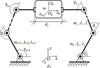
A typical object is considered to be handled by m actuated robotic arms, which have n degrees of freedom (DOF), in the workspace. Different coordinate frames are placed to model the system, as shown in Fig. 1. The end-effector and object positions, and their orientations, are referred to in the
 $\textrm{OXYZ}$
base frame. The coordinate frame of the object, defined as
 ${{\rm O}_{\rm o}}{{\rm X}_{\rm o}}{{\rm Y}_{\rm o}}{{\rm Z}_{\rm o}}$
, is placed at its center of mass (COM). For ith manipulator, the coordinate frame
 ${{\rm O}_{\rm ei}}{{\rm X}_{\rm ei}}{{\rm Y}_{\rm ei}}{{\rm Z}_{\rm ei}}$
is considered at its grasp point.
The Coordinate robotic system.

The subsequent assumptions are presumed to develop the dynamic model of the system [Reference Jean, Fu and Automat46, Reference Song and Cai47].
Assumption 1: All of the manipulators are non-redundant, which means that the workspace dimension and each robot DOF are equal.
Assumption 2: The rigid attachment of all end-effectors and the common object resulted in zero relative movements between them.
Assumption 3: Each robot’s kinematics are precisely known. Moreover, each manipulator avoids kinematics singularities while moving. This indicates that each robot’s Jacobian matrix is full-rank and known.
Assumption 4: The object is considered to be rigid, which means that applying forces does not result in its distortion.
3.2. Actuators dynamic model
The rotational behavior of n DC motors operating an n-degree-of-freedom robot is described by the following differential equations [Reference Spong and Vidyasagar48].
 \begin{align} {{\bf{J}}_{ai}}{\boldsymbol{\ddot{ \unicode{x1D6B9} }}_i} + ({{\bf{b}}_{ai}} + {{\bf{k}}_{ai}}{{\bf{k}}_{bi}}{\bf{R}}_i^{ - 1}){\boldsymbol{\dot{ \unicode{x1D6B9} }}_i} = {{\bf{k}}_{ai}}{\bf{R}}_i^{ - 1}{{\bf{v}}_i}(t) - {{\bf{r}}_i}{{\boldsymbol{\unicode{x1D6BB} }}_{li}}{\rm{, }}\quad i{\rm{ = 1,2,}} \ldots {\rm{,}}m\end{align}
where
 ${{\boldsymbol{\unicode{x1D6B9} }}_i} \in {\Re ^n}$
is the actuator angle vector,
 ${{\bf{J}}_{ai}} \in {\Re ^{n \times n}}[kg.{m^2}]$
is a diagonal matrix consisting of the actuator side elements of the transmission and the lumped rotor inertias,
 ${{\bf{b}}_{ai}} \in {\Re ^{n \times n}}[N.m.s/rad]$
is the diagonal matrix of actuator side elements of the transmission and the lumped motor damping coefficients,
 ${{\bf{k}}_{ai}} \in {\Re ^{n \times n}}[N.m/A]$
and
 ${{\bf{k}}_{bi}} \in {\Re ^{n \times n}}[N.m/A]$
are the diagonal matrices of motor-torque, and the back EMF constants, respectively.
 ${{\bf{R}}_i} \in {\Re ^{n \times n}}[\Omega ]$
is diagonal matrix of armature resistances,
 ${{\bf{v}}_i}(t) \in {\Re ^n}[v]$
is the armature voltages vector,
 ${{\boldsymbol{\unicode{x1D6BB} }}_{li}} \in {\Re ^n}[N.m]$
is the load torques vector, and
 ${{\bf{r}}_i}$
is an n×n transmission matrix, which maps the n×1 motor coordinate speeds vector,
 ${\boldsymbol{\dot{ \unicode{x1D6B9} }}_i}$
, into the generalized joint coordinate speeds vector,
 ${{\dot{\bf q}}_i}$
, as
 \begin{align} {{\dot{\bf q}}_i} = {{\bf{r}}_i}{\boldsymbol{\dot{ \unicode{x1D6B9} }}_i}{\rm{, }}\quad i{\rm{ = 1,2,}} \ldots {\rm{,}}m\end{align}
Remark 1: Equation (3) has been obtained under the assumption that the electrical time constant is smaller than the mechanical time constant.
3.3. Manipulators dynamic model
In the joint space, the ith manipulator dynamic model is formulated as [Reference Spong and Vidyasagar48, Reference Izadbakhsh, Akbarzadeh Kalat, Fateh and Rafiei49],
 \begin{align} {{\bf{D}}_i}({{\bf{q}}_i}){{\ddot{\bf q}}_i} + {{\bf{C}}_i}({{\bf{q}}_i},{{\dot{\bf q}}_i}){{\dot{\bf q}}_i} + {{\bf{G}}_i}({{\bf{q}}_i}) = {{\boldsymbol{\unicode{x1D6BB} }}_{li}} - {\bf{J}}_{ei}^T({{\bf{q}}_i}){{\bf{F}}_{ei}} {\rm{, \quad i = 1,2,}} \ldots {\rm{,m}}\end{align}
where the vector
 ${{\bf{q}}_i} \in {\Re ^n}$
indicates the joint variables.
 ${{\bf{D}}_i}({{\bf{q}}_i}) \in {\Re ^{n \times n}}$
is the positive-definite and symmetric inertia matrix. The matrix of centrifugal/Coriolis is represented by
 ${{\bf{C}}_i}({{\bf{q}}_i},{{\dot{\bf q}}_i}) \in {\Re ^{n \times n}}$
. The gravitational force vector is shown by
 ${{\bf{G}}_i}({{\bf{q}}_i}) \in {\Re ^n}$
, and the Jacobian matrix is
 ${{\bf{J}}_{ei}}({{\bf{q}}_i}) \in {\Re ^{n \times n}}$
. At the grasp point, the ith manipulator end-effector exerts a force on the common object, which is presented by
 ${{\bf{F}}_{ei}} \in {\Re ^n}$
.
Concise representation of m manipulators dynamics actuated by DC motors (3) is
 \begin{align} {\bar{\bf D}}({\bf{q}}){\ddot{\bf q}} + {\bar{\bf C}}({\bf{q}},{\dot{\bf q}}){\dot{\bf q}} + {\bf{G}}({\bf{q}}) = {{\bf{r}}^{ - 1}}{{\bf{k}}_a}{{\bf{R}}^{ - 1}}{\bf{v}} - {\bf{J}}_e^T({\bf{q}}){{\bf{F}}_e}\end{align}
that
 \begin{align} {\bf{q}} & = {\left[ {{{\bf{q}}_1^T}{{\bf{q}}_2^T} \ldots {{\bf{q}}_m^T}} \right]^T} \in {\Re ^{mn}} \nonumber \\[5pt] {\bf{v}} & = {\left[ {{{\bf{v}}_1^T}{{\bf{v}}_2^T} \ldots {{\bf{v}}_m^T}} \right]^T} \in {\Re ^{mn}} \nonumber \\[5pt] {\bar{\bf D}}({\bf{q}}) &= blockdiag\left[ {{{{\bf{D}}_1}({{\bf{q}}_1}) + {\bf{r}}_1^{ - 1}{{\bf{J}}_{a1}}{\bf{r}}_1^{ - 1}}{{{\bf{D}}_2}({{\bf{q}}_2}) + {\bf{r}}_2^{ - 1}{{\bf{J}}_{a2}}{\bf{r}}_2^{ - 1}} \ldots {{{\bf{D}}_m}({{\bf{q}}_m}) + {\bf{r}}_m^{ - 1}{{\bf{J}}_{am}}{\bf{r}}_m^{ - 1}}} \right] \in {\Re ^{mn \times mn}} \nonumber \\[5pt] {\bar{\bf C}}({\bf{q}},{\dot{\bf q}}) & = blockdiag\left[ {{{{\bf{C}}_1}({{\bf{q}}_1},{{{\dot{\bf q}}}_1}) + {\bf{r}}_1^{ - 1}({{\bf{b}}_{a1}} + {{\bf{k}}_{a1}}{{\bf{k}}_{b1}}{\bf{R}}_1^{ - 1}){\bf{r}}_1^{ - 1}} \ldots } \right. \nonumber \\[5pt] & \quad\qquad\qquad \; {\rm{ }}\left. {{{\bf{C}}_m}({{\bf{q}}_m},{{{\dot{\bf q}}}_m}) + {\bf{r}}_m^{ - 1}({{\bf{b}}_{am}} + {{\bf{k}}_{am}}{{\bf{k}}_{bm}}{\bf{R}}_m^{ - 1}){\bf{r}}_m^{ - 1}} \right] \in {\Re ^{mn \times mn}}\nonumber\\[5pt] {\bf{G}}({\bf{q}}) & = {\left[ {{{{\bf{G}}_1}({{\bf{q}}_1})}\;\;\;\;{{{\bf{G}}_2}({{\bf{q}}_2})} \ldots {{{\bf{G}}_m}({{\bf{q}}_m})}} \right]^T} \in {\Re ^{mn}} \\[5pt] {{\bf{r}}^{ - 1}}{{\bf{k}}_a}{{\bf{R}}^{ - 1}} & = blockdiag\left[ {{{\bf{r}}_1^{ - 1}{{\bf{k}}_{a1}}{\bf{R}}_1^{ - 1}}\;\;\;\;{{\bf{r}}_2^{ - 1}{{\bf{k}}_{a2}}{\bf{R}}_2^{ - 1}} \ldots {{\bf{r}}_m^{ - 1}{{\bf{k}}_{am}}{\bf{R}}_m^{ - 1}}} \right] \in {\Re ^{mn \times mn}} \nonumber \\[5pt] {{\bf{J}}_e}({\bf{q}}) & = blockdiag\left[ {{{\bf{J}}_{e1}^T({{\bf{q}}_1})}\;\;\;\;{{\bf{J}}_{e2}^T({{\bf{q}}_2})} \ldots {{\bf{J}}_{em}^T({{\bf{q}}_m})}} \right] \in {\Re ^{mn \times mn}} \nonumber \\[5pt] {{\bf{F}}_e} & = {\left[ {{{\bf{F}}_{e1}^T}\;\;\;\;{{\bf{F}}_{e2}^T} \ldots {{\bf{F}}_{em}^T}} \right]^T} \in {\Re ^{mn}} \nonumber \end{align}
3.4. Dynamic model of the object
The object motion is formulated as [Reference Jean, Fu and Automat46, Reference Yao and Tomizuka50],
 \begin{align} {{\bf{D}}_o}({{\bf{x}}_o}){{\ddot{\bf x}}_o} + {{\bf{C}}_o}({{\bf{x}}_o},{{\dot{\bf x}}_o}){{\dot{\bf x}}_o} + {{\bf{G}}_o}({{\bf{x}}_o}) = {{\bf{F}}_o}\end{align}
In this equation,
 ${{\bf{x}}_o} \in {\Re ^n}$
denotes the object frame (
 ${{\rm O}_{\rm o}}{{\rm X}_{\rm o}}{{\rm Y}_{\rm o}}{{\rm Z}_{\rm o}}$
) position vector, as well as its orientation vector, relative to the base frame (
 ${\rm OXYZ}$
). The object inertial matrix, which is positive definite, and symmetric is represented by
 ${{\bf{D}}_o}({{\bf{x}}_o}) \in {\Re ^{n \times n}}$
. The Coriolis/centrifugal matrix is shown by
 ${{\bf{C}}_o}({{\bf{x}}_o},{{\dot{\bf x}}_o}) \in {\Re ^{n \times n}}$
.
 ${{\bf{G}}_o}({{\bf{x}}_o}) \in {\Re ^n}$
shows the gravitational vector, and the force exerted on the object’s center of mass is presented by
 ${{\bf{F}}_o} \in {\Re ^n}$
.
Consider
 ${{\bf{J}}_o}({{\bf{x}}_o}) \in {\Re ^{mn \times n}}$
to be defined as
 \begin{align} {{\bf{J}}_o}({{\bf{x}}_o}) = {\left[ {\begin{array}{*{20}{c}}{{\bf{J}}_{o1}^T({{\bf{x}}_o})}\;\;\;\;\;{{\bf{J}}_{o2}^T({{\bf{x}}_o})}\;\;\;\;\; \ldots\;\;\;\;\; {{\bf{J}}_{om}^T({{\bf{x}}_o})}\end{array}} \right]^T}\end{align}
where
 ${{\bf{J}}_{oi}}({{\bf{x}}_o}) \in {\Re ^{n \times n}}$
stands for the object frame (
 ${{\rm O}_{\rm o}}{{\rm X}_{\rm o}}{{\rm Y}_{\rm o}}{{\rm Z}_{\rm o}}$
) Jacobian matrix relative to the ith robot end-effector frame (
 ${{\rm O}_{\rm ei}}{{\rm X}_{\rm ei}}{{\rm Y}_{\rm ei}}{{\rm Z}_{\rm ei}}$
). Therefore,
 ${{\bf{F}}_o}$
is obtained
 \begin{align} {{\bf{F}}_o} = {\bf{J}}_o^T({{\bf{x}}_o}){{\bf{F}}_e}\end{align}
When the consequent force
 ${{\bf{F}}_o}$
is known, the end-effector force
 ${{\bf{F}}_e}$
, which fulfils (10), is decomposable into two orthogonal parts corresponding to the object movement and the internal force production. Eq. (11) represents this decomposition [Reference Jean, Fu and Automat46, Reference Song and Cai47].
 \begin{align} {{\bf{F}}_e} = {({\bf{J}}_o^T({{\bf{x}}_o}))^ + }{{\bf{F}}_o} + {{\bf{F}}_I}\end{align}
where
 ${({\bf{J}}_o^T({{\bf{x}}_o}))^ + } = {{\bf{J}}_o}({{\bf{x}}_o}){({\bf{J}}_o^T({{\bf{x}}_o}){{\bf{J}}_o}({{\bf{x}}_o}))^{ - 1}} \in {\Re ^{mn \times n}}$
represents the pseudo-inverse of
 ${\bf{J}}_o^T({{\bf{x}}_o})$
, and the internal force vector is represented by
 ${{\bf{F}}_I} \in {\Re ^{mn}}$
which is defined in the
 ${\bf{J}}_o^T({{\bf{x}}_o})$
null space, which means that it satisfies
 \begin{align} {\bf{J}}_o^T({{\bf{x}}_o}){{\bf{F}}_I} = 0\end{align}
Combining (8) and (11) results in
 \begin{align} {{\bf{F}}_e} = {({\bf{J}}_o^T({{\bf{x}}_o}))^ + }\left( {{{\bf{D}}_o}({{\bf{x}}_o}){{{\ddot{\bf x}}}_o} + {{\bf{C}}_o}({{\bf{x}}_o},{{{\dot{\bf x}}}_o}){{{\dot{\bf x}}}_o} + {{\bf{G}}_o}({{\bf{x}}_o})} \right) + {{\bf{F}}_I}\end{align}
3.5. Combined whole system dynamics
The total number of position variables introduced in (6) and (8) is equal to (m+1)n; n of which are independent. The reason is that for a known object trajectory, each manipulator joint trajectory is uniquely specified based upon Assumptions 1 and 2. Equations (6) and (8) are not appropriate for analyzing system dynamics due to position variables dependence. So, the dynamic model (6), which explains the behavior of the overall system, can be formulated using the object position
 ${{\bf{x}}_o}$
because of its independence.
Let
 ${{\bf{x}}_{ei}} \in {\Re ^n}$
indicate the vector of the position/orientation related to the ith end-effector. Then, the relation between
 ${{\dot{\bf x}}_{ei}}$
and
 ${{\dot{\bf q}}_i}$
is established by the Jacobian matrix
 ${{\bf{J}}_{ei}}({{\bf{q}}_i})$
as follows.
 \begin{align} {{\dot{\bf x}}_{ei}} = {{\bf{J}}_{ei}}({{\bf{q}}_i}){{\dot{\bf q}}_i}\end{align}
and
 ${{\dot{\bf x}}_{ei}}$
is related to
 ${{\dot{\bf x}}_o}$
as follows.
 \begin{align} {{\dot{\bf x}}_{ei}} = {{\bf{J}}_{oi}}({{\bf{x}}_o}){{\dot{\bf x}}_o}\end{align}
The following relationship between the ith manipulator joint and the object velocities is established by merging (14) and (15).
 \begin{align} {{\bf{J}}_{ei}}({{\bf{q}}_i}){{\dot{\bf q}}_i} = {{\bf{J}}_{oi}}({{\bf{x}}_o}){{\dot{\bf x}}_o}\end{align}
The inverse of the Jacobian matrix
 ${{\bf{J}}_{ei}}({{\bf{q}}_i})$
exists because the robots are supposed to operate in a non-singular area. When all arms are operating on the object simultaneously, the result is as follows.
 \begin{align} {\dot{\bf q}} = {\bf{J}}_e^{ - 1}({\bf{q}}){{\bf{J}}_o}({{\bf{x}}_o}){{\dot{\bf x}}_o}\end{align}
Taking time derivative of (17) results in
 \begin{align} {\ddot{\bf q}} = {\bf{J}}_e^{ - 1}({\bf{q}}){{\bf{J}}_o}({{\bf{x}}_o}){{\ddot{\bf x}}_o} + \frac{d}{{dt}}({\bf{J}}_e^{ - 1}({\bf{q}}){{\bf{J}}_o}({{\bf{x}}_o})){{\dot{\bf x}}_o}\end{align}
Using (13), (17) and (18), the dynamic equation (6) is rewritten as
 \begin{align} \begin{array}{l}{\bar{\bf D}}({\bf{q}}){\bf{J}}_e^{ - 1}({\bf{q}}){{\bf{J}}_o}({{\bf{x}}_o}){{{\ddot{\bf x}}}_o} + {\bar{\bf D}}({\bf{q}})\dfrac{d}{{dt}}({\bf{J}}_e^{ - 1}({\bf{q}}){{\bf{J}}_o}({{\bf{x}}_o})){{{\dot{\bf x}}}_o} + {\bar{\bf C}}({\bf{q}},{\dot{\bf q}}){\bf{J}}_e^{ - 1}({\bf{q}}){{\bf{J}}_o}({{\bf{x}}_o}){{{\dot{\bf x}}}_o} + {\bf{G}}({\bf{q}})\\[5pt] + {\bf{J}}_e^T({\bf{q}}){({\bf{J}}_o^T({{\bf{x}}_o}))^ + }\left( {{{\bf{D}}_o}({{\bf{x}}_o}){{{\ddot{\bf x}}}_o} + {{\bf{C}}_o}({{\bf{x}}_o},{{{\dot{\bf x}}}_o}){{{\dot{\bf x}}}_o} + {{\bf{G}}_o}({{\bf{x}}_o})} \right) + {\bf{J}}_e^T({\bf{q}}){{\bf{F}}_I} = {{\bf{r}}^{ - 1}}{{\bf{k}}_a}{{\bf{R}}^{ - 1}}{\bf{v}}\end{array}\end{align}
Both sides of (19) is multiplied by
 ${\bf{J}}_o^T({{\bf{x}}_o}){\bf{J}}_e^{ - T}({\bf{q}})$
, and knowing that
 ${\bf{J}}_o^T({{\bf{x}}_o}){{\bf{F}}_I} = 0$
, the multi-arm system dynamic model (6), coupled with the object dynamics (8), is then presented by
 \begin{align} {{\bf{M}}_c}({{\bf{x}}_o}){{\ddot{\bf x}}_o} + {{\bf{C}}_c}({{\bf{x}}_o},{{\dot{\bf x}}_o}){{\dot{\bf x}}_o} + {{\bf{G}}_c}({{\bf{x}}_o}) + {\boldsymbol{\unicode{x1D6AB} }}({{\bf{x}}_o},{\bf{v}}) = {\bf{u}}\end{align}
where
 \begin{align*} {{\bf{M}}_c}({{\bf{x}}_o}) & = {\bf{J}}_o^T({{\bf{x}}_o}){\bf{J}}_e^{ - T}({\bf{q}}){\bar{\bf D}}({\bf{q}}){\bf{J}}_e^{ - 1}({\bf{q}}){{\bf{J}}_o}({{\bf{x}}_o}) + {{\bf{D}}_o}({{\bf{x}}_o}) \in {\Re ^{n \times n}}\\[5pt] {{\bf{C}}_c}({{\bf{x}}_o},{{{\dot{\bf x}}}_o}) &= {\bf{J}}_o^T({{\bf{x}}_o}){\bf{J}}_e^{ - T}({\bf{q}})\left( {{\bar{\bf D}}({\bf{q}})\frac{d}{{dt}}({\bf{J}}_e^{ - 1}({\bf{q}}){{\bf{J}}_o}({{\bf{x}}_o})) + {\bar{\bf C}}({\bf{q}},{\dot{\bf q}}){\bf{J}}_e^{ - 1}({\bf{q}}){{\bf{J}}_o}({{\bf{x}}_o})} \right)\\[5pt] & \quad {\rm{ }} + {{\bf{C}}_o}({{\bf{x}}_o},{{{\dot{\bf x}}}_o}) \in {\Re ^{n \times n}}\\[5pt] {{\bf{G}}_c}({{\bf{x}}_o}) & = {\bf{J}}_o^T({{\bf{x}}_o}){\bf{J}}_e^{ - T}({\bf{q}}){\bf{G}}({\bf{q}}) + {{\bf{G}}_o}({{\bf{x}}_o}) \in {\Re ^n}\\[5pt] {\bf{u}} & = {\bf{J}}_o^T({{\bf{x}}_o}){\bf{J}}_e^{ - T}({\bf{q}}){\bf{v}} \in {\Re ^n}\\[5pt] {\boldsymbol{\unicode{x1D6AB} }}({{\bf{x}}_o},{\bf{v}}) & = {\bf{J}}_o^T({{\bf{x}}_o}){\bf{J}}_e^{ - T}({\bf{q}})({{\bf{I}}_{mn}} - {{\bf{r}}^{ - 1}}{{\bf{k}}_a}{{\bf{R}}^{ - 1}}){\bf{v}} \in {\Re ^n} \end{align*}
where
 ${{\bf{I}}_{mn}}$
is a block diagonal of m identity matrix with dimension n.
4. Controller-Observer Design
4.1. Controller design
The mathematical relationship between the work-space pose (position/orientation) and control signals, as shown in Eq. (20), incorporates inverse, transpose, and the time derivative of the Jacobian matrix, which burdens the control system and diminish efficiency. As a result of the uncertainty in
 ${{\bf{M}}_c}({{\bf{x}}_o})$
,
 ${{\bf{C}}_c}({{\bf{x}}_o},{{\dot{\bf x}}_o})$
,
 ${{\bf{G}}_c}({{\bf{x}}_o})$
, and
 ${\boldsymbol{\unicode{x1D6AB} }}({{\bf{x}}_o},{\bf{v}})$
, the control scheme design for such highly nonlinear dynamics is often complicated and computationally challenging. By raising the number of cooperating arms and relevant DOF, this issue gets more challenging. The goal is to provide an object position/orientation tracking control method for electrically actuated cooperating multiple arms in the presence of uncertainties and disturbances when just the object position/orientation is measured. Assume that Eq. (20) can be rewritten as follows
 \begin{align} {{\ddot{\bf x}}_o} + {\bf{h}}(t) = {\bf{u}}\end{align}
where
 \begin{align} {\bf{h}}(t) = ({{\bf{I}}_n} - {\bf{M}}_c^{ - 1}({{\bf{x}}_o})){\bf{u}} + {\bf{M}}_c^{ - 1}({{\bf{x}}_o})({{\bf{C}}_c}({{\bf{x}}_o},{{\dot{\bf x}}_o}){{\dot{\bf x}}_o} + {{\bf{G}}_c}({{\bf{x}}_o}) + {\boldsymbol{\unicode{x1D6AB} }}({{\bf{x}}_o},{\bf{v}}))\end{align}
represents an n-dimensional vector of uncertainties with
 ${{\bf{I}}_n}$
denoting an
 $n \times n$
identity matrix. Assume that the nonlinear and bounded function
 ${\bf{h}}(t)$
is time-varying and unknown. Assume that its variation bound is not in hand as well. Consequently, the typical robust or adaptive controller cannot be used [Reference Huang and Chien51]. The object position/orientation tracking error will be defined as follows to quantify the control objective:
 \begin{align} {{\bf{e}}_o} = {{\bf{x}}_{od}} - {{\bf{x}}_o}\end{align}
where we assume that the object’s desired path
 ${{\bf{x}}_{od}} \in {\Re ^n}$
, and their derivatives up to a necessary order are uniformly bounded and continuous. We will assume two auxiliary variables, the filtered observation error term
 ${\bf{s}}(t) \in {\Re ^n}$
, and the filtered tracking error
 ${\bf{r}}(t) \in {\Re ^n}$
, as follows to make the analysis more comprehensible.
 \begin{align} {\bf{r}}(t) = {{\dot{\bf e}}_o} + \alpha {{\bf{e}}_o}\end{align}
 \begin{align} {\bf{s}}(t) = {{\dot{\tilde{\bf x}}}_{o}} + \alpha {{\tilde{\bf x}}_o}\end{align}
where
 $\alpha \in \Re $
is a positive control gain and
 \begin{align} {{\tilde{\bf x}}_o} = {{\bf{x}}_o} - {{\hat{\bf x}}_o} \in {\Re ^n}\end{align}
represents the position/orientation observation error signal. The control law is designed as follows
 \begin{align} {\bf{u}} = {{\boldsymbol{\unicode{x1D6CB} }}_c}({{\dot{\bf x}}_{od}} - {{\dot{\hat{\bf x}}}_o}) + \alpha {{\boldsymbol{\unicode{x1D6CB} }}_c}({{\bf{x}}_{od}} - {{\hat{\bf x}}_o}) + {{\boldsymbol{\unicode{x1D6CB} }}_p}{{\bf{e}}_o} + {\hat{\bf h}}(t)\end{align}
where
 ${{\boldsymbol{\unicode{x1D6CB} }}_c}$
and
 ${{\boldsymbol{\unicode{x1D6CB} }}_p}$
are the
 $n \times n$
diagonal positive-definite control gain matrices;
 ${\hat{\bf h}}(t)$
is estimation of
 ${\bf{h}}(t)$
; and
 ${{\dot{\hat{\bf x}}}_o} \in {\Re ^n}$
has been utilized to show the observed velocity signal. Note that using the fact that
 \begin{align} {{\bf{x}}_{od}} - {{\hat{\bf x}}_o} = {{\bf{e}}_o} + {{\tilde{\bf x}}_o}\end{align}
the control input presented in (27) can be written as follows.
 \begin{align} {\bf{u}} = {{\boldsymbol{\unicode{x1D6CB} }}_c}{\bf{r}} + {{\boldsymbol{\unicode{x1D6CB} }}_c}{\bf{s}} + {{\boldsymbol{\unicode{x1D6CB} }}_p}{{\bf{e}}_o} + {\hat{\bf h}}(t)\end{align}
Inserting Eq. (29) into (21) and using definition (24), the following equation is obtained for the closed-loop dynamics of
 ${\bf{r}}(t)$
.
 \begin{align} {\dot{\bf r}}(t) = {{\ddot{\bf x}}_{od}} + \alpha {{\dot{\bf e}}_o} - {{\boldsymbol{\unicode{x1D6CB} }}_c}{\bf{r}} - {{\boldsymbol{\unicode{x1D6CB} }}_c}{\bf{s}} - {{\boldsymbol{\unicode{x1D6CB} }}_p}{{\bf{e}}_o} + {\bf{h}}(t) - {\hat{\bf h}}(t)\end{align}
Now, we define an adaptive algorithm through the stability analysis such that
 ${\hat{\bf h}}(t) \to {\bf{h}}(t)$
. Toward this end, the Bernstein-type operator is utilized to describe
 ${\bf{h}}(t)$
as linear combinations of basis functions as
 \begin{align} {\bf{h}}(t) = {\bf{W}}_{\bf{h}}^T{{\bf{Z}}_{\bf{h}}} + {{\boldsymbol{\unicode{x1D6C6} }}_{\bf{h}}}\end{align}
where
 ${{\bf{W}}_{\bf{h}}} \in {\Re ^{n{\beta _{\bf{h}}} \times n}}$
is the BTO coefficients,
 ${\beta _{\bf{h}}}$
is the basis function number,
 ${{\bf{Z}}_{\bf{h}}} \in {\Re ^{n{\beta _{\bf{h}}}}}$
is the basis functions vector, and
 ${{\boldsymbol{\unicode{x1D6C6} }}_{\bf{h}}}$
is the truncation error vector of
 ${\bf{h}}(t)$
. It is clear that the corresponding estimate can also be represented by
 \begin{align} {\hat{\bf h}}(t) = {\hat{\bf W}}_{\bf{h}}^T{{\bf{Z}}_{\bf{h}}}\end{align}
where
 ${{\hat{\bf W}}_{\bf{h}}} \in {\Re ^{n{\beta _{\bf{h}}} \times n}}$
is the estimation of
 ${{\bf{W}}_{\bf{h}}}$
. Substitution of (31) and (32) into (30) results in:
 \begin{align} {\dot{\bf r}}(t) = {{\ddot{\bf x}}_{od}} + \alpha {{\dot{\bf e}}_o} - {{\boldsymbol{\unicode{x1D6CB} }}_c}{\bf{r}} - {{\boldsymbol{\unicode{x1D6CB} }}_c}{\bf{s}} - {{\boldsymbol{\unicode{x1D6CB} }}_p}{{\bf{e}}_o} + {\tilde{\bf W}}_{\bf{h}}^T{{\bf{Z}}_{\bf{h}}} + {{\boldsymbol{\unicode{x1D6C6} }}_{\bf{h}}}\end{align}
in which
 ${{\tilde{\bf W}}_{\bf{h}}} = {{\bf{W}}_{\bf{h}}} - {{\hat{\bf W}}_{\bf{h}}}$
represents the error vector associated with the BTO coefficients.
Remark 2: The considerable point is that the voltage signal
 ${\bf{v}}$
is the actual control input that should be applied to the robotic system. Toward this end, the motion control law is introduced as follows
 \begin{align} {\bf{v}} = {\bf{J}}_e^T({\bf{q}}){({\bf{J}}_o^T({{\bf{x}}_o}))^ + }{\bf{u}} + {\bf{J}}_e^T({\bf{q}}){{\bf{F}}_{Ic}}\end{align}
where
 ${{\bf{F}}_{Ic}} \in {\Re ^{mn}}$
is the internal force control term described as
 \begin{align} {{\bf{F}}_{Ic}} = {{\bf{F}}_{Id}} + {{\bf{K}}_I}({{\bf{F}}_{Id}} - {{\bf{F}}_I})\end{align}
with
 ${{\bf{K}}_I} \in {\Re ^{mn \times mn}}$
denoting a positive diagonal gain matrix. Note that since
 ${{\bf{F}}_{Id}}$
is in the null space of
 ${\bf{J}}_o^T({{\bf{x}}_o})$
, so is
 ${{\bf{F}}_{Ic}}$
.
4.2. Observer design
The proposed linear observer is
 \begin{align} \begin{array}{l}{{{\dot{\hat{\bf x}}}}_o} = {\boldsymbol{\unicode{x1D6D2} }} + {{\boldsymbol{\unicode{x1D6CB} }}_0}{{{\tilde{\bf x}}}_o} - {{\boldsymbol{\unicode{x1D6CB} }}_c}{{\bf{e}}_o}\\\boldsymbol{\dot{{\unicode{x1D6D2}}}} = {{\boldsymbol{\unicode{x1D6CB} }}_1}{{{\tilde{\bf x}}}_o} - \alpha {{\boldsymbol{\unicode{x1D6CB} }}_c}{{\bf{e}}_o}\end{array}\end{align}
where
 ${\boldsymbol{\unicode{x1D6D2} }} \in {\Re ^n}$
is an auxiliary variable;
 ${{\boldsymbol{\unicode{x1D6CB} }}_0}$
and
 ${{\boldsymbol{\unicode{x1D6CB} }}_1}$
are the
 $n \times n$
diagonal, positive-definite gain matrices, and
 ${{\boldsymbol{\unicode{x1D6CB} }}_c}$
and
 $\alpha $
were previously described. It is simple to demonstrate that the time derivative of Eq. (36) satisfies the following equation.
 \begin{align} {{\ddot{\hat{\bf x}}}_o} = {{\boldsymbol{\unicode{x1D6CB} }}_1}{{\tilde{\bf x}}_o} + {{\boldsymbol{\unicode{x1D6CB} }}_0}{{\dot{\tilde{\bf x}}}_o} - {{\boldsymbol{\unicode{x1D6CB} }}_c}{\bf{r}}\end{align}
where the definition of
 ${\bf{r}}(t)$
shown in Eq. (24) has been used. Utilizing Eqs. (21), (37), definition (25), and the control law (29), the dynamics of the filtered observation error
 ${\bf{s}}(t)$
is achieved as (38).
 \begin{align} {\dot{\bf s}}(t) = {\hat{\bf h}}(t) - {\bf{h}}(t) + {{\boldsymbol{\unicode{x1D6CB} }}_p}{{\bf{e}}_o} + {{\boldsymbol{\unicode{x1D6CB} }}_c}{\bf{r}} + {{\boldsymbol{\unicode{x1D6CB} }}_c}{\bf{s}} - {{\boldsymbol{\unicode{x1D6CB} }}_1}{{\tilde{\bf x}}_o} - ({{\boldsymbol{\unicode{x1D6CB} }}_0} - \alpha {{\bf{I}}_n}){{\dot{\tilde{\bf x}}}_o} + {{\boldsymbol{\unicode{x1D6CB} }}_c}{\bf{r}}\end{align}
If the observer gains be selected to meet the following equation
 \begin{align} \alpha ({{\boldsymbol{\unicode{x1D6CB} }}_0} - \alpha {{\bf{I}}_n}) = {{\boldsymbol{\unicode{x1D6CB} }}_1}\end{align}
Eq. (38) can be rearranged to have the following form
 \begin{align} {\dot{\bf s}}(t) = {\hat{\bf h}}(t) - {\bf{h}}(t) + {{\boldsymbol{\unicode{x1D6CB} }}_p}{{\bf{e}}_o} + {{\boldsymbol{\unicode{x1D6CB} }}_c}{\bf{r}} + {{\boldsymbol{\unicode{x1D6CB} }}_c}{\bf{s}} - \frac{{{{\boldsymbol{\unicode{x1D6CB} }}_1}}}{\alpha }{\bf{s}} + {{\boldsymbol{\unicode{x1D6CB} }}_c}{\bf{r}}\end{align}
Now, utilizing the same definitions as (31) and (32), one gets (41) after some manipulation
 \begin{align} {\dot{\bf s}}(t) = - {\tilde{\bf W}}_{\bf{h}}^T{{\bf{Z}}_{\bf{h}}} + {{\boldsymbol{\unicode{x1D6C6} }}_{\bf{h}}} + {{\boldsymbol{\unicode{x1D6CB} }}_p}{{\bf{e}}_o} + {{\boldsymbol{\unicode{x1D6CB} }}_c}{\bf{r}} + {{\boldsymbol{\unicode{x1D6CB} }}_c}{\bf{s}} - \frac{{{{\boldsymbol{\unicode{x1D6CB} }}_1}}}{\alpha }{\bf{s}} + {{\boldsymbol{\unicode{x1D6CB} }}_c}{\bf{r}}\end{align}
4.3. Stability analysis
Consider the following Lyapunov-like candidate function
 \begin{align} V = \frac{1}{2}{{\bf{s}}^T}{\bf{s}} + \frac{1}{2}{{\bf{r}}^T}{\bf{r}} + \frac{1}{2}{\bf{e}}_o^T{{\boldsymbol{\unicode{x1D6CB} }}_p}{{\bf{e}}_o} + \frac{1}{2}Tr({\tilde{\bf W}}_{\bf{h}}^T{{\bf{Q}}_{\bf{h}}}{{\tilde{\bf W}}_{\bf{h}}})\end{align}
where
 ${{\bf{Q}}_{\bf{h}}} \in {\Re ^{n{\beta _{\bf{h}}} \times n{\beta _{\bf{h}}}}}$
is a constant diagonal positive-definite adaption gain matrix and
 $Tr(\!\boldsymbol\cdot\!)$
is the trace operator. Differentiating (42) with respect to time, using (33), (41), and some manipulation results in
 \begin{align} \dot V & = {{\bf{s}}^T}({{\boldsymbol{\unicode{x1D6CB} }}_p}{{\bf{e}}_o} + {{\boldsymbol{\unicode{x1D6CB} }}_c}{\bf{r}} + {{\boldsymbol{\unicode{x1D6CB} }}_c}{\bf{s}}) - Tr({\tilde{\bf W}}_{\bf{h}}^T({{\bf{Q}}_{\bf{h}}}{{{\dot{\hat{\bf W}}}}_{\bf{h}}} + {{\bf{Z}}_{\bf{h}}}({{\bf{s}}^T} - {{\bf{r}}^T}))) - {{\bf{s}}^T}\frac{{{{\boldsymbol{\unicode{x1D6CB} }}_1}}}{\alpha }{\bf{s}}\nonumber \\[5pt] & \quad + {{\bf{r}}^T}{{{\ddot{\bf x}}}_{od}} + \alpha {{\bf{r}}^T}{\bf{r}} - {\alpha ^2}{{\bf{r}}^T}{{\bf{e}}_o} - \alpha {\bf{e}}_o^T{{\boldsymbol{\unicode{x1D6CB} }}_p}{{\bf{e}}_o} - {{\bf{r}}^T}{{\boldsymbol{\unicode{x1D6CB} }}_c}{\bf{r}} + {{\bf{s}}^T}{{\boldsymbol{\unicode{x1D6C6} }}_{\bf{h}}} + {{\bf{r}}^T}{{\boldsymbol{\unicode{x1D6C6} }}_{\bf{h}}}\end{align}
By proposing the adaption rule as
 \begin{align} {{\dot{\hat{\bf W}}}_{\bf{h}}} = - {\bf{Q}}_{\bf{h}}^{ - 1}({{\bf{Z}}_{\bf{h}}}({{\bf{s}}^T} - {{\bf{r}}^T}) + {\sigma _{\bf{h}}}{{\hat{\bf W}}_{\bf{h}}})\end{align}
and replacing in (43), we have
 \begin{align} \dot V &= {{\bf{s}}^T}({{\boldsymbol{\unicode{x1D6CB} }}_p}{{\bf{e}}_o} + {{\boldsymbol{\unicode{x1D6CB} }}_c}{\bf{r}} + {{\boldsymbol{\unicode{x1D6CB} }}_c}{\bf{s}}) + {\sigma _{\bf{h}}}Tr({\tilde{\bf W}}_{\bf{h}}^T{{{\hat{\bf W}}}_{\bf{h}}}) - {{\bf{s}}^T}\frac{{{{\boldsymbol{\unicode{x1D6CB} }}_1}}}{\alpha }{\bf{s}} + {{\bf{r}}^T}{{{\ddot{\bf x}}}_{od}} + \alpha {{\bf{r}}^T}{\bf{r}} \nonumber \\ & \quad- {\alpha ^2}{{\bf{r}}^T}{{\bf{e}}_o} - \alpha {\bf{e}}_o^T{{\boldsymbol{\unicode{x1D6CB} }}_p}{{\bf{e}}_o} - {{\bf{r}}^T}{{\boldsymbol{\unicode{x1D6CB} }}_c}{\bf{r}} + {{\bf{s}}^T}{{\boldsymbol{\unicode{x1D6C6} }}_{\bf{h}}} + {{\bf{r}}^T}{{\boldsymbol{\unicode{x1D6C6} }}_{\bf{h}}}\end{align}
Assume that the control gain
 ${{\boldsymbol{\unicode{x1D6CB} }}_c}$
and observer gain
 ${{\boldsymbol{\unicode{x1D6CB} }}_1}$
are chosen to meet the following requirements.
 \begin{align} {{\boldsymbol{\unicode{x1D6CB} }}_c} = (1 + \alpha + {k_n}{\alpha ^4}){{\bf{I}}_n}\end{align}
 \begin{align} {{\boldsymbol{\unicode{x1D6CB} }}_1} = \alpha (1 + {\boldsymbol{\bar{\unicode{x1D6CB} }}_c} + {k_n}(\boldsymbol{\bar{\unicode{x1D6CB} }}_p^2 + \boldsymbol{\bar{\unicode{x1D6CB} }}_c^2)){{\bf{I}}_n}\end{align}
where
 $\alpha \in \Re $
was defined as before and
 ${k_n} \in \Re $
is a nonlinear damping gain chosen to meet
 ${k_n} \gt 0.5$
. Substituting (46) and (47) into (45) with some mathematical simplification yields
 \begin{align} \begin{array}{c}\dot V \le - {\left\| {{{\bf{e}}_o}} \right\|^2} - {\left\| {\bf{r}} \right\|^2} - {\left\| {\bf{s}} \right\|^2} - 0.5{\sigma _{\bf{h}}}Tr{\rm{(}}{\tilde{\bf W}}_{\bf{h}}^T{{{\tilde{\bf W}}}_{\bf{h}}}) + \left\| {\bf{r}} \right\|\left\| {{{\boldsymbol{\unicode{x1D6C6} }}_{\bf{h}}}} \right\| + \left\| {\bf{s}} \right\|\left\| {{{\boldsymbol{\unicode{x1D6C6} }}_{\bf{h}}}} \right\|\\[5pt] + 0.5{\sigma _{\bf{h}}}Tr{\rm{(}}{\bf{W}}_{\bf{h}}^T{{\bf{W}}_{\bf{h}}}) + \left\| {\bf{r}} \right\|\left\| {{{{\ddot{\bf x}}}_{od}}} \right\| + ({{\boldsymbol{\bar{\unicode{x1D6CB} }}}_p}\left\| {\bf{s}} \right\|\left\| {{{\bf{e}}_o}} \right\| - {k_n}\boldsymbol{\bar{\unicode{x1D6CB} }}_p^2{\left\| {\bf{s}} \right\|^2})\\[5pt] + ({{\boldsymbol{\bar{\unicode{x1D6CB} }}}_c}\left\| {\bf{s}} \right\|\left\| {\bf{r}} \right\| - {k_n}\boldsymbol{\bar{\unicode{x1D6CB} }}_c^2{\left\| {\bf{s}} \right\|^2}) + ({\alpha ^2}\left\| {\bf{r}} \right\|\left\| {{{\bf{e}}_o}} \right\| - {k_n}{\alpha ^4}{\left\| {\bf{r}} \right\|^2})\end{array}\end{align}
Provided that
 $\alpha $
and
 ${{\boldsymbol{\unicode{x1D6CB} }}_p}$
are chosen to satisfy
 $\alpha\underline{\boldsymbol{\unicode{x1D6CB}}}_{p}\,>\,1$
and we have utilized
 \begin{align} 2Tr({\tilde{\bf W}}_{\bf{h}}^T{{\hat{\bf W}}_{\bf{h}}}) \le Tr{\rm{(}}{\bf{W}}_{\bf{h}}^T{{\bf{W}}_{\bf{h}}}) - Tr{\rm{(}}{\tilde{\bf W}}_{\bf{h}}^T{{\tilde{\bf W}}_{\bf{h}}})\end{align}
The inequality (50) is obtained after completing the squares for the terms in the brackets.
 \begin{align} \dot V \le - {{\bf{X}}^T}{{\bf{Q}}_1}{\bf{X}} + \left[ {\begin{array}{*{20}{c}}{\left\| {\bf{s}} \right\|}\;\;\;{\left\| {\bf{r}} \right\|}\end{array}} \right]\left[ {\begin{array}{*{20}{c}}{\left\| {{{\boldsymbol{\unicode{x1D6C6} }}_{\bf{h}}}} \right\|}\\{\left\| {{{\boldsymbol{\unicode{x1D6C6} }}_{\bf{h}}}} \right\| + \left\| {{{{\ddot{\bf x}}}_{od}}} \right\|}\end{array}} \right] + 0.5{\sigma _{\bf{h}}}Tr{\rm{(}}{\bf{W}}_{\bf{h}}^T{{\bf{W}}_{\bf{h}}})\end{align}
where
 ${{\bf{X}}^T} = \left[ {\begin{array}{*{20}{c}}{\left\| {\bf{s}} \right\|}\;\;\;{\left\| {\bf{r}} \right\|}\;\;\;{\left\| {{{\bf{e}}_o}} \right\|}\;\;\;{\sqrt {Tr{\rm{(}}{\tilde{\bf W}}_{\bf{h}}^T{{{\tilde{\bf W}}}_{\bf{h}}})} }\end{array}} \right]$
and
 \begin{align} {{\bf{Q}}_1} = diag\left(1,1 - \frac{1}{{4{k_n}}},1 - \frac{1}{{2{k_n}}},0.5{\sigma _{\bf{h}}}\right)\end{align}
Since
 $\left\| {\left[ {\begin{array}{*{20}{c}}{\left\| {\bf{s}} \right\|}\;\;\;{\left\| {\bf{r}} \right\|}\end{array}} \right]} \right\| \le \left\| {\bf{X}} \right\|$
, then
 \begin{align} \dot V({\bf{X}}) \le h(\left\| {\bf{X}} \right\|) = {\phi _0} + {\phi _1}\left\| {\bf{X}} \right\| - {\phi _2}{\left\| {\bf{X}} \right\|^2}\end{align}
where
 \begin{align} {\varphi _0} & = 0.5{\sigma _{\bf{h}}}Tr({\bf{W}}_{\bf{h}}^T{{\bf{W}}_{\bf{h}}}) \nonumber\\[4pt] {\varphi _1} & = \left\| {\left[ \begin{matrix} {\sup \left\| {{{\boldsymbol{\unicode{x1D6C6} }}_{\bf{h}}}} \right\|} \\ {\sup \left\| {{{\boldsymbol{\unicode{x1D6C6} }}_{\bf{h}}}} \right\| + \sup \left\| {{{{\ddot{\bf x}}}_{od}}} \right\|} \end{matrix} \right]} \right\| \\[4pt] {\varphi _2} & = \underline \lambda ({{\bf{Q}}_1}) \nonumber \end{align}
To assure the negative-definiteness of
 $h(\left\| {\bf{X}} \right\|)$
, the following condition is obtained using Lemma 1 from [Reference Berghuis and Nijmeijer52].
 \begin{align} \left\| {\bf{X}} \right\| \gt \frac{{{\phi _1} + \sqrt {\phi _1^2 + 4{\phi _0}{\phi _2}} }}{{2{\phi _2}}}\end{align}
Two 3-DOFcooperative manipulators [Reference Liu, Chen, Zhang and Chen54].

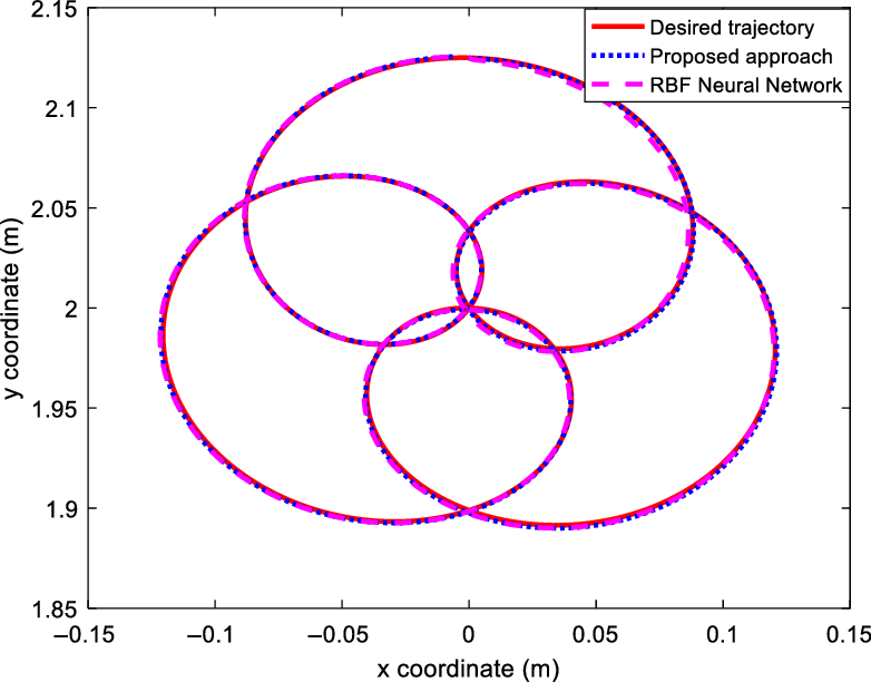
The object path tracking in the XY plane.

Position and orientation tracking errors.

The angles of the first manipulator joints.

The angles of the second manipulator joints.

Control signals of the first manipulator.

Control signals of the second manipulator.

The internal force for the first manipulator.

The internal force for the second manipulator.

The position estimation error.

The estimation performance of
 ${\bf{h}}(t)$
.

Trajectory tracking in the absence of
 ${\hat{\bf h}}(t)$
in (29).

Thus, the vectors
 ${\bf{s}}$
,
 ${\bf{r}}$
and
 ${{\tilde{\bf W}}_{\bf{h}}}$
are uniformly ultimately bounded. Notice that regulating
 ${\bf{r}}(t)$
and
 ${\bf{s}}(t)$
confirms the regulation of
 ${{\bf{e}}_o}(t)$
and
 ${{\tilde{\bf x}}_o}(t)$
, respectively. According to (29) the control signals
 ${\bf{u}}$
,
 ${\bf{v}}$
(from (34)) and so
 ${\bf{h}}(t)$
is bounded that guarantees boundedness of
 ${{\ddot{\bf x}}_o}$
in (21). The following equation, obtained from (20), (29), and (34), shows that internal force errors are bounded.
 \begin{align} ({{\bf{F}}_{Id}} - {{\bf{F}}_I}) & = {({{\bf{I}}_n} + {{\bf{K}}_I})^{ - 1}}\left\{ {{{({\bf{J}}_o^T({{\bf{x}}_o}))}^ + }({{\bf{M}}_c}({{\bf{x}}_o}){{{\ddot{\bf x}}}_o} + {{\bf{C}}_c}({{\bf{x}}_o},{{{\dot{\bf x}}}_o}){{{\dot{\bf x}}}_o} + } \right. \nonumber \\ & \quad \left. {{{\bf{G}}_c}({{\bf{x}}_o}) + {\boldsymbol{\unicode{x1D6AB} }}({{\bf{x}}_o},{\bf{v}}) - {\bf{u}})} \right\}\end{align}
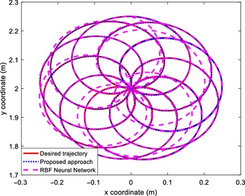
The object trajectory tracking in the XY plane.

Position and orientation tracking errors.

The angles of the first manipulator joints regarding the highly complex trajectory.

The angles of the second manipulator joints regarding the highly complex trajectory.

Control signals of the first manipulator.

Control signals of the second manipulator.

It is clear that the force error is bounded and inversely proportional to the gain matrix
 $({{\bf{I}}_n} + {{\bf{K}}_I})$
. It can be decreased to an arbitrarily small value with a sufficiently large gain.
Remark 3: It should be noted that various users may demand different performance indices from a given system. Whether or not the control accuracy and performance are adequate entirely depends on the user. If more precision is required, the designer can adjust the control factors, including the number of regressor terms or other design parameters, to improve the uncertainty compensation and function estimation. The number of terms in the basis functions is chosen by assigning an arbitrary one first. The number is dropped if the performance is acceptable; otherwise, it is raised. The parameters are assigned based on the following procedure:
-
1. Design
 $\alpha \in \Re $
.
-
2. Choose
${{\boldsymbol{\unicode{x1D6CB} }}_p}$
such that
$\alpha\underline{\boldsymbol{\unicode{x1D6CB}}}_{p}\,>\,1$
. -
3. Choose the nonlinear damping gain satisfying
${k_n} \gt 0.5$
. -
4. Obtain
${{\boldsymbol{\unicode{x1D6CB} }}_c}$
and
${{\boldsymbol{\unicode{x1D6CB} }}_1}$
from (46) and (47). -
5. Obtain
${{\boldsymbol{\unicode{x1D6CB} }}_0}$
from (39).


5. Numerical Evaluation
To apply the designed controller, a cooperative robotic system comprised of two 3-DOF manipulators handling a rigid object is considered as Fig. 2. Detailed information of system modeling (i.e., the manipulators Jacobian, gravity terms, Coriolis and centripetal matrix, and the inertia matrix) is given in ref. [Reference Uchiyama and Dauchez53]. The two manipulators are represented by the indices i = 1,2 throughout the simulation. Suppose that the reference frame is located in the middle of two robots and at the same distance from them. The numerical values of robot parameters are considered as
 ${{\rm l}_{1,1}} = {{\rm l}_{2,1}} = 2.05\,{\rm m}$
,
 ${{\rm l}_{1,2}} = {{\rm l}_{2,2}} = 2.05\,{\rm m}$
, and
 ${{\rm l}_{1,3}} = {{\rm l}_{2,3}} = 0.5\,{\rm m}$
showing each link length.
 ${{\rm m}_{1,1}} = {{\rm m}_{2,1}} = 1\,{\rm kg}$
,
 ${{\rm m}_{1,2}} = {{\rm m}_{2,2}} = 1\,{\rm kg}$
, and
 ${{\rm m}_{1,3}} = {{\rm m}_{2,3}} = 0.3\,{\rm kg}$
denote the link masses.
 ${{\rm I}_{1,1}} = {{\rm I}_{2,1}} = 0.7\,{\rm kg}{{\rm m}^2}$
,
 ${{\rm I}_{1,2}} = {{\rm I}_{2,2}} = 0.5\,{\rm kg}{{\rm m}^2}$
, and
 ${{\rm I}_{1,3}} = {{\rm I}_{2,3}} = 0.3\,{\rm kg}{{\rm m}^2}$
are the links moments of inertia. The exact values of motor model parameters are set to
 ${{\bf{R}}_1} = {{\bf{R}}_2} = diag(2.1,2.1,2.1)[\Omega ]$
,
 ${{\bf{J}}_{a1}} = {{\bf{J}}_{a2}} = diag(2 \times {10^{ - 4}},2 \times {10^{ - 4}},2 \times {10^{ - 4}})[kg.{m^2}]$
,
 ${{\bf{r}}_1} = {{\bf{r}}_2} = diag({10^{ - 2}},{10^{ - 2}},{10^{ - 2}})$
,
 ${{\bf{k}}_{a1}} = {{\bf{k}}_{a2}} = {{\bf{k}}_{b1}} = {{\bf{k}}_{b2}} = diag(0.189,0.219,0.202)[N.m/A]$
and
 ${{\bf{b}}_{a1}} = {{\bf{b}}_{a2}} = diag(1.48,0.817,1.38) \times {10^{ - 3}}[N.m.s/rad]$
. The object was dynamically modeled as (8)-(10) where
 \begin{align} {{\bf{D}}_o}({{\bf{x}}_o}) = \left[ {\begin{array}{*{20}{c@{\quad}c@{\quad}c}}{{m_o}} & 0 &0\\0& {{m_o}} &0\\0& 0 &{{I_o}}\end{array}} \right],{\rm{ }}{{\bf{G}}_o}({{\bf{x}}_o}) = \left[ {\begin{array}{*{20}{c}}0\\{{m_o}g}\\0\end{array}} \right]\end{align}
where the inertia of the object is represented by
 ${I_o}$
, and its mass is
 ${m_o}$
. The grasp matrix is given in the form of (9), where
 \begin{align} {{\bf{J}}_{o1}}({{\bf{x}}_o}) = \left[ {\begin{array}{*{20}{c@{\quad}c@{\quad}c}}1 &0& {{l_{1l}}\sin ({x_{o3}})}\\0& 1& { - {l_{1l}}\cos ({x_{o3}})}\\0 &0 &1\end{array}} \right],\quad {\rm{ }}{{\bf{J}}_{o2}}({{\bf{x}}_o}) = \left[ {\begin{array}{*{20}{c@{\quad}c@{\quad}c}}1& 0& { - {l_{2l}}\sin ({x_{o3}})}\\0 &1 &{{l_{2l}}\cos ({x_{o3}})}\\0 &0& 1\end{array}} \right]\end{align}
The internal force for the first manipulator.

The internal force for the second manipulator.

The position estimation error.

The approximation performance of
 ${\bf{h}}(t)$
.

Trajectory tracking in the absence of
 ${\hat{\bf h}}(t)$
in (29).

In this equation, the distance from the object COM and the ith end-effector is denoted by
 ${l_{il}}$
, which is twice the object length.
 ${m_o}$
and
 ${I_o}$
are set to 0.2 kg and 0.1 kgm2, respectively. It is assumed that no information from the dynamics
 ${{\bf{M}}_c}({{\bf{x}}_o})$
,
 ${{\bf{C}}_c}({{\bf{x}}_o},{{\dot{\bf x}}_o})$
, and
 ${{\bf{G}}_c}({{\bf{x}}_o})$
is available. We suppose that an external disturbance is given by
 \begin{align} {{\boldsymbol{\unicode{x1D6BB} }}_{d,i}}(t) = \left[ {\begin{array}{*{20}{c}}{0.4\cos (2t)}\\{0.1\sin (t) + \cos (2t)}\\{0.2\sin (t)}\end{array}} \right]\!,\quad {\rm{ i = 1,2}}\end{align}
which is added to each robot manipulator from the input channel. The values of the proposed scheme parameters are considered as
 $\alpha = 1$
,
 ${{\boldsymbol{\unicode{x1D6CB} }}_p} = diag{(10)_{3 \times 3}}$
,
 ${{\boldsymbol{\unicode{x1D6CB} }}_c} = diag{(3)_{3 \times 3}}$
,
 ${{\boldsymbol{\unicode{x1D6CB} }}_1} = diag{(113)_{3 \times 3}}$
,
 ${{\boldsymbol{\unicode{x1D6CB} }}_0} = diag{(111)_{3 \times 3}}$
,
 ${k_n} = 1$
, and
 ${{\bf{K}}_I} = diag{(100)_{6 \times 6}}$
. To estimate the lumped uncertainty
 ${\bf{h}}(t)$
, the first three terms of the BTO are selected. So,
 ${{\hat{\bf W}}_{\bf{h}}} \in {\Re ^{9 \times 3}}$
. The initial values of the adaptive parameters are set equal to zero. The convergence rate matrix is selected as
 ${{\bf{Q}}_{\bf{h}}} = {10^{ - 4}} \times {{\bf{I}}_9}$
, where
 ${{\bf{I}}_9}$
denotes the 9×9 identity matrix. At this point, assume that the estimation error is acceptable and therefore negligible, that is,
 ${\sigma _{\bf{h}}} = 0$
.
The suggested BTO-based estimator’s performance is compared to another existing approximator to evaluate its efficiency. To this mean, the RBF neural network is integrated into the proposed control method, as the estimator, to approximate uncertainties and external disturbances. The RBFNN output is derived from a linear combination of the neural network’s hidden layer outputs. Consider that the inputs of the RBFNN are the elements of the vector
 $\varpi (t) = {\left[ {\begin{array}{*{20}{c}}{{\hat{\bf x}}_o^T(t)}\quad{{\dot{\hat{\bf x}}}_o^T(t)}\end{array}} \right]^T}$
. As a result,
 \begin{align} {{\bf{Z}}_h} = {\left[ {\begin{array}{*{20}{c}}{{\xi _1}}\quad{{\xi _2}}\quad{ \ldots }\quad{{\xi _{{N_1}}}}\end{array}} \right]^T} \in {\Re ^{{N_1}}}\end{align}
with
 \begin{align} {\xi _i} = \exp \left( - \frac{{{{\left\| {\varpi (t) - {c_i}} \right\|}^2}}}{{\delta _i^2}}\right)\,\,\,\,\,\,i = 1,2, \ldots ,{N_1}\end{align}
where
 ${N_1}$
stands for the hidden layer neurons number. The RBFNN weights are initially set equal to zero. The values of the observer/controller parameters are considered the same as previously stated values. The values of
 ${c_i}$
and
 ${\delta _i}$
are considered as
 \begin{align} \begin{array}{l}{c_1} = {\left[ {\begin{array}{*{20}{c}}{\begin{array}{*{20}{c}}{\begin{array}{*{20}{c}}{ - 2 \times {{10}^{ - 2}}}\;\;\;\;\;{ - 2 \times {{10}^{ - 2}}}\;\;\;\;\;{ - 2 \times {{10}^{ - 2}}}\;\;\;\;\;{ - 4.5}\;\;\;\;\;{ - 4.5}\;\;\;\;\;{ - 4.5}\end{array}}\end{array}}\end{array}} \right]^T}\\[4pt] {c_2} = {\left[ {\begin{array}{*{20}{c}}{\begin{array}{*{20}{c}}{\begin{array}{*{20}{c}}{ - 1.6 \times {{10}^{ - 3}}}\;\;\;\;\;{ - 1.6 \times {{10}^{ - 3}}}\;\;\;\;\;{ - 1.6 \times {{10}^{ - 3}}}\;\;\;\;\;{ - 3.6}\;\;\;\;\;{ - 3.6}\;\;\;\;\;{ - 3.6}\end{array}}\end{array}}\end{array}} \right]^T}\\[4pt] {c_3} = {\left[ {\begin{array}{*{20}{c}}{\begin{array}{*{20}{c}}{\begin{array}{*{20}{c}}{ - 1.2 \times {{10}^{ - 3}}}\;\;\;\;\;{ - 1.2 \times {{10}^{ - 3}}}\;\;\;\;\;{ - 1.2 \times {{10}^{ - 3}}}\;\;\;\;\;{ - 2.7}\;\;\;\;\;{ - 2.7}\;\;\;\;\;{ - 2.7}\end{array}}\end{array}}\end{array}} \right]^T}\\[4pt] {c_4} = {\left[ {\begin{array}{*{20}{c}}{\begin{array}{*{20}{c}}{\begin{array}{*{20}{c}}{ - 8 \times {{10}^{ - 3}}}\;\;\;\;\;{ - 8 \times {{10}^{ - 3}}}\;\;\;\;\;{ - 8 \times {{10}^{ - 3}}}\;\;\;\;\;{ - 1.8}\;\;\;\;\;{ - 1.8}\;\;\;\;\;{ - 1.8}\end{array}}\end{array}}\end{array}} \right]^T}\\[4pt] {c_5} = {\left[ {\begin{array}{*{20}{c}}{\begin{array}{*{20}{c}}{\begin{array}{*{20}{c}}{ - 4 \times {{10}^{ - 3}}}\;\;\;\;\;{ - 4 \times {{10}^{ - 3}}}\;\;\;\;\;{ - 4 \times {{10}^{ - 3}}}\;\;\;\;\;{ - 0.9}\;\;\;\;\;{ - 0.9}\;\;\;\;\;{ - 0.9}\end{array}}\end{array}}\end{array}} \right]^T}\\[4pt] {c_6} = {\left[ {\begin{array}{*{20}{c}}{\begin{array}{*{20}{c}}{\begin{array}{*{20}{c}}0\;\;\;\;\;0\;\;\;\;\;0\;\;\;\;\;0\;\;\;\;\;0\;\;\;\;\;0\end{array}}\end{array}}\end{array}} \right]^T}\end{array}\end{align}
 \begin{align} {\delta _1} = 4,\,\,{\delta _2} = 3,\,\,{\delta _3} = 2,\,\,{\delta _4} = 2,\,\,{\delta _5} = 1,\,\,{\delta _6} = 0.5\end{align}
These values are achieved through trial and error and are not optimized.
5.1 Results: Performance evaluation and comparison
To evaluate the controller functioning, two different paths are considered.
Case 1: Simple path
The desired object trajectory is chosen as
 \begin{align} {{\bf{x}}_{od}}(t) = {\left[ {\frac{{\sin (2t) + \sin (8t)}}{{16}},2 + \frac{{\sin (2t + 1.6) + \sin (8t + 1.6)}}{{16}},0} \right]^T}\end{align}
The desired internal force level is
 ${{\bf{F}}_{Id}}(t) = {[\begin{array}{*{20}{c}}0\;\;\;0\;\;\;0\;\;\;0\;\;\;0\;\;\;0\end{array}]^T}$
. The two 3-DOF arms are initiated at rest, and the joint positions are
 ${\bf{q}} = {\left[ {\begin{array}{*{20}{c}}{2.5968}\;\;\;{ - 2.0519}\;\;\;{ - 0.5448}\;\;\;{0.5448}\;\;\;{2.0519}\;\;\;{0.5448}\end{array}} \right]^T}$
. It is presumed that the initial values of the actual and desired angles are the same. The suggested controller-observer and the RBFNN approximator-based controller are used to control the robot using the stated settings. In Fig. 3, the actual and desired coordinates of the object’s center are shown. Despite the existence of uncertainties and disturbances, the arm successfully tracks the desired path, as shown in the figure. Figure 4 presents tacking errors to the x and y coordinates and orientation, which are tiny and UUB. The joint angles for the first and second arms are presented in Figs. 5 and 6, respectively. Both controllers are capable of fulfilling a good tracking performance. The control signals applied on the manipulators are shown in Figs. 7 and 8. The results present the boundedness and smoothness of the control signals. Figures 9 and 10 show the results of the internal force tracking. According to these figures, the internal forces are efficiently controlled. Figure 11 shows the position approximation errors. This figure presents the boundedness of the estimation error. The estimated lumped uncertainties are presented in Fig. 12. Based on this figure, both methods can estimate the uncertainty exactly. The outcomes are also simulated without the term
 ${\hat{\bf h}}(t)$
in (29) to demonstrate its importance. Since the approximation error
 ${{\boldsymbol{\unicode{x1D6C6} }}_{\bf{h}}}$
is not neglected, this is the best scenario for examining the system uniformly ultimately bounded stability. In other words, the approximation error,
 ${{\boldsymbol{\unicode{x1D6C6} }}_{\bf{h}}}$
, has the maximum value in this scenario. The relative path tracking result is shown in Fig. 13.
Due to the universal approximation feature of these approaches, the suggested BTO-based and RBFNN estimators perform nearly the same. Nevertheless, the RBFNN’s regressor vector has more tunable factors (such as the center and width of the Gaussian units), and selecting the appropriate values for these factors is time-consuming owing to trial and error. Besides, unlike fuzzy/neural network techniques that rely on system states as inputs to approximate functions and generate a regressor vector, the suggested FAT-based methodology does not rely on system states. That is because these estimators treat uncertainties as time-varying functions rather than functions of multiple system states. Furthermore, the FAT-based adaptive controller is not affected by the number of system states, which is the most essential factor in determining the dimension of the basis function vectors. As a result, compared to RBFNN, the FAT-based controller has a lower computational load and a simpler structure.
Case 2: Highly complex path tracking
The second desired path is constructed as follows to demonstrate the efficacy of the introduced controller in applications requiring accurate tracking of fast and extremely complicated paths.
 \begin{align} {{\bf{x}}_{od}}(t) = \left[ {\begin{array}{*{20}{c}}{0.125sin(2t) + 0.125sin(11t)}\\{2 + 0.125sin\left( {2t + 1.6} \right) + 0.125sin\left( {11t + 1.6} \right){\rm{ }}}\\0\end{array}} \right]\end{align}
where the initial robot configuration is as
 ${\bf{q}} = \left[{2.5607}\;\;\;{ - 1.9798}\;\;\;{ - 0.5809}\;\;\; {0.5809}\;\;\;{1.9798}\;\;\;{0.5809} \right]^{T}$
. This trajectory is critical because it requires quick and intricate interactions between the cooperative robot manipulators’ dynamics. The initial and desired joint positions are assumed to be the same. All simulation configurations are identical to those utilized in case 1. Figures 14 through 24 show the results of this simulation. Figure 14 illustrates the object tracking performance in the XY plane. As the results reveal, the BTO-based uncertainty approximation outperforms the RBF neural network-based uncertainty approximation significantly. Figure 15 depicts the y- and x-coordinate position errors and the orientation error. By selecting appropriate control parameters, these errors can be reduced. The joint angles for the first and second manipulators are presented in Figs. 16 and 17, respectively. Figures 18 and 19 illustrate the bounded and smooth control signals. Figures 20 and 21 show the internal force tracking performance. Figure 22 presents the position estimation errors. The estimated lumped uncertainties are revealed in Fig. 23. This figure demonstrates the precise uncertainty approximation capability of the proposed BTO-based approach. The test is again carried out without term
 ${\hat{\bf h}}(t)$
in (29) to present its importance. The path tracking result under this condition is illustrated in Fig. 24. Based on this figure, the developed approximator has an essential role in fulfilling an efficient tracking performance.
6. Conclusion
This work deals with the force-position tracking problem of an object handled by multiple cooperative arms with unknown external disturbances and uncertainties. It is considered that joint speeds are unavailable, and only joint positions can be measured. Regarding the fact, first, the dynamic model of the system, including the robotic arms and the handled object, is obtained. Then, an observer-based control scheme is developed using the Bernstein-type operators. The Lyapunov direct method is utilized to examine the system’s stability thoroughly. The outcomes show that system errors are bounded. Since the suggested method is regressor-free, it avoids the drawbacks of adaptive approaches. One of the benefits of the suggested method is that it is model-free, making it robust in the face of unmodeled dynamics. It is important to note that knowing the uncertainty bounds is not required in this approach. In addition, unlike many typical controllers, this study considers the voltage signal rather than the torque as the control signal, and the motor dynamics are not ignored. Two 3-DOF cooperative robotic arms are used to analyze the performance of the adaptive BTO-based controller. The results demonstrate that the proposed scheme is robust in the existence of disturbances and unmodulated dynamics. Future research could expand the presented approach to a fractional-order structure, which would allow it to deal with more severe uncertainties and perturbations. Future studies could also concentrate on applying the notion to teleoperation systems, such as surgical robots that collaborate. Moreover, the estimator can be applied to under-actuated cooperating systems.
7. Compliance with Ethical Standards
Authors declare that the manuscript has not been submitted to more than one journal for simultaneous consideration and it has not been published previously (partly or in full). In addition, this study has not been split up into several parts to increase the quantity of submissions. No data have been fabricated or manipulated to support the conclusions. Moreover, no data, text, or theories by others are presented as if they were our own. Proper acknowledgements to other works have been given.
Funding
No organization has funded this study.
Conflict of interest
The authors declare that they have no conflict of interest.
Research involving Human Participants and/or Animals
Authors declare that there has been no human participant or animal in this research.
Authors declare that there is no need for informed consent for this paper, since the results have been obtained using computer simulations.