Implications
Missing genotypes on large proportions of livestock animals is a major problem when implementing gene-assisted breeding value estimation for genes with known effect. In this study, we compared different methods. Using mixed model methodology to predict missing genotypes was considered as the practically best method. Gene-assisted breeding value estimation leads to 0% to 22% increase in accuracy for genotyped animals and 0% to 5% increase in accuracy for ungenotyped animals. Especially for traits with low heritability, also ungenotyped animals benefit from gene-assisted breeding value estimation. Results may indicate that also genomic selection would be beneficial for ungenotyped animals, especially at low heritability.
Introduction
In the last 20 years, many studies have been carried out to find quantitative trait loci (QTL) for quantitative traits in livestock. In some cases, the causative mutation was identified, e.g. DGAT1 in dairy cattle for milk yield and milk composition (Grisart et al., Reference Grisart, Coppieters, Farnir, Karim, Ford, Berzi, Cambisamo, Mni, Simon, Spelman, Georges and Snell2002; Winter et al., Reference Winter, Kramer, Werner, Kollers, Kata, Durstewitz, Buitkamp, Womack, Thaller and Fries2002) and IGF2 in pigs for body weight (Van Laere et al., Reference Van Laere, Nguyen, Braunschweig, Nezer, Collete, Moreau, Archibald, Haley, Buys, Tally, Andersson, Georges and Andersson2003). Marker-assisted and gene-assisted selection have been shown to increase genetic gain in breeding programs with a higher increase for traits with low heritability (Lande and Thompson, Reference Lande and Thompson1990; Meuwissen and Goddard, Reference Meuwissen and Goddard1996; see reviews in Weller, Reference Weller2001; Dekkers and Van der Werf, Reference Dekkers and Van der Werf2007; Weller, Reference Weller2007). Gene-assisted selection increases genetic gain more than marker-assisted selection, because no recombination takes place between the marker and QTL, and therefore estimated breeding values (EBV) are predicted with higher accuracy with gene-assisted breeding value estimation (Villanueva et al., Reference Villanueva, Pong-Wong and Woolliams2002). Finding all genes is, however, more difficult and more resource-demanding (Dekkers, Reference Dekkers2004). To circumvent this, Meuwissen et al. (Reference Meuwissen, Hayes and Goddard2001) proposed genomic selection, where breeding values are predicted based on genome-wide estimated marker effects using dense single nucleotide polymorphism (SNP) maps, utilizing that SNP are in linkage disequilibrium with genes of interest.
Different procedures have been proposed for gene- and marker-assisted breeding value estimation, some being also used for QTL detection. The methods can be classified into two groups: (i) model QTL effects as random effects and use an inverse identity-by-descent matrix (IBD) to account for relationships between haplotypes of related animals (Fernando and Grossman, Reference Fernando and Grossman1989) and (ii) model gene and/or markers as fixed or random effects (Weller, Reference Weller2001; Dekkers and Van der Werf, Reference Dekkers and Van der Werf2007) or regression on gene content (number of copies of B-allele in the case of B and b-alleles) in the case of bi-allelic genes (e.g. Gengler et al., Reference Gengler, Mayeres and Szydlowski2007 and Reference Gengler, Abras, Verkenne, Vanderick, Szydlowski and Renaville2008). No studies have compared both methods for gene-assisted breeding value estimation. It is expected that directly modeling gene effects or regression on gene contents would yield higher accuracies of EBV than modeling haplotype effects with an IBD method, because fewer effects need to be estimated. The advantage of using the IBD method is that it is more generic and can be used when either the gene is known or unknown.
Until now, gene-assisted, marker-assisted and genomic breeding value estimation has been implemented on a limited scale. One of the main challenges is to include both genotyped and ungenotyped animals in breeding value estimation. Including genotyped and ungenotyped animals in one evaluation is not only for practical ease, but is important also to optimize the usage of information. Several methods have been proposed to deal with missing genotypes. Hoeschele (Reference Hoeschele1993) and Meuwissen and Goddard (Reference Meuwissen and Goddard1999) proposed methods to eliminate equations of QTL effects of ungenotyped animals by absorption, which requires an adapted variance–covariance matrix among breeding values and QTL effects. When the gene is known, iterative peeling methods can be used to predict genotype probabilities (Van Arendonk et al., Reference Van Arendonk, Smith and Kennedy1989; Fernando et al., Reference Fernando, Stricker and Elston1993; Thallman et al., Reference Thallman, Bennett, Keele and Kappes2001a and Reference Thallman, Bennett, Keele and Kappes2001b; Meuwissen, Reference Meuwissen2006). In the case of bi-allelic genes, the gene content can be predicted using mixed model methodology (MM), where (un)known genotypes are treated as (missing) phenotypes using the additive genetic relationship matrix to predict missing genotypes (Gengler et al., Reference Gengler, Mayeres and Szydlowski2007 and Reference Gengler, Abras, Verkenne, Vanderick, Szydlowski and Renaville2008). Gengler et al. (Reference Gengler, Mayeres and Szydlowski2007) compared single-marker iterative peeling with the MM method and concluded that MM performed well and is attractive for implementation of gene-assisted breeding value estimation in large populations. When using the IBD method, Totir et al. (Reference Totir, Fernando, Dekkers, Fernandez and Guldbrandtsen2004) presented approximations to calculate IBD matrices when some animals are not genotyped. Meuwissen (Reference Meuwissen2006) proposed to calculate inverse IBD matrices based on the genotype probabilities that are calculated by multiple-marker iterative peeling. The method of Meuwissen (Reference Meuwissen2006) is deterministic in nature making it possible to calculate inverse IBD matrices based on linkage analysis information (IBD–LA) for large populations. Until now, no studies have compared regression on gene content with IBD–LA method when dealing with missing genotypes in gene-assisted breeding value estimation and the difference in accuracy of total breeding value is unknown.
The overall objective was to compare different methods to deal with missing marker genotypes on accuracy of gene-assisted breeding value estimation for identified bi-allelic genes using Monte Carlo simulation. The detailed objectives of this article were: (i) to compare accuracy of gene-assisted breeding value estimation with missing marker genotypes when regressing on predicted gene content or using IBD–LA, (ii) to extend the single-marker MM (S-MM) method to multiple-marker MM (M-MM) and (iii) to compare multiple-marker iterative peeling (MIP), single-marker iterative peeling (SIP), M-MM and S-MM on accuracy of gene-assisted breeding value estimation using regression on gene content. Two scenarios of missing marker genotypes were evaluated for different values of the heritability and proportion of genetic variance explained by the QTL. In addition, situations with sex-linked traits and juvenile animals without phenotypes were considered.
Material and methods
Scenarios and outline of simulation
Outline
In practice, usually a limited number of animals is genotyped. Mainly (potential) sires and some potential female selection candidates are genotyped. The vast majority of the animals that are phenotypically recorded do not have marker genotypes. However, in gene-assisted breeding value estimation, the aim is that phenotypic information of ungenotyped animals is also used for estimation of QTL effects. Therefore, we simulated three genotyping scenarios: (i) only sires and males in the last generation are genotyped and (ii) all males are genotyped and (iii) all animals are genotyped. If animals are genotyped, then they are genotyped for the QTL and 10 flanking markers. One trait was simulated with one bi-allelic QTL, a polygenic and a residual effect. The simulation scheme represented a nested full-sib half-sib design (multiple offspring per mating and dam nested within sire) with discrete generations, which is common in commercial breeding programs. One trait was simulated, which was recorded on all animals once. Because some of the methods applied rely on linkage disequilibrium (LD) between markers and QTL, first 100 generations of random mating were performed prior to the data collection scheme (generations 101 to 105), which will be called the LD generations.
LD generations
Each generation of 50 sires and 50 dams were randomly mated. The QTL and 20 bi-allelic markers were placed on one chromosome of 1 M length. The QTL was placed in the middle of the chromosome and the markers were equally spaced at 5 cM (first marker was at 2.5 cM and the last at 97.5 cM). The QTL was in the middle of the marker bracket between marker 10 and 11, resulting in that both direct flanking markers are at a distance of 2.5 cM. In the founder generation, all markers and the QTL were in linkage equilibrium and had an allele frequency of 0.5. The QTL variance  varied between 5% and 25% of the total genetic variance, when the allele frequency is 0.5. The allele substitution effect was set to:
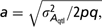
assuming that the allele frequencies p and q are 0.5, which is the case in the base generation. Recombination rates were calculated using Haldane mapping function (Haldane, Reference Haldane1919). During the LD generations, some markers or the QTL became fixed due to drift.
Data collection scheme
After establishing LD, each generation of 50 sires and 250 dams were selected based on conventional BLUP–EBV and randomly mated to produce 2000 offspring (1000 males and 1000 females). Each sire was mated to five dams and each dam produced eight offspring resulting in that each sire had 40 half-sib offspring, five full-sib groups of eight full-sibs. In total, five generations of phenotypic data (generations 101 to 105) were created and used in breeding value estimation (10 000 animals in total). The animals of generation 101 served as base generation in the pedigree. The generations 102 to 104 were used to create gametic phase disequilibrium (Bulmer, Reference Bulmer1971). On each side of the QTL, five markers were selected with an allele frequency between 0.05 and 0.95 in generation 105 and that were as close as possible to the QTL. Results were based on 100 effective replicates after discarding the replicates with minor allele frequency of the QTL in the last generation (generation 105) less than 0.05 or with less than five polymorphic markers on either side of the QTL. Due to fixation of some markers, the average marker distance over all replicates was 0.058.
In generation 101, polygenic effects were sampled from  , where
 is the polygenic genetic variance. In subsequent generations polygenic effects were sampled from
 , where f p is the average inbreeding coefficient of the parents. Inbreeding coefficients were calculated using the Meuwissen and Luo (Reference Meuwissen and Luo1992) algorithm. Residual effects were sampled as
 , where
 is the residual variance. The total phenotype was
 , where A qtl is −a, 0 and a for, respectively, the QTL genotypes 11, 12 and 22.
Parameter values in simulation
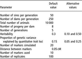
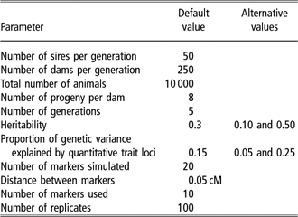
The overall heritability was 0.1, 0.3 and 0.5 and the QTL explained 5%, 15% and 25% of the total genetic variance when the allele frequency was 0.5 as it was in the founder generation. The phenotypic variance was 1.0 in all situations when the allele frequency of the QTL was 0.5. The realized variance of the QTL was lower due to deviations of the allele frequency from 0.5. Averaged over all replicates, the average allele frequency of the negative QTL allele was 0.63 in generation 101 before selection started and deviated from 0.5, because in replicates with allele frequencies closer to 0, the QTL was more likely to get fixated due to selection. The used parameter values are listed in Table 1. In addition to the situation where all animals had phenotypic records, two other scenarios were evaluated using the default parameters: (i) juveniles without phenotypic records and (ii) a trait that is measured only on females, e.g. female reproduction traits.
Parameter values for simulation
Breeding value estimation
Conventional BLUP
A conventional genetic evaluation was performed using an animal model:

where u con is the estimated breeding value with variance  (
 was re-estimated in generation 101;
 ). The overall mean, μ, was fixed and u con was random and the inverse additive genetic relationship matrix (A−1) was used to account for covariances between related animals. In all cases, MM equations were solved using MiX99, which makes use of the preconditioned conjugate gradient algorithm (Lidauer and Stranden, Reference Lidauer and Stranden1999). The MM equations were considered converged when the relative difference between left-hand and right-hand side of the MM equations was smaller than 1.0 × 10⁻¹⁰.
Gene-assisted (GA)-BLUP with regression on predicted gene content
In this case, equation (1) was extended with a random regression on the predicted gene content, either from MIP/SIP or M-MM/S-MM (see later):

where u pol is the estimated polygenic breeding value with variance  , b is the random regression coefficient for the QTL effect with
 and
 is the predicted gene content (see Prediction of gene content section). Regression on gene content was modeled as a random effect to have the QTL effect, in both this method and the IBD method, as a random effect. In this case, the difference between modeling gene content as a random or as a fixed effect would be minor. Results were very robust against small errors in the used variance component. In addition, when many SNP would be included in the model such as in genomic selection, it is advantageous to include them as random effects rather than as fixed effects (Meuwissen et al., Reference Meuwissen, Hayes and Goddard2001).
GA-BLUP with IBD method
In this case, equation (1) was extended with paternal (h pat) and maternal haplotype effects (h mat):

The relationship between the haplotypes was accounted for by using an inverse IBD matrix (G−1) in the MM equations (Fernando and Grossman, Reference Fernando and Grossman1989). The MM equations in matrix notation are:

where X, Z and W are the design matrices for fixed effects, polygenic breeding values and haplotype effects, respectively, and α and β are respectively the variance ratios for the polygenic breeding values and haplotype effects. The variance of the haplotype effects was half the variance at the QTL ( ), because the QTL effect per animal is explained by two haplotypes. The
 was re-estimated in the base generation (generation 101, first generation after LD generations) to account for changes in allele frequency of the QTL during the LD generations (
 ). For all methods, true simulated variances in generation 101 were used to avoid using restricted maximum likelihood to estimate variance components, which would have added substantial computing time and was outside the scope of this study.
Prediction of gene content
MIP (multiple-marker iterative peeling)
Multiple-marker iterative peeling (Meuwissen, Reference Meuwissen2006) was used to calculate genotype probabilities at the QTL locus making use of 10 flanking markers (MIP). The algorithm is suitable for large pedigrees. Briefly, the method is applied to one marker at a time, where the transmission probabilities (probability of offspring inheriting genotype X when the parents have genotypes Y and Z) account for the inheritance at surrounding loci. In addition to the algorithm explained in Meuwissen (Reference Meuwissen2006), the current algorithm uses LD information to infer genotype probabilities as explained in Appendix 1. Furthermore, the same algorithm was used without flanking markers (SIP). The comparison between MIP and SIP gives insight in the advantage of using flanking markers (i.e. LA information). The expected gene content was calculated as  where gpi is the genotype probability and gci is the gene content of genotype i, i.e. 2, 1, 0 for respectively 22, 12 and 11.
S-MM (single-marker mixed model)
The single-marker mixed model method (Gengler et al., Reference Gengler, Mayeres and Szydlowski2007 and Reference Gengler, Abras, Verkenne, Vanderick, Szydlowski and Renaville2008) was used to predict gene content. The model for S-MM was:

where μgc is the overall mean (twice the allele frequency of allele 2 in the base generation), d is the EBV for gene content and egc is the residual of gene content. The MM equations are:
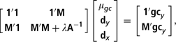
where 1 and M are the design matrices for fixed effects (only μ) and EBV for gene content (d), A−1 is the inverse additive genetic relationship matrix, λ is the variance ratio of residual variance and additive genetic variance for gene content allowing for a small proportion of genotyping errors  , d is a vector with the EBV for gene content with dy for genotyped animals and dx for ungenotyped animals (expected gene content:
 ) and gcy is the vector with observed gene contents. Gene contents of animals not genotyped were set to missing. The S-MM method does not account for information of flanking markers.
M-MM (multiple-marker mixed model)
In this article, we propose a simple multivariate extension using other marker gene contents as correlated information, which requires the correlation between markers. The correlation r was calculated on all marker genotypes, assuming that all animals are genotyped. The squared correlation r 2 is a measure of LD (Hill and Robertson, Reference Hill and Robertson1968). The average r 2 between adjacent markers was 0.048. The MM equations are:
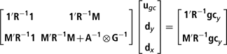
where the residual variance–covariance matrix  (
 ) and the genetic variance–covariance matrix for n markers
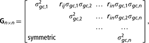
where n is 11 (10 markers + QTL) in our study and  . When values of rij were larger than 0.98 (smaller than −0.98), the value of rij was set to 0.98 (−0.98) to avoid singularities in the matrix. MiX99 was used to solve the MM equations for S-MM and M-MM (Lidauer and Stranden, Reference Lidauer and Stranden1999). The MM equations were considered converged when the relative difference between left-hand and right-hand side of the MM equations was smaller than 1.0 × 10⁻¹⁰.
Prediction of IBD probabilities
Multiple iterative peeling was used to calculate segregation indicator probabilities based on predicted genotype probabilities. Segregation indicator probabilities were adjusted when the locus itself was uninformative (e.g. homozygous parent, both parents are heterozygous) using information of the nearest informative loci on both sides of the QTL (Meuwissen, Reference Meuwissen2006). These segregation indicator probabilities were used to calculate inverse IBD matrices at the marker locus using Fernando and Grossman (Reference Fernando and Grossman1989) rules in a recursive manner. When the paternal segregation indicator probabilities were larger than 0.95 (smaller than 0.05), offspring received the paternal (maternal) haplotype. The inverse IBD matrices were sparsely stored to save memory. The base haplotypes were assumed unrelated. Therefore, the inverse IBD matrices contained only linkage analysis information (IBD–LA).
Evaluation of accuracy of GA-BLUP
The accuracy of GA-BLUP was assessed by the accuracy of the estimated QTL–EBV, polygenic EBV and total EBV. The estimated QTL–EBV was calculated as  for model (2) and as
 for model (3). The total EBV was calculated as the sum of the QTL–EBV and the polygenic EBV. The accuracy was calculated as the correlation between the true and estimated breeding values. Results were averaged over the 100 replicates.
Results
Comparison of regression on predicted gene content with IBD–LA
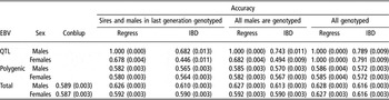
Table 2 shows the accuracies of EBV for regression on gene content and the IBD–LA method when applying GA-BLUP. In the scenarios with missing genotypes, MIP was used to predict gene content for GA-BLUP with regression on gene content. The accuracies were always lower with IBD–LA than with regression on gene content. Note that the accuracy of QTL–EBV with regression on gene content was unity for genotyped animals. Although the allele substitution effects were sometimes under- or overestimated, the signs were always correctly estimated. Since the QTL had two alleles, the correlation between QTL–EBV and the true QTL effect was always one. Genotyped males benefited more from GA-BLUP than ungenotyped females. For ungenotyped females, the benefit of GA-BLUP was negligible. Accuracies were slightly higher when all males were genotyped than when only sires and the males in the last generation were genotyped, especially with the IBD–LA method, but the results are similar. The IBD–LA method is more sensitive to the number of genotyped animals than the regression on gene content method.
Accuracies of quantitative trait loci (QTL)–estimated breeding values (EBV), polygenic EBV and total EBV for males and females in the last generation using conventional BLUP (Conblup), regression (Regress) on predicted gene content with multi-marker iterative peeling or using linkage analysis of identity-by-descent relationships method in gene-assisted BLUP when the heritability is 0.30 and the QTL explains 15% of the genetic variance, when only sires and males in last generation are genotyped, when all males are genotyped or when all animals are genotyped

IBD = identity-by-descent relationship method; QTL = quantitative trait loci.
Average of 100 replicates; standard errors within brackets.
Effect of heritability and proportion of genetic variance explained by the QTL
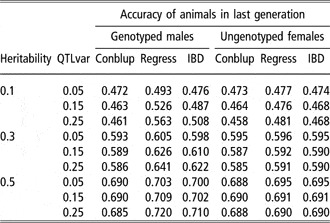
Table 3 shows the accuracies of total EBV with GA-BLUP relative to conventional BLUP. The accuracies increased more with regression on gene content than with IBD–LA. Differences between both methods were largest at low heritability and high QTL variance for genotyped animals, whereas differences were smaller for ungenotyped animals. In most cases, the increase in accuracy was marginal for ungenotyped animals, but the increase was still substantial when the heritability was low and the QTL variance was high.
Accuracy of total estimated breeding value for different combinations of heritability and quantitative trait loci variance (QTLvar) as proportion of the total genetic variance for males and females in the last generation using conventional BLUP (Conblup) or gene-assisted BLUP using either regression on gene content (Regress) or the linkage analysis of identity-by-descent relationships method, when sires and males in the last generation were genotyped

IBD = identity-by-descent relationship method.
Average of 100 replicates; standard errors are 0.004–0.006, 0.003–0.004 and 0.002–0.003 for heritabilities 0.1, 0.3 and 0.5, respectively.
Effect of minor allele frequency
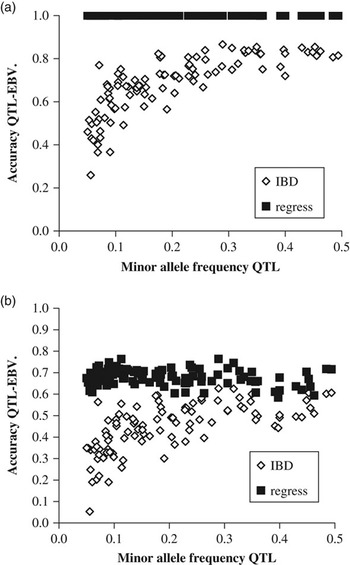
Figure 1 shows the accuracy of QTL–EBV as a function of the minor allele frequency (MAF) of the QTL in the last generation using regression on gene content or IBD–LA for males (panel A) and females (panel B) in the last generation. For both males and females, the accuracy of the QTL–EBV was insensitive to MAF with regression on gene content, whereas it was sensitive to MAF with IBD–LA. With IBD–LA, the accuracy decreased when MAF was lower than 0.2. When MAF was higher than 0.2, no clear trend was observed. Substantial variation was observed between replicates for IBD–LA. For ungenotyped females, both methods showed variation between replicates, especially with IBD–LA. It can be concluded that the accuracy of the GA-BLUP with IBD–LA decreases, when the minor allele frequency of the QTL is lower than 0.2, whereas the accuracy does not change with regression on gene content.
Accuracy of quantitative trait loci (QTL)–estimated breeding value (EBV) as a function of the minor allele frequency of the QTL in the last generation using regression on predicted gene content with multiple-marker iterative peeling or identity-by-descent relationships using linkage analysis (IBD–LA) for genotyped males (panel a) and ungenotyped females (panel b) in the last generation (only sires and males in the last generation are genotyped) when the heritability is 0.30 and the QTL explains 15% of the genetic variance (each point represents one replicate of in total 100 replicates).

Juveniles and female traits
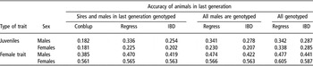
Table 4 shows the accuracies of total EBV for regression on gene content and the IBD approach for juveniles that do not have phenotypes yet and female traits measured only in females (e.g. milk production). For juveniles, accuracies were substantially lower than for animals with a phenotypic record. The increase in accuracy with GA-BLUP in comparison to conventional BLUP was substantial, also for ungenotyped females. The difference between regression on gene content and IBD–LA was larger than when all animals had phenotypes.
Accuracies of total estimated breeding values for traits for males and females in the last generation using conventional BLUP (Conblup), regression (Regress) on predicted gene content with multi-marker iterative peeling or using linkage analysis of identity-by-descent relationships method in gene-assisted BLUP when the heritability is 0.30 and the quantitative trait loci explains 15% of the genetic variance for animals at early age before phenotypes are recorded (juveniles) and traits recorded only in females (female trait) when only sires and males in last generation are genotyped, when all males are genotyped or when all animals are genotyped

IBD = identity-by-descent relationship method.
Average of 100 replicates; standard errors are 0.006–0.007 for juveniles for both sexes, 0.006 for males and 0.004 for females for female traits.
For female traits, a substantial difference was observed between males and females in absolute level of accuracy. For females, when they were not genotyped, the difference in accuracy between regression on gene content and the IBD approach was negligible. For males, the accuracy increased more with regression on gene content than with IBD–LA. The difference between regression on gene content and IBD–LA was larger than when all animals had phenotypes. It can be concluded that the superiority of regression on gene content over IBD–LA is larger for juveniles and female traits than for traits measured early in life in both sexes.
Regression on gene content with different methods to predict gene content
In the previous section, extensive comparisons are made between regression on gene content and IBD–LA. In this section, different methods are compared to predict gene contents by investigating its effect on accuracy of GA-BLUP.
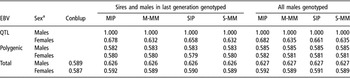
Table 5 shows the accuracies of QTL–EBV, polygenic EBV and total EBV for the scenarios where only sires and males in last generation were genotyped and all males were genotyped using different methods to predict gene content using regression on gene content in GA-BLUP, in comparison to conventional BLUP and GA-BLUP when all animals are genotyped. Differences between methods were rather small. Both MM methods (M-MM and S-MM) yielded almost identical results. MIP performed better than M-MM and S-MM, resulting in a higher accuracy of the QTL–EBV. SIP performed better than M-MM and S-MM, but worse than MIP. Although the QTL–EBV were estimated more accurately with MIP and SIP, the difference in accuracy of the total EBV was negligible.
Accuracies of quantitative trait loci (QTL)–estimated breeding values (EBV), polygenic EBV and total EBV for conventional BLUP (Conblup) and gene-assisted BLUP with regression on gene content when only sires and males in last generation are genotyped or when all males are genotyped with different methods to predict gene contents when the heritability is 0.30 and the QTL explains 15% of the genetic variance

MIP = multiple-marker iterative peeling; M-MM = multiple-marker mixed model; SIP = single-marker iterative peeling; S-MM = single-marker mixed model to predict gene content, i.e. the number of two alleles.
aMales are genotyped; females are ungenotyped.
Average of 100 replicates; standard errors are 0.000 for males for QTL–EBV, 0.004 for females for QTL–EBV, 0.003 for polygenic and total EBV for both sexes, all methods and both scenarios.
Estimation of allele substitution effect
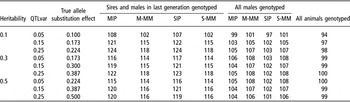
Table 6 shows the estimated allele substitution effect as a percentage of the true simulated allele substitution effect for different combinations of heritability and QTL variance using GA-BLUP with regression on gene content with different methods to predict gene contents. In most cases, the allele substitution effect was severely overestimated, especially when only sires and males in the last generation were genotyped. In the latter situation, the allele substitution effect absorbs part of the genetic trend in the polygenic term. The overestimation was slightly larger with MIP and SIP when sires and males in the last generation were genotyped than with M-MM and S-MM, but vice versa when all males were genotyped. The overestimation increased with higher proportion of genetic variance explained by the QTL. When all animals were genotyped, the allele substitution effects was close to the true value and slightly underestimated when the heritability was 0.10 and the QTL explained 5% of the genetic variance. Without selection, allele substitution effects were close to the true values also when only part of the animals was genotyped (results not shown). It can be concluded that inclusion of missing genotypes in data sets with selection can bias allele substitution effects, but the effect on accuracy of GA-BLUP is negligible.
The estimated allele substitution effect as a percentage of the true simulated allele substitution effect for gene-assisted BLUP when animals are all genotyped, when only sires and males in last generation are genotyped or when all males are genotyped with different methods to predict gene contents for different values of heritability and quantitative trait loci variance (QTLvar)

MIP = multiple-marker iterative peeling; M-MM = multiple-marker mixed model; SIP = single-marker iterative peeling; S-MM = single-marker mixed model to predict gene content, i.e. the number of two alleles.
Average of 100 replicates; standard errors of estimated allele substitution effects are 0.002–0.009.
Discussion
Methods and results
In this study, different methods were compared in their ability to deal with missing genotypes in gene-assisted breeding value estimation, when the gene is known. Regression on predicted gene content was compared to using an inverse IBD matrix based on linkage analysis information (IBD–LA) in the MM equations. In addition, MIP and MM predictions were compared to predict gene content for genotyped and ungenotyped animals. As expected, regression on gene content performed better than the IBD–LA method, resulting in slightly higher accuracies of the total EBV. MIP performed better than SIP and the MM methods to predict gene content, but differences in accuracy of total EBV were rather small. Gengler et al. (Reference Gengler, Mayeres and Szydlowski2007) reported also very similar correlations between true and predicted gene contents using either the S-MM or SIP. Allele substitution effects were overestimated in agreement with Gengler et al. (Reference Gengler, Abras, Verkenne, Vanderick, Szydlowski and Renaville2008), but in disagreement with Baruch and Weller (Reference Baruch and Weller2009), who found that allele substitution effects were underestimated. Clearly, the overestimation is partly due to genotyping only a selected group of sires in generations 1 to 4 (see Table 6), whereas Baruch and Weller (Reference Baruch and Weller2009) genotyped all bulls in each generation. Gengler et al. (Reference Gengler, Mayeres and Szydlowski2007) reported significant improvement of prediction of gene contents over the method of Israel and Weller (Reference Israel and Weller1998), which was also used in Baruch and Weller (Reference Baruch and Weller2009). The improvement in prediction of gene content may explain also the difference in results between Baruch and Weller (Reference Baruch and Weller2009) on one side and Gengler et al. (Reference Gengler, Mayeres and Szydlowski2007) and this study on the other side.
The IBD–LA method performed worse than regression on gene contents. The assumption of the IBD method is that the locus has an infinite number of alleles, which is clearly violated in the case of gene-assisted breeding value estimation with a QTL with two alleles. As a consequence, more effects need to be estimated, resulting in lower accuracy of the estimated haplotype effects and the total EBV (Villanueva et al., Reference Villanueva, Pong-Wong and Woolliams2002). Furthermore, in this study the IBD matrix was constructed using only linkage analysis information. Combining linkage disequilibrium and linkage analysis information as in LD/LA analysis is expected to improve the accuracy of the QTL–EBV and the total EBV. Meuwissen et al. (Reference Meuwissen, Karlsen, Lien, Olsaker and Goddard2002) showed that combined LD/LA analysis narrowed the likelihood peak around the putative QTL locus. In terms of breeding value estimation, LD information would increase the connectedness between the haplotypes increasing accuracy of the estimates. In addition to the results, we used LD/LA when all animals were genotyped and the accuracy of the QTL–EBV was 0.93 and the accuracy of the total EBV was only 0.004 lower than the accuracy of the total EBV with regression on gene content (based on 20 replicates with 5000 animals to limit computing time). This shows that inclusion of LD information in construction of the inverse IBD matrix increases accuracy, however, at the cost of extra computing time. Furthermore, inclusion of linkage disequilibrium information in the presence of missing genotypes of base animals is an unsolved problem.
Using information of flanking markers increased the accuracy of the QTL–EBV when using MIP. The multiple-marker extension of the MM method did, however, perform similar as the S-MM. MIP uses mainly linkage analysis information within families. Information of flanking markers makes it easier to determine paternal and maternal haplotypes. With the M-MM method, only LD information across families is used, which was low as indicated by r 2 ≈ 0.05 due to the relatively low marker density. Therefore, information of flanking markers increased the accuracy of QTL–EBV with MIP, but it did not increase accuracy of QTL–EBV with the M-MM method. The M-MM method might be useful to predict gene contents when certain animals are not genotyped on some loci, but have genotypes on other flanking loci and when marker densities are much higher resulting in higher correlations between markers. The M-MM method and the MIP method might be useful to predict gene contents of SNP markers in genomic selection in situations where animals have missing genotypes for some markers due to genotyping problems or differences in SNP arrays. The mixed model method is not only computationally advantageous, e.g. with 60 K SNP chips, but can also easily deal with genetic groups in the base population (Gengler et al., Reference Gengler, Mayeres and Szydlowski2007) and can be used to predict accurately allele frequencies in the base generation (VanRaden, Reference VanRaden2008).
Implications for breeding
This study shows that even ungenotyped animals benefit from gene-assisted breeding value estimation, although the increase is only substantial when the heritability of the trait is low and when the QTL explains a large proportion of the genetic variance. However, genotyping these animals would further increase the accuracy. Using information of flanking markers increases the accuracy of the total EBV only marginally at the marker density considered in this study. Therefore, if budgets for genotyping are limited, it is better to genotype as many animals for the gene as possible instead of genotyping fewer animals for the gene and some flanking markers. On the contrary, it is not expected that selection response increase substantially when increasing the proportion of genotyped animals to 100%. Ansari-Mahyari et al. (Reference Ansari-Mahyari, Sorensen, Lund, Thomsen and Berg2008) found that genotyping respectively 20% and 50% of the selection candidates would yield 89% and 95% of the maximum response. For gene-assisted as well as genomic selection, it is worth to have at least 1000 animals genotyped to get accurate estimates of SNP effects (Goddard, Reference Goddard2009).
In this study, it was found that the advantage of gene-assisted breeding value estimation is greater when the heritability is low and when the QTL is explaining a large proportion of the genetic variance. This is in accordance with other studies (Lande and Thompson, Reference Lande and Thompson1990; Meuwissen and Goddard, Reference Meuwissen and Goddard1996; see reviews in Weller, Reference Weller2001; Dekkers and Van der Werf, Reference Dekkers and Van der Werf2007; Weller, Reference Weller2007) showing that gene- and marker-assisted is most beneficial for traits with a low heritability. In addition to other studies, results here indicate that for traits with low heritability (e.g. disease and fertility traits) even animals that are not genotyped can benefit from GA-BLUP when inferring their gene content based on marker information of genotyped relatives. As a consequence, response to selection will be higher when these ungenotyped animals are selected on GA-BLUP–EBV than on conventional BLUP–EBV. It is expected that genomic selection for ungenotyped animals using predicted gene contents for all SNP would be beneficial especially for low heritable traits.
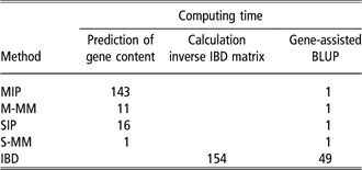
Methods applied in this study are applicable for national genetic evaluations, but some of them are rather time-consuming. Table 7 shows the computing time in seconds for the different parts of the calculations. Methods using multiple-marker iterative peeling (MIP and IBD) are both more time-consuming than methods using multiple-marker and single-marker mixed models. The IBD–LA method is using an enormous amount of time, because in addition to running MIP, the inverse IBD matrix needs to be constructed with the Fernando and Grossman (Reference Fernando and Grossman1989) rules. Furthermore, breeding value estimation with the IBD–LA method takes more time than when regressing on gene contents. This is because many more MM equations need to be solved. In addition, the current implementation of using inverse IBD matrices in MiX99 (core program described in Lidauer and Stranden (Reference Lidauer and Stranden1999)) may not be optimized in terms of computing time. Based on accuracy and computing time, the S-MM method as developed by Gengler et al. (Reference Gengler, Mayeres and Szydlowski2007 and Reference Gengler, Abras, Verkenne, Vanderick, Szydlowski and Renaville2008) is practically the best method to use for national genetic evaluation with inclusion of effects of genes combining phenotypic information of genotyped and ungenotyped animals.
Computing timeFootnote a in seconds (average of 20 replicates) for predicting gene content with multi-marker iterative peeling (MIP), multi-marker BLUP, single-marker iterative peeling and single-marker BLUP, for creating the inverse identity-by-descent relationship matrix using genotype probabilities from MIP and for gene-assisted BLUP in the situation where sires and males in the last generation are genotyped
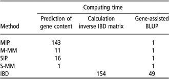
M-MM = multiple-marker mixed model; SIP = single-marker iterative peeling; S-MM = single-marker mixed model to predict gene content, i.e. the number of two alleles; IBD = identity-by-descent relationship method.
a On a dual-processor 64-bit PC with 2.40 GHz and 8 GB of RAM; programs were compiled for 32-bit.
Conclusion
This study shows that gene-assisted breeding value estimation increases accuracies of total EBV in comparison to conventional breeding value estimation. The increase in accuracy was much lower (0% to 5%) for animals that were not genotyped compared to genotyped animals (0% to 22%), but still substantial when the heritability was 0.1 and when the QTL explained at least 15% of the genetic variance. Regression on predicted gene content yields higher accuracies than using an IBD method based on linkage analysis information. Missing gene contents can be predicted most accurate using MIP, while the mixed model methodology is computationally much faster. For large livestock populations, gene-assisted breeding value estimation can be best performed by regression on gene contents, using mixed model methodology to predict missing genotypes. This technique would be, in principle, also feasible for genomic selection using dense SNP chips. It is expected that genomic selection for ungenotyped animals using predicted SNP gene contents might be beneficial especially for low heritable traits.
Acknowledgements
Egbert Knol, Dieuwke Roelofs-Prins, Marc Rutten, Chris Schrooten, Addie Vereijken are gratefully acknowledged for helpful discussions about this study. We are indebted to Martin Lidauer, Ismo Stranden, Kaarina Matilainen, Esa Mantysaari and Robin Thompson for discussions and implementation of using IBD matrices in MiX99.
The work was financially supported by CRV, Hendrix Genetics and IPG and has been co-financed by the European Commission, within the 6th Framework Programme, contract No. FOOD-CT-2006-016250 (SABRE). The text represents the authors’ views and does not necessarily represent a position of the Commission who will not be liable for the use made of such information.
Appendix 1 Use of LD information from SNP markers in MIP to estimate the phase of the founder animals
Our strategy was to include the LD information into the prior probabilities of the genotypes of the founder animals, i.e. the animals on the top of the pedigree whose parents are unknown. Without the use of LD information, the prior probability of their genotypes is Prior(X 1, X 2) = p(X 1) p(X 2), where X 1 (X 2) denotes the SNP allele at chromosome 1 (2) at locus X, i.e. X 1 = 0 (X 1 = 1) denotes that the ‘0’ (‘1’) allele is carried at this locus, and p(X 1) is the allele frequency of X 1. Which chromosome is called 1 or 2 is arbitrarily decided by the MIP algorithm, and is not relevant for the estimation of the phase. Thus, we attempt here to improve Prior(X 1,X 2) probabilities by including the LD information. For the estimation of marker phases of the descendants of the founder animals, the linkage analysis information is used by the MIP algorithm. However, if the estimation of the marker phases of the founder animals is improved by the inclusion of LD information, the estimates of the marker phases of the descendants will also improve.
The general approach taken is that we will attempt to predict Prob(X 1 = 1) by using the genotypes at surrounding markers at chromosome 1, and using multivariate regression to regress X 1 onto the genotypes of the surrounding markers. However, instead of using traditional multivariate regression, Partial Least Squares Regression (PLSR; Martens and Naess, Reference Martens and Naess1989) will be used, in order to avoid over-fitting of the data. In the following we will drop the subscript ‘1’ denoting the chromosome, for ease of notation. The described procedure will be applied to each of the chromosomes of all the founder animals and for all the loci. The prediction by multiple regression is:

where Z the vector of marker genotypes at the surrounding loci (all elements 0 or 1), pX is the frequency of the X = 1 allele, i.e. E(X) = pX; pZ is a vector of frequencies of each of the alleles at loci Z being allele 1. In case of traditional regression, b = CV−1, where C is a row vector of covariances between X and Z’, and V is the variance/covariance matrix of Z. For PLSR, we also need to estimate the matrices C and V, and this is described below.
First, we need to decide which are the surrounding markers of locus X, i.e. which loci are included in Z. As potential candidates, we consider 20 loci to the left of X (or fewer if the chromosome end is reached) and 20 loci to the right of X (or fewer if the chromosome ends). If for any locus Zi, the genotype of the founder chromosome cannot be established with reasonable certainty (>0.9 as estimated by the MIP algorithm), locus Zi is eliminated from the set of surrounding markers. Second, the variance of the remaining loci Zi are estimated, next to the covariances of Zi with all other surrounding loci Zj and X in order to obtain all the elements of C and V. For these (co)variance estimations, all chromosomes are used for which the required genotypes are estimated with reasonable certainty (>0.9). If the latter results in that any of the (co)variance estimates involving locus Zi is based on less than 50 chromosomes, the locus Zi is removed from the set of surrounding loci.
The above describes the estimation of the (co)variance matrices C and V, which are needed for the PLSR regression. For a detailed description of PLSR, see Martens and Naess (Reference Martens and Naess1989). Briefly, it attempts to reduce the dimensionality of the regression by setting up k latent variables, which are linear combinations of the variates Z. The latent variables are constructed such that they best predict X. We used here k = 2, i.e. the two best latent variables were used to predict X. Some preliminary testing indicated that predictions did not improve markedly by using k > 2. If the estimates of P(X = 1) were higher than 0.98 (or lower than 0.02), P(X = 1) was set to 0.98 (0.02) in order to avoid that the prior information completely determines the genotype.
Next, the Prior(X 1, X 2), including LD information, was calculated as:

The complete algorithm consisted of the following steps:
Step 1: Run the MIP algorithm without LD information until convergence;
Step 2: Include LD information as described above into the prior probabilities;
Step 3: Use one iteration of the MIP algorithm;
Step 4: If the sum of square of the changes in genotype probabilities divided by the total sum of square of the genotype probabilities is less than 10−4: finish; otherwise return to step 2.